
Estimation of Final Product Concentration in Metalic Ores Using Convolutional Neural Networks
by
 , , , and
Jakub Progorowicz
1 ,
,
Artur Skoczylas
2,
Sergii Anufriiev
2,*,
Marek Dudzik
1,3 and
Paweł Stefaniak
2 1
Comex Polska Ltd., Kamienskiego 51, 30-644 Krakow, Poland
2
KGHM Cuprum—Research and Development Centre Ltd., Gen. W. Sikorskiego Street 2-8, 53-659 Wroclaw, Poland
3
Cracow University of Technology, Faculty of Electrical and Computer Engineering, Warszawska 24, 31-155 Krakow, Poland
*
Author to whom correspondence should be addressed.
Minerals 2022, 12(12), 1480; https://doi.org/10.3390/min12121480
Submission received: 10 October 2022
/
Revised: 9 November 2022
/
Accepted: 14 November 2022
/
Published: 22 November 2022
(This article belongs to the Special Issue Innovative Solutions for Measurements, Modelling and Control in Mineral Processing)
Abstract
:Although artificial neural networks are widely used in various fields, including mining and mineral processing, they can be problematic for appropriately choosing the model architecture and parameters. In this article, we describe a procedure for the optimization of the structure of a convolutional neural network model developed for the purposes of metallic ore pre-concentration. The developed model takes as an input two-band X-ray scans of ore grains, and for each scan two values corresponding to concentrations of zinc and lead are returned by the model. The whole process of sample preparation and data augmentation, optimization of the model hyperparameters and training of selected models is described. The ten best models were trained ten times each in order to select the best possible one. We were able to achieve a Pearson coefficient of R = 0.944 for the best model. The detailed results of this model are shown, and finally, its applicability and limitations in real-world scenarios are discussed.
1. Introduction
Grain size distribution and chemical composition are the basic parameters determining the effectiveness of mineral processing. Knowing them makes it possible to properly select the operating parameters and evaluate the efficiency of the ore enrichment processes. Traditional recognition methods, such as sieve analysis or laboratory tests, are not feasible in real-time and are very costly and time-consuming. They are carried on the macro- and micro-scale [1,2]. Additionally, there are a number of factors that can make the sample unrepresentative and not yield consistent results. In practice, vision-based methods for the analysis of the material stream are being increasingly used [3,4]. There are works in the literature where vision methods were used to assess the quality of the applied chemicals [5] or to assess the color of juice powders [6]. One of the most common transportation means used for a large amount of granular material is the conveyor belt, in which only the surface layer is visible to the vision system. The basic problem of this system concerns the inherent overlap and segregation of particles, or the location of small fragments under a larger one [1]. The reduction in the three-dimensional shape of the surface of the material flow to the form of a two-dimensional image prevents the precise reproduction of the volume and weight of both individual grains and the entire material flow. On the other hand, the use of fusion from various sources allows to extract unique features, thanks to which it is possible to estimate the physical and chemical properties of individual minerals.
1.1. Grain Size Distribution—State of the Art
Most of the vision methods used in mining to analyze the output transported through the conveyor belt relate to monitoring and controlling particle size distribution. This solution is essential to improve energy consumption and metallurgical efficiency [7,8,9,10]. Overall, machine vision seems to be the best approach at the moment as it is robust, cost-effective, non-invasive and online. There are many works related to online optical sizing systems for coarse rocks and iron pellets in the literature. The first methods based on machine vision and image processing technology appeared at the turn of the 1980s and 1990s [11,12]. Early methods relied on detecting the contours of the ore, converting two-dimensional images of ore into three-dimensional characteristics, such as particle size distribution and incoming ore volume. In the article in [12], the authors described the hardware and software along with the whole mechanism of converting video data to volumetric (sieve) data, including solutions to common problems related to particles overlapping or extraction of particles from a dirty conveyor belt background, etc. The rapid development of new technologies after 2000 started advances in the area of estimating grain size distribution. For example, in [13,14], the authors extracted information about RGB color and the visual texture of particles. They used the radial basis neural network to control the ore classification and sorting process. In the article in [15], the authors presented a method developed for the crushing circuit of a copper concentrator based on image and neural network processing. The methods of segmentation of visual images and extraction of size features were presented, and their potential was assessed on the basis of a test sample developed in the sieve analysis. In [16], the authors present an approach to crushed ore analysis using data on belt weight and a 3D laser scanner. On the other hand, the authors of [17] used a number of non-invasive tomographic sensors encased above the moving conveyor belt to estimate the particle size distribution. In [18], the authors developed a method for the detection of oversized ore pieces based on computer vision and sound processing for the purpose of validating vibration signals in the diagnostics of mining screen. Another interesting method based on deep learning and image technology is introduced in [19]. The developed model enables the detection of empty belt images, segmenting the coarse material images as well as mixed material images. The authors achieved an accuracy of 94.4%. In subsequent works, multi-layer perceptron networks (MLPN) and statistical networks (machine learning) were used to identify granular material and its impurities [20]. The increased popularity of inspection robotics in the mining sector contributed significantly to the further development of the optical sizing system for ore classification on the belt [21,22].
1.2. Chemical Composition
The first works on the use of machine vision to recognize minerals in rock began to appear in the 1990s. They were based on methods such as color vector angle or two-dimensional texture analysis [23,24]. Currently, predicting the chemical composition of ore streams based on the analysis of visual data most often assumes the analysis of the response in the light spectrum from the X-ray to the IR range. The physical phenomenon mainly used here is fluorescence, which is the emission of electromagnetic radiation after excitation of the medium (e.g., by means of ultraviolet light). The excitation of the material is monitored by means of specialized sensors designed for this purpose, e.g., vision cameras and a wide spectrum of recordings. These sensors contain data in various formats, such as a 2D image in the form of a PNG file, a spectrum in the wavelength domain or a 3D image. As a result of excitation, the material produces electromagnetic radiation at a different wavelength from the light, causing excitation. This makes possible to use filters to isolate the response of the rock material. From this response (regardless of the data format), after appropriate processing, parameters are obtained, which are the input data to the classifier. The methods found in the literature are mainly used in geology and are based on multi-source and multi-type mineral datasets processed with the use of machine learning techniques [25,26,27]. However, more and more often artificial neural networks are being used for this purpose. In the article in [28], the authors used a neuro-adaptive learning algorithm for real-time classification of iron ore. A comprehensive recognition model for 12 types of rock minerals has been described in the article in [29]. The proposed approach is based on deep learning and transfer learning algorithms. A solution based on neural networks for sorting and classifying enriched iron, manganese and alumina particles was presented in [13]. In publication [30], the authors presented a vision system for sorting crushed aggregates. The wavelet analysis, the Canny edge detection method and the PCA algorithm were used to extract the textural features. A similar solution for nickel ore can be found in the article in [31].
1.3. Aim of the Article
The article was written as part of the development of innovative pre-concentration technology on the example of a selected raw material using a Comex Poland sorting machine equipped with a hybrid analysis system and artificial intelligence algorithms. A novel analysis system was developed with a decision-making process based on neural networks fed with data from multi-parameter X-ray and optical analysis in the ultraviolet and infrared spectra. As a result, a demonstrator of a sorting line for the pre-concentration of ingredients of useful raw materials was obtained. The article presents an example of a neural network model for the automatic classification of sorted grains based on the prediction of the percentage of useful components in the ore stream. For the purpose of this article, only X-ray images were used. The integration of other sources of images into product concentration estimation algorithms is planned in further stages of the project.
1.4. General Model Description
Artificial Neural Networks (ANN) are a group of machine learning algorithms inspired by the structure of the human brain. ANNs allow for solving a number of analytical tasks such as regression [32,33], classification, grouping and many others. The classic neural network model (perceptron) consists of three types of layers: (1) input layer—the number of neurons is equal to the number of input variables (e.g., the number of pixels in the image), (2) the output layer—the number of neurons is equal to the number of classes and (3) hidden layers—increase the possibilities of generalization (the more hidden layers, the more complex dependencies the network is able to detect). The classification of visual images is carried out using convolutional neural networks, the main idea of which is to filter the images before they reach the remaining layers of the neural network. It is created through the convolutional layers in which each neuron has one filter assigned to it. All filters are user-defined and randomly initialized. The transformation of the signal when it reaches the convolution layer consists in the operation of combining (convolution) the filter with the image. Each filter detects one pattern, e.g., geometric filters detect straight lines, squares or circles. As the network grows, the pattern detected by filters becomes more and more complex.
In this article, such an approach is tested in application to mineral processing, particularly to initial filtration of the incoming ore. Compared with other similar articles dedicated to ANN applications, we not only present here the proposed structure but also describe our approach to structure optimization.
2. Materials and Methods
2.1. Data Description
This article uses two types of data: X-ray scans obtained using Dual-Energy technology (RTX DE) and concentrations of zinc and lead obtained with X-ray fluorescence method (XRF). Input data to the network were prepared on a real facility using the infrastructure of COMEX Poland Sp.z o.o.. The ore comes from the Lovisa mine in Sweden. The Python programming language was used for all calculations. The Tensorflow library was used for model learning, while the Thalos library for model structure optimization.
The sample includes 2 size fractions (approximately 20–40 mm and 40–70 mm), 31 pieces of ore each. For each ore piece, low-energy and high-energy scans are made. For smaller fractions, the resolution of images is 64 × 64 pixels, while for larger fractions it is 76 × 76 pixels. In order to prepare a single model for both fractions, the smaller images are padded with minimum value (6-pixel padding from each side). In order to increase the number of samples, and thus improve model performance, several scans with different orientations of the grain were performed. For smaller fraction, 5 scans were made, while for the larger one 7 scans were performed.
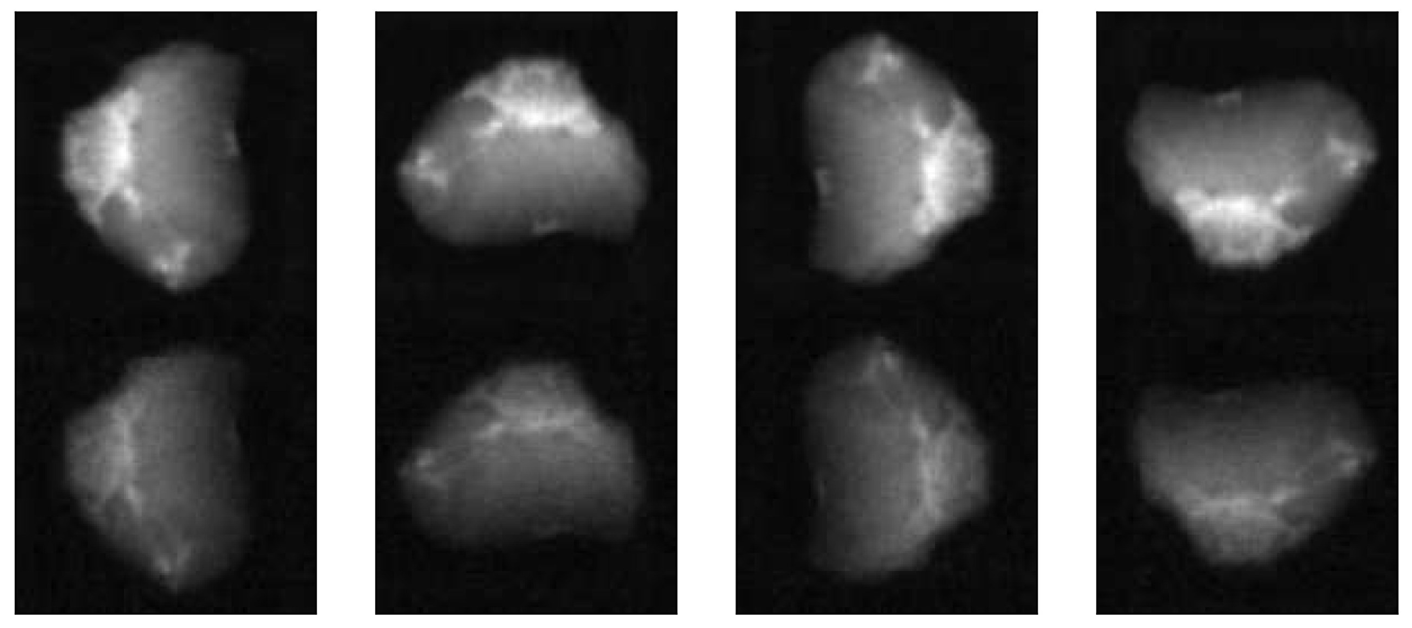
In the next step, the low- and high-energy scans were stacked vertically. As a result, 377 images with a resolution of 76 × 152 pixels were obtained. Finally, during the model training phase, the data were augmented with images rotated over 90, 180 and 270 degrees. An example of original images and rotated images is shown in the Figure 1.
For each grain, the concentrations of zinc and lead were defined using X-ray fluorescence method. The concentrations defined this way were then used as labels during the training of a neuron-network-based model for estimation of the concentration based on the scans described above.
2.2. Model Description
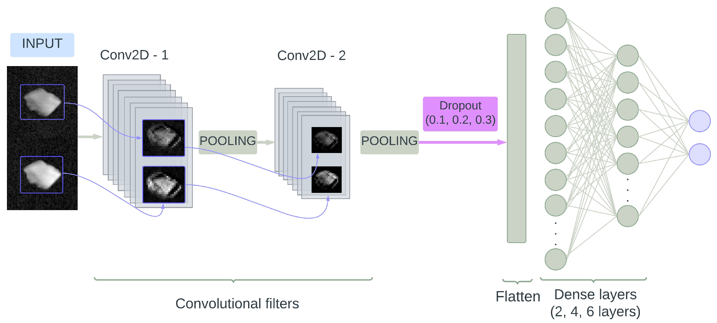
Convolutional neural networks have shown themselves as a perfect solution for image analysis, thus such a model was chosen for this problem. The overall architecture of the tested models is shown in Figure 2.
The model consists of two main blocks: convolutional and dense [32,33,34]. The convolutional block includes convolutional layers and pooling layers. After the convolutional block, a dropout layer is included in order to eliminate the overfitting effect. Then, a flatten layer is applied. Finally, a dense block consisting of consecutive dense layers is added to the model. An output layer is another dense layer with 2 neurons: the first one represents the zinc concentration, while the second one represents lead concentration. The exact number of particular layers, as well as model hypermarameters, such as activation functions, learning rate, optimizers, etc., were defined during the optimization procedure, which is described in the next section.
2.3. Structure Optimization Procedure
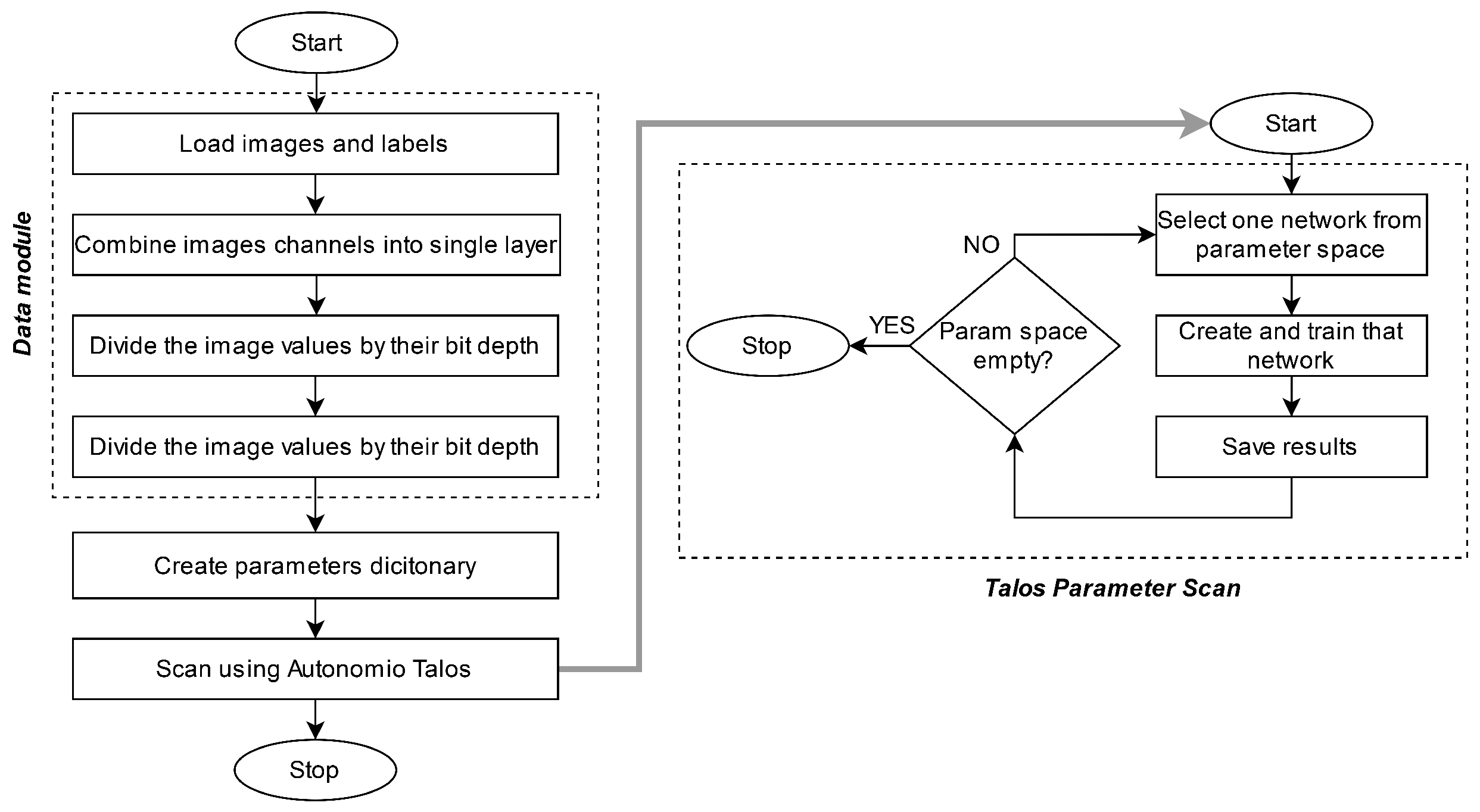
Although neural networks in many cases give very promising results, choosing an appropriate structure and defining optimal hyperparameters of the model is always a challenge. In this article, the Talos library [35] was used in order to define the optimal structure. The algorithmic scheme of the optimization procedure is shown in Figure 3. The models were trained for 51,840 sets of network structures and training parameters listed in Table 1.
The data were divided into training, validation and test sets in the proportion 3:1:1. In addition to the parameters shown in Table 1, the following static values were used: learning rate at 0.001. The value of the assumed learning rate resulted from the optimization of the hyperparameters procedure at an earlier stage of the research. Finally, each model included 2 convolutional layers, the second one had two times less filters then the first one.
In the first step, every model was trained once. The detailed procedure of this step is presented in Figure 3. Based on the values of validation of the mean absolute error, the ten best structures were selected and then assessed from robustness, underfitting and overfitting perspectives.
3. Results
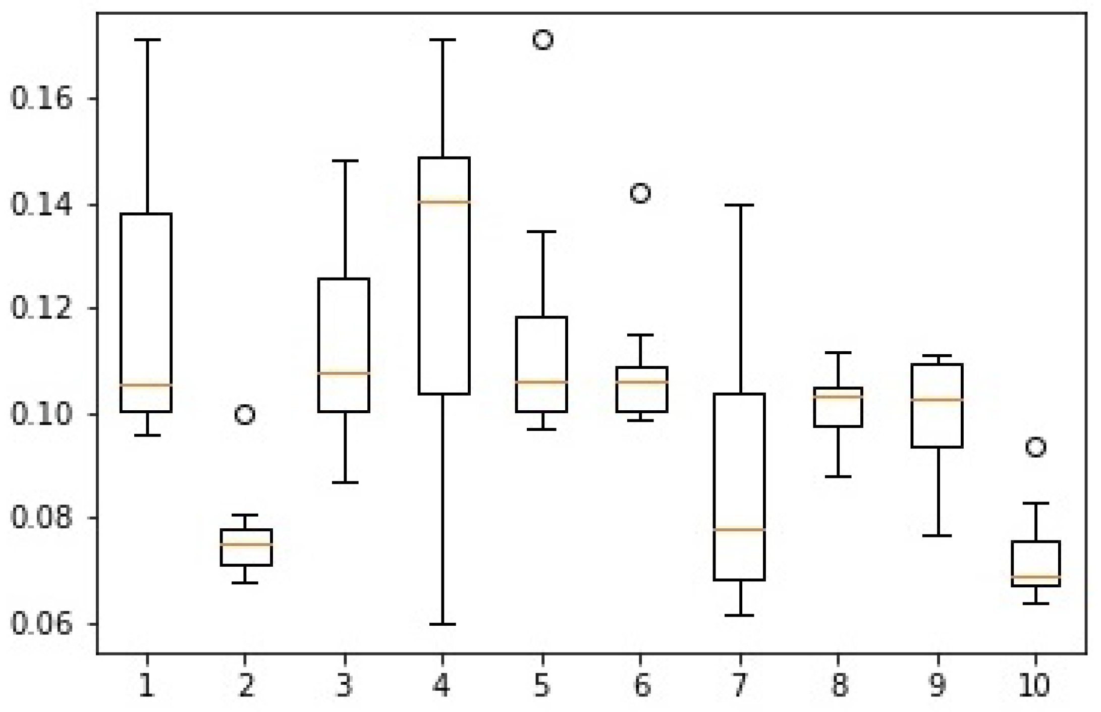
Figure 4 shows a box plot obtained from the network structure optimization procedure. The results presented in the figure are mean absolute values calculated for the best ten structures. These structures were considered as potentially optimal. The details of these ten models are presented in the Table 2. The identification of the optimal structure was performed according to the procedure described in detail in [34]. The usefulness of this method in practical applications is described and proven in [32,33,34]. The method is also in use in the Comex Poland Sp. z.o.o. company.
As can be seen in Figure 4, the structures with indices 1, 3, 4, 5, 7 and 9 show a strong influence of randomly initiated initial conditions of the learning process, which proves that despite the implementation of dropout layers inside the structures, there is a high probability of overfitting phenomena occurrence. Structures 6 and 8 show a significantly lower variability of MAE than in the case of all the structures mentioned above. However, on the other hand, the average value of MAE for them is much higher than the corresponding values for structures 2 and 10. Thus, these two structures (2 and 10) are taken into account as potentially optimal.
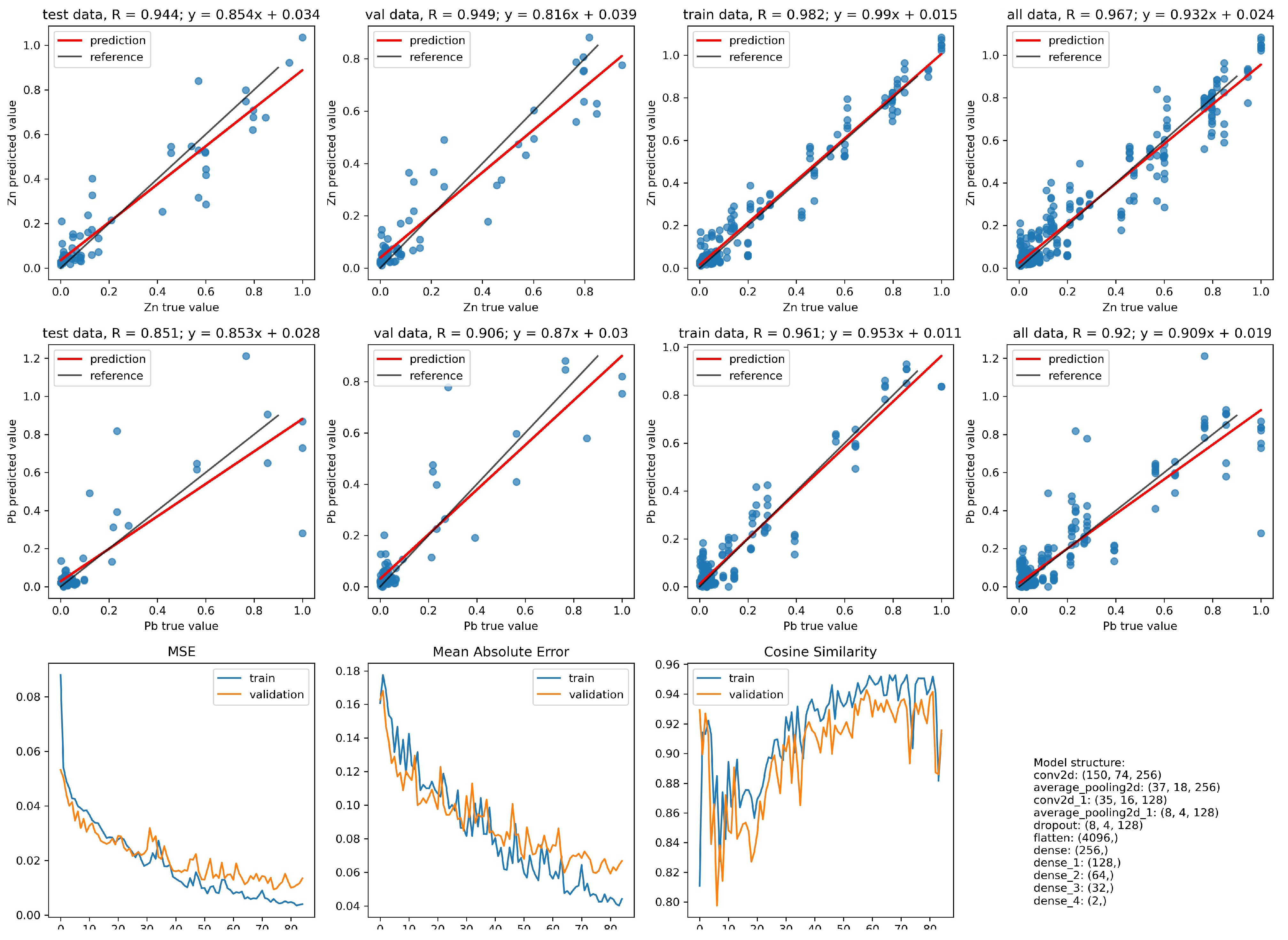
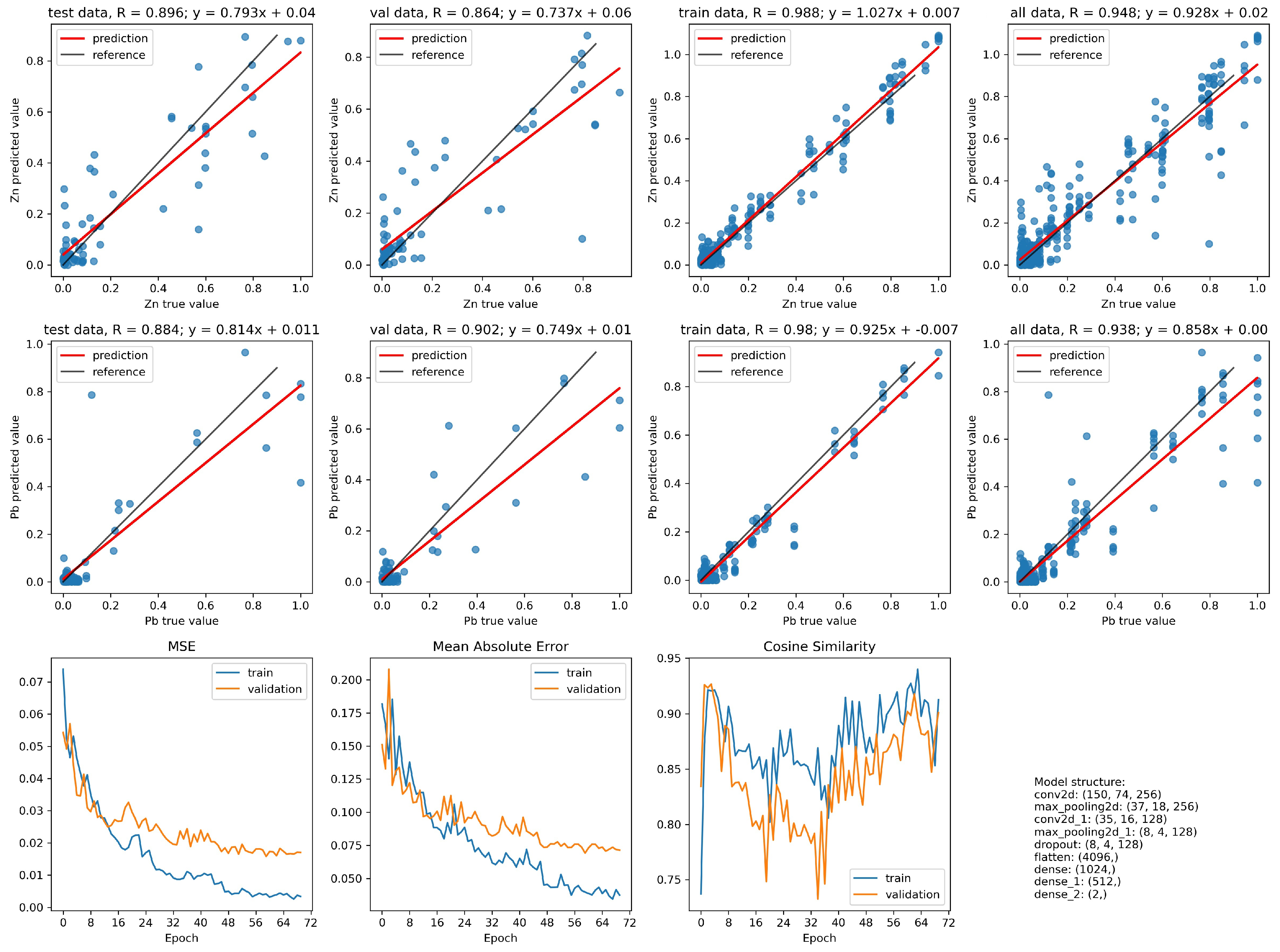
Figure 5 and Figure 6 present the calculation results of the network regression coefficients and their qualitative indicators resulting from the conducted learning process. The results shown in Figure 5 refer to the best network with index 10. In turn, those shown in Figure 6 refer to the best network with index 2.
At first glance, the results shown in Figure 5 and Figure 6 indicate that both of the taught networks are usable. Based on the results for the network test stage, it can be seen that in the case of zinc content in the rock, the neural network with index 10 obtains much better convergence than the network with index 2. In the case of the network with index 10, the Pearson regression coefficient obtained value is 0.944, while for the network with index 2, the value of this coefficient is 0.896, which is over 5% less. This means also that the structure of the neural network with the index 10 more effectively links the value of the zinc concentration from the chemical analysis with the features resulting from the X-ray scans of the grains. On the other hand, the network with index 2 has slightly higher values of Pearson coefficient for lead, but this difference is lower than in the case of zinc.
When analyzing the structures of the network with indices 2 and 10 (the description of which is in the lower right part of Figure 5 and Figure 6), it can be noticed that the complexity of the convolutional layers is the same. That is, both the first and second conv2d layers have the same configuration. The same goes for the dropout layer. However, the only difference in the design of the convolution filter concerns the use of the condense feature extraction tool [36]. In the case of the network with index 10, the averagepooling2D technique was used, while for network with index 2, the technique of maxpooling2D was used. This means that in the proposed network model (Figure 2), the configuration of conv2d and dropout layers is optimal.
It should be noted that depending on the condense feature extraction techniques used in the networks with indexes 2 and 10, the complexity of the dense layer parts differs. In the analyzed case, the situation in the dense layer is natural, and it manifests smaller dense layers in the network with averagepooling2D layer compared with the network with maxpooling2D layer. However, the averagepooling2D case needs a deeper dense layers network.
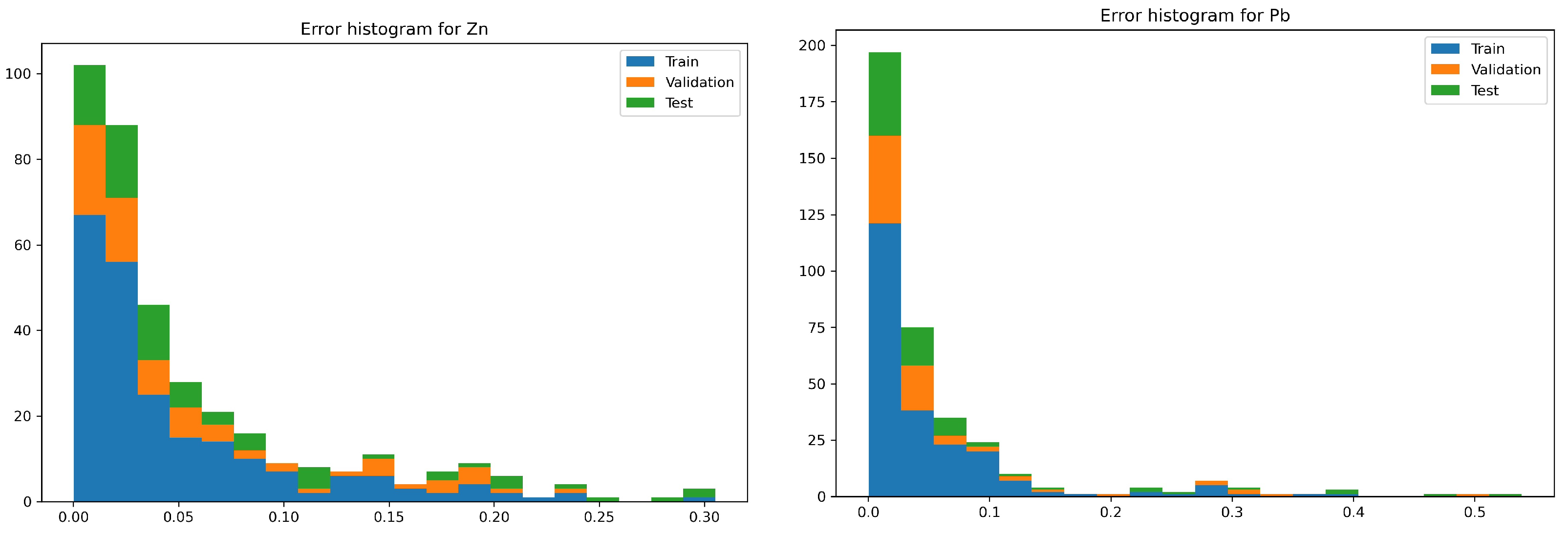
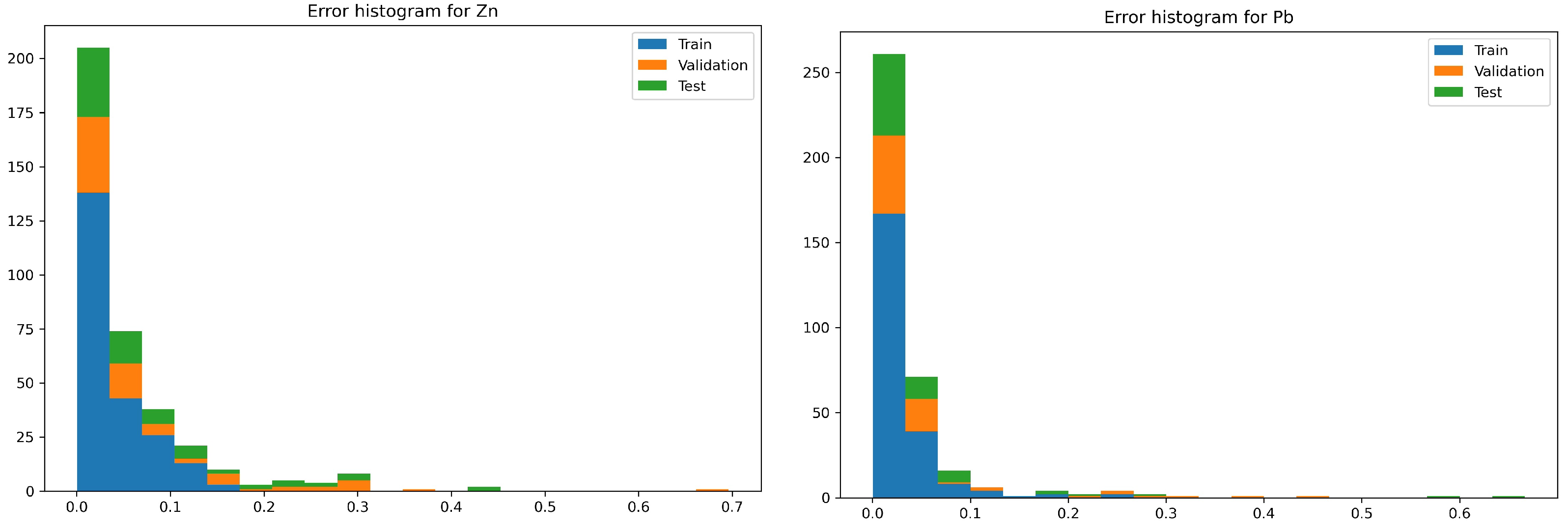
Additional assessment of the network convergence was performed on the basis of errors made by the network [32]. This assessment was made thanks to the error histograms, which are presented in Figure 7 and Figure 8. These histograms were drawn separately to identify the zinc and lead content in the ore grain using its scan. Figure 7 shows error histograms for the network with index 10, while Figure 8 relates to the network with index 2.
On the error histogram for zinc content in the grain plotted for the network with the index 10 (Figure 7), it can be seen that the maximum error made by the network is 0.3. However, such high error occurs for a marginal number of cases on both training and testing stages. The analyzed histogram shows that in most cases (samples > 25) this error fits in the range of values between 0 and 0.05.
In turn, the error histogram for the lead content in the grain for the network with the index 10 shows that the maximum error made by the network is 0.52. It occurs only for the network testing stage and is also of a marginal nature. It is noteworthy that in most cases (samples > 25) the error occurs in the range between 0 and 0.06.
On the error histogram for zinc content in the grain plotted for the network with the index 2 (Figure 8), it can be seen that the maximum error made by the network is 0.7. This error occurs for a marginal number of cases on the validation stage. The analyzed histogram shows that in most cases (samples > 25) this error occurs in the range of values between 0 and 0.1.
The error histogram for the lead content in the grain for the network with the index 2 (Figure 8) presents that the maximum error made by the network is 0.64. As for the network with index 10, it occurs only for the network testing stage and is also of a marginal nature. Ultimately, it can be said that the network with index 2 in most cases (samples > 25) has errors in the range between 0 and 0.06.
4. Discussion
In order to chose the best structure for the described problem, the results presented in the previous section were analyzed thoroughly. The analysis of regression results for networks with indexes 2 and 10 showed that:
- In the case of identifying the value of the zinc content in the grain, the network with the index 10 is characterized by a better convergence to the results with the values obtained from the chemical analysis. The improvement in convergence in this case is at the level of 5%.
- When identifying the value of the lead content in the grain, the network with the index 2 has a slightly better convergence than the network with the index 10. However, this disproportion is not as significant as it was in the case of zinc content for the network with the index 10.
The regression analysis showed that the network structure with the index 10 has optimal settings for the data assigned to the learning process. Nevertheless, it was necessary to evaluate the value of network errors using error histograms in order to make a final decision.
The analysis of error histograms for networks with indexes 2 and 10 showed that:
- In case of identifying the value of the zinc content in the grain:
- The network with the index 10 is characterized by more than a twice lower maximum error. The number of occurrences of this error for both networks is so marginal that the situation is negligible.
- The network with the index 10 in relation to the network with the index 2, for most of the analyzed cases, has twice the convergence of the output values with respect to the targets.
- In the case of identifying the value of the lead content in the grain:
- The network with index 10 is characterized by a smaller maximum error compared with the network with index 2. The occurrence of this error for both networks takes place at a level so marginal that it is negligible.
- Network errors with indexes 2 and 10 for most of the analyzed cases are in the range between 0 and 0.06.
Based on the above assessment, it is concluded that the network with the index 10 is optimal for the data assigned to the learning process in the scope of the structure shown in Figure 2.
Although in the past ANNs have been used in several use cases, the direct comparison of proposed models with them is tricky for two reasons. The first one is related to the large number of parameters for such models, which have to be fine-tuned for every use case. Thus, neither direct application of the previously developed models to our data nor the vice-versa approach will give satisfactory results. That is why we believe that the described network architecture optimization procedure is particularly important and potentially valuable for future applications of ANNs in problems related to mining and mineral processing.
The second reason is related to the selected machine learning approach. In most cases, the classification framework is chosen, which means that every data point has a class label assigned to it, and the model tries to predict this label. Usually, there are a very limited number of these classes, while the model performance is assessed based on accuracy metrics, i.e., the percentage of data points that were classified correctly. In this article, we solve the problem from a regression perspective, which means that the model is trying to predict the exact values of zinc and lead concentrations in each ore grain. Such an approach gives more flexibility in further application of the model because an arbitrary threshold can be used on the further steps of the process to separate waste and product fractions.
Although the values of accuracy and Pearson coefficient cannot be compared directly, they both fit into the [0, 1] interval; thus, we estimate how each model performs compared with a perfect scenario. In the most recent work, where a similar problem was considered [37], a Deep Neural Network model obtained an accuracy of 0.97 for the ore classification problem. This is comparable to the 0.944 Pearson coefficient obtained by our network in the case of zinc concentration prediction. Such difference can be explained by the difference in the input data for the model. In the above-mentioned article, the electrical resistivity, chargeability and magnetic susceptibility of each sample were measured in laboratory conditions and then used as features for model training. Such a small number of features makes it easier to train the model on a limited number of samples. We use X-ray scans, which result in a much higher number of features for model learning. At the same time, they are easier to collect, thus the ore classification can be performed in real time for material moving on the belt conveyor.
Several limitation should be taken into account. In this article, only relatively shallow network architectures were taken into consideration. It was dictated by two reasons: the first one is the model execution time limitations, and the second one is the limited amount of data available. Due to the nature of the industrial process, where the technology is going to be applied, the concentration estimation should be performed for multiple grains in fractions of a second, thus the complexity of the model structure should be adjusted to available computational capacity. At the same time, in order to train more complex models, a larger volume of input data might be needed to avoid model overtraining. If these two issues can be overcome in particular applications, more complex structures can be tested, which may further improve the results.
Despite these limitations, it was possible to obtain high correlation between regular X-ray scans and the results of XRF spectroscopy, which may be useful in industrial applications. In the future, it is planned to conduct similar investigations for other image acquisition technologies (infrared and visible light images and multi-energy X-ray scans) and study the possibilities to combine models developed for those sources together.
5. Conclusions
Ultimately, this publication presents both the complete process of the structure optimization and the assessment of selected network architectures, leading to the identification of the optimal network structure. The authors of the study did not find similar research in literature; therefore, they treat the presented results and conclusions as something that may direct other researchers to achieve better results in this field of study. The choice of the network structure optimization method turned out to be very beneficial in the studied case. Deeper analysis of the ten best structures chosen based on a single iteration of learning allowed to filter out 8 of 10 structures. The eight eliminated structures were either unstable or had a significantly higher mean absolute error. This means that choosing an optimal structure based only on a single run of training is not reliable enough for industrial applications. Importantly, the two best structures had the same complexity of convolutional filter, and the large differences between them resulted from the use of a different feature extraction technique. The application of the network structure optimization method showed that out of the four network training methods, two were characterized by satisfactory performance. They were RMSprop and Adam, which are the only two that appear among the ten best structures. The achieved accuracy of the selected models is sufficient for their further implementation and testing in industrial environment, which will be carried out in the later stages of the project.
Author Contributions
Conceptualization, J.P. and M.D.; methodology, M.D. and S.A.; software, A.S. and S.A.; validation, M.D. and P.S.; formal analysis, A.S.; investigation, M.D., S.A. and A.S.; resources, J.P.; data curation, J.P. and M.D.; writing—original draft preparation, M.D., S.A. and P.S.; writing—review and editing, J.P.; visualization, S.A. and A.S.; supervision, J.P. and P.S.; project administration, J.P; funding acquisition, J.P. All authors have read and agreed to the published version of the manuscript.
Funding
This research was funded by The National Centre for Research and Development grant number POIR.01.01.01-00-0884/20-00.
Data Availability Statement
Data used in the article will be shared with interested persons after signing of an NDA agreement with Comex Polska Ltd., Kamienskiego 51, 30-644 Krakow, Poland.
Conflicts of Interest
The authors declare no conflict of interest. The funders had no role in the design of the study; in the collection, analyses, or interpretation of data; in the writing of the manuscript, or in the decision to publish the results.
References
- Yeshi, K.; Wangdi, T.; Qusar, N.; Nettles, J.; Craig, S.R.; Schrempf, M.; Wangchuk, P. Geopharmaceuticals of Himalayan Sowa Rigpa medicine: Ethnopharmacological uses, mineral diversity, chemical identification and current utilization in Bhutan. J. Ethnopharmacol. 2018, 223, 99–112. [Google Scholar] [CrossRef] [PubMed]
- Rustom, L.E.; Poellmann, M.J.; Johnson, A.J.W. Mineralization in micropores of calcium phosphate scaffolds. Acta Biomater. 2019, 83, 435–455. [Google Scholar] [CrossRef]
- Gierz, Ł.; Markowski, P.; Chmielewski, P. Validation of an image-analysis-based method of measurement of the overall dimensions of seeds. J. Phys. Conf. Ser. 2021, 1736, 012007. [Google Scholar] [CrossRef]
- Gierz, Ł. The method and a stand for measuring aerodynamic forces in every plane on the basis of an image analysis. Proc. SPIE—Int. Soc. Opt. Eng. 2019, 11179, 111793F. [Google Scholar] [CrossRef]
- Gierz, Ł.; Gierz, S.; Koszela, K.; Fojud, A.; Boniecki, P.; Gawałek, J. Validation of a photogrammetric method for evaluating seed potato cover by a chemical agent. In Proceedings of the International Society for Optical Engineering, Shanghai, China, 11–14 May 2018; Volume 108064. [Google Scholar] [CrossRef]
- Przybył, K.; Gawałek, J.; Gierz, L.; Łukomski, M.; Zaborowicz, M.; Boniecki, P. Recognition of color changes in strawberry juice powders using self-organizing feature map. Proc. SPIE 2018, 10806, 1080621. [Google Scholar] [CrossRef]
- Yen, Y.K.; Lin, C.L.; Miller, J.D. Particle overlap and segregation problems in on-line coarse particle size measurement. Powder Technol. 1998, 98, 1–12. [Google Scholar] [CrossRef]
- Hahne, R.; Pålsson, B.I.; Samskog, P.O. Ore characterisation for—-And simulation of—-Primary autogenous grinding. Miner. Eng. 2003, 16, 13–19. [Google Scholar] [CrossRef]
- Tessier, J.; Duchesne, C.; Bartolacci, G. On-line multivariate image analysis of run-of-mine ore for control of grinding and mineral processing plants. In Proceedings of the International Conference on Mineral Processing, Modeling, Simulation and Control (MPMSC), Sudbury, ON, Canada, 6–7 June 2006; Volume 2006, pp. 175–189. [Google Scholar]
- Ko, Y.D.; Shang, H. A neural network-based soft sensor for particle size distribution using image analysis. Powder Technol. 2011, 212, 359–366. [Google Scholar] [CrossRef]
- Lange, T.B. Real-time measurement of the size distribution of rocks on a conveyor belt. IFAC Proc. Vol. 1988, 21, 25–34. [Google Scholar] [CrossRef]
- Lin, C.L.; Miller, J.D. The development of a PC, image-based, on-line particle-size analyzer. Min. Metall. Explor. 1993, 10, 29–35. [Google Scholar] [CrossRef]
- Singh, V.; Rao, S.M. Application of image processing and radial basis neural network techniques for ore sorting and ore classification. Miner. Eng. 2005, 18, 1412–1420. [Google Scholar] [CrossRef]
- Al-Sammarraie, M.A.J.; Gierz, Ł.; Przybył, K.; Koszela, K.; Szychta, M.; Brzykcy, J.; Baranowska, H.M. Predicting Fruit’s Sweetness Using Artificial Intelligence—Case Study: Orange. Appl. Sci. 2022, 12, 8233. [Google Scholar] [CrossRef]
- Hamzeloo, E.; Massinaei, M.; Mehrshad, N. Estimation of particle size distribution on an industrial conveyor belt using image analysis and neural networks. Powder Technol. 2014, 261, 185–190. [Google Scholar] [CrossRef]
- Thurley, M.J.; Andersson, T. An industrial 3D vision system for size measurement of iron ore green pellets using morphological image segmentation. Miner. Eng. 2008, 21, 405–415. [Google Scholar] [CrossRef] [Green Version]
- Williams, R.A.; Luke, S.P.; Ostrowski, K.L.; Bennett, M.A. Measurement of bulk particulates on belt conveyor using dielectric tomography. Chem. Eng. J. 2000, 77, 57–63. [Google Scholar] [CrossRef]
- Skoczylas, A.; Anufriiev, S.; Stefaniak, P. Oversized ore pieces detection method based on computer vision and sound processing for validation of vibrational signals in diagnostics of mining screen. In Proceedings of the International Multidisciplinary Scientific GeoConference: SGEM, Albena, Bulgaria, 18–24 August 2020; Volume 20, pp. 829–839. [Google Scholar]
- Ma, X.; Zhang, P.; Man, X.; Ou, L. A new belt ore image segmentation method based on the convolutional neural network and the image-processing technology. Minerals 2020, 10, 1115. [Google Scholar] [CrossRef]
- Gierz, Ł.; Przybył, K.; Koszela, K.; Duda, A.; Ostrowicz, W. The Use of Image Analysis to Detect Seed Contamination—A Case Study of Triticale. Sensors 2021, 21, 151. [Google Scholar] [CrossRef]
- Stachowiak, M.; Koperska, W.; Stefaniak, P.; Skoczylas, A.; Anufriiev, S. Procedures of detecting damage to a conveyor belt with use of an inspection legged robot for deep mine infrastructure. Minerals 2021, 11, 1040. [Google Scholar] [CrossRef]
- Dabek, P.; Szrek, J.; Zimroz, R.; Wodecki, J. An Automatic Procedure for Overheated Idler Detection in Belt Conveyors Using Fusion of Infrared and RGB Images Acquired during UGV Robot Inspection. Energies 2022, 15, 601. [Google Scholar] [CrossRef]
- Oestreich, J.M.; Tolley, W.K.; Rice, D.A. The development of a color sensor system to measure mineral compositions. Miner. Eng. 1995, 8, 31–39. [Google Scholar] [CrossRef]
- Petersen, K.R.P.; Aldrich, C.; Van Deventer, J.S.J. Analysis of ore particles based on textural pattern recognition. Miner. Eng. 1998, 11, 959–977. [Google Scholar] [CrossRef]
- Chen, J.; Chen, Y.; Wang, Q. Synthetic informational mineral resource prediction: Case study in Chifeng Region, Inner Mongolia, China. Earth Sci. Front. 2008, 15, 18–26. [Google Scholar] [CrossRef]
- Ślipek, B.; Młynarczuk, M. Application of pattern recognition methods to automatic identification of microscopic images of rocks registered under different polarization and lighting conditions. Geol. Geophys. Environ. 2013, 39, 373. [Google Scholar] [CrossRef] [Green Version]
- Shu, L.; McIsaac, K.; Osinski, G.R.; Francis, R. Unsupervised feature learning for autonomous rock image classification. Comput. Geosci. 2017, 106, 10–17. [Google Scholar] [CrossRef]
- Kitzig, M.C.; Kepic, A.; Grant, A. Near real-time classification of iron ore lithology by applying fuzzy inference systems to petrophysical downhole data. Minerals 2018, 8, 276. [Google Scholar] [CrossRef] [Green Version]
- Liu, C.; Li, M.; Zhang, Y.; Han, S.; Zhu, Y. An enhanced rock mineral recognition method integrating a deep learning model and clustering algorithm. Minerals 2019, 9, 516. [Google Scholar] [CrossRef] [Green Version]
- Murtagh, F.; Qiao, X.; Crookes, D.; Walsh, P.; Basheer, P.A.; Long, A.; Starck, J.L. A machine vision approach to the grading of crushed aggregate. Mach. Vis. Appl. 2005, 16, 229–235. [Google Scholar] [CrossRef]
- Tessier, J.; Duchesne, C.; Bartolacci, G. A machine vision approach to on-line estimation of run-of-mine ore composition on conveyor belts. Miner. Eng. 2007, 20, 1129–1144. [Google Scholar] [CrossRef]
- Dudzik, M.; Stręk, A.M. ANN Architecture Specifications for Modelling of Open-Cell Aluminum under Compression. Math. Probl. Eng. 2020, 2020, 2834317. [Google Scholar] [CrossRef]
- Dudzik, M.; Romanska-Zapala, A.; Bomberg, M. A Neural Network for Monitoring and Characterization of Buildings with Environmental Quality Management, Part 1: Verification under Steady State Conditions. Energies 2020, 13, 3469. [Google Scholar] [CrossRef]
- Dudzik, M. Towards Characterization of Indoor Environment in Smart Buildings: Modelling PMV Index Using Neural Network with One Hidden Layer. Sustainability 2020, 12, 6749. [Google Scholar] [CrossRef]
- Talos Library. Available online: https://pypi.org/project/talos/ (accessed on 30 May 2022).
- Maximum Pooling. Available online: https://www.kaggle.com/code/ryanholbrook/maximum-pooling (accessed on 30 May 2022).
- Shin, Y.; Shin, S. Rock Classification in a Vanadiferous Titanomagnetite Deposit Based on Supervised Machine Learning. Minerals 2022, 12, 461. [Google Scholar] [CrossRef]
Figure 1.
An example of four two-layer X-ray images prepared for analysis based on low- and high-energy scans of a single ore grain.
Figure 1.
An example of four two-layer X-ray images prepared for analysis based on low- and high-energy scans of a single ore grain.

Figure 2.
Overview of the model architecture.

Figure 3.
The description of the algorithm used for optimization of model hyperparameters.

Figure 4.
Boxplots of the mean absolute error values from tests stage, obtained for the 10 best structures selected from the result of the optimization procedure.
Figure 4.
Boxplots of the mean absolute error values from tests stage, obtained for the 10 best structures selected from the result of the optimization procedure.

Figure 5.
Best results obtained by the network structure with index 10. The top two rows represent the scatter plots with true values of metal concentrations on the x-axis and predicted values of metal concentrations on the y-axis. the first row corresponds to zinc, while the second row corresponds to lead. Results for test validation, training and full dataset are presented in the first, second, third and fourth columns, respectively (counting from the left). Finally, in the bottom row, the values of mean absolute error, mean squared error, cosine similarity and general model structure are shown.

Figure 6.
Best results obtained by the network structure with index 2. The top two rows represent the scatter plots with true values of metal concentrations on the x-axis and predicted values of metal concentrations on the y-axis. The first row corresponds to zinc, while the second row corresponds to lead. Results for test validation, training and full dataset are presented in the first, second, third and fourth columns, respectively (counting from the left). Finally, in the bottom row, the values of mean absolute error, mean squared error, cosine similarity and general model structure are shown.

Figure 7.
Histogram of mean absolute errors calculated for training, test and validation data sets for structure number 10. (Left) panel shows results for zinc and (right) panel for lead.
Figure 7.
Histogram of mean absolute errors calculated for training, test and validation data sets for structure number 10. (Left) panel shows results for zinc and (right) panel for lead.

Figure 8.
Histogram of mean absolute errors calculated for training, test and validation data sets for structure number 2. (Left) panel shows results for zinc and (right) panel for lead.
Figure 8.
Histogram of mean absolute errors calculated for training, test and validation data sets for structure number 2. (Left) panel shows results for zinc and (right) panel for lead.


Table 1.
A list of optimized hypermarameters of the developed model.
| Optimized Parameter | Value Range |
|---|---|
| Number of filters in the first convolutional layer | 64, 128, 256, 512 |
| Pooling layers type | MaxPooling, AveragePooling |
| Pooling size | 2 × 2, 4 × 4 |
| Dropout | 0.1, 0.2, 0.3 |
| Optimizer | Adam, Stochastic Gradient Descent, RMSProp, Ftrl |
| Loss function | Mean Squared Error, Mean Squared Logarithmic Error, Cosine Similarity, Huber, LogCosh |
| Number of neurons in the first dense layer | 1024, 512, 256 |
| Number of dense layers | 2, 4, 6 |
| Dense layers divider | 2, 4 |
| Dense layers activation function | ReLU, Sigmoid, Tanh |
Table 2.
Main characteristics of 10 potentially optimal models.
| Structure Number | Conv. Layers | Pooling Type | Dropout | Dense Layers | Activation Function | Optimizer |
|---|---|---|---|---|---|---|
| 1 | 64, 32 | Max, (4, 4) | 0.2 | 1024, 512, 256, 128, 64, 32 | ReLU | RMSprop |
| 2 | 256, 128 | Max, (4, 4) | 0.2 | 1024, 512 | ReLU | Adam |
| 3 | 64, 32 | Max, (4, 4) | 0.2 | 256, 128, 64, 32, 16, 8 | ReLU | RMSprop |
| 4 | 64, 32 | Max, (4, 4) | 0.1 | 1024, 256, 64, 16, 4, 2 | ReLU | Adam |
| 5 | 128, 64 | Max, (4, 4) | 0.3 | 512, 256, 128, 64 | ReLU | RMSprop |
| 6 | 64. 32 | Max, (4, 4) | 0.2 | 512, 256, 128, 64 | ReLU | RMSprop |
| 7 | 256, 128 | Average, (2, 2) | 0.2 | 1024, 256, 64, 16 | ReLU | Adam |
| 8 | 64, 32 | Max, (4, 4) | 0.3 | 512, 128 | ReLU | RMSprop |
| 9 | 64, 32 | Max, (4, 4) | 0.1 | 256, 64 | ReLU | RMSprop |
| 10 | 256, 128 | Average, (4, 4) | 0.1 | 256, 128, 64, 32 | ReLU | Adam |
Publisher’s Note: MDPI stays neutral with regard to jurisdictional claims in published maps and institutional affiliations. |
© 2022 by the authors. Licensee MDPI, Basel, Switzerland. This article is an open access article distributed under the terms and conditions of the Creative Commons Attribution (CC BY) license (https://creativecommons.org/licenses/by/4.0/).
Share and Cite
MDPI and ACS Style
Progorowicz, J.; Skoczylas, A.; Anufriiev, S.; Dudzik, M.; Stefaniak, P. Estimation of Final Product Concentration in Metalic Ores Using Convolutional Neural Networks. Minerals 2022, 12, 1480. https://doi.org/10.3390/min12121480
AMA Style
Progorowicz J, Skoczylas A, Anufriiev S, Dudzik M, Stefaniak P. Estimation of Final Product Concentration in Metalic Ores Using Convolutional Neural Networks. Minerals. 2022; 12(12):1480. https://doi.org/10.3390/min12121480
Chicago/Turabian StyleProgorowicz, Jakub, Artur Skoczylas, Sergii Anufriiev, Marek Dudzik, and Paweł Stefaniak. 2022. "Estimation of Final Product Concentration in Metalic Ores Using Convolutional Neural Networks" Minerals 12, no. 12: 1480. https://doi.org/10.3390/min12121480
Note that from the first issue of 2016, this journal uses article numbers instead of page numbers. See further details here.