Article

Shape from Shading-Based Study of Silica Fusion Characterization Problems

1
College of Metallurgy and Energy, North China University of Science and Technology, Tangshan 063210, China
2
College of Science, North China University of Science and Technology, Tangshan 063210, China
3
The Key Laboratory of Engineering Computing in Tangshan City, North China University of Science and Technology, Tangshan 063210, China
4
College of Science, Hebei GEO University, Shijiazhuang 071000, China
*
Author to whom correspondence should be addressed.
Minerals 2022, 12(10), 1286; https://doi.org/10.3390/min12101286
Submission received: 1 September 2022 / Revised: 8 October 2022 / Accepted: 11 October 2022 / Published: 13 October 2022
(This article belongs to the Section Mineral Processing and Extractive Metallurgy)

Abstract

:
With the rapid development of AI (artificial intelligence) in recent years, AI has been widely used in the image processing of iron tailings. The main component of iron tailings is silica, which is the most difficult part of the iron tailing composition to fuse. Therefore, the melting behavior of iron tailings can be characterized by the melting behavior of silica. First of all, in the actual production process, the temperature of the high-temperature furnace exceeds 1500 °C, which leads to a short service life of the conventional testing equipment. A line array CCD (charge coupled device) camera system with amplification effect was used to acquire data on silica in a high-temperature melt pool in a non-contact manner. The corundum crucible position is fixed, which can be used to establish a two-dimensional coordinate system to reproduce the object’s motion pattern to solve the problem of the short service life of conventional inspection equipment. The color and wobble problems generated by the Rift Valley CCD system when taking pictures need to be corrected for accurate image processing. Secondly, the change in the center-of-mass position of silica during melting was studied using the temporal images of silica in a high-temperature melt pool, and the edge contour features were extracted from the silica images and filled inside the contours, from which the mass, area and perimeter were obtained. Finally, the volume change of silica in the time series image is calculated after eliminating the effect of background factors, and the 2D image is constructed into a 3D image. We built a SFS (shape from shading) model according to the lighting conditions, and the actual melting rate of silica is calculated accordingly. According to the model calculation results, it can be seen that with the change in time, silica surface area under heat gradually decreases, then the silica melting rate gradually decreases; among them, the faster melting rate is about 0.007 cubic millimeter/second, and the slower melting rate is about 0.0015 cubic millimeter/second. Data support was provided for the blast furnace slag direct fiber formation process. The introduction of the algorithmic model into the actual production process has certain advantages. Therefore, the SFS model established in this paper has some practical value and is worth promoting in related enterprises.

1. Introduction

Silicon dioxide is an acidic oxide that is chemically stable and the main component of iron tailings [1]. The high melting point of silica means that the melting behaviour of iron tailings can be expressed in terms of the melting behaviour of silica. In practice, however, with high temperature baths of up to 1500 °C, the service life of the equipment is very short under conventional testing. In order to solve this problem, a research group has used a line array CCD (charge coupled device) camera system [2] with a magnification effect to obtain data on silica in a high-temperature melt pool in a non-contact manner. The resulting real-time observation of the melting rate of silica allows control of the melt state of the iron tailings and indirectly improves the direct forming blast furnace slag technology for the fibres. The silica in iron tailings is now used to reveal the dissolution state of iron tailings in blast furnace slag in order to study the melting process of silica particles at high temperatures, representing the melting of iron tailings.
This paper is a solution to the problem of high-temperature furnaces exceeding 1500 °C Celsius in actual production, which leads to a very short service life of conventional testing equipment [3]. Since the position of the corundum crucible is fixed, it can be used to create a two-dimensional coordinate system that reproduces the motion of the object. The Rift Valley CCD system needs to be corrected for color and shake issues that arise when shooting. With 114 images in the entire dataset, data filtering was performed on the dataset, and we needed to examine the morphology of silica in each image to remove dirty data. It is clear that the images are part of a benchmark, and we were using them, and that those images were taken as a part of the experiments. Pre-processing of the original image is required before tracking the target location, and the original image is taken in order to obtain a grayscale image. The resulting greyscale image is edge-extracted by the Sobel operator, and then the image pixel adjustment method is applied to the resulting image so that clearer edges are obtained [4]. After the above process has been cycled several times, clear edges can be obtained. The number of cycles and the parameters of the pixel adjustment should be slightly modified depending on the image [5]. Binarisation of the resulting image: the process of setting the grey value of the pixel points on the image to 0 or 255, giving the whole image a distinct black and white effect. After image pre-processing, we have a clear image with sharp edges. After 4-link processing of the image using MATLAB, the threshold is adjusted, and the noise is removed so that the image center-of-mass coordinates can be found using MATLAB’s own functions. After analysing the relationship between the position of the center of mass and time, we plotted it on a graph [6]. On this basis, the target can be better tracked and positioned, and the trajectory of the center of mass can be plotted accordingly. Edge contour features are extracted from the silica image and the interior of the contour is filled to allow area and perimeter to be obtained. In addition, it is necessary to outline the smallest external circle containing the outline and then calculate the smallest external circle radius. After removing the effect of background factors and calculating the volume change of the silica in the time series image [7], the SFS (shape from shading) model was developed to construct a 3D image from the 2D image in order to calculate the actual melting rate based on the lighting conditions.
The overall organization of this paper is as follows: the first part is the work carried out in the relevant literature in the last three years, the second part is the development of the SFS model, the third part is the analysis of the model, and the fourth part is the conclusion.

2. Related Works

Currently, the cupola remelting method is the main method of producing slag wool in practice [8]. This method not only consumes a lot of energy, but also requires large amounts of coke and ore resources, which does not make effective use of the sensible heat levels of the blast furnace slag [9].
To explore a dynamic prediction model of iron [ Si] content with good generalization performance, Han Yang et al. [10] proposed an improved SVM algorithm to enhance its usefulness in large data sample sets of the smelting process. Li J et al. [11] proposed a neuro-fuzzy based model predictive tracking scheme (NFMPC) for the developed four-wheeled legged robot and used fuzzy neural networks to approximate the unknown physical interactions and external dynamics of the robotic system. Linga Murthy Narlagiri et al. [12] proposed a method to classify and identify metals and metal alloys using colour CCD images of femtosecond (fs) laser-induced plasma emission, and to classify and predict metals and metal alloys using the green channel in RGB images, exploring the possibility of using a simple instrument such as a CCD to identify aluminium, copper, bronze, and steel.
Most of the traditional research methods are based on experimental tests, which are difficult to perform and costly in terms of time and equipment requirements. This paper uses a non-contact approach to study continuous images of iron tailings melting processes taken at constant temperature using a CCD video recording system to pre-process the images. The SFS model was developed to construct 3D images from 2D images based on lighting conditions, after removing the effect of background factors to calculate the volume change of silica in the time series images. The method is simple to operate, efficient, and easy to apply in practice.

3. Model

After pre-processing the images, we obtained images with clear edges. Since the position of the corundum crucible is fixed, a two-dimensional coordinate system can be used to calculate the silica volume change in the time-series image after eliminating the effect of background factors, and we build an SFS model to construct a 3D image from the 2D image according to the lighting conditions, and from this we can calculate the actual melting rate and reproduce the movement of the object.

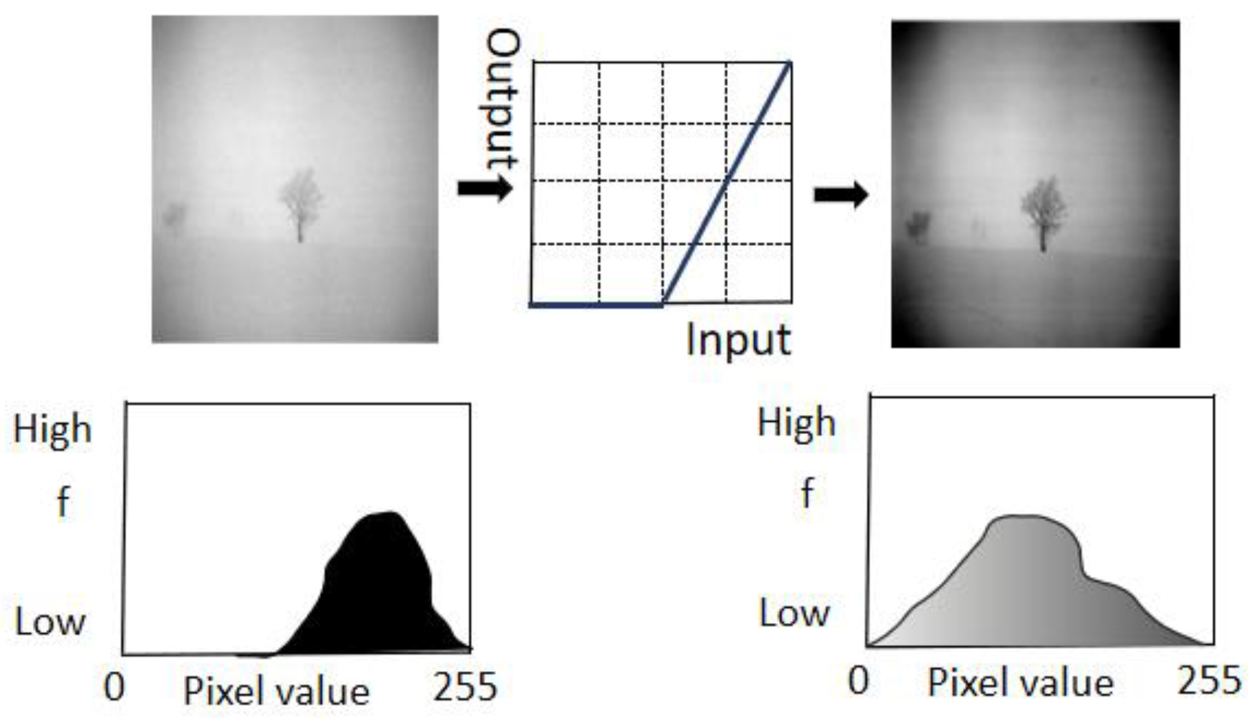
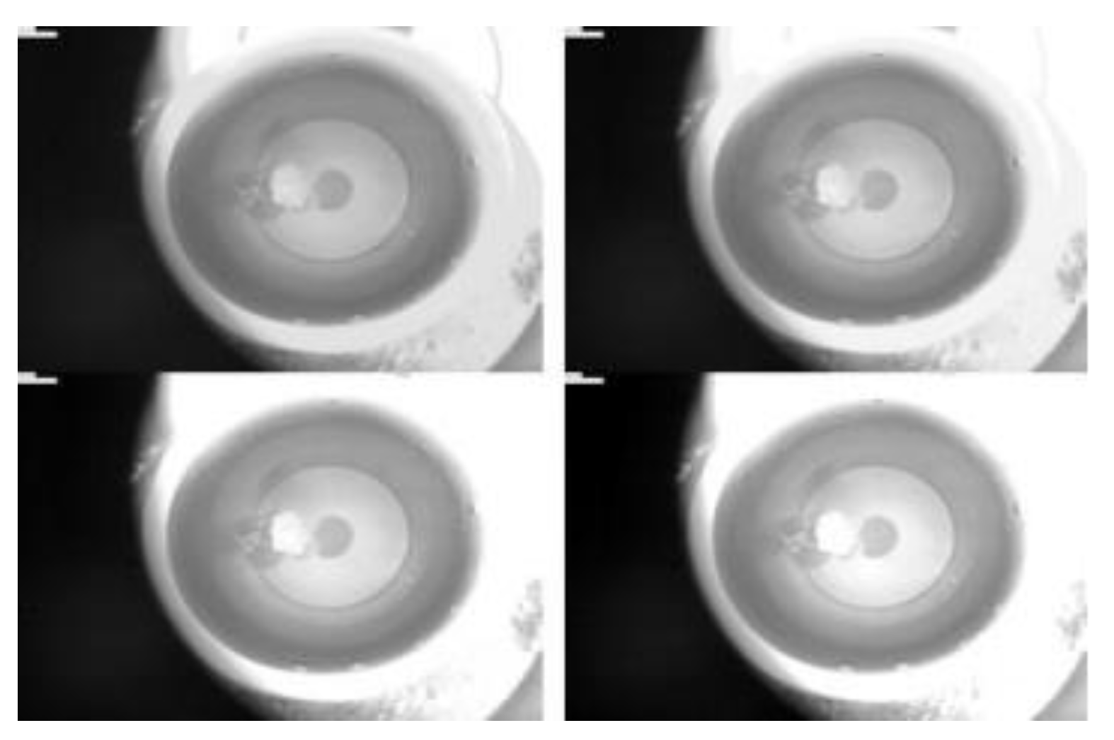
3.1. Image Pre-Processing

Original image: A colour image of the silica is taken by a camera set above the crucible, and a greyscale image can be obtained by completing the image size specification operation and then carrying out greyscale processing. (Processing formula: gray = 0.3r + 0.59 g + 0.11b.)
Grayscale images [13]: The edges of the image are extracted by the Sobel operator and then the image pixel adjustment is applied to the resulting image to obtain a clearer edge. After the above process has been cycled several times, clear edges can be obtained. The number of cycles and the parameters of the pixel adjustment should be slightly modified depending on the image.
Adjustment of image grayscale values [14]: For greyscale images, we can fine-tune the greyscale values so that the image highlights their edges. For the more obvious grey-scale images, we can adjust the pixel values of the image according to a certain mapping relationship, so that the pixel value of the target object is closer to the real situation. Using several more convolutions, we can then detect the clearer edges of Figure 1.
Adjusts the pixel values of the image according to certain mapping relationships. Additionally, the image is grayscale transformed, i.e., the brightness of the grayscale image or the color matrix of the color image is adjusted, where [low_in; high_in] is the grayscale range to be transformed in the original image, and [low_out; high_out] is the grayscale range after the transformation. This mapping relationship allows us to intercept areas of the grey-scale image transformation by adjusting the values of low_in and high_in, and then intercept pixels by adjusting the values of low_out and high_out to obtain a new grey-scale image.
Referring to the first image of the initial gallery, we set low in = 0.02, high in = 0.93, low out = 0, high out = 1. Figure 2 shows four images from one of the loops.
Referring to the first image of the initial gallery, we set low in = 0.02, high in = 0.93, low out = 0, high out = 1. Figure 2 shows four images from one of the loops. Convolution [15]: The method of computing the infinite integral of two functions is called convolution.
y ( n ) = i = x ( i ) h ( n i ) = x ( n ) × h ( n )
The convolution kernel focuses only on local features, and the degree of localization depends on the size of the convolution kernel. Additionally, edge detection with the Sobel operator is essentially a comparison of the similarity of neighboring pixels of an image. When applying convolution on an image, convolution is performed in two dimensions-horizontal and vertical. We mix two buckets of information: the first bucket is the input image. It consists of three matrices-RGB three channels, where each element is an integer between 0 and 255. The second bucket is the convolution kernel, which is a single floating-point matrix. The size and pattern of the convolution kernel can be thought of as a way to stir the image. The output of the convolution kernel is a modified image, often referred to as a feature map in deep learning. there is a feature map for each color channel. The entire pixel value matrix of the image is traversed [16] and the values of the entire pixel value matrix are updated once by the convolution operation. As shown in Figure 3, by changing the dimension and value of the convolution kernel, after a suitable number of convolution operations, we can extract the edges of the image.
Binarization [17]: Binarization is the process of setting the grey scale value of the pixels on an image to 0 or 255, which gives the whole image a distinct black and white effect. Before binarization: the original image is taken to grayscale processing to obtain the grayscale image; the obtained grayscale image is extracted by Sobel operator for edge extraction, and then the image pixel adjustment method is applied to the obtained image, so that clearer edges are obtained. After AI is widely used and the above process is cycled for many times, clear edges can be obtained. The number of cycles and the parameters of pixel adjustment should be slightly modified depending on the image. After that, the resulting image is binarized. After image pre-processing, it is prepared for the determination of the binarization threshold afterwards.
Determination of the binarization threshold [18]: We identify an empirical value as a threshold, which is a key step in obtaining a contour image. Based on the edge images already obtained, in order to outline the crystals, we obtained a negative colour image of the original image, see Figure 4 to add the pixel values of the negative colour image and the edge image. The synthetic image was processed using the binarisation method [19], and all pixel points with pixel values over 200 were set to 255.
The original image needs to be pre-processed before the tracking target is located, and the original image is taken to grey scale to obtain a grey scale image. The resulting grey-scale image is edge extracted by the Sobel operator [20], and then the image pixel adjustment method is applied to the resulting image, so that clearer edges are obtained. After the above process has been cycled several times, a clear edge is obtained. The number of cycles and the parameters of the pixel adjustment should be slightly modified depending on the image. The resulting images were binarised. After image pre-processing, we obtained images with clear edges [21].

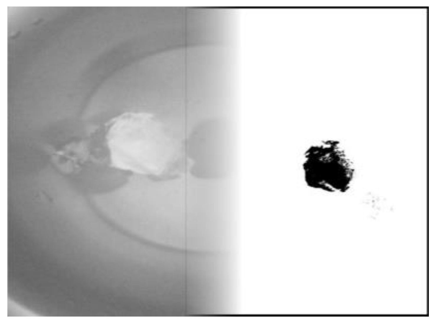
3.2. Indicators of the Trajectory and Edge Profile Characteristics of the Silicon Dioxide Plasmas

Acquisition of silicon dioxide cores [22]: After image pre-processing, we obtained an image with clear edges. Using MATLAB, the image is four connected graphs and the threshold is adjusted, and finally the noise is removed to find the image center of mass coordinates using MATLAB’s own functions, since the given silica time-series image is a two-dimensional plane. Therefore, the mass is replaced by the area. Based on the shape contour of the silica, the centers of mass coordinates are modeled. The following equation is given.
{ m = i = 1 n m i M y = i = 1 n m i × x i , M x = i = 1 n m i × y i x c = M y m , y c = M x m
where the mass m is the sum of all the masses in the point system, M y is the sum of the static moments m i x i is the the y-axis in the mass system, M x is the sum of the static moments m i y i is the x-axis in the mass system, and the coordinates of the centers of the mass are ( x c , y c ) .
Assuming a uniform mass of silica, the center of mass is the center of gravity of the bond. Considering the two-dimensional picture, the area is used instead of the mass to create a mathematical model of the position of the center of mass of the silica particles during the melting process. Using MATLAB software, the position of the center of mass of silica at each moment during the melting process in the high temperature cell was solved as shown in Table 1. After analyzing the relationship between the position of the center of mass and time, we plotted it on a graph. In an image, the units of the coordinate axes are pixels. Relative to the original image, we set the pixels in the top left corner to (1,1), extending to the right for the x-axis and down for the y-axis. We have shown the trajectory of the center of mass from two separate perspectives. In our top view, we mark the change in mass position in steps of 10 points. The trajectory of the center of mass is shown in Figure 5 and Figure 6.
Analysis of the results of Figure 6 and Figure 7 shows that the mass of silica is constantly decreasing during the melting process, and the position of its center of mass is also changing. Mass, one of the key factors in the movement of silica, moves slowly when the mass of silica is large, so the position of the center of mass changes more gently. As time changes, the silica mass becomes smaller, so the movement of the silica becomes violent and the change in the position of the center of mass tends to become progressively more violent.
A correlation analysis of the data from the center of mass [23] was performed and the silica cross-sectional area versus time was calculated in square millimetres for the first 101 images (Figure 7). Additionally, we have precisely calculated the perimeter of the silica melt as a function of time (Figure 8). These properties are a good reflection of the melting properties of the substance, and also the rate at which it melts.

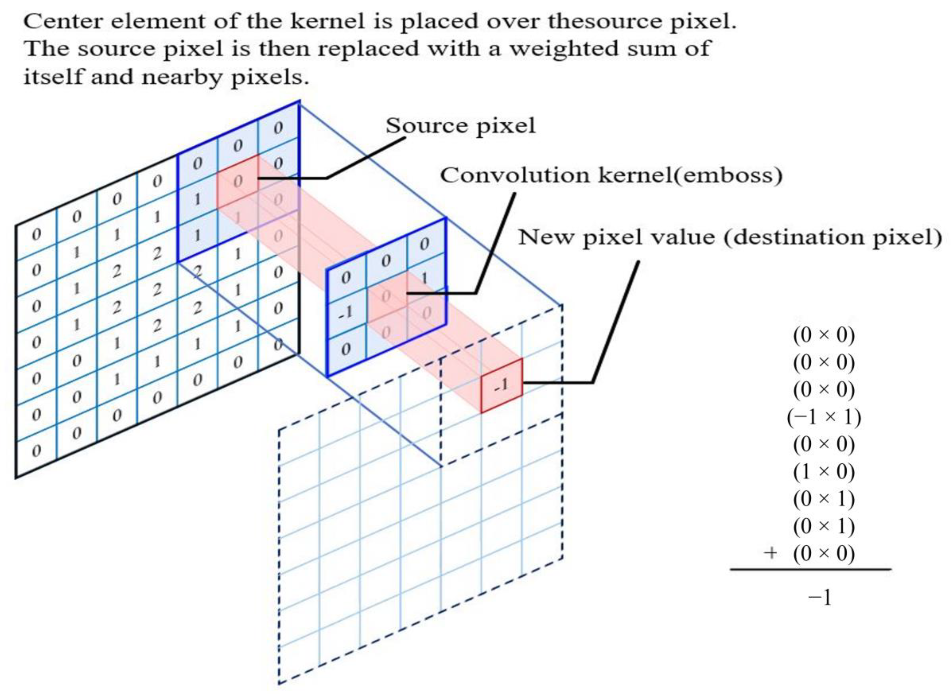
3.3. Theoretical Knowledge of the SFS Model

SFS [24]: By extracting the physical data obtained from the edges, we obtain 2D data. To model the 3D data, we need to find the height value of each pixel point in the plane coordinate system to draw the 3D model. SFS is an algorithm that calculates height values by constructing a relationship between the light source and the image and calculating three important parameters—the inclination angle, the declination angle and the derivative of the image grey scale. Using these three parameters we can calculate the predicted height value. Then, by plotting the calculations we obtain the final result. The flow of the calculation of the melting rate of silicon dioxide particles is shown in Figure 9.
We have obtained physical data such as the position and area of the silica fusion in each image, and to obtain the volume change of the crystals [25], we need to calculate the height value of each pixel point. We established a coordinate system with the plane corresponding to the picture as the xOy plane and the direction of the camera lens as the z-axis, and built a 3D model of the substance based on this coordinate system [26].

3.4. SFS Model Building
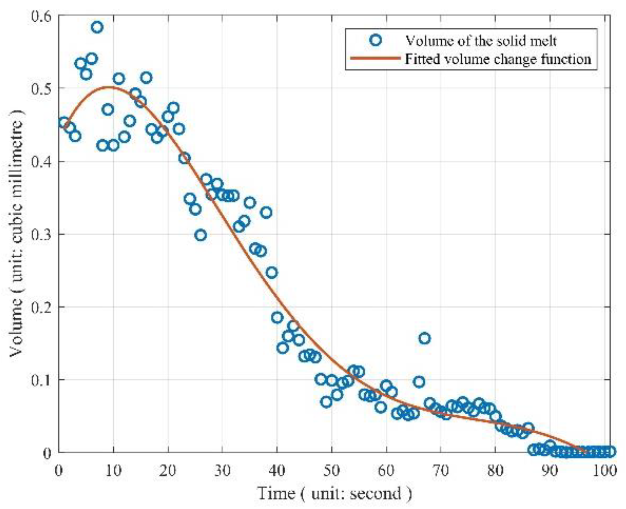
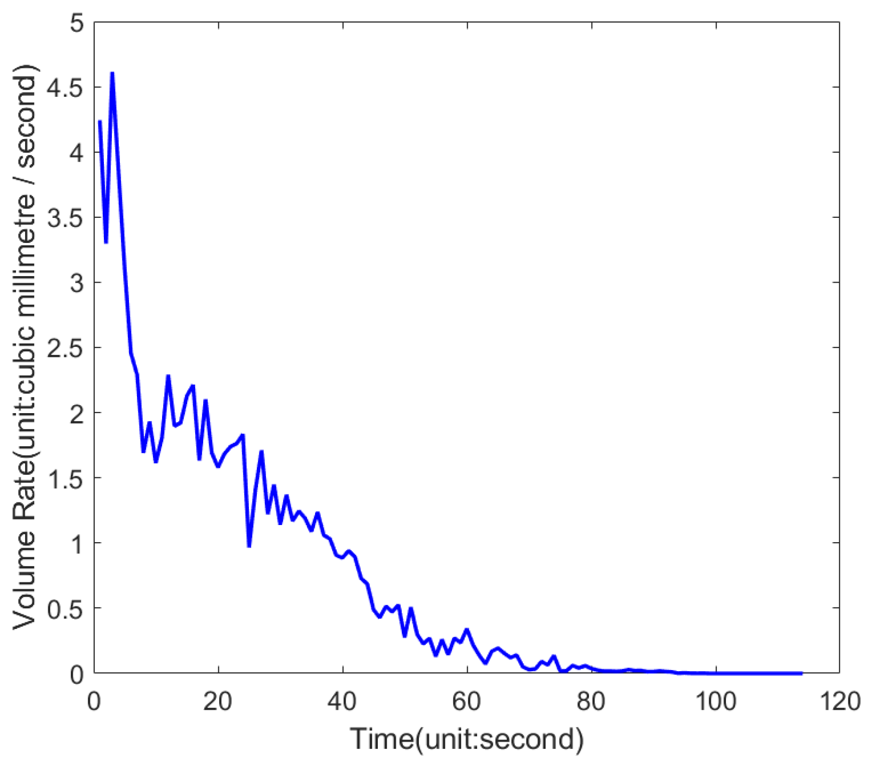
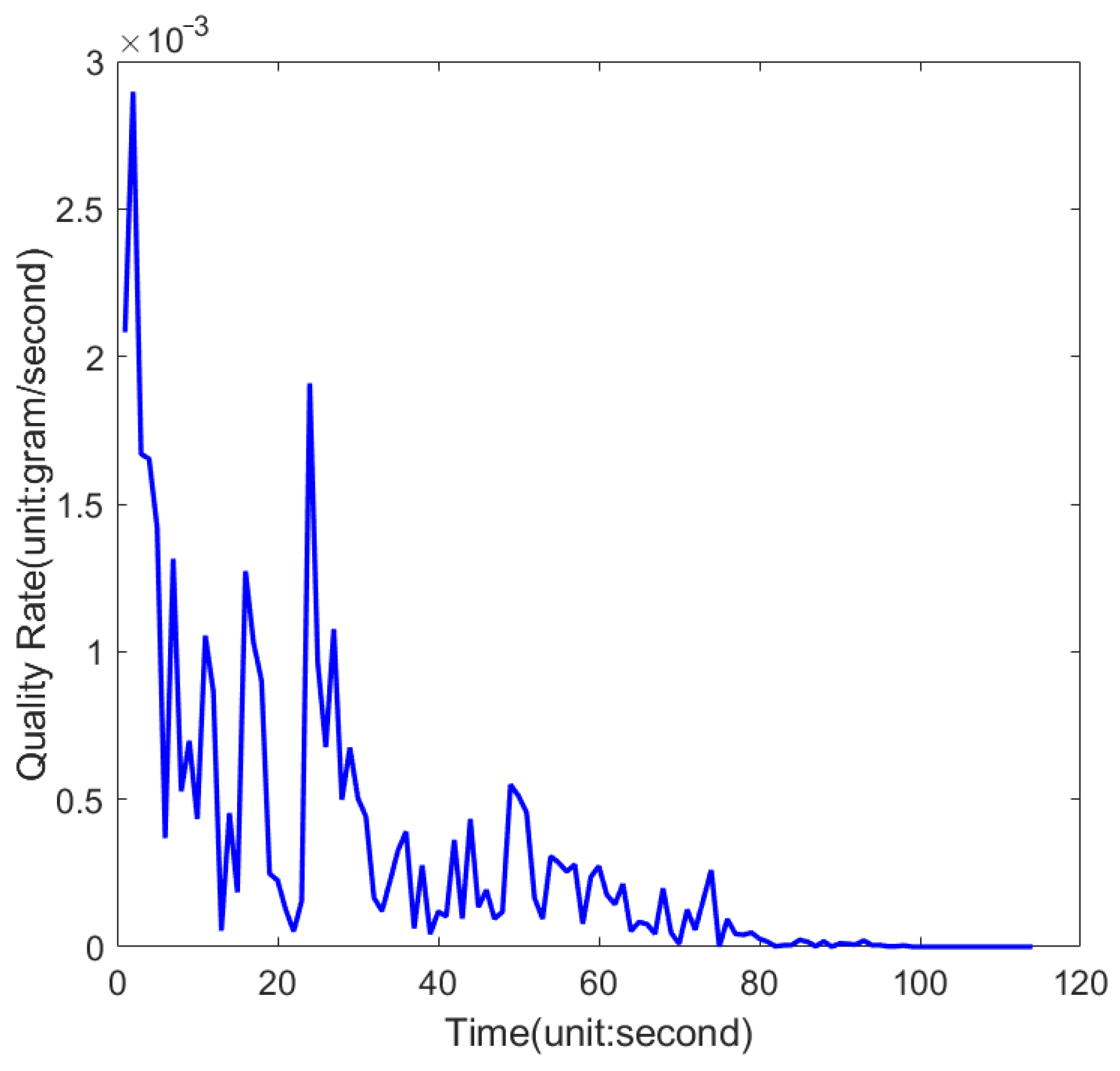
If we assume that the parallel light source is projected into the spherical coordinate system from point P, we can use the inclination ϕ s and declination θ s to plot the position of the light source. The first step is to convert the imaging coordinate system XYZ to the light source coordinate system UVW.
Coordinate conversion [27]: In the spherical coordinate system of Figure 10, a point P on the sphere can be expressed not only in terms of x, y and z coordinates, but also in terms of inclination φ and declination θ . As illustrated in the spherical coordinate system below, keeping the z-axis coordinates constant, we view the coordinate system from the positive direction of the z-axis and the point P is rotated in the XY plane by φ . Keeping the y-axis coordinates constant and viewing the coordinate system from the positive direction of the y-axis, point P is rotated in the XZ plane by φ .
In Equation (3), the transformation equation is coordinated: In the first process, keeping the z-axis constant rotates the XY plane. In the second process, keeping the y-axis constant results in rotation.
( u v w ) = ( cos φ s 0 sin φ s 0 1 0 sin φ s 0 cos φ s ) ( cos θ s sin θ s 0 sin θ s cos θ s 0 0 0 1 ) ( x y z ) = ( cos φ s cos θ s cos φ s sin θ s sin φ s sin θ s cos θ s 0 sin φ s cos θ s sin φ s sin θ s cos φ s ) ( x y z )
Using the transformation matrix R, multiplying it with the original grayscale image, we can obtain the image in the light source coordinate system.
It is assumed that the crystalline surface of the silica satisfies the Lambertian body.
Lambertian [28]: A surface with purely diffuse reflective properties, the brightness of which is uniform when viewed from any angle, is known as a Lambertian reflector. The Lambertian cosine theorem states that the intensity of light reflected from a point on the surface of a Lambertian body is proportional to the cosine of the angle of incidence of the light source at that point.
E = I ρ cos φ
In Equation (4), E is the light intensity of the reflected light. I is the light intensity of the light source. ρ is the reflectance of the surface of the object. φ is the angle between the directional vector of the light source and the normal vector at a point on the surface of the object, which is also the angle of inclination of the surface of the object.
In order to calculate the height value of each pixel, it is necessary to calculate the first order partial derivatives, or bias values, of the image in the x-axis direction and in the y-axis direction. We denote by E x the partial derivative in the x-axis direction and by E y the partial derivative in the y-axis direction.
The Lambert body-based SFS solution algorithm requires the shape of the object surface as an additional constraint from which a regularised mathematical model is built. We apply a local surface approximation to the solution of this problem.
Calculation of grey value bias for images [29]: Assuming that the surface element of a point on the surface of an object is approximated as a point on a sphere, we consider a sphere in the imaging coordinate system; see Equation (5).
z = f ( x , y ) = R 2 x 2 y 2 , R > 0 , R x R , R y R
The partial derivative of f ( x , y ) can be easily found as:
f x = x T 1 2 f y = y T 1 2 , T = R 2 x 2 y 2
The normal vector n at a point on the sphere can be expressed as:
n = ( f x , f y , 1 ) = ( x T 1 / 2 , y T 1 / 2 , 1 )
From the properties of the inclination φ and declination θ of the spherical coordinate system, we can easily derive the vector direction S of the light source as follows:
S = ( sin φ s cos θ s , sin φ s sin θ s , cos φ s )
From the Lambert body cosine theorem, we can calculate as a function of light intensity E:
E = I ρ cos β = I ρ S n | S | | n |   = I ρ x sin φ s cos θ s y sin φ s sin θ s cos φ s T 1 / 2 R
In this way, it is easy to find the partial derivatives of the grey scale values in the x-axis direction, and in the y-axis direction:
{ E x = I ρ R ( sin φ s cos θ s + x cos φ s T 1 / 2 ) E x = I ρ R ( sin φ s cos θ s + y cos φ s T 1 / 2 ) T = R 2 x 2 y 2
Solve for the declination θ and inclination φ of the normal vector at a point on the surface of the object.
The following is conducted for the partial derivatives:
( E x E y ) = ( cos φ s cos θ s cos φ s sin θ s sin θ s cos θ s ) ( E x E y )
In Equation (11) φ s and θ s are the inclination and declination angles of the parallel light sources in the imaging coordinate system. In Equation (11), E x and E y are the partial derivatives of the image grey scale. In Equation (12), the declination θ of a point normal to the surface of the object in the coordinate system of the light source itself has the following relationship:
θ = arctan n y n x
After calculating the bias derivative of the image grey scale in the light source coordinate system from E x and E y , we find the following relationship, which leads to the equation for the declination θ :
θ = arctan n y n x = arctan E y E x
Inclination φ : With reference to the relationship between the imaging coordinate system and the light source coordinate system we know that the inclination angle φ of the normal vector at a point on the surface of an object is the same as the meaning of φ in Lambert’s body cosine theorem. On the whole sphere there must exist a point whose normal vector coincides with the direction vector of the light source, at which point φ = 0, then the grey value of the point is taken to be the maximum value I ρ . Then, with the light source direction vector known, the normal vector of the point with the largest grey value in the image is determined [30]. Let the grey scale value of a point in the image be E i , and it is easy to conclude that:
{ E i = I ρ cos φ i E max = I ρ
Based on the above equation, we conclude the following:
E i E max = cos φ i
The angle of inclination φ normal to a point on the surface of the object in the coordinate system of the light source can then be found by the following equation:
φ i = arccos E i E max
Normal vector: After obtaining the angle of inclination φ and the angle of declination θ in the coordinate system of the light source, we use the formula to calculate the height value z at a point on the surface of the object. Set in the coordinate system of the light source, the normal vector is ( n x , n y , n z ) , then:
( n x , n y , n z ) T = ( l sin φ cos θ , l sin φ sin θ , l cos φ ) T
The normal vectors above are the properties of the object in the light source coordinate system and we need to transform them into the imaging coordinate system to calculate the height values. Based on the previous coordinate transformation matrix, we can invert to obtain the normal vector for each pixel point in the imaging coordinate system:
{ n x = l ( n x cos φ s cos θ s + n y sin φ s + n z sin φ s cos θ s ) n y = l ( n x cos φ s sin θ s + n y cos φ s n z sin φ s sin θ s ) n z = l ( n x sin φ s + n z cos φ s )
where l is the modal length of the normal vector.
Calculating the height value of a pixel point: after finding the normal vector of each pixel point, we need to calculate the height value based on the normal vector. As the normal vector only describes the shape characteristics of the object, we establish a relationship between the normal vector and the height value. The normalised grey value is calculated for each pixel point by the following equation.
G i = n z n x 2 + n y 2 + n z 2 × 255
Among all the grey scale values, there exists a maximum value G max and a minimum value G min , then the height value z of a point on the surface is:
z i = G i G min G max G min

4. Model Analysis

In actual production, the temperature of high-temperature furnaces exceeds 1500 °C Celsius, which leads to the problem of short service life of conventional testing equipment. Since the position of the corundum crucible is fixed, it can be used to establish a two-dimensional coordinate system. In the context of the rapid development of AI, the SFS model is established, which embodies the laws of motion of the object. It is necessary to correct for color and shake problems generated by the Rift Valley CCD system during shooting, 114 images in total. It is clear that the images are part of a benchmark, and we were using them and those images were taken as a part of the experiments. Data filtering is performed on the dataset to remove dirty data. The original image needs to be pre-processed to obtain clearer edges before tracking target localization. After AI is widely used and the above process is cycled for many times, clear edges can be obtained. Additionally, use MATLAB to 4-link the image, adjust the threshold and remove the noise. Finally, the coordinates of the center of mass of the image can be found by using MATLAB’s own functions. On this basis, the target can be better tracked and located, and the trajectory of the center of mass can be drawn accordingly. The area and perimeter of the silica image can be obtained by extracting edge contour features and filling the interior of the contour. The silica volume change in the time series image is calculated after eliminating the effect of background factors. An SFS model is developed to construct a 3D image from the 2D image and calculate the actual melting rate based on the lighting conditions.
The direction of the light source is set to be perpendicular to the plane in which the image is located inward, from which the height value can be calculated for each point on the surface of the object. At this point, the model of the silica melt is reconstructed as shown in Figure 10, so that the melting rate can be calculated.
The above figure shows the process of 3D model reconstruction [31]. Figure 11 shows one of the original images. Figure 10 shows the reconstructed 3D model after using the SFS algorithm. Combining the obtained planar data to do the above processing for each of the 101 images, we obtained the volume change data shown in Table 2.
By fitting the image, we roughly depict the equation of the curve of volume change:
y = ( 5.2488 × 10 10 ) x 5 ( 1.8909 × 10 7 ) x 4 +   ( 2.4295 × 10 5 ) x 3 ( 1.3 × 10 3 ) x 2 + 0.018 x + 0.4269
Neglecting the first two terms, the first-order derivative is found as:
y = ( 7.2885 × 10 5 ) x 2 + 0.0026 x + 0.018
In Figure 12, according to the image analysis, a short expansion process occurs in the crystal from 0–10 s. This process is caused by heating, followed by a gradual melting process. This melting rate is first fast and then slow. The point of change in the melting rate is around 53 s. Thereafter, the volume of the crystal decreases at a slower melting rate until it is completely melted. The faster melting rate is about 0.007 mm3/s. The slower melting rate is around 0.0015 mm3/s.

5. Model Test

Most of the traditional research methods are based on experimental tests. In contrast, this paper adopts a non-contact method with simple operation, high efficiency and low experimental and time costs. Continuous images of iron tailings melting process taken using CCD video recording system were studied at constant temperature. The images were pre-processed. The silica volume changes in the time series images were calculated after eliminating the effects of background factors. A SFS model was developed to construct 3D images from 2D images based on lighting conditions. The actual melting rate was calculated to provide data support for the blast furnace slag direct fiber formation process.
The SFS mathematical model established during the melting of silica was chosen to test the model by the change in volume, mass, perimeter and area of the silica. As can be seen from the figure, the high-temperature melting rate of silica particles is first fast and then slow. Although it is a one-dimensional length and two-dimensional area estimate of the high-temperature melting pattern of silica particles, it is consistent with the actual trend estimated in three-dimensional volume, which can be verified by the visual representation of the sequence images.
Volume and mass: Based on the mathematical knowledge of the collection of lines into a surface, the area is divided into several straight lines in terms of pixel points. Based on the knowledge of the collection of points into lines, the pixel points in each line are summed up using definite integrals and then the average value is found. The average value of the lines can be expressed as the height of the silica. This height is measured in pixels. Based on the actual height of the silica, the volume of the silica at each moment is then examined by combining geometric knowledge. The variation of volume with time is shown in Figure 13. The actual melting rate of silicon dioxide directly reflects the physical quantity of mass. The density of silica is known to be 2.2 g/cm3, and the mass of silica at each moment is obtained and tested. The variation of mass with time is shown in Figure 14.
Volume rate and mass rate: the time interval is 1 s, calculate the difference between volume and mass before and after Δ t time, respectively. The volume and mass change in each unit of time is calculated as the volumetric melting rate and mass change rate of silica. To test this, the volumetric rate change in silica is shown in Figure 15. The mass rate change in silica is shown in Figure 16.
Perimeter: The perimeter of the edge profile pixel at each melting moment of silica and the perimeter of the crucible edge profile pixel were calculated using the program, where the crucible pixel circumference is 1821.7 mm. Based on the crucible diameter of 8, the actual circumference of the crucible is calculated as 25.1327 mm. The actual perimeter of the silica at each moment is then calculated using the ratio of the perimeter of the silica particles to the perimeter of the crucible and the ratio of the silica edge contour pixels to the crucible edge contour pixels, which is then examined; see Figure 17.
Area: Combining the mathematical knowledge of the collection of points in the area into a surface, the pixel area of the graph can be calculated from the pixel points of the graph. Using the program to calculate the pixel area of the picture of silicon dioxide at each moment of melting, the pixel area of the crucible, where the crucible pixel area is 260,684. Based on the crucible diameter of 8mm, the actual area of the crucible is calculated as 50.2655 mm2. The actual area of the silicon dioxide at each moment is examined in this way; see Figure 18.
According to the actual silica melting process, its perimeter, area, volume and mass are decreasing. According to Figure 13, Figure 14, Figure 17 and Figure 18, it can be seen that the experimental results are in accordance with the actual situation and the built SFS model is available. According to Figure 13, Figure 14, Figure 17 and Figure 18, it can be seen that the mass of silica gradually decreases with time. However, the rate of change slows down as time increases, and they have the same trend. The data are decreasing with time, which is in line with the actual situation and the data available for the test of this model using the variation of the selected silica its area. This is in line with the actual situation and the data available for the test of this model using the variation of the selected silica its area.
The melting of silica is positively correlated with the heated surface area. With the change of time, the surface area of heated silica gradually decreases, then the melting rate of silica gradually decreases. According to Figure 15 and Figure 16, which can be seen that the requested silica melting rate is in line with the actual situation and the results are available. The comprehensive analysis shows that the 2D image is constructed into a 3D image and we have established the SFS model according to the lighting conditions, which has a strong practicality. The algorithmic model has strong advantages in both algorithmic simulation and experimental verification and practical application. Therefore, this research result has the value and considerable application prospect to be promoted to other steel companies.

6. Conclusions

In this paper, a non-contact method is used for simple operation, high efficiency and low experimental and time costs. Continuous images of iron tailings melting process taken at constant temperature using a CCD video recording system are studied. The images are pre-processed and the silica volume changes in the time series images are calculated after eliminating the effect of background factors. To construct 3D images from 2D images, an SFS model was developed based on the lighting conditions. The model was tested by selecting the change in volume, mass, perimeter and area of silica. According to the actual situation, during the melting of silica, its perimeter, area, volume, and mass are decreasing. According to the model calculations, it can be seen that they have the same trend of change. The data are decreasing with time, which is in accordance with the actual situation.
The actual melting rate was calculated by analyzing the system simulation results and repeating the experiment accordingly. The melting of silica is positively correlated with the heated surface area. The melting rate of silica decreases with time as the heated surface area of silica decreases. The faster melting rate is about 0.007 mm3/s and the slower melting rate is about 0.0015 mm3/s. This provides data to support the blast furnace slag direct fiber formation process. The introduction of the algorithmic model into the actual production process has certain advantages. Therefore, the SFS model established in this paper has some practical value and is worth promoting in related enterprises.

Author Contributions

L.-J.W. performs algorithm selection and implementation of algorithms in real-world problems. W.-N.M. organizes the data. A.Y. provide methodological guidance. M.T. and J.C. embellished the article. All authors have read and agreed to the published version of the manuscript.

Funding

This research and APC were funded by National Natural Science Foundation of China (NO. 52074126).

Data Availability Statement

For data availability statement, we state that data sharing is not.

Conflicts of Interest

The authors declare no conflict of interest.

References

  1. Bose, B.; Davis, C.R.; Erk, K.A. Microstructural refinement of cement paste internally cured by polyacrylamide composite hydrogel particles containing silica fume and nanosilica. Cem. Concr. Res. 2021, 143, 106400. [Google Scholar] [CrossRef]
  2. Iyer, K.A.; Hu, Y.; Klose, T.; Murayama, T.; Samso, M. Structural characterization of MH/CCD NTD mutations in skeletal ryanodine receptor by cryo-EM. Biophys. J. 2022, 121, 91a–92a. [Google Scholar] [CrossRef]
  3. Li, J.; Liu, W.Q.; Han, Y.; Liu, W.X.; Yang, A.M.; Li, F.; Li, D.L. Dynamic Compensation Model of BF Slag Homogenization Thermal Based on Advanced Deep Learning Algorithm. IEEE Trans. Ind. Inform. 2021, 17, 4107–4116. [Google Scholar] [CrossRef]
  4. Gao, P.; Song, Y.; Song, M.; Qian, P.; Su, Y. Extract nanoporous gold ligaments from SEM images by combining fully convolutional network and Sobel operator edge detection algorithm. Scr. Mater. 2022, 213, 114627. [Google Scholar] [CrossRef]
  5. Yang, A.; Li, S.; Lin, H.; Jin, D. Edge extraction of mineralogical phase based on fractal theory. Chaos Solitons Fractals Interdiscip. J. Nonlinear Sci. Nonequilibrium Complex Phenom. 2018, 117, 215221. [Google Scholar]
  6. Lester, C.; Geonzon, S.M. Accuracy improvement of centroid coordinates and particle identification in particle tracking technique. J. Biorheol. 2019, 33, 2–7. [Google Scholar]
  7. Yang, X.; Lu, D.; Zhu, B.; Sun, Z.; Li, G.; Li, J.; Liu, Q.; Jiang, G. Phase transformation of silica particles in coal and biomass combustion processes. Environ. Pollut. 2022, 292, 118312. [Google Scholar] [CrossRef]
  8. Cao, Y.-L. Research on the Bimetallic Composite Roll Produced by the Electroslag Cladding Method; Northeastern University: Boston, MA, USA, 2018. [Google Scholar] [CrossRef]
  9. Wang, D.-q.; Ma, Z.-j.; Chen, H.; Wang, W.; Zhu, W.C. Thermodynamic analysis of reducing MgO content in slag for blast furnace A in Shougang. China Metall. 2018, 28, issn1006–issn9356. [Google Scholar] [CrossRef]
  10. Han, Y.; Li, J.; Yang, X.-L.; Liu, W.-X. Dynamic Prediction Research of Silicon Content in Hot Metal Driven by Big Data in Blast Furnace Smelting Process under Hadoop Cloud Platform. Complexity 2018, 2018, 1–16. [Google Scholar] [CrossRef]
  11. Li, J.; Wang, J.; Peng, H.; Zhang, L.; Hu, Y.; Su, H. Neural fuzzy approximation enhanced autonomous tracking control of the wheel-legged robot under uncertain physical interaction. Neurocomputing 2020, 410, 342–353. [Google Scholar] [CrossRef]
  12. Narlagiri, L.M.; Rao, S.V. Correction to: Identification of metals and alloys using color CCD images of laser-induced breakdown emissions coupled with machine learning. Appl. Phys. B 2020, 126, 1. [Google Scholar] [CrossRef]
  13. Arora, S.; Chaudhary, N. Gray Image and Colour Image Security using AES Algorithm. IOP Conf.Ser. Mater. Sci. Eng. 2022, 1224, 12024. [Google Scholar] [CrossRef]
  14. Putriany, D.M.; Rachmawati, E.; Sthevanie, F. Indones-ian Ethnicity Recognition Based on Face Image Using Gray Level Co-occurrence Matrix and Color Histogram. IOP Conf. Ser. Mater. Sci. Eng. 2021, 1077, 12040. [Google Scholar] [CrossRef]
  15. Chatterjee, J.; Bhattacharyya, R.; Maulik, A.; Palodhi, K. Application of Machine Learning on sequential deconvolution and convolution techniques for analysis of images from Nuclear Track Detectors (NTDs). Radiat. Meas. 2021, 144, 106581. [Google Scholar] [CrossRef]
  16. Asha, J.; Kamalraj, S. High-capacity reversible data hiding using quotient multi pixel value differencing scheme in encrypted images by fuzzy based encryption. Multimed. Tools Appl. 2021, 80, 1–27. [Google Scholar]
  17. Jacobs, B.A.; Celik, T. Unsupervised document image binarization using a system of nonlinear partial differential equations. Appl. Math. Comput. 2022, 418, 126806. [Google Scholar] [CrossRef]
  18. Mendonça, L.S.M.; Braun, P.X.; Martin, S.M.; Hüther, A.; Mehta, N.; Zhao, Y.; Abu-Qamar, O.; Konstantinou, E.K.; Regatieri, C.V.S.; Witkin, A.J.; et al. Repeatability and Reproducibility of Photoreceptor Density Measurement in the Macula Using the Spectralis High Magnification Module. Ophthalmol. Retin. 2020, 4, 1083–1092. [Google Scholar] [CrossRef] [PubMed]
  19. Sarki, R.; Ahmed, K.; Wang, H.; Zhang, Y.; Ma, J.; Wang, K. Image Preprocessing in Classification and Identification of Diabetic Eye Diseases. Data Sci. Eng. 2021, 6, 11–17. [Google Scholar] [CrossRef]
  20. Ravivarma, G.; Gavaskar, K.; Malathi, D.; Asha, K.G.; Aarthi, S. Implementation of Sobel operator based image edge detection on FPGA. Mater. Today Proc. 2021, 45, 2401–2407. [Google Scholar] [CrossRef]
  21. Vafa, A.P.; Karimi, P.; Khavasi, A. Analog optical edge detection by spatial high-pass filtering using litho-graphyfree structures. Opt. Commun. 2021, 495, 127084. [Google Scholar] [CrossRef]
  22. Ortega, P.P.P.; Ortiz, O.R.D.; Marin, R.A.M. Hyperbolic Center of Mass for a System of Particles in a Two-Dimensional Space with Constant Negative Curvature: An Application to the Curved 2-Body Problem. Mathematics 2021, 9, 531. [Google Scholar] [CrossRef]
  23. Girdhar, G.L.; Ravi, K.S.P. An efficient distance estimation and centroid selection based on k-means clustering for small and large dataset. Int. J. Adv. Technol. Eng. Explor. 2020, 7, 234–240. [Google Scholar]
  24. Chaurasia, V.; Pandey, M.K.; Pal, S. Prediction of Presence of Breast Cancer Disease in the Patient using Machine Learning Algorithms and SFS. IOP Conf. Ser. Mater. Sci. Eng. 2021, 1099, 12003. [Google Scholar] [CrossRef]
  25. Toda, A.; Taguchi, K.; Nozaki, K. Fast limiting behavior of the melting kinetics of polyethylene crystals examined by fast-scan calorimetry. Thermochim. Acta 2019, 677, 211–216. [Google Scholar] [CrossRef]
  26. Mahrous, A.; Elgreatly, A.; Qian, F.; Schneider, G.B. A comparison of pre-clinical instructional technologies: Natural teeth, 3D models, 3D printing, and augmented reality. J. Dent. Educ. 2021, 85, 1795–1801. [Google Scholar] [CrossRef]
  27. Sahlstrom, T.; Pulkkinen, A.; Leskinen, J.; Tarvainen, T. Computationally Efficient Forward Operator for Photoacoustic Tomography Based on Coordinate Transformations. IEEE Trans. Ultrason. Ferroelectr. Freq. Control. 2021, 68, 2172–2182. [Google Scholar] [CrossRef]
  28. Kim, H.J.; Kim, W.; Cho, H. Lambertian Extraction of Light from Organic Light-Emitting Devices Using Randomly Dispersed Sub-Wavelength Pillar Arrays. J. Nanosci. Nanotechnol. 2021, 21, 3909–3913. [Google Scholar] [CrossRef]
  29. Kang, K.; Kushnarev, S.; Pin, W.W.; Ortiz, O.; Shihang, J.C. Impact of Virtual Reality on the Visualization of Partial Derivatives in a Multivariable Calculus Class. IEEE Access 2020, 8, 58940–58947. [Google Scholar] [CrossRef]
  30. Davids, P.S. Normal vector approach to Fourier modal scattering from planar periodic photonic structures. Photonics Nanostructures Fundam. Appl. 2021, 43, 100864. [Google Scholar] [CrossRef]
  31. Brambach, M.; Ernst, A.; Nolbrant, S.; Drouin-Ouellet, J.; Kirkeby, A.; Parmar, M.; Olariu, V. Neural tube patterning: From a minimal model for rostrocaudal patterning toward an integrated 3D model. iScience 2021, 24, 102559. [Google Scholar] [CrossRef]
Figure 1. Image greyscale adjustment—fine tuning of greyscale values.
Minerals 12 01286 g001
Figure 2. Image with adjusted grayscale values.
Minerals 12 01286 g002
Figure 3. Convolution operation corresponding to the pixel value matrix of the silicon dioxide image.
Minerals 12 01286 g003
Figure 4. Image pre-processing—binarisation.
Minerals 12 01286 g004
Figure 5. Trajectory of the center of mass during the melting of silicon dioxide.
Minerals 12 01286 g005
Figure 6. Position of the center of mass during the melting of silicon dioxide.
Minerals 12 01286 g006
Figure 7. Silicon dioxide during melting in a hot cell plot of area change at each moment.
Minerals 12 01286 g007
Figure 8. Silicon dioxide during melting in a hot cell change in circumference at each moment.
Minerals 12 01286 g008
Figure 9. Flow chart for calculating the melting rate of silicon dioxide particles.
Minerals 12 01286 g009
Figure 10. Reconstructing 3D models of silica crystals using the SFS algorithm.
Minerals 12 01286 g010
Figure 11. Original color image of silicon dioxide.
Minerals 12 01286 g011
Figure 12. Trend of silicon dioxide melting rate with time.
Minerals 12 01286 g012
Figure 13. Volume change of silicon dioxide at each moment during the melting process in the high-temperature cell.
Minerals 12 01286 g013
Figure 14. Graph of the mass change of silicon dioxide at each moment during the melting process in the high-temperature cell.
Minerals 12 01286 g014
Figure 15. Volume rate variation of silicon dioxide at each moment during high-temperature cell melting.
Minerals 12 01286 g015
Figure 16. Graph of the change in mass rate of silicon dioxide at each moment during the melting process in the temperature cell.
Minerals 12 01286 g016
Figure 17. Variation of the perimeter of silicon dioxide at each moment during the melting process in the high-temperature cell.
Minerals 12 01286 g017
Figure 18. Area change of silicon dioxide at each moment during high-temperature cell melting.
Minerals 12 01286 g018
Table 1. Position of the center of mass at each moment during the melting of silicon dioxide in a hot cell.
MomentCoordinate PointsMomentCoordinate Points
1(225, 202)25(209, 223)
2(224, 205)26(208, 212)
3(217, 226)27(191, 232)
4(220, 225)28(176, 246)
5(213, 244)29(171, 241)
6(236, 235)30(166, 242)
7(221, 239)31(164, 245)
8(218, 235)32(161, 243)
9(215, 235)33(165, 244)
10(214, 234)34(168, 240)
11(214, 237)35(176, 244)
12(209, 239)36(169, 239)
13(208, 236)37(198, 233)
14(204, 233)38(193, 234)
15(197, 237)39(195, 228)
16(281, 225)40(190, 236)
17(203, 239)41(171, 245)
18(200, 237)42(164, 240)
19(199, 237)43(156, 245)
20(195, 234)44(142, 250)
21(198, 233)45(139, 253)
22(190, 237)46(140, 249)
23(191, 234)47(136, 253)
24(202, 231)48(126, 265)
Table 2. Table of actual melting rates of silicon dioxide by volume.
MomentVolume
(mm3)
Rate
(mm3/s)
MomentVolume
(mm3)
Rate
(mm3/s)
14.240.95250.970.44
23.301.32261.400.31
34.610.76271.710.49
43.850.75281.220.23
53.100.65291.450.31
62.460.17301.140.23
72.290.60311.370.20
81.690.24321.170.08
91.930.32331.250.06
101.610.20341.190.10
111.810.48351.090.15
122.290.39361.240.18
131.900.02371.060.03
141.920.21381.030.13
152.130.08390.910.02
162.210.58400.890.05
171.630.47410.940.04
182.100.41420.890.16
191.690.11430.730.04
201.580.10440.690.20
211.680.06450.490.06
221.740.02460.430.09
231.760.07470.520.04
241.830.87480.470.05
Publisher’s Note: MDPI stays neutral with regard to jurisdictional claims in published maps and institutional affiliations.

