Towards Consistent Interpretations of Coal Geochemistry Data on Whole-Coal versus Ash Bases through Machine Learning

Xu, Na; Peng, Mengmeng; Li, Qing; Xu, Chuanpeng

doi:10.3390/min10040328

Open AccessArticle

Towards Consistent Interpretations of Coal Geochemistry Data on Whole-Coal versus Ash Bases through Machine Learning

¹

College of Geoscience and Survey Engineering, China University of Mining and Technology (Beijing), Beijing 100083, China

²

Department of Computing, Hong Kong Polytechnic University, Hung Hom, Kowloon, HKSAR, Hong Kong, China

^*

Author to whom correspondence should be addressed.

Minerals 2020, 10(4), 328; https://doi.org/10.3390/min10040328

Submission received: 18 March 2020 / Revised: 4 April 2020 / Accepted: 6 April 2020 / Published: 7 April 2020

(This article belongs to the Collection Critical Metals and Minerals in Coal and Coal Combustion Products)

Download

Browse Figures

Versions Notes

Abstract

:

Coal geochemistry compositional data on whole-coal basis can be converted back to ash basis based on samples’ loss on ignition. However, the correlation between the concentrations of elements reported on whole-coal versus ash bases in many cases is inconsistent. Traditional statistical methods (e.g., correlation analysis) for compositional data on both bases may sometimes result in misleading results. To address this issue, we hereby propose an improved additive log-ratio data transformation method for analyzing the correlation between element concentrations reported on whole-coal versus ash bases. To verify the validity of the method proposed in this study, a data set which contains comprehensive analyses of 106 Late Paleozoic coal samples from the Datanhao mine and Adaohai Mine, Inner Mongolia, China, is used for the validity testing. A prediction model was built for performance evaluation of two methods based on the hierarchical clustering algorithm. The results show that the improved additive log-ratio is more effective in prediction for occurrence modes of elements in coal than the previously reported stability method, and therefore can be adopted for consistent interpretations of coal geochemistry compositional data on whole-coal vs. ash bases.

Keywords:

whole-coal basis; ash basis; correlation; hierarchical clustering algorithm; prediction

1. Introduction

The modes of occurrence of elements in coal are important because: (1) the release of toxic elements from coal are, in part, dependent on the hosts of these elements [1,2,3,4,5]; (2) they provide insights into the sources of mineral matter in coal, which result from different geological processes [1,6,7]; (3) the technologies designed for critical metals recovery from coal and coal ash largely depend on the modes of occurrence of these elements [8,9,10]; and (4) the modes of occurrence of an element can play an important role in determining the technological behavior of the element [1]. In addition to a number of physical and chemical analyses that have been used for determining the modes of occurrence in coal [11,12], some statistical methods have been commonly adopted to investigate the hosts of both major and trace elements in coal. Correlation analysis of element concentrations vs. ash yields is the simplest method that has been widely used in such studies [1]. Concentrations of elements in coal are usually reported on two bases: whole-coal and ash bases. The element concentrations in an ash basis can be converted back to those in a whole-coal basis based on ash yields (or loss on ignition), using the formula:

{[E_{i}]}_{c o a l} = ({[E_{i}]}_{a s h} \times a s h yield)

, or vice versa; where

E_{i}

, ash, and coal represent element concentration, ash basis and whole-coal basis respectively.

Element concentrations with a positive correlation with ash yields, indicate a dominant inorganic association. A negative correlation of element concentration with ash yield implies a possible organic association [13,14].

However, it has been found that, in many cases, the modes of occurrence of elements in coal based on correlations between element concentration and ash yield are not consistent in terms of the two bases [13,15,16]. For example, the correlation coefficients between the element concentrations and ash yields in the Pennsylvanian coals in the Datanhao and Adaohai mines in Inner Mongolia, China, are not consistent in terms of the two bases [13,15], and, consequently, different modes of occurrence of the elements are inferred. Geboy et al. [16] showed that this inconsistency is attributable to the nature of the elemental concentrations, i.e., compositional data. The sum of major and trace elements in coal is expected to be 100% in an ash basis; however, if based on a whole-coal basis, the sum of elemental concentrations (not including organic C, H, N, and S) plus loss on ignition (LOI, LOI% = 100% − ash yield%) is expected to be 100%. In particular, the sum of the concentrations of all elements plus LOI is 100% (whole-coal basis) from the Datanhao coal mine, Daqingshan Coalfield, Inner Mongolia, northern China [13,15].

Most related literature regarding statistical analysis of compositional data calculated is based on Aitchison [17]. For compositional data pertaining to the non-Euclidean space, the statistical analysis in the Euclidean space for coal geochemistry data may result in misleading conclusions. The cause for the correlation difference of elemental concentrations is attributed to sub-compositional incoherence. In order to fully understand the coal compositional data and then more accurately reveal the modes of occurrence of elements based on statistical analysis, coal compositional data need to be first transformed from non-Euclidean space to Euclidean space. As described below, a log-ratio transformation has been proposed to address the incoherence paradox of coal compositional data reported on different bases.

2. Compositional Data Transformation

In general, compositional data transformation can be performed in three ways: additive log-ratio transformation, centered log-ratio transformation, and isometric log-ratio transformation.

2.1. Additive Log-Ratio (alr) Transformation

All the coal geochemistry compositional data

X

of

D

part with positive components can be expressed as

X = (x_{1}, \dots, x_{D}) : x_{1} + \dots + x_{D} = 1

. The coal geochemistry compositional data can be mapped from simplex space

S

to Euclidean space

R

, and the result for an observation

x_{i} \in S

can be transformed into

y_{i} \in R

. For the coal geochemistry compositional data, alr transformation [18] is defined as

y_{i} = a l r (x_{i}) = (l n \frac{x_{1}}{x_{j}}, \dots, l n \frac{x_{j - 1}}{x_{j}}, l n \frac{x_{j + 1}}{x_{j}}, \dots, l n \frac{x_{D}}{x_{j}})

, where

x_{j}

is a subjective element in coal.

2.2. Centered Log-Ratio (clr) Transformation

For solving subjective characteristics of additive log-ratio data transformation, clr [18] data transformation is proposed. For the coal geochemistry compositional data, clr transformation is defined as

y_{i} = c l r (x_{i}) = (l n \frac{x_{i}}{\sqrt[D]{\prod_{j = 1}^{D} x_{j}}}), i = 1, \dots, D - 1

From the clr transformation view, all the coal geochemistry compositional data can be obtained by log transformation, and thus the result observation is centered.

2.3. Isometric Log-Ratio (ilr) Transformation

The isometric log-ratio (ilr) [19] coordinates aim at building an orthonormal basis in the hyperplane. In particular, ilr coordinates set up an orthonormal basis in the hyperplane formed by clr coefficients, and ilr can avoid the singularity occurred with clr coefficients. For the coal geochemistry compositional data, ilr transformation is defined as

y_{i} = i l r (x_{i}) = (\sqrt{\frac{i}{i + 1}} l n \frac{\sqrt[i]{\prod_{j = 1}^{i} x_{j}}}{x_{i + 1}}), i = 1, \dots, D - 1

.

To solve the problem of consistent correlations whether using ash or whole-coal bases, Geboy et al. [16] proposed the notion of stability between two different elements as a bivariate measure based on ilr transformation [19]. While they have shown that the stability between two elements is identical regardless of the reporting basis [16], the stability may seem less illuminating than the correlation coefficient.

In the next section, we propose an improved additive log-ratio data transformation to calculate the correlation between transformed element concentrations. In comparison with other methods, the improved additive log-ratio method is based on the geochemical properties, e.g., the immobility of Zr and Al. Additionally, the method is elegant in predicting the occurrence modes of elements in coal. The results show that the correlation is identical regardless of whole-coal basis or ash basis. Our purpose is to compare the prediction for the mode of occurrence between the improved additive log-ratio data transformation and the stability method [16], by using the hierarchy clustering algorithm [20].

3. Improved Additive Log-Ratio and Correlation Analysis

The improved additive log-ratio transformation for coal element data is proposed based on additive log-ratio transformation.

3.1. Improved Additive Log-Ratio Transformation

For the coal geochemistry trace elements compositional data, the improved additive log-ratio (ialr) can be defined as

y_{i} = i a l r (x_{i}) = (l n \frac{x_{1}^{0}}{x_{j}^{0}}, \dots, l n \frac{x_{i - 1}^{0}}{x_{j}^{0}}, l n \frac{x_{i + 1}^{0}}{x_{j}^{0}}, \dots, l n \frac{x_{D}^{0}}{x_{j}^{0}})

(1)

Here,

x_{j}

can be assigned with Zr because Zr is a stable element during peat accumulation, diagenetic and epigenetic processes relative to other trace elements. The log ratio between the trace elements

x_{i}^{0}

and Zr is

l n \frac{x_{i}^{0}}{Z r}

.

For the coal geochemistry major elements compositional data, the improved additive log-ratio (ialr) can be defined as

y_{i} = i a l r (x_{i}) = (l n \frac{x_{1}^{1}}{x_{j}^{1}}, \dots, l n \frac{x_{i - 1}^{1}}{x_{j}^{1}}, l n \frac{x_{i + 1}^{1}}{x_{j}^{1}}, \dots, l n \frac{x_{D}^{1}}{x_{j}^{1}})

(2)

Here,

x_{j}

can be assigned with Al₂O₃ because aluminum is a stable element during peat accumulation, diagenetic and epigenetic processes relative to other major elements (such as Na, Mg, Si, K, Ca) [21,22,23,24,25,26,27,28,29,30], although Al is somewhat mobile in some very specific geological conditions [11,25]. The log-ratio between the major elements

x_{i}^{1}

and Al₂O₃ is

l n \frac{x_{i}^{1}}{A l_{2} O_{3}}

.

3.2. Correlation Analysis of Different Transformation Methods

The correlation coefficients between the concentrations of elements and ash yields can be quite different in terms of the former on ash or whole-coal bases. All the coal geochemistry data (which are shown in the Table 1, Table 2, Table 3, Table 4, Table 5, Table 6, Table 7 and Table 8) can be transformed by using some data transformation methods, in particular, the improved alr, clr [18] and ilr [19]. Based on closely related literature, the common data transformation methods for composition data from non-Euclidean space to Euclidean space are alr, clr and ilr. Clr is much better than alr in solving subjective characteristics of additive log-ratio data transformation, while ilr is much better than clr in avoiding the singularity occurred with clr coefficients. The improved alr is the new data transformation method proposed in this paper. Among all the transformed coal geochemistry elements data, the correlations between different element concentrations can be estimated. The correlation between different element concentrations based on our proposed improved alr is the same, regardless of ash or whole-coal bases.

Elemental concentrations based either on ash basis or on whole-coal basis have been reported by a number of authors [31,32,33,34,35,36], and either reported basis is correct, because the concentrations of elements in coal ash can be converted back to the whole-coal basis by using the equation

{[E_{i}]}_{c o a l} = ({[E_{i}]}_{a s h} \times a s h %)

. The transformed data with improved alr on whole-coal and ash bases can be described as

i a l r {(X)}_{w c} = i a l r {(X)}_{a s h} .

The transformed coal element data with clr on whole-coal and ash bases can be described as

c l r {(X)}_{w c} = c l r {(X)}_{a s h}

. The transformed coal element data with ilr on whole-coal and ash bases can be described as

i l r {(X)}_{w c} = i l r {(X)}_{a s h}

.

3.3. Correlation Replaced by Stability

In Geboy et al.’s method [16], all the coal geochemistry compositional data follow the ilr transformation method. Then the stability

s t a b (x_{i}, x_{j}) = e x p (- v a r (i l r (x_{i}, x_{j})))

between different elements, which is called bivariate measure, was proposed.

Geboy et al.’s experiments [16] proved that the stability between different element concentrations is identical, regardless of the reporting basis. The application of the proposed stability, similar to correlation, has solved the inconsistency problem of the coal geochemical data reported on different bases.

Table 1, Table 2, Table 3, Table 4, Table 5, Table 6, Table 7 and Table 8 show all the correlations and stability [37] between element concentrations for the Adaohai mine and the Datanhao mine, using different data transformation methods based on ash and whole-coal bases. Our improved alr for correlation is consistent regardless of the different reporting bases. The stability proposed by Geboy et al. [16] between element concentrations, which is similar to correlation, demonstrates the consistency regardless of using different reporting bases.

4. Prediction for Occurrence Mode of Element in Coal Based on Hierarchy Clustering

To verify the performance of the transformation methods for coal geochemistry compositional data, a prediction model for the mode of occurrence of coal element data was built based on the hierarchical clustering algorithm. The element

x_{i}

of the coal geochemistry was selected as a feature for clustering analysis.

4.1. Hierarchical Clustering

Belonging to unsupervised machine learning, hierarchical hierarchy clustering is a basic method with broad applications in different fields [20]. It divides unlabeled data into different clusters according to their similarity. Data points are clustered together if their nature is similar and those with dissimilar nature are assorted into different clusters.

For improving the working effect, the hierarchical clustering algorithm [20] is used to measure the similarity between different groups of data features. As the name suggests, it produces hierarchical representations in which the clusters at each level of the hierarchy are created by merging clusters at the next lower level. At the lowest level, each cluster contains a single feature. At the highest level, there is only one cluster containing all the features.

Existing strategies for hierarchical clustering can be divided into two basic paradigms: agglomerative and divisive [20]. For our work, the agglomerative strategy is used. The agglomerative strategy starts from the bottom, and at each level it recursively merges a selected pair of clusters into a single cluster. This produces a grouping at the next higher level with one less cluster, and the pair chosen for merging consists of the two clusters with the smallest inter-group dissimilarity. The entire hierarchy represents the ordered sequence of clusters containing all the coal elements.

4.2. Similarities Analysis between the Elements in Coal

There are two popular methods used to measure the data similarity: one is based on the distance and the other is based on the correlation coefficient. Distance-based similarity states that two data points with a small distance should have a large similarity, whereas correlation-based similarity state that two data points with a large correlation should have a large similarity [38]. Let a weighted graph

G (V, E, ω)

be a similarity graph [20]. The node

V (x_{i})

of the graph

G

represents an element. The edge

E (x_{i,} x_{j})

represents the relationship between two different elements, and

ω

represents the similarity of the different elements. The similarity for the coal geochemistry element is expressed as

d_{k} (x_{i k,} x_{j k}) = \sum_{k = 1}^{p} d_{k} (x_{i k,} x_{j k}) = \sum_{k = 1}^{p} \frac{\sum_{k} (x_{i k} - \bar{x_{i}}) (x_{j k} - \bar{x_{j}})}{\sqrt{\sum_{k} {(x_{i k} - \bar{x_{i}})}^{2} \sum_{k} {(x_{j k} - \bar{x_{j}})}^{2}}}

. Additionally, the stability given by Geboy is used for the similarity between elements in coal, i.e.,

d_{k} (x_{i,} x_{j}) = s t a b (x_{i}, x_{j}) = e x p (- v a r (i l r (x_{i}, x_{j})))

. Furthermore, the similarities graph G for the coal geochemistry compositional data can be expressed as

G (V, E, ω) = G (V (x_{i}), E (x_{i,} x_{j}), d_{k} (x_{i,} x_{j}))

.

4.3. Agglomerative Clustering Algorithm for Prediction

While agglomerative clustering is a mainstream clustering method that can produce an informative hierarchical structure of clusters, the results of agglomerative clustering highly depend on data similarity. Agglomerative clustering starts with every feature representing a single cluster. At each of the N-1 steps, the closest two clusters are merged into a single cluster, producing one less cluster at the next higher level. Following [20], the measure of similarity between element in coal clusters is defined as

d_{k} (x_{i k,} x_{j k})

.

Each level of the hierarchy represents a particular grouping of the element features into disjoint clusters. Recursive binary agglomerative can be presented by a binary tree. The nodes of the trees represent all the elements in coal. The N terminal nodes represent N individual elements. Each nonterminal node has two child nodes. Agglomerative clustering merges the child nodes representing two different clusters to form a parent node. The binary tree is plotted so that the height of each node is proportional to the value of the intergroup similarity between the children. The terminal nodes representing individual element features are all plotted at zero height. This type of graphical display is called a dendrogram [20].

Let

I and J

represent two clusters. The similarity between

I and J

d_{k} (x_{i k} \in I, x_{j k} \in J)

is computed from the set of pairwise feature similarities, where one feature of the pair

i

is in the cluster

I

and the other

j

in the cluster

J

. Besides average linkage, single linkage, complete linkage, centroid and ward are common clustering approaches. For centroid and ward clustering, they are usually used for distance-based similarity, not correlation-based similarity. After the experiments for describing the occurrence modes of elements in coal in the real coal element dataset of the Datanhao mine and the Adaohai mine [13,15], average linkage agglomerative clustering is much better than for the other two clustering approaches overall. Therefore, the average linkage agglomerative clustering algorithm is used for prediction of the occurrence modes of elements in coal in this paper. Average linkage agglomerative clustering algorithm uses the average similarity between the clusters as shown in Table 9. It is expressed as

d_{k} (x_{i} \in I, x_{j} \in J) = \frac{\sum d_{k} (x_{i} \in I, x_{j} \in J)}{N_{I} N_{J}}

, where

N_{I} and N_{J}

are the respective numbers of the features in each group. The average linkage agglomerative clustering algorithm for prediction of the occurrence modes of elements in coal is executed on the real coal element dataset of the Datanhao mine and the Adaohai mine [13,15].

5. Results

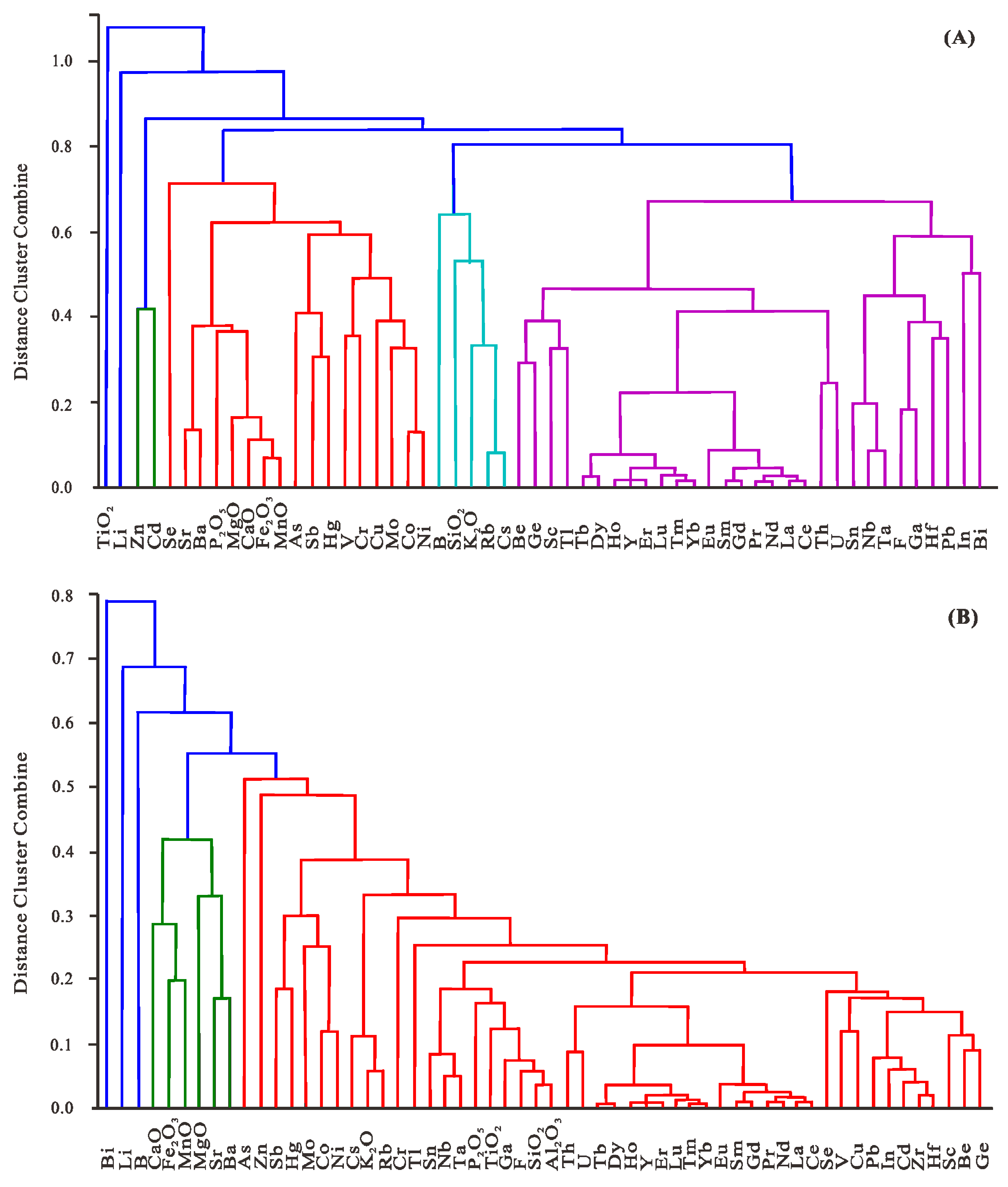
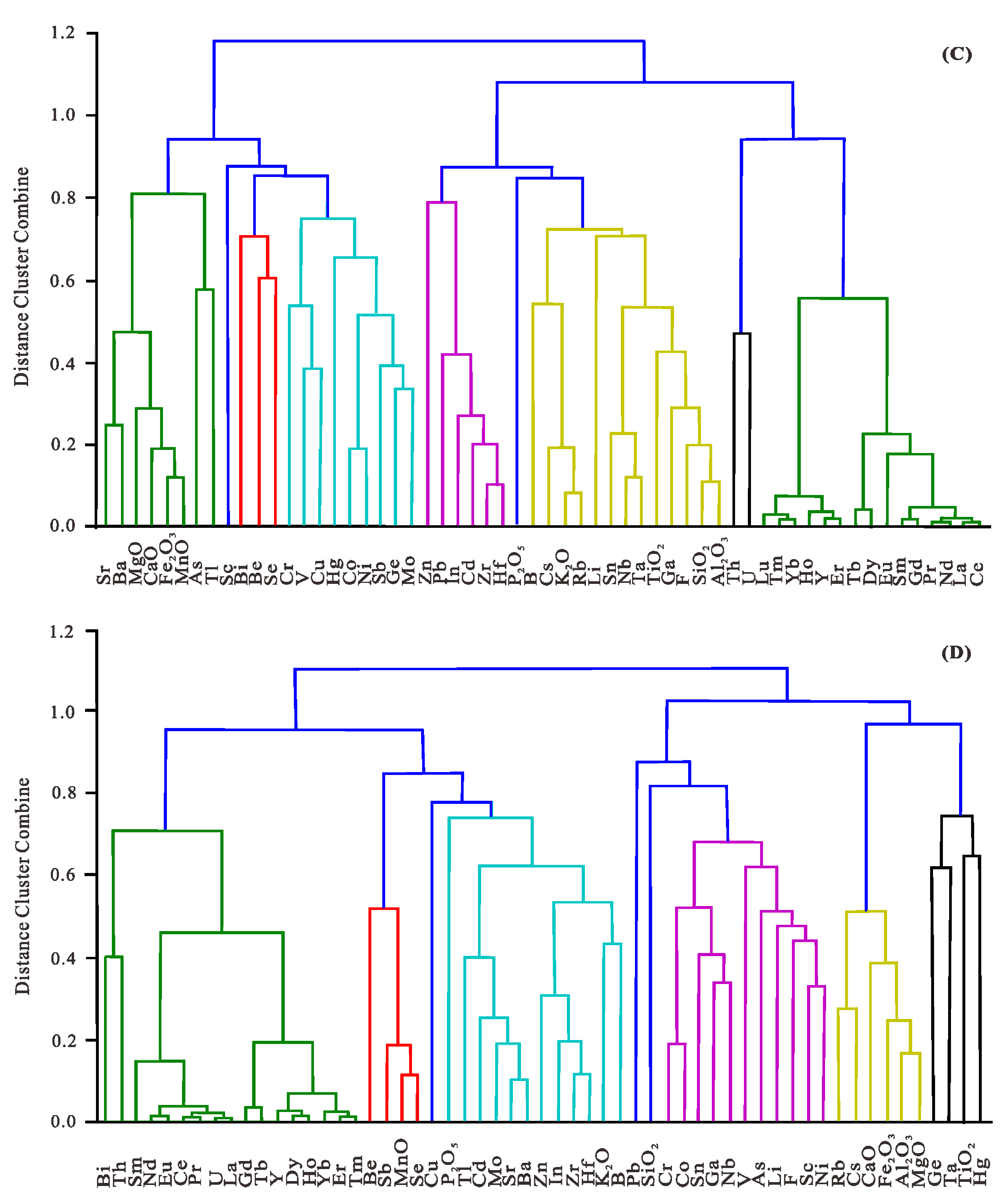
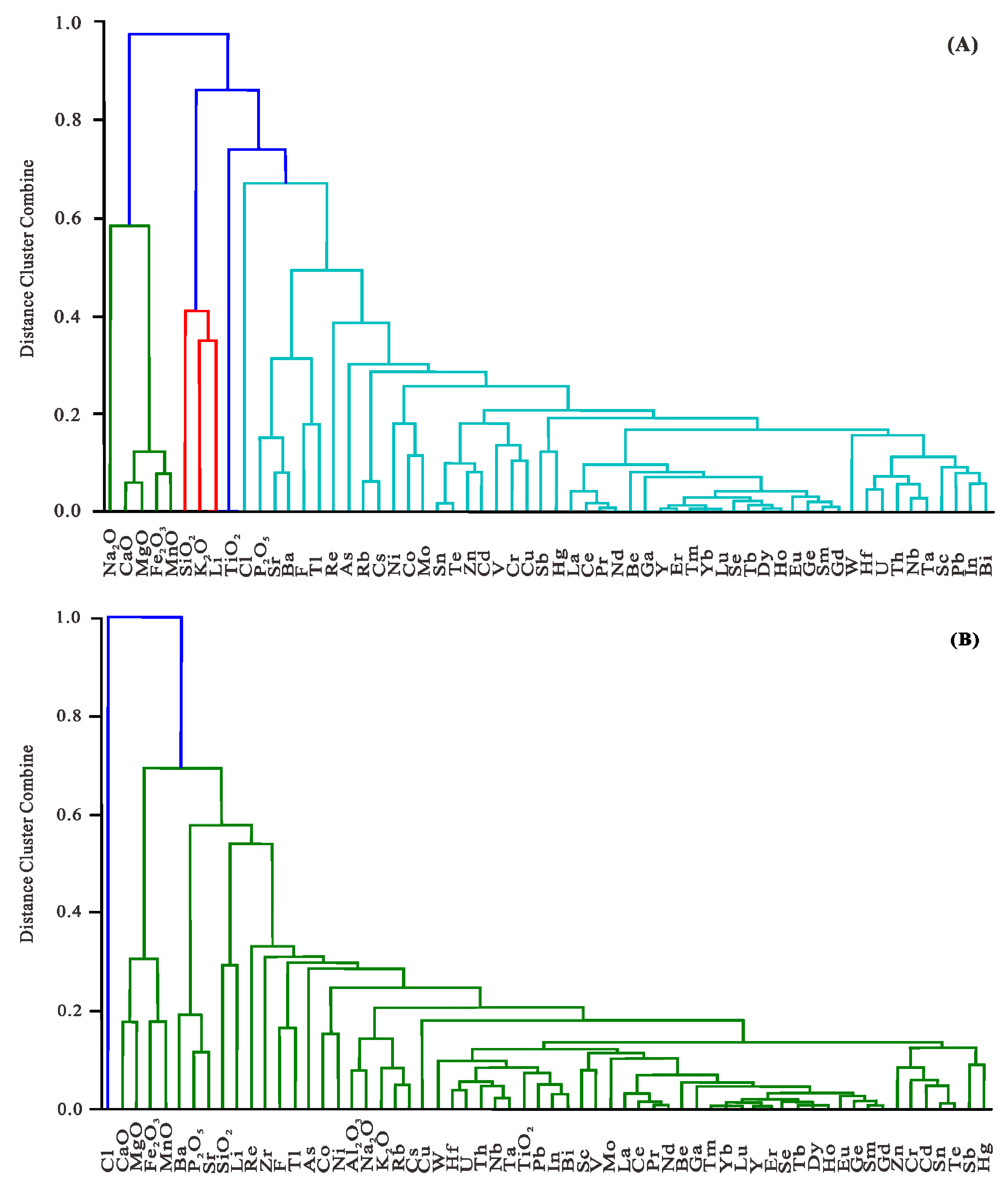
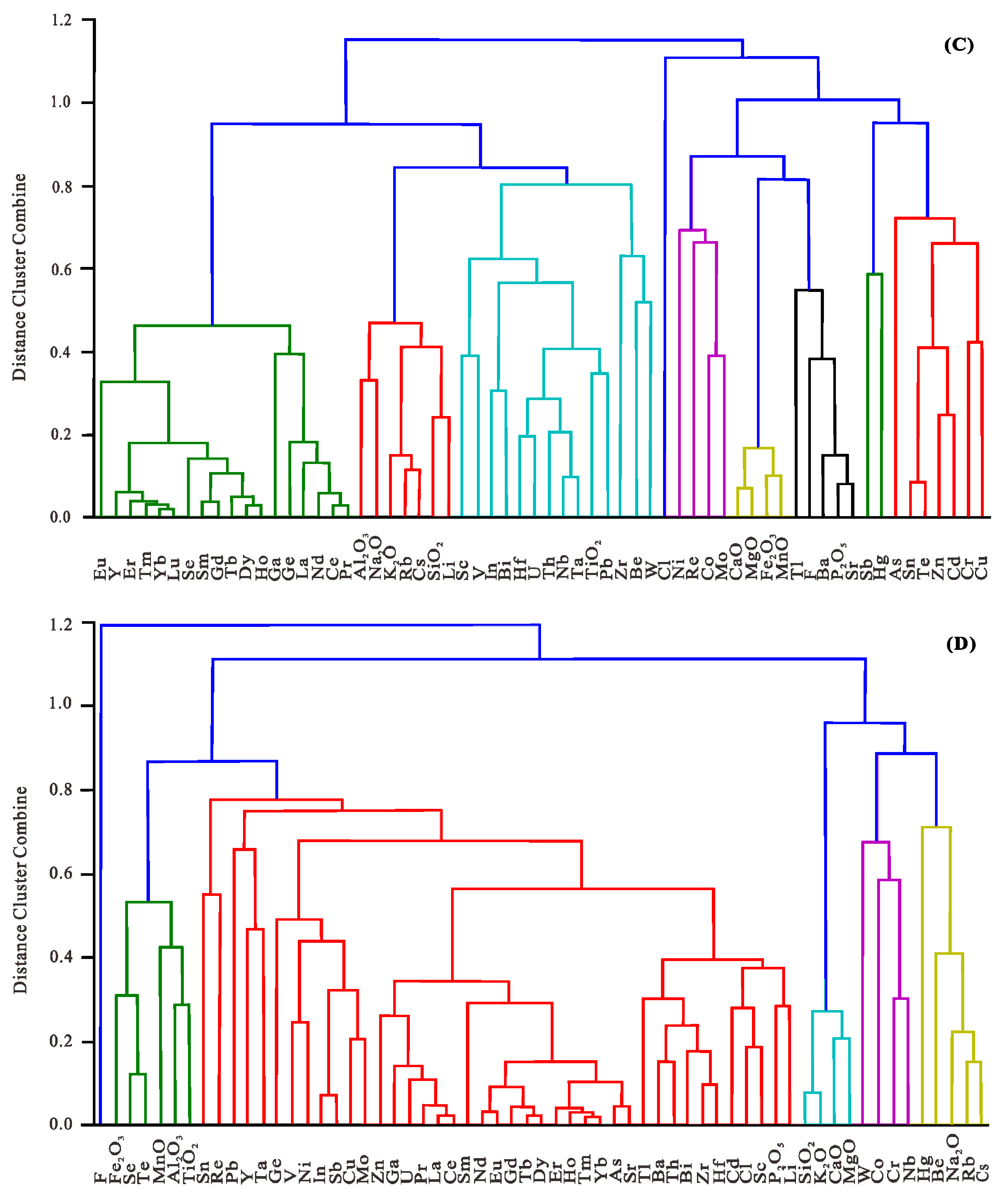
To demonstrate the consistent interpretation of whole-coal and ash bases of element concentrations, we used the data on element concentrations in the coal and ash samples from the Datanhao and Adaohai mines (Inner Mongolia, China). The coal geochemistry data are transformed based on different coal geochemistry data transformation methods: in particular, the improved alr, Geboy et al.’s method [16], clr and ilr, and the occurrence modes of elements are then deduced. All the hierarchy clustering results from different transformation methods are shown in Figure 1 and Figure 2.

As with other elements, concentrations of rare earth elements and yttrium (REY) could be reported either on ash basis or on whole-coal basis [31,32,33,34,35,36], and the ash basis is particularly suitable for REY potential recovery evaluation in coal combustion products [8,9]. In either case of basis, it would be expected that the REY should generally be clustered together if a method is effective. On the basis of trace-elements’ geochemical nature and on the investigations by Zhao et al. [15] and Dai et al. [13] using directed analysis (such as SEM-EDS, XRD), the geochemical nature of the two elements in each pair of the following elements, i.e., Sr versus Ba, Sn versus Hg, Cd versus Zn, and Nb versus Ta, is similar. Additionally, the major elements including Ca, Mg, Mn and Fe would be expected to be clustered together. Furthermore, Al and Si are both largely associated with silicate minerals and should be expected to be clustered.

The geochemistry data of the coals from the Datanhao mine were used for performance evaluation of all the methods, and the results show that our improved alr is much better predicting the modes of occurrence of the elements, as shown in Figure 1. The prediction accuracy was much better in the similarity of Cd and Zn for the improved alr than Geboy et al.’s method [16]. Note that Cd and Zn were not clustered together in Geboy et al.’s [16] method; however, as indicated by Zhao et al. [15] using the direct analysis, the Cd and Zn were both associated with sulfide minerals in these coals. On the other hand, all the rare earth elements were closeted together using the two methods, as shown in Figure 1. In addition, the similarities of the trace elements Sr and Ba, Nb and Ta were the same for the two methods (cf. Figure 1). Finally, the predictions by the two methods on the similarities of the major elements Ca, Mg, Mn and Fe were also the same according to Figure 1.

The coal geochemistry data of the Adaohai mine can also be used for performance evaluation of all the methods, and the results show that our improved alr was more appropriate in predicting occurrence modes of elements than that proposed by Geboy et al. [16]. As shown in Figure 2, the prediction accuracy was much better in the similarity of Cd and Zn for our improved alr than Geboy et al.’s [16] method. The same result also appears in Ba and Sr (that is, the improved alr is better than Geboy et al.’s method [16]). In representing the similarities among all the rare earth elements, the two methods exhibited the same results. Meanwhile, the similarities of the major elements Ca, Mg, Mn and Fe predicted are the same by using the improved alr and Geboy et al.’ s [16] method. Furthermore, the similarity of the trace elements Nb and Ta was also the same for the two methods as shown in Figure 2.

For comprehensive performance evaluation, the coal geochemistry data of the Datanhao mine was used for comparisons, and the results show that improved alr works much better in occurrence modes of element prediction than clr and ilr do, as shown in Figure 1. For the improved alr, the prediction accuracy was much better in terms of the similarity of Cd and Zn, rare earth elements, trace elements Sr and Ba, Nb and Ta, and the major elements Ca, Mg, Mn and Fe. In contrast, Cd and Zn were not clustered together by the clr method; additionally, Cd and Zn, rare earth elements, trace elements Nb and Ta, and the major elements Ca, Mg, Mn and Fe were not clustered together by the ilr method.

For comprehensive performance evaluation, the coal geochemistry data of the Adaohai mine were used for comparisons, and the results show that our improved alr works much better in occurrence modes of element prediction than clr and ilr do, as shown in Figure 2. For the improved alr, the prediction accuracy was much better in the similarity of Cd and Zn, trace elements Sr and Ba, Nb and Ta, and the major elements Ca, Mg, Mn and Fe. In contrast, the trace elements Sr and Ba were not clustered together by the clr method; additionally, Cd and Zn, trace elements Sr and Ba, Nb and Ta, and the major elements Ca, Mg, Mn and Fe were not clustered together by the ilr method.

While more meaningful geological results are produced by the proposed transformation, we acknowledge that there are still a few anomalies. For example, in the Datanhao samples, Sc-Tl, F-Ga and Hf-Pb were agglomerated very early in the clustering process. Similarly, the Adaohai samples F-Tl, Co-Mo, Hf-U, and Th-Nb were agglomerated very early. Although it is hard to think of a possible geological explanation for this relationship, some can be reasonably inferred. For example, based on selective leaching, Wang et al. [39] found that F is elevated in the similar coals in the Haerwusu coals in the Jungar coalfield, which is closely located to the south of the Daqingshan coalfield, and occurs mainly in boehmite and kaolinite. High gallium concentration is these coals is also associated with these two minerals [30,31,32,33,34,35,36,37,38,39,40,41,42]. However, other associations such as Sc-Tl and F-Tl need further investigation.

6. Conclusions

The correlation between element concentrations has been reported inconsistently for ash and whole-coal bases, which is an enduring problem well known in the research community. In this study, we show that (1) the improved alr data transformation proposed for correlations between element concentrations is consistent regardless of using different reporting bases; (2) the stability proposed by Geboy et al. [16] shows consistency between elements in coal, with similar correlations regardless of different reporting bases; (3) to verify the performance of the improved alr and Geboy et al.’s transformation methods [16] for elements in coal, a prediction model for occurrence mode of element in coal can be elegantly built using the hierarchy clustering algorithm [20]. The prediction results show that our improved alr is much better than Geboy et al.’s method [16].

In conclusion, the improved alr is much better than any of the ilr, the clr, and Geboy et al.’ s [16] approach. An interesting line of future work is to consider consistent interpretations of coal geochemistry data on whole-coal versus ash bases through deep learning [43,44,45].

Author Contributions

Conceptualization, N.X.; Methodology, N.X. and M.P.; Software, M.P. and C.X.; Validation, N.X., C.X. and M.P.; Writing—Original Draft Preparation, N.X. and Q.L.; Writing—Review & Editing, Q.L.; Supervision, N.X.; Project Administration, N.X.; Funding Acquisition, N.X. All authors have read and agreed to the published version of the manuscript.

Funding

This research was funded by the National Natural Science Foundation of China (No. 61772320) and 111 Projects (No. B17042).

Acknowledgments

We thank Robert B. Finkelman of the University of Texas at Dallas for help with the manuscript revision. Thanks are given to the editor and three anonymous reviewers for their careful reviews and detailed comments.

Conflicts of Interest

The authors declare no conflict of interest.

References

Dai, S.; Hower, J.C.; Finkelman, R.B.; Graham, I.T.; French, D.; Ward, C.R.; Eskenazy, G.; Wei, Q.; Zhao, L. Organic associations of non-mineral elements in coal: A review. Int. J. Coal Geol. 2020, 218, 103347. [Google Scholar] [CrossRef]
Finkelman, R.B.; Palmer, C.A.; Wang, P. Quantification of the modes of occurrence of 42 elements in coal. Int. J. Coal Geol. 2018, 185, 138–160. [Google Scholar] [CrossRef]
Querol, X.; Alastuey, A.; Zhuang, X.; Hower, J.; Lopez-Soler, A.; Plana, F.; Zeng, R. Petrology, mineralogy and geochemistry of the Permian and Triassic coals in the Leping area, Jiangxi Province, southeast China. Int. J. Coal Geol. 2001, 48, 23–45. [Google Scholar] [CrossRef]
Dai, S.; Ren, D.; Chou, C.-L.; Finkelman, R.B.; Seredin, V.V.; Zhou, Y. Geochemistry of trace elements in Chinese coals: A review of abundances, genetic types, impacts on human health, and industrial utilization. Int. J. Coal Geol. 2012, 94, 3–21. [Google Scholar] [CrossRef]
Swaine, D.J. Trace Elements in Coal; Butterworths: London, UK, 1990. [Google Scholar]
Ward, C. Analysis and significance of mineral matter in coal seams. Int. J. Coal Geol. 2002, 50, 135–168. [Google Scholar] [CrossRef]
Ward, C. Analysis, origin and significance of mineral matter in coal: An updated review. Int. J. Coal Geol. 2016, 165, 1–27. [Google Scholar] [CrossRef]
Dai, S.; Finkelman, R.B. Coal as a promising source of critical elements: Progress and future prospects. Int. J. Coal Geol. 2018, 186, 155–164. [Google Scholar] [CrossRef]
Dai, S.; Yan, X.; Ward, C.; Hower, J.C.; Zhao, L.; Wang, X.; Zhao, L.; Ren, D.; Finkelman, R. Valuable elements in Chinese coals: A review. Int. Geol. Rev. 2016, 60, 590–620. [Google Scholar] [CrossRef]
Seredin, V.V.; Dai, S. Coal deposits as potential alternative sources for lanthanides and yttrium. Int. J. Coal Geol. 2012, 94, 67–93. [Google Scholar] [CrossRef]
Dai, S.; Bechtel, A.; Eble, C.F.; Flores, R.M.; French, D.; Graham, I.T.; Hood, M.M.; Hower, J.C.; Korasidis, V.A.; Moore, T.A.; et al. Recognition of peat depositional environments in coal: A review. Int. J. Coal Geol. 2020, 219, 103383. [Google Scholar] [CrossRef]
Finkelman, R.B.; Dai, S.; French, D. The importance of minerals in coal as the hosts of chemical elements: A review. Int. J. Coal Geol. 2019, 212, 103251. [Google Scholar] [CrossRef]
Dai, S.; Zou, J.; Jiang, Y.; Ward, C.; Wang, X.; Li, T.; Xue, W.; Liu, S.; Tian, H.; Sun, X.; et al. Mineralogical and geochemical compositions of the Pennsylvanian coal in the Adaohai Mine, Daqingshan Coalfield, Inner Mongolia, China: Modes of occurrence and origin of diaspore, gorceixite, and ammonian illite. Int. J. Coal Geol. 2012, 94, 250–270. [Google Scholar] [CrossRef]
Xu, N.; Finkelman, R.B.; Xu, C.; Dai, S. What do coal geochemistry statistics really mean? Fuel 2020, 267, 117084. [Google Scholar] [CrossRef]
Zhao, L.; Dai, S.; Nechaev, V.P.; Nechaeva, E.V.; Graham, I.T.; French, D.; Sun, J. Enrichment of critical elements (Nb-Ta-Zr-Hf-REE) within coal and host rocks from the Datanhao mine, Daqingshan Coalfield, northern China. Ore Geol. Rev. 2019, 111, 102951. [Google Scholar] [CrossRef]
Geboy, N.; Engle, M.; Hower, J.C. Whole-coal versus ash basis in coal geochemistry: A mathematical approach to consistent interpretations. Int. J. Coal Geol. 2013, 113, 41–49. [Google Scholar] [CrossRef]
Aitchison, J. The Statistical Analysis of Compositional Data; Springer Science and Business Media LLC: Berlin/Heidelberg, Germany, 1986. [Google Scholar]
Filzmoser, P.; Hron, K.; Reimann, C. Univariate statistical analysis of environmental (compositional) data: Problems and possibilities. Sci. Total. Environ. 2009, 407, 6100–6108. [Google Scholar] [CrossRef]
Egozcue, J.J.; Pawlowsky-Glahn, V.; Mateu-Figueras, G.; Barceló-Vidal, C. Isometric Logratio Transformations for Compositional Data Analysis. Math. Geol. 2003, 35, 279–300. [Google Scholar] [CrossRef]
Xu, R.; WunschII, D. Survey of Clustering Algorithms. IEEE Trans. Neural Netw. 2005, 16, 645–678. [Google Scholar] [CrossRef] [Green Version]
Arbuzov, S.I.; Chekryzhov, I.; Finkelman, R.; Sun, Y.; Zhao, C.; Il’Enok, S.; Blokhin, M.; Zarubina, N. Comments on the geochemistry of rare-earth elements (La, Ce, Sm, Eu, Tb, Yb, Lu) with examples from coals of north Asia (Siberia, Russian far East, North China, Mongolia, and Kazakhstan). Int. J. Coal Geol. 2019, 206, 106–120. [Google Scholar] [CrossRef]
Erkoyun, H.; Kadir, S.; Huggett, J. Occurrence and genesis of tonsteins in the Miocene lignite, Tunçbilek Basin, Kütahya, western Turkey. Int. J. Coal Geol. 2019, 202, 46–68. [Google Scholar] [CrossRef]
Ribeiro, J.; Machado, G.; Moreira, N.; Suárez-Ruiz, I.; Flores, D. Petrographic and geochemical characterization of coal from Santa Susana Basin, Portugal. Int. J. Coal Geol. 2019, 203, 36–51. [Google Scholar] [CrossRef]
Wang, X.; Wang, X.; Pan, Z.; Pan, W.; Yin, X.; Chai, P.; Pan, S.; Yang, Q. Mineralogical and geochemical characteristics of the Permian coal from the Qinshui Basin, northern China, with emphasis on lithium enrichment. Int. J. Coal Geol. 2019, 214, 103254. [Google Scholar] [CrossRef]
Dai, S.; Hower, J.C.; Ward, C.; Guo, W.; Song, H.; O’Keefe, J.M.; Xie, P.; Hood, M.M.; Yan, X. Elements and phosphorus minerals in the middle Jurassic inertinite-rich coals of the Muli Coalfield on the Tibetan Plateau. Int. J. Coal Geol. 2015, 144, 23–47. [Google Scholar] [CrossRef]
Dai, S.; Ren, D.; Tang, Y.; Yue, M.; Hao, L. Concentration and distribution of elements in Late Permian coals from western Guizhou Province, China. Int. J. Coal Geol. 2005, 61, 119–137. [Google Scholar] [CrossRef]
Liu, J.; Song, H.; Dai, S.; Nechaev, V.P.; Graham, I.T.; French, D.; Nechaeva, E.V. Mineralization of REE-Y-Nb-Ta-Zr-Hf in Wuchiapingian coals from the Liupanshui Coalfield, Guizhou, southwestern China: Geochemical evidence for terrigenous input. Ore Geol. Rev. 2019, 115, 103190. [Google Scholar] [CrossRef]
Spiro, B.F.; Liu, J.; Dai, S.; Zeng, R.; Large, D.; French, D. Marine derived 87Sr/86Sr in coal, a new key to geochronology and palaeoenvironment: Elucidation of the India-Eurasia and China-Indochina collisions in Yunnan, China. Int. J. Coal Geol. 2019, 215, 103304. [Google Scholar] [CrossRef]
Dai, S.; Ward, C.; Graham, I.T.; French, D.; Hower, J.C.; Zhao, L.; Wang, X. Altered volcanic ashes in coal and coal-bearing sequences: A review of their nature and significance. Earth-Science Rev. 2017, 175, 44–74. [Google Scholar] [CrossRef]
Dai, S.; Seredin, V.V.; Ward, C.; Hower, J.C.; Xing, Y.; Zhang, W.; Song, W.; Wang, P. Enrichment of U–Se–Mo–Re–V in coals preserved within marine carbonate successions: Geochemical and mineralogical data from the Late Permian Guiding Coalfield, Guizhou, China. Miner. Deposita 2014, 50, 159–186. [Google Scholar] [CrossRef]
Chelgani, S.C. Investigating the occurrences of valuable trace elements in African coals as potential byproducts of coal and coal combustion products. J. Afr. Earth Sci. 2019, 150, 131–135. [Google Scholar] [CrossRef]
Kuppusamy, V.K.; Holuszko, M. Rare earth elements in flotation products of coals from East Kootenay coalfields, British Columbia. J. Rare Earths 2019, 37, 1366–1372. [Google Scholar] [CrossRef]
Li, B.; Zhuang, X.; Querol, X.; Li, J.; Moreno, N.; Córdoba, P.; Shangguan, Y.; Zhou, J.; Ma, X.; Liu, S. Geological controls on enrichment of Mn, Nb (Ta), Zr (Hf), and REY within the Early Permian coals of the Jimunai Depression, Xinjiang Province, NW China. Int. J. Coal Geol. 2019, 215, 103298. [Google Scholar] [CrossRef]
Medunić, G.; Grigore, M.; Dai, S.; Berti, D.; Hochella, M.F.; Mastalerz, M.; Valentim, B.; Guedes, A.; Hower, J.C. Characterization of superhigh-organic-sulfur Raša coal, Istria, Croatia, and its environmental implication. Int. J. Coal Geol. 2020, 217, 103344. [Google Scholar] [CrossRef]
Dai, S.; Wang, X.; Seredin, V.V.; Hower, J.C.; Ward, C.; O’Keefe, J.M.; Huang, W.; Li, T.; Li, X.; Liu, H.; et al. Petrology, mineralogy, and geochemistry of the Ge-rich coal from the Wulantuga Ge ore deposit, Inner Mongolia, China: New data and genetic implications. Int. J. Coal Geol. 2012, 90, 72–99. [Google Scholar] [CrossRef]
Dai, S.; Graham, I.T.; Ward, C. A review of anomalous rare earth elements and yttrium in coal. Int. J. Coal Geol. 2016, 159, 82–95. [Google Scholar] [CrossRef]
Filzmoser, P.; Hron, K.; Reimann, C. The bivariate statistical analysis of environmental (compositional) data. Sci. Total. Environ. 2010, 408, 4230–4238. [Google Scholar] [CrossRef]
Cohen-Addad, V.; Kanade, V.; Mallmann-Trenn, F.; Mathieu, C. Hierarchical Clustering: Objective Functions and Algorithms. In Proceedings of the Twenty-Ninth Annual ACM-SIAM Symposium on Discrete Algorithms; Society for Industrial & Applied Mathematics (SIAM), New Orleans, LA, USA, 7–10 January 2018; pp. 378–397. [Google Scholar]
Wang, X.; Dai, S.; Sun, Y.; Li, D.; Zhang, W.; Zhang, Y.; Luo, Y. Modes of occurrence of fluorine in the Late Paleozoic No. 6 coal from the Haerwusu Surface Mine, Inner Mongolia, China. Fuel 2011, 90, 248–254. [Google Scholar] [CrossRef]
Dai, S.; Ren, D.; Chou, C.-L.; Li, S.; Jiang, Y. Mineralogy and geochemistry of the No. 6 Coal (Pennsylvanian) in the Junger Coalfield, Ordos Basin, China. Int. J. Coal Geol. 2006, 66, 253–270. [Google Scholar] [CrossRef]
Dai, S.; Li, D.; Chou, C.-L.; Zhao, L.; Zhang, Y.; Ren, D.; Ma, Y.; Sun, Y. Mineralogy and geochemistry of boehmite-rich coals: New insights from the Haerwusu Surface Mine, Jungar Coalfield, Inner Mongolia, China. Int. J. Coal Geol. 2008, 74, 185–202. [Google Scholar] [CrossRef]
Dai, S.; Zhao, L.; Peng, S.; Chou, C.-L.; Wang, X.; Zhang, Y.; Li, D.; Sun, Y. Abundances and distribution of minerals and elements in high-alumina coal fly ash from the Jungar Power Plant, Inner Mongolia, China. Int. J. Coal Geol. 2010, 81, 320–332. [Google Scholar] [CrossRef]
Li, L.; Ota, K.; Dong, M. Deep Learning for Smart Industry: Efficient Manufacture Inspection System with Fog Computing. IEEE Trans. Ind. Inform. 2018, 14, 4665–4673. [Google Scholar] [CrossRef] [Green Version]
Chen, M.; Wang, T.; Ota, K.; Dong, M.; Zhao, M.; Liu, A. Intelligent resource allocation management for vehicles network: An A3C learning approach. Comput. Commun. 2020, 151, 485–494. [Google Scholar] [CrossRef]
Feng, B.; Fu, Q.; Dong, M.; Guo, N.; Li, Q. Multistage and Elastic Spam Detection in Mobile Social Networks through Deep Learning. IEEE Netw. 2018, 32, 15–21. [Google Scholar] [CrossRef]

Figure 1. Cluster analysis for coal element data from the Datanhao mine. (A) Improved alr on coal and ash basis; (B) Geboy’s approach on coal and ash basis; (C) clr on coal and ash basis; (D) ilr on coal and ash basis.

Figure 2. Cluster analysis for coal element data from the Adaohai mine. (A) Improved alr on coal and ash basis; (B) Geboy’s approach on coal and ash basis; (C) clr on coal and ash basis; (D) ilr on coal and ash basis.

Table 1. Stability using Geboy’s approach on coal and ash basis (Datanhao mine).

	SiO₂	TiO₂	Al₂O₃	Fe₂O₃	MgO	CaO	MnO	K₂O	P₂O₅	Li	Be	B	F	Sc	V	Cr	Co	Ni	Cu	Zn	Ga	Ge
SiO₂	1	0.890	0.964	0.310	0.346	0.213	0.206	0.835	0.828	0.419	0.803	0.551	0.940	0.804	0.647	0.669	0.481	0.572	0.734	0.606	0.932	0.734
TiO₂	0.890	1	0.875	0.297	0.316	0.206	0.206	0.670	0.817	0.451	0.805	0.470	0.834	0.828	0.696	0.675	0.470	0.555	0.774	0.544	0.903	0.714
Al₂O₃	0.964	0.875	1	0.302	0.322	0.214	0.204	0.757	0.821	0.431	0.795	0.513	0.942	0.803	0.597	0.597	0.440	0.531	0.688	0.590	0.944	0.709
Fe₂O₃	0.310	0.297	0.302	1	0.764	0.773	0.802	0.263	0.478	0.116	0.395	0.159	0.364	0.503	0.438	0.403	0.508	0.508	0.418	0.269	0.371	0.502
MgO	0.346	0.316	0.322	0.764	1	0.689	0.502	0.352	0.456	0.120	0.419	0.217	0.399	0.469	0.435	0.396	0.459	0.457	0.437	0.286	0.398	0.512
CaO	0.213	0.206	0.214	0.773	0.689	1	0.652	0.165	0.365	0.059	0.328	0.088	0.270	0.371	0.313	0.269	0.428	0.401	0.337	0.207	0.276	0.422
MnO	0.206	0.206	0.204	0.802	0.502	0.652	1	0.152	0.338	0.088	0.301	0.089	0.237	0.400	0.331	0.320	0.408	0.407	0.320	0.185	0.267	0.406
K₂O	0.835	0.670	0.757	0.263	0.352	0.165	0.152	1	0.644	0.350	0.560	0.571	0.803	0.579	0.473	0.535	0.341	0.416	0.531	0.480	0.716	0.515
P₂O₅	0.828	0.817	0.821	0.478	0.456	0.365	0.338	0.644	1	0.354	0.775	0.461	0.872	0.821	0.684	0.656	0.571	0.649	0.726	0.572	0.841	0.758
Li	0.419	0.451	0.431	0.116	0.120	0.059	0.088	0.350	0.354	1	0.385	0.223	0.389	0.376	0.299	0.425	0.162	0.271	0.324	0.213	0.449	0.294
Be	0.803	0.805	0.795	0.395	0.419	0.328	0.301	0.560	0.775	0.385	1	0.382	0.790	0.889	0.753	0.741	0.654	0.743	0.890	0.493	0.866	0.908
B	0.551	0.470	0.513	0.159	0.217	0.088	0.089	0.571	0.461	0.223	0.382	1	0.514	0.387	0.335	0.351	0.232	0.262	0.342	0.292	0.477	0.371
F	0.940	0.834	0.942	0.364	0.399	0.270	0.237	0.803	0.872	0.389	0.790	0.514	1	0.792	0.602	0.608	0.471	0.566	0.700	0.586	0.904	0.721
Sc	0.804	0.828	0.803	0.503	0.469	0.371	0.400	0.579	0.821	0.376	0.889	0.387	0.792	1	0.824	0.772	0.648	0.712	0.864	0.505	0.877	0.886
V	0.647	0.696	0.597	0.438	0.435	0.313	0.331	0.473	0.684	0.299	0.753	0.335	0.602	0.824	1	0.846	0.691	0.725	0.883	0.413	0.677	0.804
Cr	0.669	0.675	0.597	0.403	0.396	0.269	0.320	0.535	0.656	0.425	0.741	0.351	0.608	0.772	0.846	1	0.648	0.768	0.799	0.420	0.700	0.770
Co	0.481	0.470	0.440	0.508	0.459	0.428	0.408	0.341	0.571	0.162	0.654	0.232	0.471	0.648	0.691	0.648	1	0.881	0.728	0.349	0.524	0.745
Ni	0.572	0.555	0.531	0.508	0.457	0.401	0.407	0.416	0.649	0.271	0.743	0.262	0.566	0.712	0.725	0.768	0.881	1	0.767	0.373	0.617	0.776
Cu	0.734	0.774	0.688	0.418	0.437	0.337	0.320	0.531	0.726	0.324	0.890	0.342	0.700	0.864	0.883	0.799	0.728	0.767	1	0.475	0.784	0.877
Zn	0.606	0.544	0.590	0.269	0.286	0.207	0.185	0.480	0.572	0.213	0.493	0.292	0.586	0.505	0.413	0.420	0.349	0.373	0.475	1	0.593	0.485
Ga	0.932	0.903	0.944	0.371	0.398	0.276	0.267	0.716	0.841	0.449	0.866	0.477	0.904	0.877	0.677	0.700	0.524	0.617	0.784	0.593	1	0.811
Ge	0.734	0.714	0.709	0.502	0.512	0.422	0.406	0.515	0.758	0.294	0.908	0.371	0.721	0.886	0.804	0.770	0.745	0.776	0.877	0.485	0.811	1

Table 2. Correlation using the improved alr approach on coal and ash basis (Datanhao mine).

	SiO₂	TiO₂	Fe₂O₃	MgO	CaO	MnO	K₂O	P₂O₅	Li	Be	B	F	Sc	V	Cr	Co	Ni	Cu	Zn	Ga	Ge
SiO₂	1	0.386	0.150	0.270	0.074	0.099	0.668	0.263	−0.173	−0.162	0.102	−0.183	−0.217	0.253	0.398	0.192	0.154	0.204	−0.030	−0.328	−0.007
TiO₂	0.386	1	0.147	0.148	0.107	0.152	0.029	0.398	−0.020	−0.154	−0.224	−0.457	−0.094	0.286	0.172	0.017	−0.028	0.223	−0.248	−0.365	−0.173
Fe₂O₃	0.150	0.147	1	0.885	0.913	0.930	0.123	0.676	−0.295	−0.022	−0.252	−0.229	0.236	0.379	0.258	0.522	0.452	0.228	−0.061	−0.299	0.386
MgO	0.270	0.148	0.885	1	0.871	0.758	0.327	0.577	−0.333	−0.058	−0.144	−0.235	0.060	0.287	0.167	0.412	0.322	0.176	−0.082	−0.332	0.314
CaO	0.074	0.107	0.913	0.871	1	0.864	0.015	0.664	−0.429	0.059	−0.369	−0.226	0.167	0.269	0.116	0.512	0.414	0.252	−0.053	−0.296	0.431
MnO	0.099	0.152	0.930	0.758	0.864	1	−0.015	0.628	−0.253	−0.005	−0.350	−0.304	0.256	0.331	0.266	0.490	0.431	0.215	−0.099	−0.305	0.406
K₂O	0.668	0.029	0.123	0.327	0.015	−0.015	1	0.077	0.060	−0.181	0.403	0.196	−0.129	0.080	0.300	0.022	0.039	0.034	0.079	−0.012	−0.114
P₂O₅	0.263	0.398	0.676	0.577	0.664	0.628	0.077	1	−0.218	−0.047	−0.125	−0.143	0.082	0.361	0.225	0.422	0.366	0.190	−0.033	−0.312	0.216
Li	−0.173	−0.020	−0.295	−0.333	−0.429	−0.253	0.060	−0.218	1	0.207	0.138	0.282	0.176	−0.067	0.356	−0.250	0.049	−0.056	−0.003	0.395	−0.148
Be	−0.162	−0.154	−0.022	−0.058	0.059	−0.005	−0.181	−0.047	0.207	1	−0.002	0.509	0.658	0.240	0.317	0.449	0.545	0.629	0.092	0.554	0.709
B	0.102	−0.224	−0.252	−0.144	−0.369	−0.350	0.403	−0.125	0.138	−0.002	1	0.433	0.013	−0.130	0.005	−0.116	−0.117	−0.225	0.111	0.289	−0.062
F	−0.183	−0.457	−0.229	−0.235	−0.226	−0.304	0.196	−0.143	0.282	0.509	0.433	1	0.512	−0.035	0.098	0.076	0.199	0.177	0.420	0.815	0.285
Sc	−0.217	−0.094	0.236	0.060	0.167	0.256	−0.129	0.082	0.176	0.658	0.013	0.512	1	0.480	0.412	0.434	0.464	0.528	0.125	0.590	0.633
V	0.253	0.286	0.379	0.287	0.269	0.331	0.080	0.361	−0.067	0.240	−0.130	−0.035	0.480	1	0.645	0.545	0.511	0.641	−0.132	−0.119	0.396
Cr	0.398	0.172	0.258	0.167	0.116	0.266	0.300	0.225	0.356	0.317	0.005	0.098	0.412	0.645	1	0.473	0.627	0.460	−0.016	0.135	0.390
Co	0.192	0.017	0.522	0.412	0.512	0.490	0.022	0.422	−0.250	0.449	−0.116	0.076	0.434	0.545	0.473	1	0.871	0.639	0.055	0.042	0.670
Ni	0.154	−0.028	0.452	0.322	0.414	0.431	0.039	0.366	0.049	0.545	−0.117	0.199	0.464	0.511	0.627	0.871	1	0.604	0.024	0.164	0.625
Cu	0.204	0.223	0.228	0.176	0.252	0.215	0.034	0.190	−0.056	0.629	−0.225	0.177	0.528	0.641	0.460	0.639	0.604	1	−0.029	0.145	0.556
Zn	−0.030	−0.248	−0.061	−0.082	−0.053	−0.099	0.079	−0.033	−0.003	0.092	0.111	0.420	0.125	−0.132	−0.016	0.055	0.024	−0.029	1	0.366	0.046
Ga	−0.328	−0.365	−0.299	−0.332	−0.296	−0.305	−0.012	−0.312	0.395	0.554	0.289	0.815	0.590	−0.119	0.135	0.042	0.164	0.145	0.366	1	0.318
Ge	−0.007	−0.173	0.386	0.314	0.431	0.406	−0.114	0.216	−0.148	0.709	−0.062	0.285	0.633	0.396	0.390	0.670	0.625	0.556	0.046	0.318	1

Table 3. Correlation using the clr approach on coal and ash basis (Datanhao mine).

	SiO₂	TiO₂	Al₂O₃	Fe₂O₃	MgO	CaO	MnO	K₂O	P₂O₅	Li	Be	B	F	Sc	V	Cr	Co	Ni	Cu	Zn	Ga	Ge
SiO₂	1	0.625	0.891	−0.635	−0.512	−0.687	−0.649	0.737	0.241	0.325	0.041	0.486	0.786	−0.026	−0.303	−0.137	−0.495	−0.418	−0.233	0.306	0.709	−0.382
TiO₂	0.625	1	0.617	−0.593	−0.559	−0.627	−0.555	0.292	0.285	0.422	0.168	0.264	0.429	0.242	0.008	−0.021	−0.431	−0.374	0.096	0.148	0.639	−0.331
Al₂O₃	0.891	0.617	1	−0.537	−0.499	−0.551	−0.535	0.538	0.329	0.369	0.157	0.387	0.822	0.148	−0.370	−0.308	−0.529	−0.444	−0.290	0.291	0.832	−0.313
Fe₂O₃	−0.635	−0.593	−0.537	1	0.789	0.848	0.880	−0.306	0.043	−0.333	−0.393	−0.289	−0.343	0.087	0.032	−0.055	0.350	0.286	−0.199	−0.114	−0.511	0.104
MgO	−0.512	−0.559	−0.499	0.789	1	0.772	0.579	−0.046	−0.104	−0.343	−0.343	−0.095	−0.251	−0.147	−0.021	−0.122	0.220	0.124	−0.178	−0.091	−0.440	0.083
CaO	−0.687	−0.627	−0.551	0.848	0.772	1	0.773	−0.429	0.029	−0.498	−0.190	−0.435	−0.333	−0.005	−0.057	−0.205	0.375	0.268	−0.093	−0.094	−0.483	0.249
MnO	−0.649	−0.555	−0.535	0.880	0.579	0.773	1	−0.449	−0.014	−0.255	−0.251	−0.390	−0.435	0.225	0.062	0.045	0.367	0.325	−0.097	−0.136	−0.447	0.257
K₂O	0.737	0.292	0.538	−0.306	−0.046	−0.429	−0.449	1	0.123	0.247	−0.301	0.549	0.651	−0.278	−0.315	−0.052	−0.437	−0.376	−0.339	0.193	0.369	−0.542
P₂O₅	0.241	0.285	0.329	0.043	−0.104	0.029	−0.014	0.123	1	0.063	−0.282	0.193	0.475	−0.077	−0.250	−0.314	−0.199	−0.179	−0.441	0.164	0.140	−0.408
Li	0.325	0.422	0.369	−0.333	−0.343	−0.498	−0.255	0.247	0.063	1	0.178	0.142	0.230	0.121	−0.048	0.360	−0.404	−0.072	−0.065	−0.033	0.438	−0.287
Be	0.041	0.168	0.157	−0.393	−0.343	−0.190	−0.251	−0.301	−0.282	0.178	1	−0.186	0.005	0.277	0.004	0.015	0.093	0.176	0.427	−0.206	0.201	0.449
B	0.486	0.264	0.387	−0.289	−0.095	−0.435	−0.390	0.549	0.193	0.142	−0.186	1	0.383	−0.209	−0.153	−0.066	−0.292	−0.334	−0.311	0.059	0.242	−0.249
F	0.786	0.429	0.822	−0.343	−0.251	−0.333	−0.435	0.651	0.475	0.230	0.005	0.383	1	−0.060	−0.483	−0.381	−0.506	−0.408	−0.375	0.253	0.595	−0.413
Sc	−0.026	0.242	0.148	0.087	−0.147	−0.005	0.225	−0.278	−0.077	0.121	0.277	−0.209	−0.060	1	0.316	0.121	0.030	−0.018	0.220	−0.209	0.202	0.243
V	−0.303	0.008	−0.370	0.032	−0.021	−0.057	0.062	−0.315	−0.250	−0.048	0.004	−0.153	−0.483	0.316	1	0.595	0.365	0.301	0.619	−0.247	−0.383	0.249
Cr	−0.137	−0.021	−0.308	−0.055	−0.122	−0.205	0.045	−0.052	−0.314	0.360	0.015	−0.066	−0.381	0.121	0.595	1	0.268	0.448	0.333	−0.183	−0.181	0.147
Co	−0.495	−0.431	−0.529	0.350	0.220	0.375	0.367	−0.437	−0.199	−0.404	0.093	−0.292	−0.506	0.030	0.365	0.268	1	0.812	0.404	−0.175	−0.506	0.451
Ni	−0.418	−0.374	−0.444	0.286	0.124	0.268	0.325	−0.376	−0.179	−0.072	0.176	−0.334	−0.408	−0.018	0.301	0.448	0.812	1	0.317	−0.263	−0.423	0.314
Cu	−0.233	0.096	−0.290	−0.199	−0.178	−0.093	−0.097	−0.339	−0.441	−0.065	0.427	−0.311	−0.375	0.220	0.619	0.333	0.404	0.317	1	−0.214	−0.196	0.341
Zn	0.306	0.148	0.291	−0.114	−0.091	−0.094	−0.136	0.193	0.164	−0.033	−0.206	0.059	0.253	−0.209	−0.247	−0.183	−0.175	−0.263	−0.214	1	0.219	−0.253
Ga	0.709	0.639	0.832	−0.511	−0.440	−0.483	−0.447	0.369	0.140	0.438	0.201	0.242	0.595	0.202	−0.383	−0.181	−0.506	−0.423	−0.196	0.219	1	−0.180
Ge	−0.382	−0.331	−0.313	0.104	0.083	0.249	0.257	−0.542	−0.408	−0.287	0.449	−0.249	−0.413	0.243	0.249	0.147	0.451	0.314	0.341	−0.253	−0.180	1

Table 4. Correlation using the ilr approach on coal and ash basis (Datanhao mine).

	SiO₂	TiO₂	Al₂O₃	Fe₂O₃	MgO	CaO	MnO	K₂O	P₂O₅	Li	Be	B	F	Sc	V	Cr	Co	Ni	Cu	Zn	Ga	Ge
SiO₂	1	−0.598	−0.014	−0.104	0.019	0.073	−0.344	0.171	0.173	0.143	−0.188	−0.271	0.366	0.333	0.143	0.035	0.022	0.337	−0.147	0.016	0.036	−0.222
TiO₂	−0.598	1	−0.030	−0.088	0.047	−0.031	0.029	−0.021	−0.019	−0.056	0.018	0.336	−0.135	−0.473	−0.478	−0.219	−0.186	−0.400	0.134	0.294	−0.030	0.217
Al₂O₃	−0.014	−0.030	1	0.795	0.834	0.783	−0.737	−0.633	−0.545	−0.553	−0.480	−0.754	−0.197	−0.034	−0.111	0.323	0.227	−0.285	−0.266	−0.768	0.028	0.257
Fe₂O₃	−0.104	−0.088	0.795	1	0.715	0.408	−0.464	−0.688	−0.519	−0.462	−0.271	−0.642	−0.380	−0.069	−0.157	0.207	0.084	−0.221	−0.222	−0.654	0.042	0.047
MgO	0.019	0.047	0.834	0.715	1	0.644	−0.795	−0.509	−0.638	−0.307	−0.592	−0.578	−0.125	−0.060	−0.192	0.381	0.264	−0.107	−0.183	−0.598	0.221	0.248
CaO	0.073	−0.031	0.783	0.408	0.644	1	−0.738	−0.485	−0.315	−0.374	−0.509	−0.702	0.073	0.030	0.057	0.299	0.261	−0.173	−0.248	−0.577	0.147	0.226
MnO	−0.344	0.029	−0.737	−0.464	−0.795	−0.738	1	0.351	0.419	0.105	0.603	0.649	−0.222	−0.155	0.069	−0.411	−0.324	−0.036	0.209	0.470	−0.358	−0.218
K₂O	0.171	−0.021	−0.633	−0.688	−0.509	−0.485	0.351	1	0.360	0.301	0.342	0.567	0.082	0.048	0.017	−0.157	−0.081	0.075	0.191	0.395	−0.123	−0.041
P₂O₅	0.173	−0.019	−0.545	−0.519	−0.638	−0.315	0.419	0.360	1	0.247	0.169	0.213	0.083	0.008	0.354	−0.386	−0.072	0.049	−0.032	0.410	−0.214	−0.300
Li	0.143	−0.056	−0.553	−0.462	−0.307	−0.374	0.105	0.301	0.247	1	0.083	0.324	0.540	0.354	0.299	0.257	0.304	0.672	−0.036	0.365	0.584	−0.054
Be	−0.188	0.018	−0.480	−0.271	−0.592	−0.509	0.603	0.342	0.169	0.083	1	0.305	−0.244	−0.098	−0.052	−0.263	−0.327	−0.144	0.074	0.242	−0.153	−0.123
B	−0.271	0.336	−0.754	−0.642	−0.578	−0.702	0.649	0.567	0.213	0.324	0.305	1	0.006	−0.224	−0.219	−0.337	−0.263	0.063	0.313	0.636	−0.135	−0.048
F	0.366	−0.135	−0.197	−0.380	−0.125	0.073	−0.222	0.082	0.083	0.540	−0.244	0.006	1	0.565	0.338	0.247	0.177	0.553	−0.142	0.189	0.460	0.103
Sc	0.333	−0.473	−0.034	−0.069	−0.060	0.030	−0.155	0.048	0.008	0.354	−0.098	−0.224	0.565	1	0.669	0.450	0.387	0.673	−0.181	−0.263	0.359	0.100
V	0.143	−0.478	−0.111	−0.157	−0.192	0.057	0.069	0.017	0.354	0.299	−0.052	−0.219	0.338	0.669	1	0.339	0.494	0.406	−0.153	−0.158	0.223	0.036
Cr	0.035	−0.219	0.323	0.207	0.381	0.299	−0.411	−0.157	−0.386	0.257	−0.263	−0.337	0.247	0.450	0.339	1	0.812	0.389	−0.162	−0.458	0.430	0.367
Co	0.022	−0.186	0.227	0.084	0.264	0.261	−0.324	−0.081	−0.072	0.304	−0.327	−0.263	0.177	0.387	0.494	0.812	1	0.313	−0.250	−0.390	0.307	0.270
Ni	0.337	−0.400	−0.285	−0.221	−0.107	−0.173	−0.036	0.075	0.049	0.672	−0.144	0.063	0.553	0.673	0.406	0.389	0.313	1	−0.047	0.075	0.460	0.006
Cu	−0.147	0.134	−0.266	−0.222	−0.183	−0.248	0.209	0.191	−0.032	−0.036	0.074	0.313	−0.142	−0.181	−0.153	−0.162	−0.250	−0.047	1	0.237	−0.198	−0.063
Zn	0.016	0.294	−0.768	−0.654	−0.598	−0.577	0.470	0.395	0.410	0.365	0.242	0.636	0.189	−0.263	−0.158	−0.458	−0.390	0.075	0.237	1	0.020	−0.207
Ga	0.036	−0.030	0.028	0.042	0.221	0.147	−0.358	−0.123	−0.214	0.584	−0.153	−0.135	0.460	0.359	0.223	0.430	0.307	0.460	−0.198	0.020	1	−0.047
Ge	−0.222	0.217	0.257	0.047	0.248	0.226	−0.218	−0.041	−0.300	−0.054	−0.123	−0.048	0.103	0.100	0.036	0.367	0.270	0.006	−0.063	−0.207	−0.047	1

Table 5. Stability using Geboy’s approach on coal and ash basis (Adaohai mine).

	Al₂O₃	SiO₂	CaO	Fe₂O₃	K₂O	MgO	MnO	Na₂O	P₂O₅	TiO₂	Li	Be	F	Sc	V	Cr	Co	Ni	Cu	Zn	Ga	Ge
Al₂O₃	1	0.614	0.258	0.411	0.817	0.187	0.284	0.924	0.422	0.866	0.515	0.908	0.820	0.806	0.811	0.854	0.709	0.752	0.713	0.746	0.922	0.842
SiO₂	0.614	1	0.097	0.159	0.729	0.060	0.099	0.693	0.117	0.581	0.708	0.503	0.342	0.543	0.512	0.461	0.352	0.416	0.389	0.348	0.565	0.514
CaO	0.258	0.097	1	0.724	0.174	0.825	0.681	0.324	0.181	0.221	0.095	0.289	0.341	0.261	0.286	0.395	0.424	0.387	0.333	0.355	0.292	0.295
Fe₂O₃	0.411	0.159	0.724	1	0.272	0.739	0.823	0.469	0.204	0.387	0.172	0.448	0.458	0.409	0.434	0.565	0.480	0.547	0.469	0.451	0.434	0.435
K₂O	0.817	0.729	0.174	0.272	1	0.119	0.182	0.794	0.307	0.804	0.622	0.752	0.620	0.726	0.661	0.676	0.534	0.585	0.546	0.571	0.772	0.694
MgO	0.187	0.060	0.825	0.739	0.119	1	0.634	0.238	0.145	0.165	0.063	0.205	0.247	0.182	0.194	0.289	0.287	0.293	0.235	0.228	0.201	0.199
MnO	0.284	0.099	0.681	0.823	0.182	0.634	1	0.328	0.151	0.248	0.111	0.320	0.367	0.266	0.291	0.408	0.318	0.349	0.333	0.363	0.307	0.318
Na₂O	0.924	0.693	0.324	0.469	0.794	0.238	0.328	1	0.353	0.785	0.606	0.824	0.739	0.754	0.765	0.837	0.706	0.779	0.684	0.705	0.859	0.794
P₂O₅	0.422	0.117	0.181	0.204	0.307	0.145	0.151	0.353	1	0.320	0.126	0.414	0.590	0.326	0.313	0.388	0.454	0.396	0.300	0.422	0.413	0.381
TiO₂	0.866	0.581	0.221	0.387	0.804	0.165	0.248	0.785	0.320	1	0.513	0.894	0.695	0.907	0.884	0.862	0.668	0.736	0.776	0.718	0.891	0.853
Li	0.515	0.708	0.095	0.172	0.622	0.063	0.111	0.606	0.126	0.513	1	0.410	0.351	0.425	0.464	0.450	0.352	0.402	0.381	0.363	0.476	0.436
Be	0.908	0.503	0.289	0.448	0.752	0.205	0.320	0.824	0.414	0.894	0.410	1	0.785	0.890	0.850	0.916	0.734	0.791	0.816	0.830	0.952	0.924
F	0.820	0.342	0.341	0.458	0.620	0.247	0.367	0.739	0.590	0.695	0.351	0.785	1	0.623	0.650	0.784	0.703	0.689	0.626	0.781	0.758	0.728
Sc	0.806	0.543	0.261	0.409	0.726	0.182	0.266	0.754	0.326	0.907	0.425	0.890	0.623	1	0.923	0.860	0.728	0.765	0.820	0.696	0.915	0.886
V	0.811	0.512	0.286	0.434	0.661	0.194	0.291	0.765	0.313	0.884	0.464	0.850	0.650	0.923	1	0.913	0.778	0.795	0.875	0.780	0.922	0.896
Cr	0.854	0.461	0.395	0.565	0.676	0.289	0.408	0.837	0.388	0.862	0.450	0.916	0.784	0.860	0.913	1	0.819	0.872	0.899	0.891	0.922	0.910
Co	0.709	0.352	0.424	0.480	0.534	0.287	0.318	0.706	0.454	0.668	0.352	0.734	0.703	0.728	0.778	0.819	1	0.847	0.770	0.757	0.776	0.725
Ni	0.752	0.416	0.387	0.547	0.585	0.293	0.349	0.779	0.396	0.736	0.402	0.791	0.689	0.765	0.795	0.872	0.847	1	0.780	0.748	0.810	0.798
Cu	0.713	0.389	0.333	0.469	0.546	0.235	0.333	0.684	0.300	0.776	0.381	0.816	0.626	0.820	0.875	0.899	0.770	0.780	1	0.831	0.832	0.844
Zn	0.746	0.348	0.355	0.451	0.571	0.228	0.363	0.705	0.422	0.718	0.363	0.830	0.781	0.696	0.780	0.891	0.757	0.748	0.831	1	0.824	0.842
Ga	0.922	0.565	0.292	0.434	0.772	0.201	0.307	0.859	0.413	0.891	0.476	0.952	0.758	0.915	0.922	0.922	0.776	0.810	0.832	0.824	1	0.964
Ge	0.842	0.514	0.295	0.435	0.694	0.199	0.318	0.794	0.381	0.853	0.436	0.924	0.728	0.886	0.896	0.910	0.725	0.798	0.844	0.842	0.964	1

Table 6. Correlation using the impoved alr on coal and ash basis (Adaohai mine).

	SiO₂	CaO	Fe₂O₃	K₂O	MgO	MnO	Na₂O	P₂O₅	TiO₂	Li	Be	F	Sc	V	Cr	Co	Ni	Cu	Zn	Ga	Ge	As
SiO₂	1	−0.301	−0.349	0.595	−0.364	−0.360	0.508	−0.613	0.167	0.587	−0.210	−0.471	0.043	−0.027	−0.237	−0.258	−0.159	−0.172	−0.376	−0.069	−0.069	−0.411
CaO	−0.301	1	0.875	−0.182	0.942	0.854	0.471	0.235	−0.011	−0.242	0.020	0.186	0.024	0.088	0.311	0.383	0.308	0.247	0.293	0.015	0.086	0.127
Fe₂O₃	−0.349	0.875	1	−0.247	0.927	0.923	0.398	0.094	0.115	−0.208	0.031	0.122	0.046	0.096	0.315	0.250	0.316	0.238	0.198	−0.017	0.069	0.156
K₂O	0.595	−0.182	−0.247	1	−0.217	−0.242	0.198	−0.139	0.374	0.653	0.346	0.119	0.404	0.262	0.239	0.102	0.158	0.133	0.148	0.347	0.298	0.201
MgO	−0.364	0.942	0.927	−0.217	1	0.853	0.435	0.253	0.017	−0.244	0.027	0.188	0.022	0.061	0.314	0.327	0.321	0.227	0.211	0.001	0.055	0.151
MnO	−0.360	0.854	0.923	−0.242	0.853	1	0.356	0.112	0.011	−0.217	0.035	0.187	−0.015	0.044	0.282	0.172	0.201	0.203	0.261	−0.011	0.085	0.148
Na₂O	0.508	0.471	0.398	0.198	0.435	0.356	1	−0.185	−0.087	0.260	−0.420	−0.349	−0.247	−0.242	−0.152	−0.078	0.020	−0.172	−0.239	−0.313	−0.255	−0.452
P₂O₅	−0.613	0.235	0.094	−0.139	0.253	0.112	−0.185	1	−0.186	−0.200	0.287	0.593	0.127	0.098	0.274	0.453	0.325	0.152	0.428	0.254	0.249	0.351
TiO₂	0.167	−0.011	0.115	0.374	0.017	0.011	−0.087	−0.186	1	0.173	0.276	−0.082	0.472	0.449	0.324	0.116	0.195	0.389	0.184	0.215	0.307	0.365
Li	0.587	−0.242	−0.208	0.653	−0.244	−0.217	0.260	−0.200	0.173	1	0.240	0.202	0.362	0.408	0.344	0.254	0.332	0.295	0.194	0.404	0.338	0.082
Be	−0.210	0.020	0.031	0.346	0.027	0.035	−0.420	0.287	0.276	0.240	1	0.684	0.869	0.765	0.848	0.656	0.723	0.773	0.730	0.918	0.880	0.771
F	−0.471	0.186	0.122	0.119	0.188	0.187	−0.349	0.593	−0.082	0.202	0.684	1	0.477	0.483	0.686	0.644	0.604	0.508	0.706	0.644	0.606	0.591
Sc	0.043	0.024	0.046	0.404	0.022	−0.015	−0.247	0.127	0.472	0.362	0.869	0.477	1	0.909	0.820	0.684	0.719	0.794	0.575	0.902	0.858	0.641
V	−0.027	0.088	0.096	0.262	0.061	0.044	−0.242	0.098	0.449	0.408	0.765	0.483	0.909	1	0.874	0.739	0.744	0.857	0.679	0.889	0.852	0.613
Cr	−0.237	0.311	0.315	0.239	0.314	0.282	−0.152	0.274	0.324	0.344	0.848	0.686	0.820	0.874	1	0.794	0.853	0.897	0.840	0.865	0.857	0.751
Co	−0.258	0.383	0.250	0.102	0.327	0.172	−0.078	0.453	0.116	0.254	0.656	0.644	0.684	0.739	0.794	1	0.840	0.750	0.710	0.729	0.652	0.513
Ni	−0.159	0.308	0.316	0.158	0.321	0.201	0.020	0.325	0.195	0.332	0.723	0.604	0.719	0.744	0.853	0.840	1	0.751	0.676	0.758	0.743	0.572
Cu	−0.172	0.247	0.238	0.133	0.227	0.203	−0.172	0.152	0.389	0.295	0.773	0.508	0.794	0.857	0.897	0.750	0.751	1	0.799	0.796	0.814	0.678
Zn	−0.376	0.293	0.198	0.148	0.211	0.261	−0.239	0.428	0.184	0.194	0.730	0.706	0.575	0.679	0.840	0.710	0.676	0.799	1	0.727	0.768	0.735
Ga	−0.069	0.015	−0.017	0.347	0.001	−0.011	−0.313	0.254	0.215	0.404	0.918	0.644	0.902	0.889	0.865	0.729	0.758	0.796	0.727	1	0.946	0.653
Ge	−0.069	0.086	0.069	0.298	0.055	0.085	−0.255	0.249	0.307	0.338	0.880	0.606	0.858	0.852	0.857	0.652	0.743	0.814	0.768	0.946	1	0.685
As	−0.411	0.127	0.156	0.201	0.151	0.148	−0.452	0.351	0.365	0.082	0.771	0.591	0.641	0.613	0.751	0.513	0.572	0.678	0.735	0.653	0.685	1

Table 7. Correlation using the clr on coal and ash basis (Adaohai mine).

	Al₂O₃	SiO₂	CaO	Fe₂O₃	K₂O	MgO	MnO	Na₂O	P₂O₅	TiO₂	Li	Be	F	Cl	Sc	V	Cr	Co	Ni	Cu	Zn	Ga
Al₂O₃	1	0.544	−0.434	−0.289	0.519	−0.341	−0.310	0.672	0.063	0.326	0.355	0.342	0.335	−0.213	−0.060	−0.049	−0.182	−0.212	−0.172	−0.325	−0.246	0.439
SiO₂	0.544	1	−0.417	−0.399	0.732	−0.437	−0.419	0.724	−0.464	0.433	0.760	0.070	−0.299	0.013	0.307	0.192	−0.220	−0.267	−0.102	−0.181	−0.415	0.448
CaO	−0.434	−0.417	1	0.820	−0.470	0.927	0.803	−0.003	0.043	−0.609	−0.349	−0.519	0.117	−0.087	−0.395	−0.256	0.245	0.368	0.240	0.059	0.121	−0.611
Fe₂O₃	−0.289	−0.399	0.820	1	−0.455	0.903	0.898	0.042	−0.100	−0.354	−0.255	−0.351	0.079	−0.156	−0.278	−0.172	0.360	0.140	0.306	0.072	−0.024	−0.568
K₂O	0.519	0.732	−0.470	−0.455	1	−0.436	−0.449	0.464	−0.115	0.480	0.612	0.146	−0.027	0.047	0.172	−0.118	−0.401	−0.368	−0.294	−0.414	−0.387	0.249
MgO	−0.341	−0.437	0.927	0.903	−0.436	1	0.812	0.035	0.097	−0.460	−0.339	−0.453	0.121	−0.195	−0.361	−0.281	0.285	0.269	0.281	0.045	−0.013	−0.605
MnO	−0.310	−0.419	0.803	0.898	−0.449	0.812	1	−0.010	−0.068	−0.467	−0.273	−0.321	0.182	−0.057	−0.394	−0.260	0.287	0.013	0.082	0.034	0.129	−0.523
Na₂O	0.672	0.724	−0.003	0.042	0.464	0.035	−0.010	1	−0.154	0.040	0.612	−0.096	0.080	−0.144	−0.171	−0.123	−0.022	−0.076	0.116	−0.286	−0.275	0.123
P₂O₅	0.063	−0.464	0.043	−0.100	−0.115	0.097	−0.068	−0.154	1	−0.370	−0.328	−0.109	0.592	−0.048	−0.373	−0.457	−0.314	0.254	0.028	−0.343	0.113	−0.171
TiO₂	0.326	0.433	−0.609	−0.354	0.480	−0.460	−0.467	0.040	−0.370	1	0.349	0.320	−0.199	0.009	0.552	0.427	0.019	−0.352	−0.182	0.069	−0.320	0.248
Li	0.355	0.760	−0.349	−0.255	0.612	−0.339	−0.273	0.612	−0.328	0.349	1	−0.251	−0.124	0.185	0.016	0.170	−0.008	−0.128	−0.010	−0.069	−0.182	0.155
Be	0.342	0.070	−0.519	−0.351	0.146	−0.453	−0.321	−0.096	−0.109	0.320	−0.251	1	−0.046	−0.267	0.226	−0.146	−0.110	−0.446	−0.306	−0.015	−0.047	0.333
F	0.335	−0.299	0.117	0.079	−0.027	0.121	0.182	0.080	0.592	−0.199	−0.124	−0.046	1	−0.005	−0.628	−0.495	−0.091	0.068	−0.107	−0.339	0.252	−0.353
Cl	−0.213	0.013	−0.087	−0.156	0.047	−0.195	−0.057	−0.144	−0.048	0.009	0.185	−0.267	−0.005	1	0.037	0.001	−0.275	0.129	0.131	−0.081	−0.066	−0.128
Sc	−0.060	0.307	−0.395	−0.278	0.172	−0.361	−0.394	−0.171	−0.373	0.552	0.016	0.226	−0.628	0.037	1	0.611	−0.072	−0.093	−0.075	0.249	−0.503	0.409
V	−0.049	0.192	−0.256	−0.172	−0.118	−0.281	−0.260	−0.123	−0.457	0.427	0.170	−0.146	−0.495	0.001	0.611	1	0.384	0.138	0.070	0.498	−0.042	0.456
Cr	−0.182	−0.220	0.245	0.360	−0.401	0.285	0.287	−0.022	−0.314	0.019	−0.008	−0.110	−0.091	−0.275	−0.072	0.384	1	0.145	0.308	0.578	0.415	−0.207
Co	−0.212	−0.267	0.368	0.140	−0.368	0.269	0.013	−0.076	0.254	−0.352	−0.128	−0.446	0.068	0.129	−0.093	0.138	0.145	1	0.505	0.245	0.145	−0.232
Ni	−0.172	−0.102	0.240	0.306	−0.294	0.281	0.082	0.116	0.028	−0.182	−0.010	−0.306	−0.107	0.131	−0.075	0.070	0.308	0.505	1	0.182	−0.027	−0.258
Cu	−0.325	−0.181	0.059	0.072	−0.414	0.045	0.034	−0.286	−0.343	0.069	−0.069	−0.015	−0.339	−0.081	0.249	0.498	0.578	0.245	0.182	1	0.373	0.032
Zn	−0.246	−0.415	0.121	−0.024	−0.387	−0.013	0.129	−0.275	0.113	−0.320	−0.182	−0.047	0.252	−0.066	−0.503	−0.042	0.415	0.145	−0.027	0.373	1	−0.200
Ga	0.439	0.448	−0.611	−0.568	0.249	−0.605	−0.523	0.123	−0.171	0.248	0.155	0.333	−0.353	−0.128	0.409	0.456	−0.207	−0.232	−0.258	0.032	−0.200	1

Table 8. Correlation using the ilr on coal and ash basis (Adaohai mine).

	Al₂O₃	SiO₂	CaO	Fe₂O₃	K₂O	MgO	MnO	Na₂O	P₂O₅	TiO₂	Li	Be	F	Cl	Sc	V	Cr	Co	Ni	Cu	Zn	Ga
Al₂O₃	1	−0.533	−0.599	0.395	−0.530	−0.502	0.468	−0.493	0.290	0.715	−0.089	−0.521	0.108	0.199	0.102	−0.212	−0.274	−0.103	−0.100	−0.351	0.146	0.116
SiO₂	−0.533	1	0.765	−0.810	0.924	0.696	−0.893	−0.109	−0.771	−0.722	−0.537	−0.135	−0.086	−0.452	−0.357	−0.074	0.203	0.023	−0.053	0.029	−0.617	−0.414
CaO	−0.599	0.765	1	−0.743	0.824	0.795	−0.835	−0.200	−0.532	−0.611	−0.399	−0.163	−0.142	−0.310	−0.246	0.031	−0.034	0.116	−0.003	−0.060	−0.521	−0.323
Fe₂O₃	0.395	−0.810	−0.743	1	−0.808	−0.685	0.681	0.310	0.688	0.589	0.486	0.235	0.177	0.340	0.149	−0.055	−0.202	−0.178	−0.075	0.016	0.465	0.262
K₂O	−0.530	0.924	0.824	−0.808	1	0.637	−0.858	−0.112	−0.749	−0.714	−0.599	−0.215	−0.227	−0.438	−0.372	−0.059	0.126	0.074	−0.071	−0.106	−0.589	−0.431
MgO	−0.502	0.696	0.795	−0.685	0.637	1	−0.759	−0.227	−0.583	−0.532	−0.352	−0.035	−0.007	−0.436	−0.326	−0.072	−0.219	−0.195	−0.048	0.091	−0.460	−0.231
MnO	0.468	−0.893	−0.835	0.681	−0.858	−0.759	1	0.255	0.593	0.686	0.470	0.225	0.084	0.315	0.299	0.108	0.020	0.108	0.035	0.084	0.540	0.336
Na₂O	−0.493	−0.109	−0.200	0.310	−0.112	−0.227	0.255	1	0.078	−0.159	0.299	0.669	0.057	0.023	−0.042	0.009	0.330	0.111	−0.083	0.268	0.202	0.120
P₂O₅	0.290	−0.771	−0.532	0.688	−0.749	−0.583	0.593	0.078	1	0.501	0.716	0.163	0.184	0.679	0.612	0.313	−0.043	0.060	0.359	0.133	0.556	0.473
TiO₂	0.715	−0.722	−0.611	0.589	−0.714	−0.532	0.686	−0.159	0.501	1	0.046	−0.116	0.247	0.079	0.168	−0.086	−0.189	−0.103	−0.014	−0.113	0.157	0.072
Li	−0.089	−0.537	−0.399	0.486	−0.599	−0.352	0.470	0.299	0.716	0.046	1	0.360	0.052	0.672	0.522	0.482	0.122	0.176	0.461	0.438	0.716	0.666
Be	−0.521	−0.135	−0.163	0.235	−0.215	−0.035	0.225	0.669	0.163	−0.116	0.360	1	0.110	−0.151	−0.082	0.068	0.138	−0.075	−0.059	0.410	0.090	0.097
F	0.108	−0.086	−0.142	0.177	−0.227	−0.007	0.084	0.057	0.184	0.247	0.052	0.110	1	−0.227	−0.258	−0.556	−0.136	−0.174	−0.271	−0.264	−0.345	−0.281
Cl	0.199	−0.452	−0.310	0.340	−0.438	−0.436	0.315	0.023	0.679	0.079	0.672	−0.151	−0.227	1	0.817	0.546	0.220	0.242	0.581	0.129	0.729	0.654
Sc	0.102	−0.357	−0.246	0.149	−0.372	−0.326	0.299	−0.042	0.612	0.168	0.522	−0.082	−0.258	0.817	1	0.721	0.354	0.312	0.697	0.358	0.684	0.628
V	−0.212	−0.074	0.031	−0.055	−0.059	−0.072	0.108	0.009	0.313	−0.086	0.482	0.068	−0.556	0.546	0.721	1	0.353	0.452	0.755	0.662	0.506	0.562
Cr	−0.274	0.203	−0.034	−0.202	0.126	−0.219	0.020	0.330	−0.043	−0.189	0.122	0.138	−0.136	0.220	0.354	0.353	1	0.500	0.362	0.278	0.088	−0.010
Co	−0.103	0.023	0.116	−0.178	0.074	−0.195	0.108	0.111	0.060	−0.103	0.176	−0.075	−0.174	0.242	0.312	0.452	0.500	1	0.318	0.150	0.106	0.194
Ni	−0.100	−0.053	−0.003	−0.075	−0.071	−0.048	0.035	−0.083	0.359	−0.014	0.461	−0.059	−0.271	0.581	0.697	0.755	0.362	0.318	1	0.544	0.402	0.507
Cu	−0.351	0.029	−0.060	0.016	−0.106	0.091	0.084	0.268	0.133	−0.113	0.438	0.410	−0.264	0.129	0.358	0.662	0.278	0.150	0.544	1	0.329	0.468
Zn	0.146	−0.617	−0.521	0.465	−0.589	−0.460	0.540	0.202	0.556	0.157	0.716	0.090	−0.345	0.729	0.684	0.506	0.088	0.106	0.402	0.329	1	0.844
Ga	0.116	−0.414	−0.323	0.262	−0.431	−0.231	0.336	0.120	0.473	0.072	0.666	0.097	−0.281	0.654	0.628	0.562	−0.010	0.194	0.507	0.468	0.844	1

Table 9. Average-linkage algorithm for hierarchical clustering.

Input: The similarities graph

G (V, E, ω) = G (V (x_{i}), E (x_{i,} x_{j}), d_{k} (x_{i,} x_{j})), e l e m e n t s n u m b e r n

.
Output: Print hierarchy clustering records.
Begin:

Initialize:

Elements clusters

C = {c_{1}, c_{2}, …, c_{n}} = {{x_{1}}, {x_{2}}, …, {x_{n}}}

,

Minimum distance

d_{m i n},

Cluster index

a, b

.

While

l e n g t h (C) > 1

do

d_{m i n} = Infinity

.

For

i = 1 \to (l e n g t h (C) - 1

) do

For

j = (i + 1) \to l e n g t h (C)

do

Calculate the distance between

c_{i}

and

c_{j}

:

d = \sum_{x_{p} \in C_{i}, x_{q} \in C_{j}} \frac{d_{k} (x_{p,} x_{q})}{| C_{i} | | C_{j} |}

If

d < d_{m i n}

then

d_{m i n} = d, a = i, b = j

.

End for

Merge cluster

c_{a}

and

c_{b}

:

c_{t m p} = c_{a} \cup c_{b}

.Delete

c_{a}

and

c_{b}

from

C

. Append

c_{t m p}

to

C .

Print elements

{V (x_{i}) | x_{i} \in c_{t m p}}

.

End While
End

© 2020 by the authors. Licensee MDPI, Basel, Switzerland. This article is an open access article distributed under the terms and conditions of the Creative Commons Attribution (CC BY) license (http://creativecommons.org/licenses/by/4.0/).

Share and Cite

MDPI and ACS Style

Xu, N.; Peng, M.; Li, Q.; Xu, C. Towards Consistent Interpretations of Coal Geochemistry Data on Whole-Coal versus Ash Bases through Machine Learning. Minerals 2020, 10, 328. https://doi.org/10.3390/min10040328

AMA Style

Xu N, Peng M, Li Q, Xu C. Towards Consistent Interpretations of Coal Geochemistry Data on Whole-Coal versus Ash Bases through Machine Learning. Minerals. 2020; 10(4):328. https://doi.org/10.3390/min10040328

Chicago/Turabian Style

Xu, Na, Mengmeng Peng, Qing Li, and Chuanpeng Xu. 2020. "Towards Consistent Interpretations of Coal Geochemistry Data on Whole-Coal versus Ash Bases through Machine Learning" Minerals 10, no. 4: 328. https://doi.org/10.3390/min10040328

Note that from the first issue of 2016, this journal uses article numbers instead of page numbers. See further details here.

Article Menu

Towards Consistent Interpretations of Coal Geochemistry Data on Whole-Coal versus Ash Bases through Machine Learning

Abstract

1. Introduction

2. Compositional Data Transformation

2.1. Additive Log-Ratio (alr) Transformation

2.2. Centered Log-Ratio (clr) Transformation

2.3. Isometric Log-Ratio (ilr) Transformation

3. Improved Additive Log-Ratio and Correlation Analysis

3.1. Improved Additive Log-Ratio Transformation

3.2. Correlation Analysis of Different Transformation Methods

3.3. Correlation Replaced by Stability

4. Prediction for Occurrence Mode of Element in Coal Based on Hierarchy Clustering

4.1. Hierarchical Clustering

4.2. Similarities Analysis between the Elements in Coal

4.3. Agglomerative Clustering Algorithm for Prediction

5. Results

6. Conclusions

Author Contributions

Funding

Acknowledgments

Conflicts of Interest

References

Share and Cite

Article Metrics

Article Access Statistics

Further Information

Guidelines

MDPI Initiatives

Follow MDPI