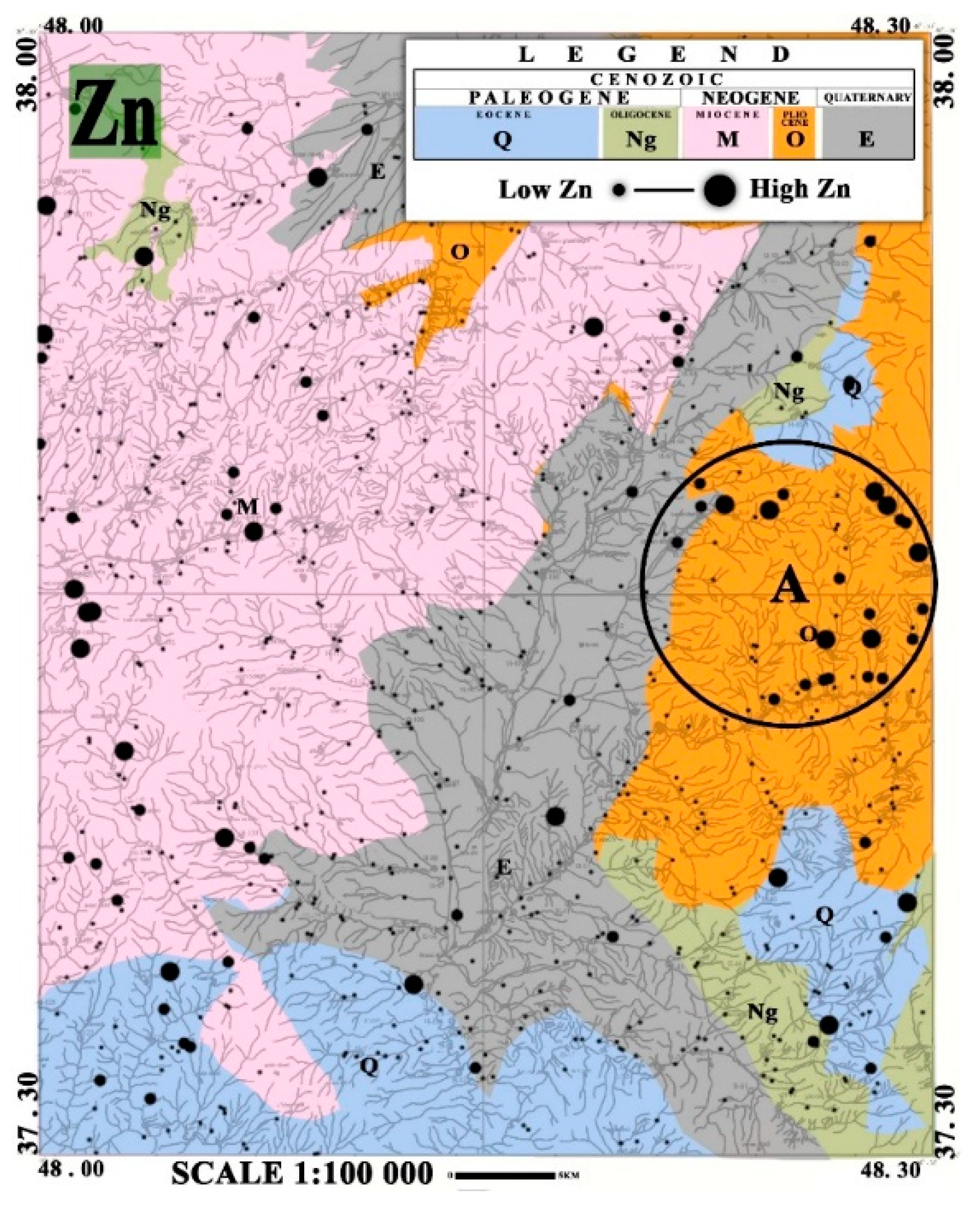
Article

Geostatistical and Remote Sensing Studies to Identify High Metallogenic Potential Regions in the Kivi Area of Iran

1
Faculty of Mining, Petroleum & Geophysics Engineering, Shahrood University of Technology, Shahrood 3619995161, Iran
2
Mining Engineering Department, Amirkabir University of Technology (Tehran Polytechnic), Tehran 1591634311, Iran
3
School of Earth Sciences & Engineering, Tomsk Polytechnic University, 634050 Tomsk, Russia
*
Author to whom correspondence should be addressed.
Minerals 2020, 10(10), 869; https://doi.org/10.3390/min10100869
Submission received: 20 August 2020 / Revised: 23 September 2020 / Accepted: 29 September 2020 / Published: 30 September 2020
(This article belongs to the Section Mineral Deposits)

Abstract

:
The Kivi area in the East Azerbaijan Province of Iran is one of the country’s highest-potential regions for metal element exploration. The primary goal herein was to process the data obtained from geochemical, geostatistical, and remote sensing tools (in the form of stream sediment samples and satellite images) to identify metallic mineralization anomalies in the region. After correcting the raw stream sediment geochemical data, single-variable statistical processing was performed, and Ti and Zn were identified as the elements with the highest degree of contrast. The relationship among these elements was further investigated using correlation and hierarchical clustering analyses. Principal component analysis was then applied to determine the principal components related to these elements, which were subsequently plotted on a regional geological map. Elements related to Ti and Zn were identified using threshold limits of anomalous samples determined via linear discriminant analysis. Lithological units and alteration patterns were detected through remote sensing investigations on Landsat-8 images. Stream sediment geochemical and remote sensing survey results identified anomalous areas of Ti and Zn in the eastern part of the study region. Our results indicate that Ti and Zn are good pathfinder elements for further exploratory investigation in this area.

Graphical Abstract

1. Introduction

Currently, geochemical exploration is deemed a critical means of generating a data layer in the mineral exploration process [1,2,3,4,5,6,7,8]. Many parameters are used in exploratory data analysis—including the full range of geochemical analysis products, the detection limits, sensitivity and accuracy of analyzers, the possibility of analyzing various geochemical variables and various data processing methods—with the goal of obtaining optimal results. Other tools relied upon by modern geochemists include software applications suitable for achieving exploration goals [9]. Once the enormous amount of information that has been entered into the exploration of geochemical data processing cycles has been digitized, experts can obtain solutions for determining high-potential and promising exploration regions [10].
The efficiency of the classic exploratory system and the current reliance on objective findings in the desert are not well-suited to exploration. Mineral exploration studies can make it easier to achieve exploration goals through a sequential process of applying statistical rules and geostatistical methods for determining the probability of mineral concentrations [11]. The Kivi area, located in the East Azerbaijan Province of Iran, has a high mineral potential of metal elements that can be better defined through geochemical investigation. Herein, the presence of the elements Ti, Zn, Mn, Cr, Sr, Mo, Cu, Ag, and As in the region was assessed using single-variable analysis and comparison with the concentration limits in stream sediments. By investigating the behavior of these elements in terms of their direct and relative relationships, several were identified as present in sufficient concentrations for potential exploitation. The principal components analysis (PCA) statistical method [12] was used to identify the lithology of the region and the mineralization marker as the primary and secondary components, respectively. To obtain more accurate results, a tree diagram of the hierarchical clustering of the elements was drawn using methods such as the squared Euclidean distance [13,14], reducing the set of elements related to mineralization in the region to Ti and Zn. The statistical communities of these two elements were then separated based on a probability diagram, and the geochemical limits of each community were determined and analysed via linear discriminant analysis (LDA) [15,16]. Finally, satellite image processing methods were used to identify the alteration and lithological units [17] in the Kivi area and the results were compared with those of other statistical studies.

2. Geological Setting of the Kivi Area

Figure 1 shows a geological map of Kivi (scale 1:100,000), including the Ardabil Province in the vicinity of the cities of Ardabil, Khalkhal and Mianeh. The study area is located in the northwestern portion of the 1:250,000 geological map of Anzali port and has the geographical coordinates 48°00′ to 48°30′ E longitude and 37°30′ to 38°00′ N latitude.
The mountain ranges in this region trend mostly north–south and have a very harsh morphology, which is clearly visible in some areas, particularly in the drainages. The region includes Eocene and young volcanic rocks in the northwest, and along the Ardabil–Kivi road there are outcrops of Neogene loose marl sediments, flat ground, and hill-like marshes. In general, there are two main mountain ranges in this area: in the eastern part of the region, the highest elevation exceeds 2600 m, and in the western part, the highest elevation is approximately 2500 m.
The Kivi area comprises three sedimentary, igneous and metamorphic units. The oldest existing sedimentary unit comprises pre-Cretaceous rocks, whereas the youngest comprises Quaternary sediments. The geological characteristics of the rock units are as follows.

2.1. Pre-Cretaceous Rocks

These are found in the western part of Haji Yousef Village along the Sangabad Road, with outcrops of metamorphic rocks including sericite schist and andalusite micaschiste.

2.2. Upper Cretaceous

Cretaceous limestone outcrops are found only in the southeastern part of the study area and are more spread out towards the east. This unit is a massive-to-thick layered silica limestone, interlayered with lime, calcareous and pyrite shales. It is grey in colour.

2.3. Eocene

The Eocene deposit in the region is a sedimentary and igneous unit that covers majority of the area and includes conglomerate, green tuffs, tuffaceous sandstone, lithic tuff, sand and tuff limestone, andesitic lava, andesitic basalt, and basalt and rhyolitic and rhyodacitic yellowish tuffs.

2.4. Oligocene

Following the vast Eocene volcanic activity with a probable gap, Oligocene rhyolite, and an andesitic eruption “related to pyrenean orogeny” activities, were continued with marl and sandstone sedimentation.

2.5. Miocene

The Miocene unit includes lahar with trachytic and dacitic fragments, perlite, dacitic, and trachytic lava with crystal tuff and vitric tuff and ignimbrite in the west of the Kivi region. In addition, there are dacite–trachyte with cherty bands, pumice tuff, lithic tuff, and white rhyodacitic volcanic ash in the northwest. Altered purple trachyandesite and andesitic vitric tuff with perthitic texture are located in the southwestern part of the region.

2.6. Quaternary

The youngest volcanic rocks in the study area are black basalts with vesicular texture that horizontally cover all older stones. Travertine outcrops with white, lemon, and red coloring occur in the mid-east of the region. This unit comprises stream sediments such as rubble and sand. The igneous rocks include dacitic, middle, and basic combinations. There are Gabbro outcrops in the eastern and northern parts of the study area. All intrusive masses cut Eocene volcanic rocks, possibly as a result of a Pyrenean (Eocene–Oligocene) orogenous phase.

3. Methodology and Materials

3.1. Exploration Geochemistry

A stream sediment sampling method in which 714 samples of stream sediments were collected from the Kivi area and analysed for the presence of 63 elements using the inductively coupled plasma-mass-spectrometry (ICP-MS) method (Table 1) was applied. Figure 2 shows the locations from which the samples were collected.

3.1.1. Raw Data Preparation Methods

Before using raw data, censored and outlier data must be identified and replaced. Such data cause problems in the application of statistical methods, which require a complete set of non-censored data. In some cases, such as the separation of anomalies from the background and relative measurement, the presence of censored data produces inappropriate evaluation results. If the censored data are identified and replaced, the amount of background and the intensity of anomalies can be calculated with high accuracy [18].
Outlier data have the same effect as censored data in terms of generating errors from geochemical data. Outlier data, which are data points that significantly deviate from other observed data [19,20], typically have two sources: sampling error and errors in laboratory measurement and analysis [21]. Outlier data can cause serious problems in statistical investigation and the future decisions based on its results [22].
Several methods can be used to detect and replace censored and outlier data. Herein, a simple method was used to replace censored data in which values below the analyzer detection limit were replaced by 3/4 of the recorded values. However, this method has a fundamental problem in that it is not affected by the statistical parameters of the data community and is merely a function of the sensitivity of the measurement method [18,23].
The Doerffel method was used to identify and replace outlier data [22]. Doerffel developed a graph for determining the threshold of outlier data values at two levels of accuracy: 5% and 1% (see Figure 4) [24,25].
To perform the Doerffel test, the averages ( x ¯ ) and standard deviations of the data points were calculated regardless of the maximum data value. The largest data value (xA) was considered to be outside of the range if the following equation was satisfied:
x A x ¯ + s . g ,
where “g” is the threshold limit for outlier values, which can be calculated using the graph shown in Figure 3.

3.1.2. Correlation Investigations of Raw Data

By applying correlation analysis to the raw data, the relationship between each set of two elements could be calculated. Using these results, the relationship between the mineralization and mobility of different elements can be identified [25]. Correlation analysis is useful in predicting the behaviour of elements in a region [26], and a behavioral analysis of different elements can be used to determine the relationship between mineralization and geochemical halos [27,28].

3.1.3. Hierarchical Clustering Analysis Method (HCA)

The hierarchical clustering analysis (HCA) method was used to divide elements into clusters within which related elements could be grouped. HCA can be applied using two different clustering strategies—the agglomerative and divisive methods—which are shown in Figure 4 [29].

3.1.4. Principal Components Analysis (PCA)

The principal components method (PCA) method is used to reduce the size of a dataset. By applying this method, the overall set of data can be replaced by data that are most highly correlated with each other [30,31]. The PCA method is based on the calculation of eigenvalues and eigenvectors to reduce the dimensionality of the dataset [32]. The new data generated by PCA will therefore be independent of each other [18]. To obtain the eigenvalues and eigenvectors, the bands correlation matrix must be calculated first [33].

3.1.5. Linear Discriminant Analysis (LDA)

LDA is a community separation technique [34] based on the number of categories that include interdependent variables [35]. Figure 5 presents the steps of LDA [36,37].
Figure 6 shows the application of linear classification boundaries when a dataset including two variable groups is modeled using LDA [28].

3.2. Exploratory Remote Sensing

Herein, remote sensing was performed using the Landsat 8 satellite data for the Kivi region. Methods used for remote sensing on raw corrected satellite data include band combinations and multiplications, band ratios and developed selective PCA (DSPCA), which is applied to the shortwave infrared (SWIR) and near infrared (NIR) spectral bands of Landsat-8 [38,39].
Lithological units can be separated and high-potential mineral areas can be identified using advanced remote sensing (RS) methods in the SWIR and NIR spectral bands of the satellite [40,41,42,43]. The accuracy of the images used in this study ranged between 15 and 100 m [44].

Remote Sensing Data

A cloud-free remotely sensed dataset from the Landsat-8 sensor (October 2017) covering the Kivi area was obtained through the United States Geological Survey and its metadata were used to transform recorded digital number values to radiance values [45]. The internal average relative reflectance (IARR) [46] was used as an atmospheric correction technique; to normalize images to a scene average for obtaining reflectance from the radiance data: the IARR calibration was applied [47] and the images were then resized to the research area.

4. Results and Discussion

4.1. Exploratory Geochemistry

4.1.1. Censored and Outlier Data

Given the large quantity of censored data in some of the elements, censored elements were, to the greatest extent possible, replaced with values obtained using the Doerffel method, whereas elements with very high values were removed. Table 2 lists the remaining elements following the initial refinement.

4.1.2. Single-Variable Initial Analysis

After analyzing the data in single-variable form, as listed in Table 3, the most important elements for the study were selected according to a histogram and probability diagram of the overall dataset.
In cases of mineralization or contamination of samples through anthropogenic activities in the region, the mean values did not correspond to the median values, which deviated to the left or right of the mean. In this condition, there was no symmetry in the histogram. In the probability diagram, the data did not lie along a straight line. Consequently, the important elements were separated from other elements owing to their high values relative to the background as well as the skewness, Kurtosis, and asymmetry of the histogram and the non-linearity of the probability graph. Based on the results listed in Table 3, which presents a statistical analysis of the elements and the anomalous limits of each element in the stream sediments, eight important elements were selected and arranged in order of priority. The elements suspected of being anomalous to the area are also listed in the Table 3. Ti and Zn were identified as the most important elements in the region based on the statistical parameters and anomalous limits of the stream sediments. Probability charts and non-logarithmic histograms of Ti and Zn are plotted in Figure 7 and Figure 8, respectively.

4.1.3. Correlation Coefficients and Hierarchical Clustering

A lack of dependence between variables is the main criterion in single-variable and related statistical studies. However, in practice, such independence is not found in nature because various factors, such as genetics, effectively dominate the relationship and dependence between variables. Thus, the value of dependence between elements can be numerically expressed in terms of the correlation or geochemical correlation coefficient. To determine the relationship between the elements in the stream sediment samples, a correlation coefficient matrix between the elements was developed (Table 4).
Based on the determined correlations, clustering was performed using the squared Euclidean distance after normalizing the data to values between zero and one, as shown in Figure 9, in which the hierarchical diagram clearly groups Ti and Zn into one cluster.

4.1.4. Principal Components Analysis (PCA)

As can be observed in Figure 10, six components were found to be appropriate. The values in red indicate the most important elements in each component. The first component describes the region’s lithology whereas the second describes the mineralization (Table 5).

4.1.5. Separating Communities on the Probability Chart

The Ti and Zn communities were separated using a probability diagram to determine the boundaries of the geochemical threshold. The breakpoints of the probability chart, which represent changes in trend, were considered community boundaries [26]. Probability charts of Ti and Zn are shown in Figure 11 and Figure 12, respectively, and anomalous values for the two elements are listed in Table 6.

4.1.6. Linear Discriminant Analysis (LDA)

The LDA method was applied to separate the domains of Ti and Zn using the community separation results.

Community Separation Based on Ti Element Classifications

Three communities were separated for the Ti element (Figure 13); the communities and their element names are shown in Figure 14. The validity of this separation is provided in Table 7.

Community Separation Based on Zn Element Classification

Three communities were separated for the Zn element (Figure 15); Figure 16 shows them with their element names in Figure 16. The validity of this separation is provided in Table 8.
The results listed in Table 8 indicate that the separation was performed with a high degree of accuracy. For example, 91.5% of samples are in the first group while only 8.5% are in the second group; the third group contains no data. This categorization can be considered for its general accuracy with respect to the high accuracy obtained in groups 1 and 2 and can be used for clustering.

4.1.7. Anomaly Maps

Anomalous samples obtained from the results were placed on the regional topographic map (Figure 17, Figure 18 and Figure 19).
The results of statistical and geostatistical investigations were then used to identify the main anomalies for the Ti and Zn elements (Figure 20 and Figure 21, respectively), and the identified Ti and Zn anomalies were plotted on the regional lithology map (Figure 22 and Figure 23, respectively).

4.2. Exploratory Remote Sensing

4.2.1. Band Math and Band Ratios

Operational land imager (OLI) data were used to identify hydrothermal alterations in the region. To map the lithology, band ratios of 6/7, 6/4, and 4/2 were assigned to the red, green, and blue (RGB) colors, respectively, as false color composite (FCC) ratios (Figure 24).
The results for RGB values of 7, 5, and 3 are presented in Figure 24. In addition to the geological map of Kivi in Figure 25, in which the dark violet colors represent basalt, andesite, and thick bedded volcanic conglomerate rock units, this image robustly separates the major lithological units within the region.

4.2.2. Principal Components Analysis (PCA)

Figure 26 shows the first three general principal components (PCs) in RGB false colour format. The image contains nearly all spectral information gathered in nine OLI bands, and the accumulation of spectral information helps to represent the discriminated rock unites in different colors.
DSPCA was used to map aluminum (AL)-hydroxy (OH)-bearing altered rocks. For this purpose, bands 2, 5, 6, and 7 were selected; the statistical results are listed in Table 9.
Considering the PC loadings for seventh (+0.68) and sixth bands (−0.66), OH-bearing altered minerals were provided in PC 4 to enhance the altered zones (Table 9). Figure 27 shows the altered areas from PC 4 mapped in red.

5. Conclusions

Based on the results of this study on geostatistical data and remote sensing, we present the following conclusions.
  • Clearly, the Kivi region is a high-potential area for metallogenic exploration.
  • Ti and Zn were identified as anomalous elements based on single-variable studies and comparison with the background threshold limits of stream sediment. According to the geological information, there are other metal elements in the region, including Cu in basalt; however, their presence in the stream sediment samples did not reach the anomalous threshold limit.
  • An investigation of the relationship between the two identified elements using hierarchical and correlation analyses revealed a strong positive correlation between the two elements. The hierarchical clustering also confirmed that the Ti and Zn elements are the primary anomalous elements in the region.
  • Different communities of Ti and Zn elements were separated using a probability diagram and the results were subjected to LDA analysis to obtain separate groupings between Ti and Zn and their associated elements. The results were estimated through cross-validation with more than 90% validity.
  • PCA results indicated that the first and second components represent the lithology and mineralization of the region, respectively.
  • Based on geological mapping and RS investigation, the trend of identified anomalies was found to follow volcanic and plutonic calc–alkaline rocks belonging to the Eocene epoch, including basalt, andesite, and thick bedded volcanic conglomerate rock units in addition to the alluvial deposits resulting from their erosion and weathering over time.
  • Minerals of economic interest containing Ti metal include ilmenite and rutile. Given the presence of these minerals in the area, there is a possibility of ore deposits. Other Ti anomalies with no economic value can be derived from pyroxenes and biotite. In the future, heavy mineral studies should be conducted in regions identified as anomalies to identify the types of minerals containing Ti.

Author Contributions

A.S. conceived and designed the study and wrote the initial draft of the manuscript. A.S. and M.Z. collected the samples and conducted sample preparation for analytical work. A.S., M.Z., and A.H. analyzed the data, and conducted processing graphic and analytical work. T.T. revised and corrected the final version. All authors have read and agreed to the published version of the manuscript.

Funding

This research received no external funding.

Acknowledgments

Laboratory investigations were carried out at Tomsk Polytechnic University within the framework of a Competitiveness Enhancement Program Grant. We thank the editor and three anonymous reviewers for their constructive criticisms and revisions, which led to improvement of the manuscript.

Conflicts of Interest

The authors declare no conflict of interest.

References

  1. Zhang, B.; Wang, X.; Ye, R.; Zhou, J.; Liu, H.; Liu, N.; Han, Z.; Lin, X.; Wang, Z. Geochemical exploration for concealed deposits at the periphery of the Zijinshan copper–gold mine, southeastern China. J. Geochem. Explor. 2015, 157, 184–193. [Google Scholar] [CrossRef]
  2. Gandhi, S.M.; Sarkar, B.C.; Gandhi, S.M.; Sarkar, B.C. Geochemical exploration. In Essentials of Mineral Exploration and Evaluation; Elsevier: Amsterdam, The Netherlands, 2016; pp. 125–158. [Google Scholar]
  3. Zuo, R.; Carranza, E.J.M.; Wang, J. Spatial analysis and visualization of exploration geochemical data. Earth Sci. Rev. 2016, 158, 9–18. [Google Scholar] [CrossRef]
  4. Cherkasova, T.; Chernishov, A.; Goltsova, Y.; Timkin, T.; Abramova, R. Petrogenetic characteristics of mafic-ultramafic massifs in Nizhne-Derbinsk complex (East Sayan Mountains). IOP Conf. Ser. Earth Environ. Sci. 2015, 27, 012002. [Google Scholar] [CrossRef]
  5. Yousefi, M. Recognition of an enhanced multi-element geochemical signature of porphyry copper deposits for vectoring into mineralized zones and delimiting exploration targets in Jiroft area, SE Iran. Ore Geol. Rev. 2017, 83, 200–214. [Google Scholar] [CrossRef]
  6. Ziaii, M.; Safari, S.; Timkin, T.V.; Voroshilov, V.; Yakich, T. Identification of geochemical anomalies of the porphyry–Cu deposits using concentration gradient modelling: A case study, Jebal-Barez area, Iran. J. Geochem. Explor. 2019, 199, 16–30. [Google Scholar] [CrossRef]
  7. Saadati, H.; Afzal, P.; Torshizian, H.; Solgi, A. Geochemical exploration for lithium in NE Iran using the geochemical mapping prospectivity index, staged factor analysis, and a fractal model. Geochem. Explor. Environ. Anal. 2020. [Google Scholar] [CrossRef]
  8. Timkin, T.V.; Voroshilov, V.; Askanakova, O.; Cherkasova, T.; Chernyshov, A.; Korotchenko, T. Estimating gold-ore mineralization potential within Topolninsk ore field (Gorny Altai). IOP Conf. Series: Earth Environ. Sci. 2015, 27, 12010. [Google Scholar] [CrossRef]
  9. Shirazy, A.; Shirazi, A.; Ferdossi, M.H.; Ziaii, M.; Adel, S.; Aref, S.; Mohammad, H.F.; Mansour, Z. Geochemical and geostatistical studies for estimating gold grade in tarq prospect area by k-means clustering method. Open J. Geol. 2019, 9, 306–326. [Google Scholar] [CrossRef] [Green Version]
  10. Shirazi, A.; Shirazy, A.; Saki, S.; Hezarkhani, A. Introducing a software for innovative neuro-fuzzy clustering method named NFCMR. Glob. J. Comput. Sci. Theory Res. 2018, 8, 62–69. [Google Scholar] [CrossRef]
  11. Khakmardan, S.; Shirazi, A.; Shirazy, A.; Hosseingholi, H. Copper oxide ore leaching ability and cementation behavior, mesgaran deposit in Iran. Open J. Geol. 2018, 8, 841–858. [Google Scholar] [CrossRef] [Green Version]
  12. Cheng, Q.; Bonham-Carter, G.; Wang, W.; Zhang, S.; Li, W.; Qinglin, X. A spatially weighted principal component analysis for multi-element geochemical data for mapping locations of felsic intrusions in the Gejiu mineral district of Yunnan, China. Comput. Geosci. 2011, 37, 662–669. [Google Scholar] [CrossRef]
  13. Templ, M.; Filzmoser, P.; Reimann, C. Cluster analysis applied to regional geochemical data: Problems and possibilities. Appl. Geochem. 2008, 23, 2198–2213. [Google Scholar] [CrossRef]
  14. Liu, Y.; Zhou, K.; Carranza, E.J.M. Compositional balance analysis for geochemical pattern recognition and anomaly mapping in the western Junggar region, China. Geochem. Explor. Environ. Anal. 2018, 18, 263–276. [Google Scholar] [CrossRef]
  15. Roshani, P.; Mokhtari, A.R.; Tabatabaei, S.H. Objective based geochemical anomaly detection—Application of discriminant function analysis in anomaly delineation in the Kuh Panj porphyry Cu mineralization (Iran). J. Geochem. Explor. 2013, 130, 65–73. [Google Scholar] [CrossRef]
  16. Grunsky, E.C.; de Caritat, P. State-of-the-art analysis of geochemical data for mineral exploration. Geochem. Explor. Environ. Anal. 2020, 20, 217–232. [Google Scholar] [CrossRef]
  17. Ni, P.; Li, S.-N.; Bao, T.; Zheng, W.-Y.; Wang, G.-G.; Xiang, H.-L.; Chi, Z.; Pan, J.-Y.; Huang, B.; Ding, J.-Y.; et al. Mapping of fluid, alteration and soil geochemical anomaly as a guide to regional mineral exploration for the Dehua gold orefield of Fujian Province, SE China. Geochem. Explor. Environ. Anal. 2018, 19, 74–90. [Google Scholar] [CrossRef]
  18. Hassanipak, A.A.; Sharafeddin, M. Exploration Data Analysis; Tehran University Press: Tehran, Iran, 2005; Volume 1. (In Persian) [Google Scholar]
  19. Grubbs, F.E. Procedures for detecting outlying observations in samples. Technometrics 1969, 11, 1–21. [Google Scholar] [CrossRef]
  20. Madala, G.S. Introduction to Econometrics, 2nd ed.; Maxmillan Publishing Company: New York, NY, USA, 1992. [Google Scholar]
  21. Kalisch, M.; Michalak, M.; Sikora, M.; Wróbel, Ł.; Przystalka, P. Influence of outliers introduction on predictive models quality. In Proceedings of the 12th International Conference, BDAS 2016, Ustroń, Poland, 31 May–3 June 2016; Volume 613, pp. 79–93. [Google Scholar]
  22. Shirazi, A.; Shirazy, A.; Saki, S.; Hezarkhani, A. Geostatistics studies and geochemical modeling based on core data, sheytoor iron deposit, Iran. J. Geol. Resour. Eng. 2018, 6, 124–133. [Google Scholar] [CrossRef]
  23. Hassani Pak, A. Geostatistics; University of Tehran: Tehran, Iran, 1998. (In Persian) [Google Scholar]
  24. Yousefi, M. General and Detailed Exploration of Iron Ore Anomalies of Iran’s Central Plateau, 5a Anomlay (Sheytoor-Gazestan); Madankav Engineering Co.: Tehran, Iran, 2016. [Google Scholar]
  25. Chatfield, C.; Collins, A.J.; Chatfield, C. Introduction to Multivariate Analysis; Springer: New York, NY, USA, 2018. [Google Scholar] [CrossRef]
  26. Mertler, C.A.; Reinhart, R.V. Advanced and Multivariate Statistical Methods: Practical Application and Interpretation, 5th ed.; Routledge: London, UK, 2016; p. 374. [Google Scholar]
  27. Rollinson, H.R. Using Geochemical Data: Evaluation, Presentation, Interpretation; Taylor and Francis: Oxfordshire, UK, 2014. [Google Scholar]
  28. Alahgholi, S.; Shirazy, A.; Shirazi, A. Geostatistical studies and anomalous elements detection, Bardaskan area, Iran. Open J. Geol. 2018, 8, 697–710. [Google Scholar] [CrossRef] [Green Version]
  29. Rokach, L.; Maimon, O. Clustering methods. In Data Mining and Knowledge Discovery Handbook; Springer: New York, NY, USA, 2005; pp. 321–352. [Google Scholar]
  30. Manuel, R.; Brito, G.; Chichorro, M.; Rosa, C. Remote sensing for mineral exploration in central Portugal. Minerals 2017, 7, 184. [Google Scholar] [CrossRef] [Green Version]
  31. Wang, G.; Du, W.; Carranza, E.J.M. Remote sensing and GIS prospectivity mapping for magmatic-hydrothermal base- and precious-metal deposits in the Honghai district, China. J. Afr. Earth Sci. 2017, 128, 97–115. [Google Scholar] [CrossRef]
  32. Gómez-Palacios, D.; Torres, M.A.; Reinoso, E. Flood mapping through principal component analysis of multitemporal satellite imagery considering the alteration of water spectral properties due to turbidity conditions. Geomat. Nat. Hazards Risk 2016, 8, 607–623. [Google Scholar] [CrossRef]
  33. Soe, M.; Kyaw, T.A.; Takashima, I. Application of Remote Sensing Techniques on Iron Oxide Detection from ASTER and Landsat Images of Tanintharyi Coastal Area, Myanmar. Available online: https://citeseerx.ist.psu.edu/viewdoc/download?doi=10.1.1.598.998&rep=rep1&type=pdf (accessed on 25 August 2020).
  34. Chien, N.P.; Lautz, L.K. Discriminant analysis as a decision-making tool for geochemically fingerprinting sources of groundwater salinity. Sci. Total Environ. 2018, 618, 379–387. [Google Scholar] [CrossRef] [PubMed]
  35. Yakubu, I.; Dinye, R.; Buor, D.; Iddrisu, W.A.; Yakubu, I.; Dinye, R.; Buor, D.; Iddrisu, W.A. Discriminant analysis of demand-side roadblocks to financial inclusion in Northern Ghana. J. Math. Financ. 2017, 7, 718–733. [Google Scholar] [CrossRef] [Green Version]
  36. Friedman, J.H. Regularized discriminant analysis. J. Am. Stat. Assoc. 1989, 84, 165–175. [Google Scholar] [CrossRef]
  37. Klecka, W. Discriminant analysis. Adv. Neural Inform. Proc. Syst. 1980, 17, 1569–1576. [Google Scholar] [CrossRef]
  38. Shirazi, A.; Shirazy, A.; Karami, J. Remote sensing to identify copper alterations and promising regions, Sarbishe, South Khorasan, Iran. Int. J. Geol. Earth Sci. 2018, 4, 36–52. [Google Scholar]
  39. Adiri, Z.; Lhissou, R.; El Harti, A.; Jellouli, A.; Chakouri, M. Recent advances in the use of public domain satellite imagery for mineral exploration: A review of Landsat-8 and Sentinel-2 applications. Ore Geol. Rev. 2020, 117, 103332. [Google Scholar] [CrossRef]
  40. Abrams, M. The advanced spaceborne thermal emission and reflection radiometer (ASTER): Data products for the high spatial resolution imager on NASA’s Terra platform. Int. J. Remote. Sens. 2000, 21, 847–859. [Google Scholar] [CrossRef]
  41. Irons, J.R.; Dwyer, J.; Barsi, J.A. The next Landsat satellite: The Landsat data continuity mission. Remote. Sens. Environ. 2012, 122, 11–21. [Google Scholar] [CrossRef] [Green Version]
  42. Markham, B.; Storey, J.; Williams, D.; Irons, J. Landsat sensor performance: History and current status. IEEE Trans. Geosci. Remote. Sens. 2004, 42, 2691–2694. [Google Scholar] [CrossRef]
  43. Morfitt, R.; Barsi, J.A.; Levy, R.; Markham, B.; Micijevic, E.; Ong, L.; Scaramuzza, P.; Vanderwerff, K. Landsat-8 operational land imager (OLI) radiometric performance on-orbit. Remote Sens. 2015, 7, 2208–2237. [Google Scholar] [CrossRef] [Green Version]
  44. Pour, A.B.; Hashim, M. Hydrothermal alteration mapping from Landsat-8 data, Sar Cheshmeh copper mining district, south-eastern Islamic Republic of Iran. J. Taibah Univ. Sci. 2015, 9, 155–166. [Google Scholar] [CrossRef]
  45. Safari, M.; Maghsoudi, A.; Pour, A.B. Application of Landsat-8 and ASTER satellite remote sensing data for porphyry copper exploration: A case study from Shahr-e-Babak, Kerman, south of Iran. Geocarto Int. 2017, 33, 1186–1201. [Google Scholar] [CrossRef]
  46. Aspinall, R.J.; Marcus, W.; Boardman, J.W. Considerations in collecting, processing, and analysing high spatial resolution hyperspectral data for environmental investigations. J. Geogr. Syst. 2002, 4, 15–29. [Google Scholar] [CrossRef]
  47. Shirazi, A.; Hezarkhani, A.; Shirazy, A. Remote sensing studies for mapping of iron oxide regions, South of Kerman, IRAN. Int. J. Sci. Eng. Appl. 2018, 7, 45–51. [Google Scholar] [CrossRef]
Figure 1. Simplified geological map of the Kivi area with streams. (Left: by Time, Right: by lithology).
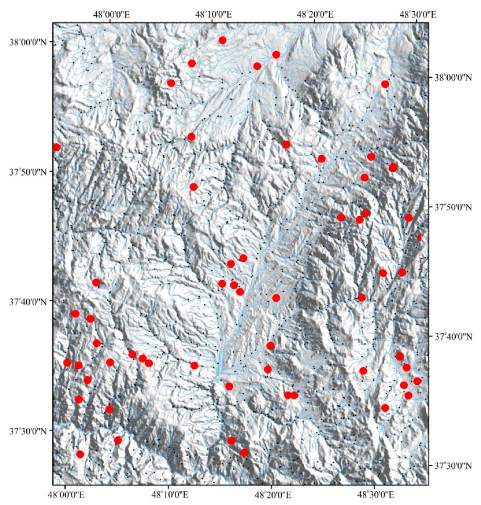
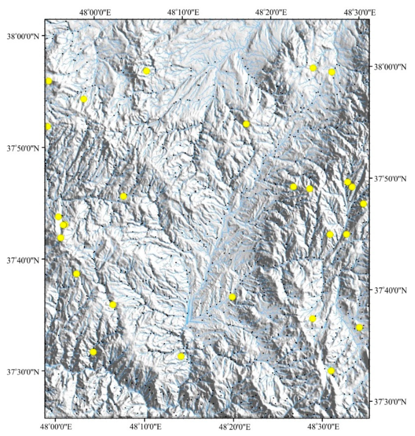
Minerals 10 00869 g001
Figure 2. Topographical map showing the location of stream sediment samples in the Kivi area.
Minerals 10 00869 g002
Figure 3. The threshold of outlier values (g) as a function of the sample number (n) and the level of accuracy.
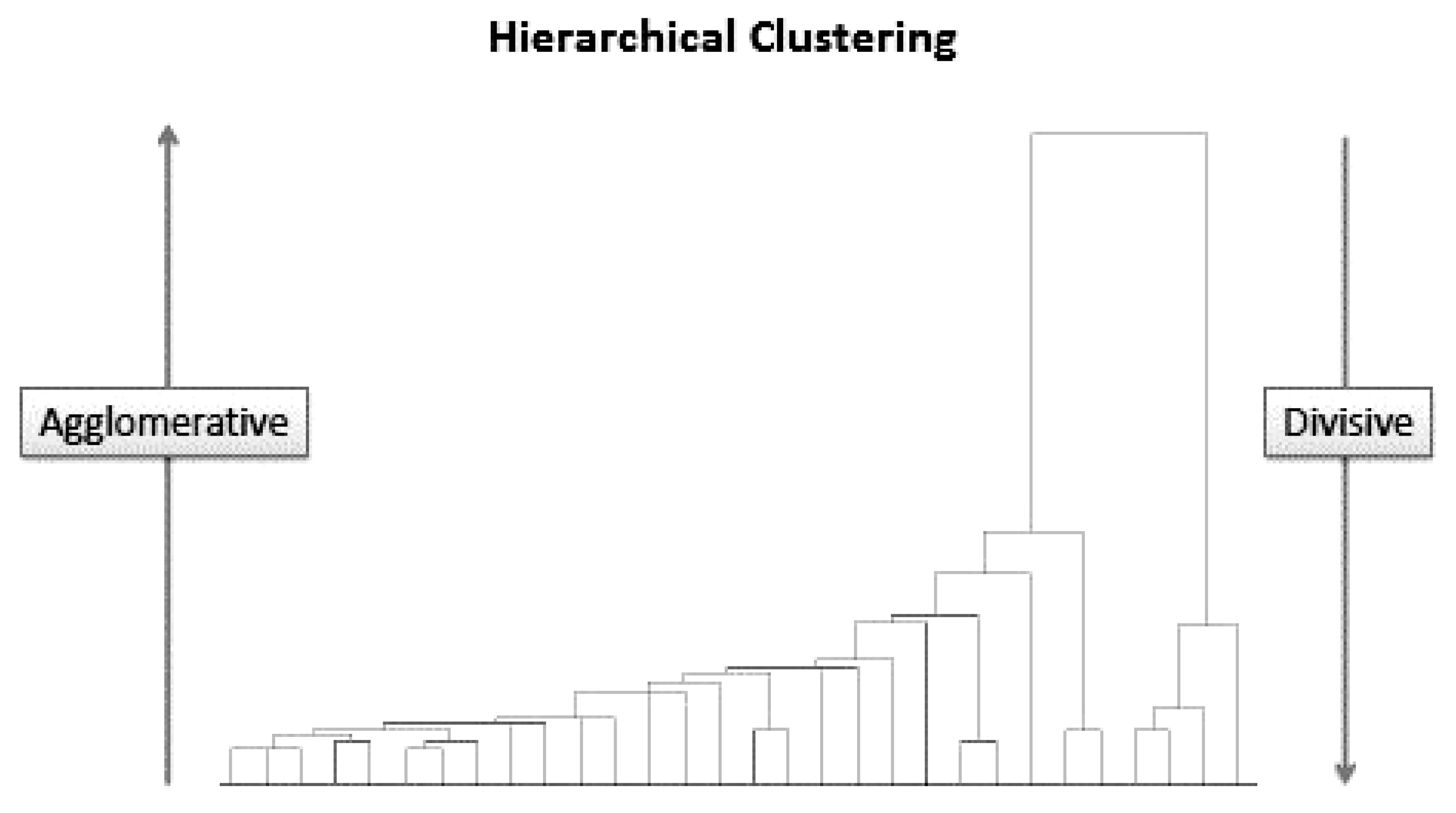
Minerals 10 00869 g003
Figure 4. Hierarchical clustering strategies.
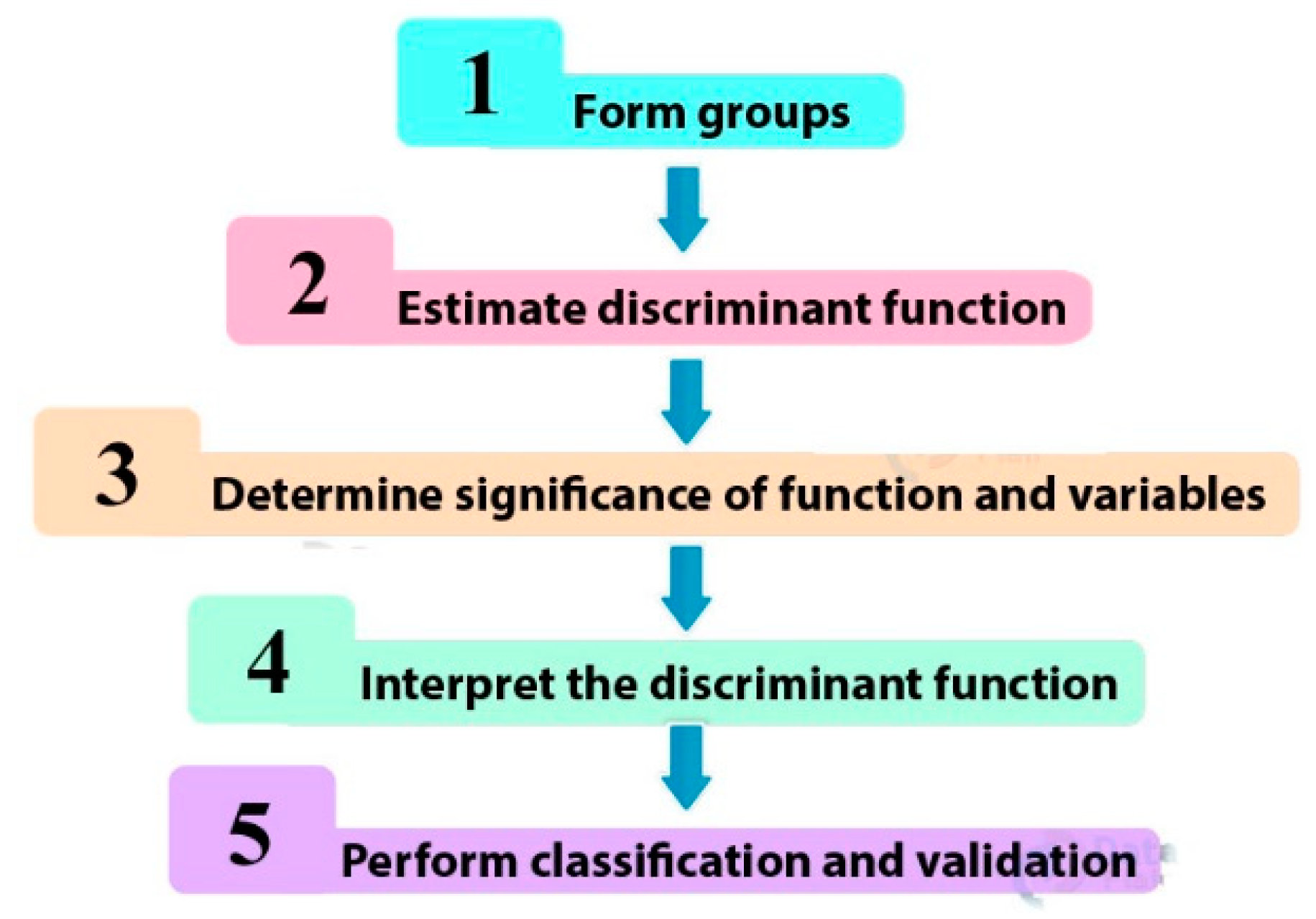
Minerals 10 00869 g004
Figure 5. Steps in discriminant analysis.
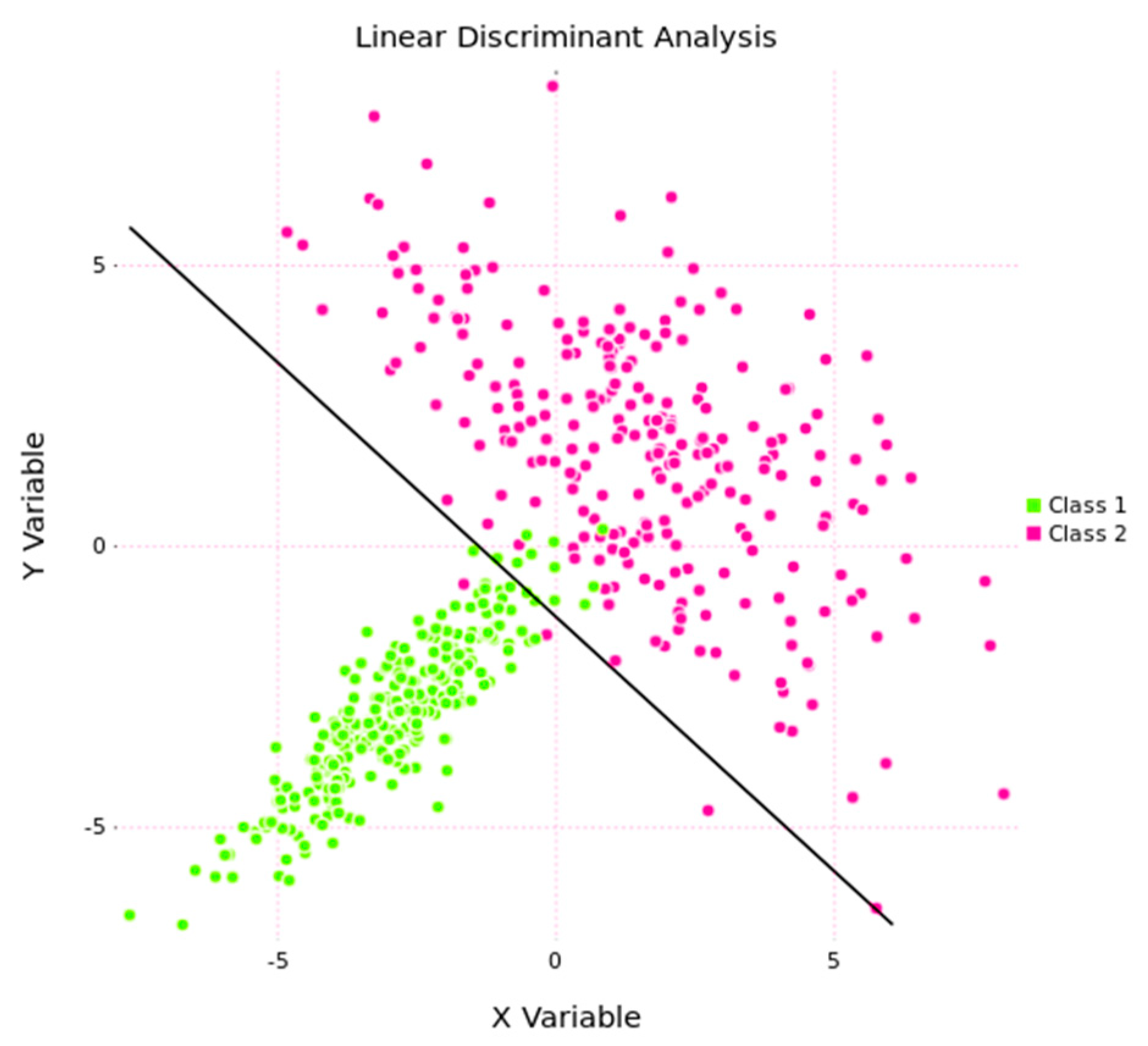
Minerals 10 00869 g005
Figure 6. Schematic image of the separation of two communities by linear discriminant analysis (LDA) method.
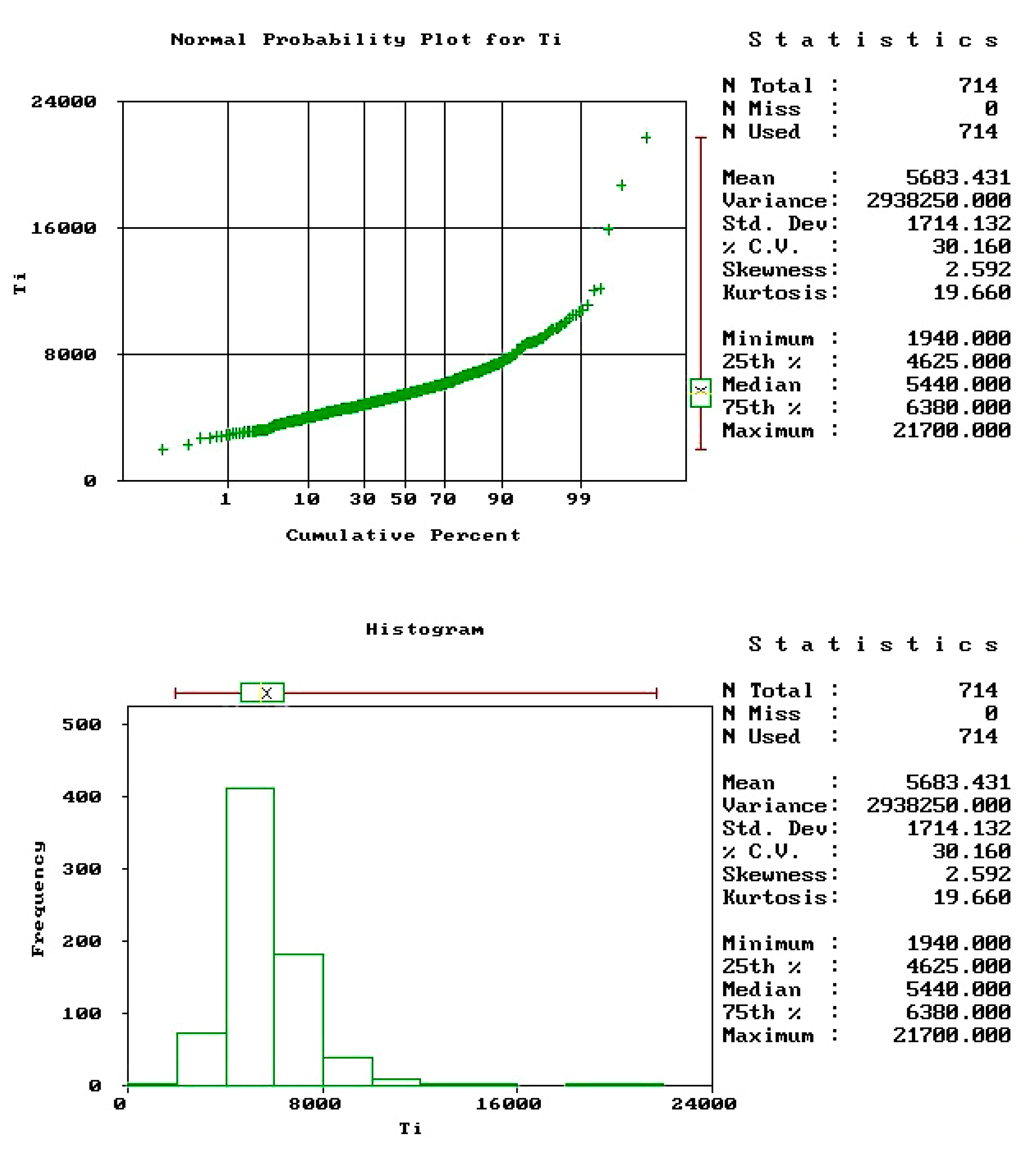
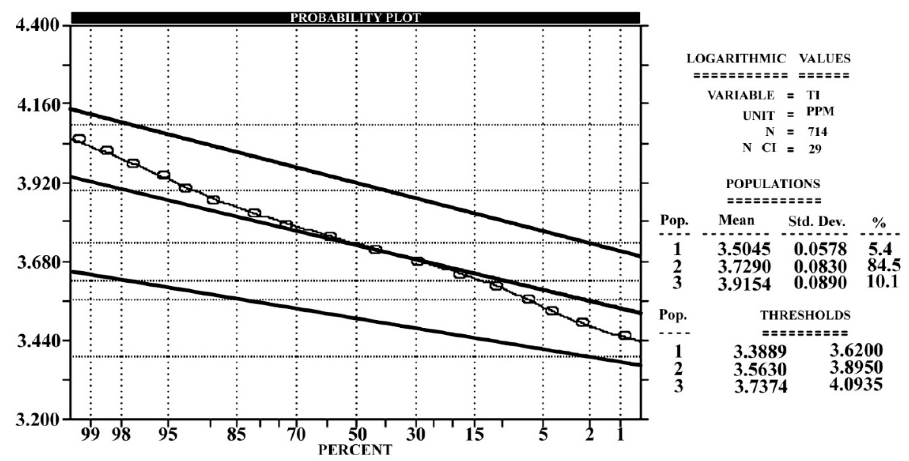
Minerals 10 00869 g006
Figure 7. Probability diagram and in non-logarithmic histogram for Ti element.
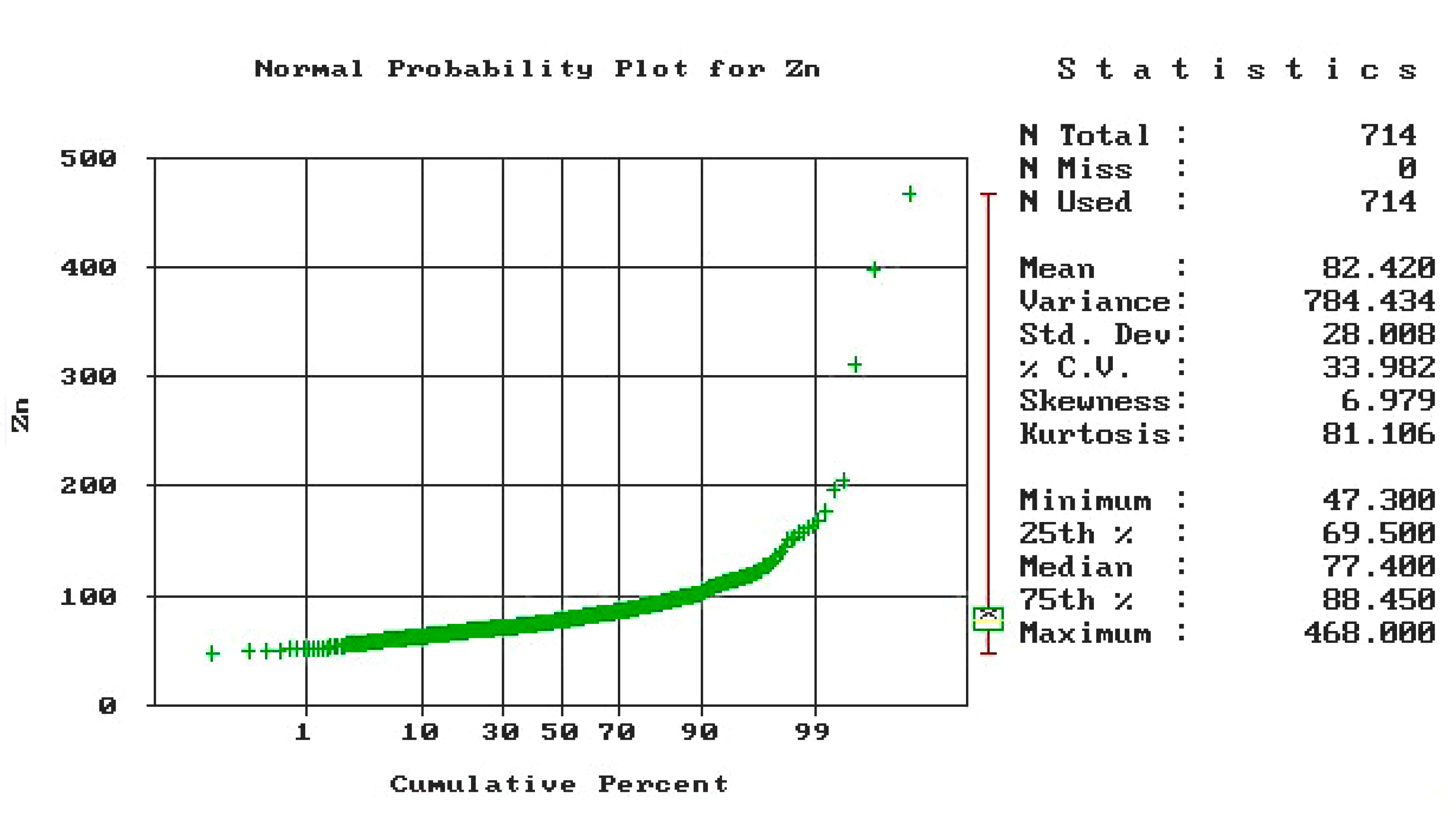
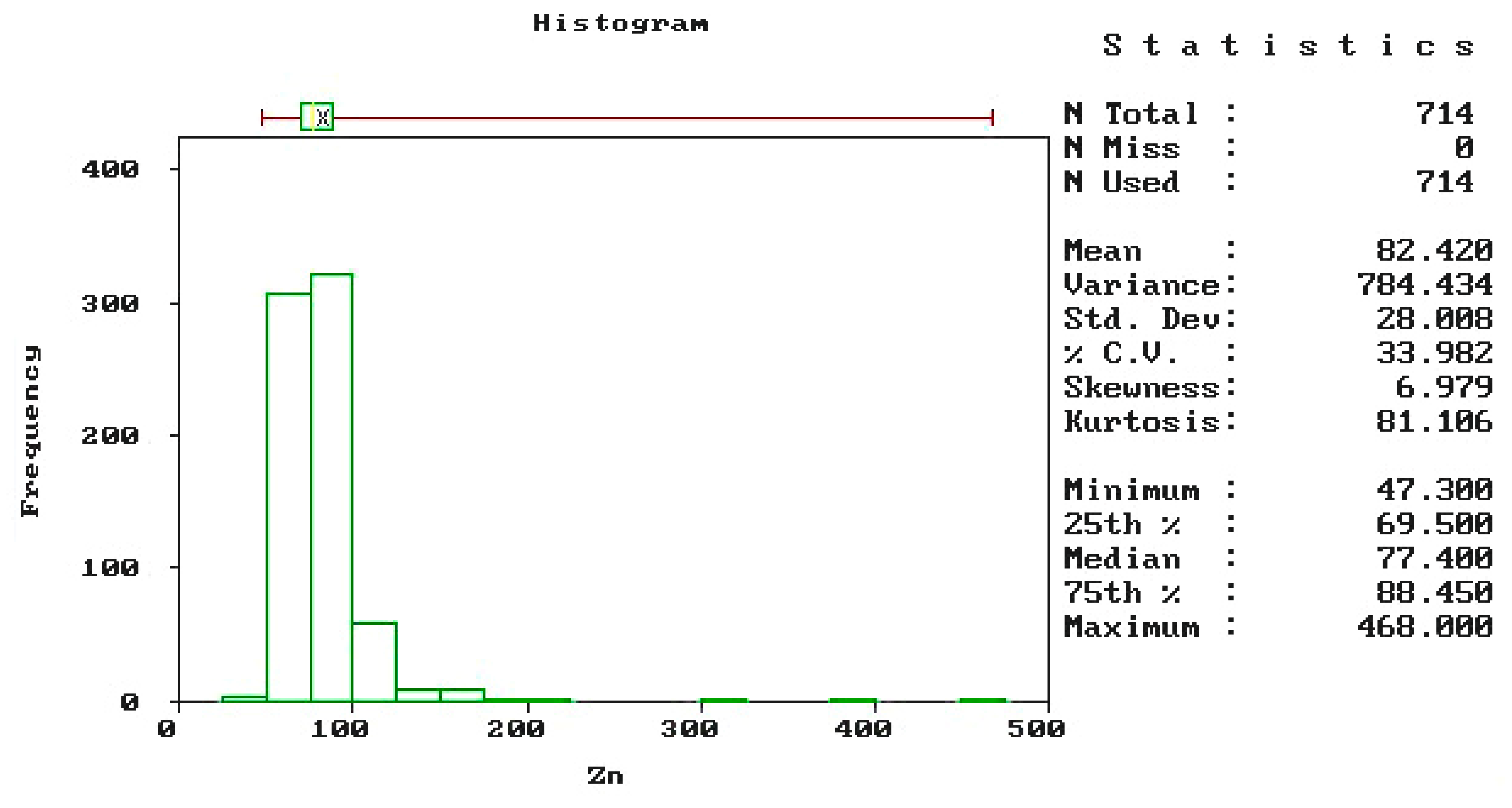
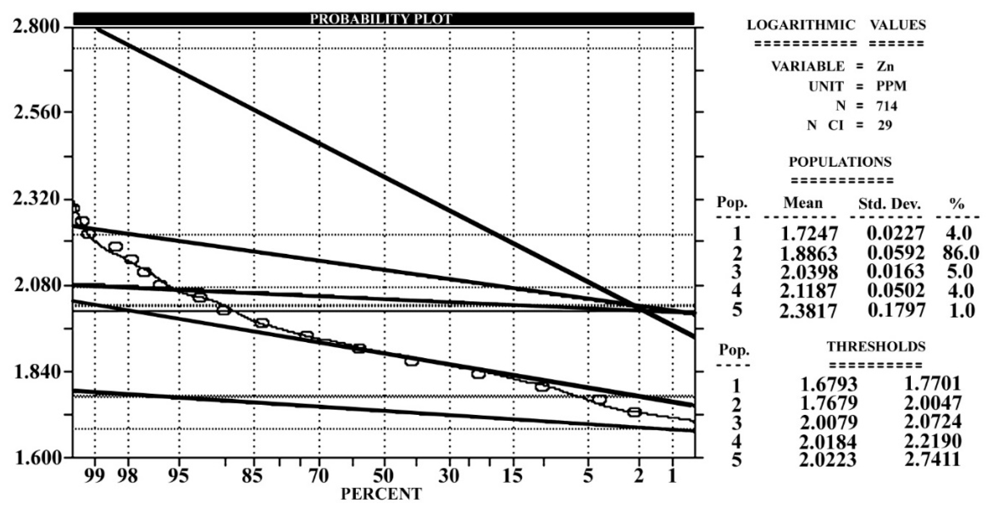
Minerals 10 00869 g007
Figure 8. Probability diagram and in non-logarithmic histogram for Zn element.
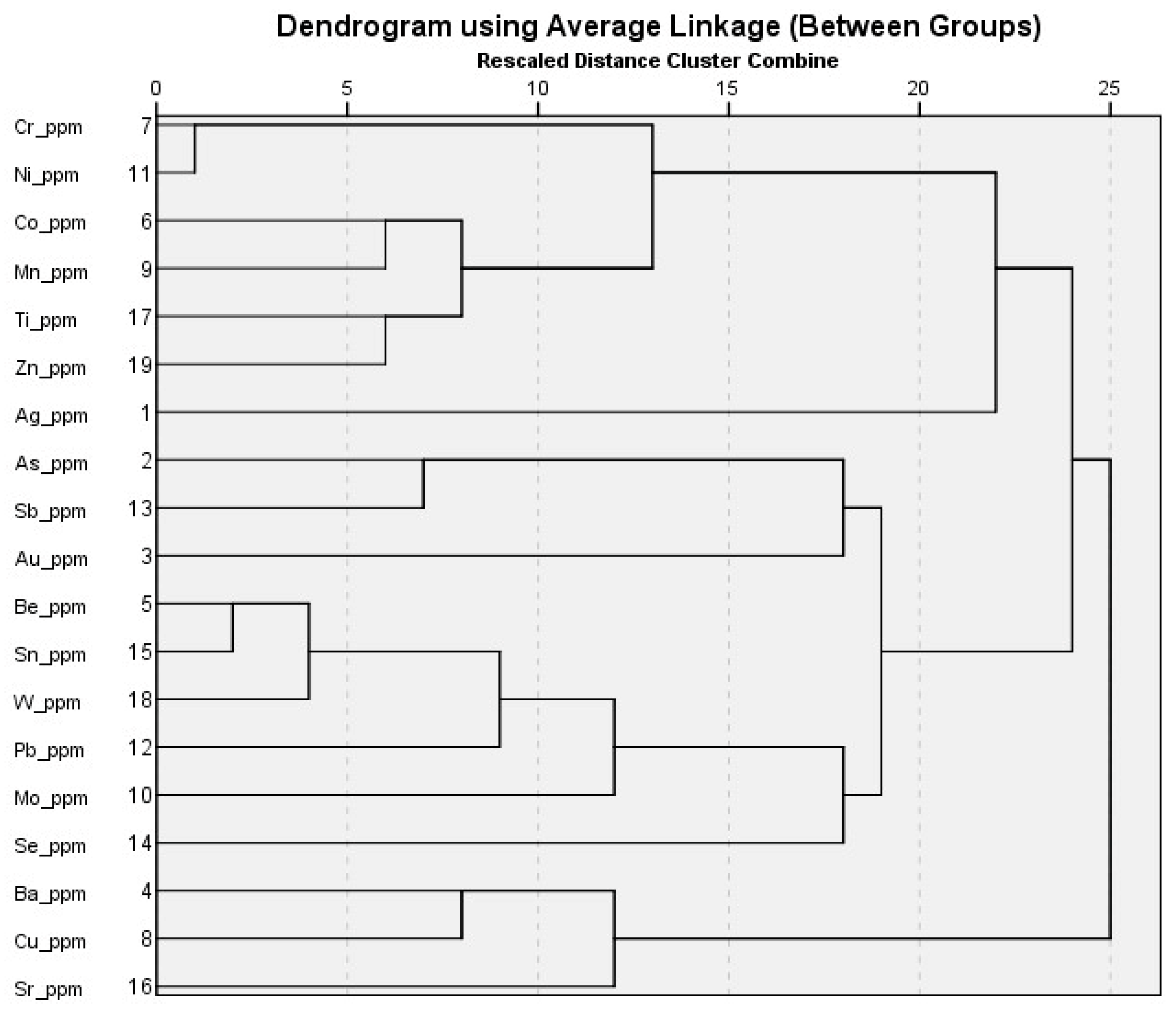
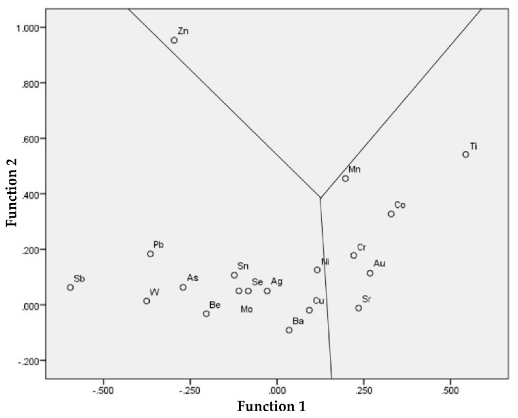
Minerals 10 00869 g008aMinerals 10 00869 g008b
Figure 9. Hierarchical diagram of the elements in the Kivi area.
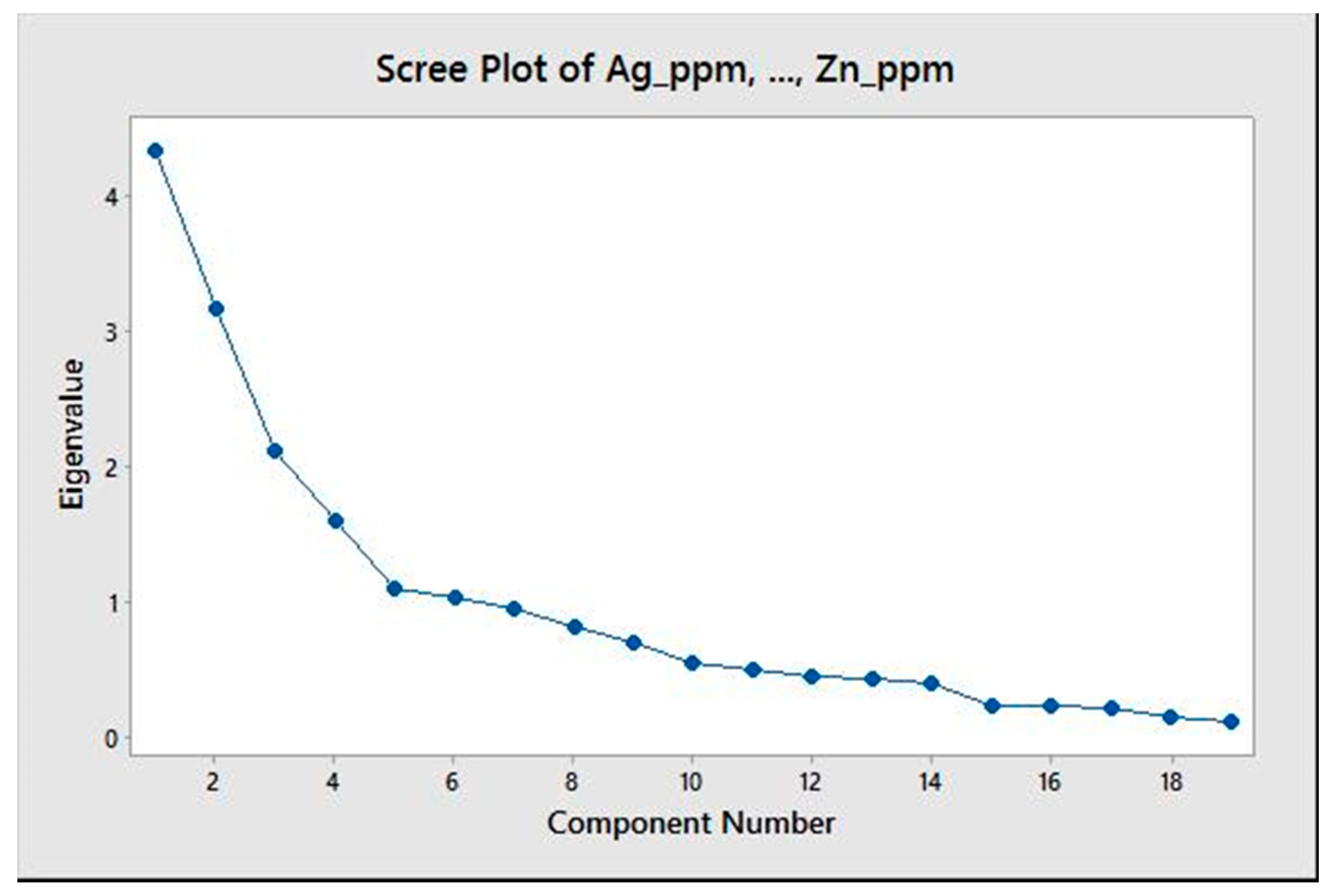
Minerals 10 00869 g009
Figure 10. The scree plot of Principal Components Analysis (PCA) on elements.
Minerals 10 00869 g010
Figure 11. Separation of titanium element communities on the probability diagram.
Minerals 10 00869 g011
Figure 12. Separation of zinc element communities on the probability diagram.
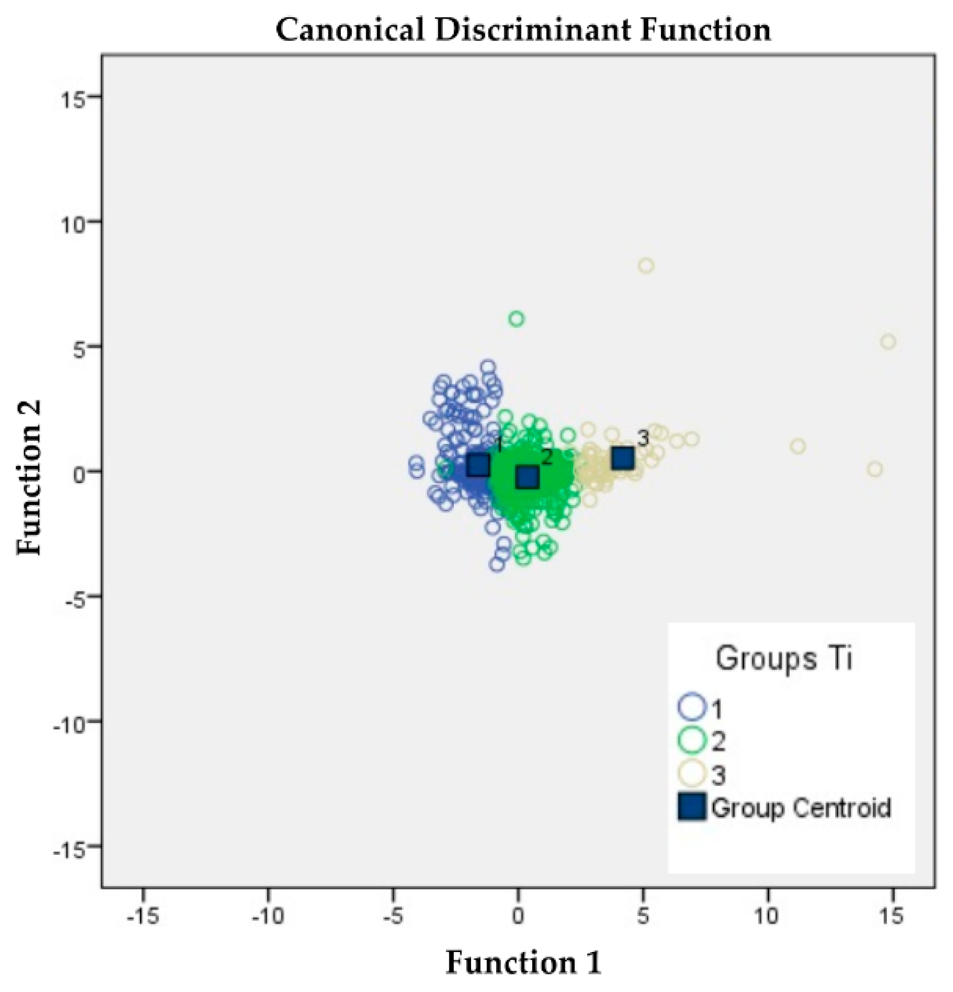
Minerals 10 00869 g012
Figure 13. Separated communities of titanium element using LDA method.
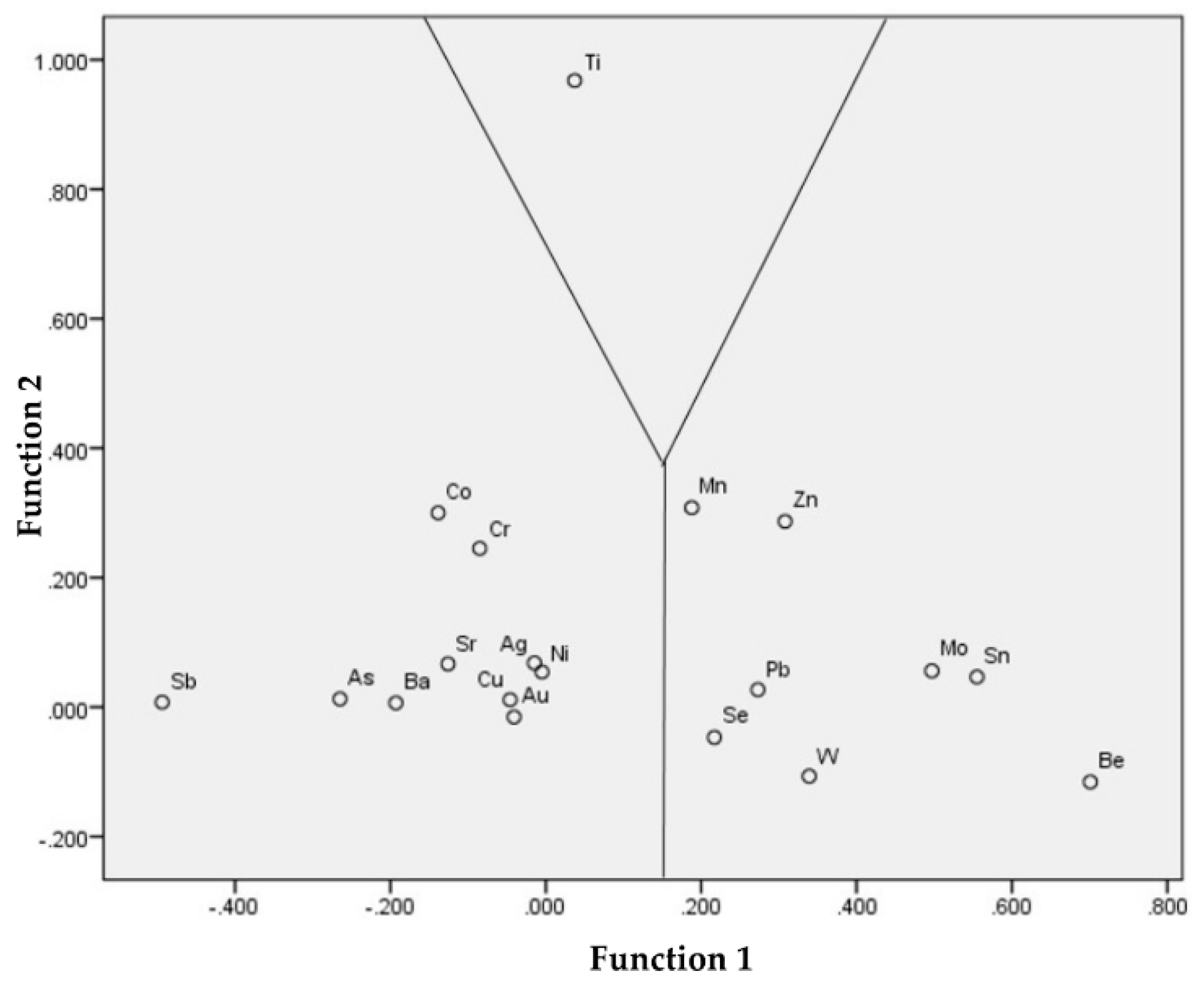
Minerals 10 00869 g013
Figure 14. Separated communities of titanium element with name of members.
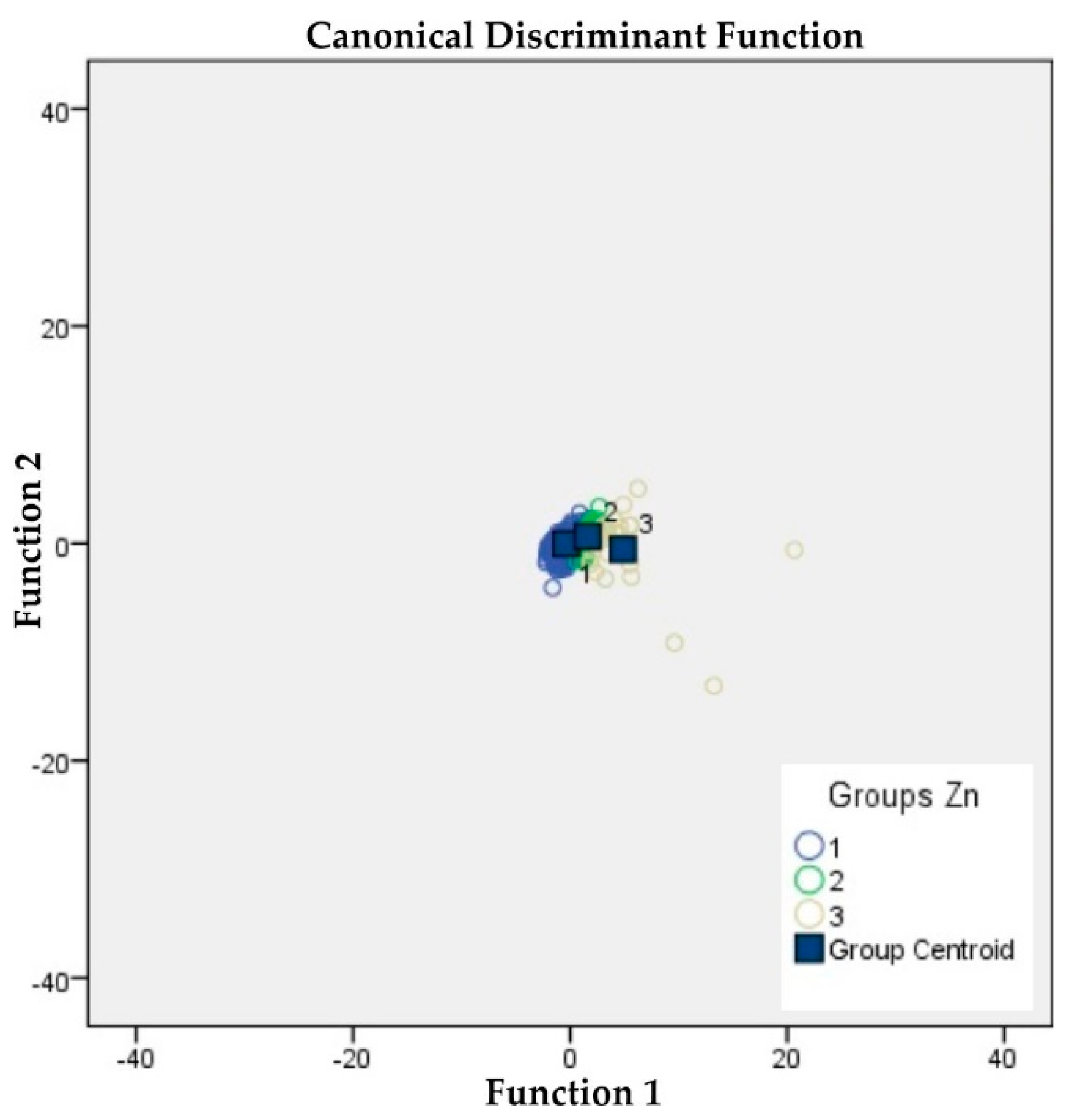
Minerals 10 00869 g014
Figure 15. Separated communities of zinc element using LDA method.
Minerals 10 00869 g015
Figure 16. Separated communities of zinc element with name of members.
Minerals 10 00869 g016
Figure 17. Map showing the distribution of Ti anomalous stream sediment samples.
Minerals 10 00869 g017
Figure 18. Anomalous samples of zinc element.
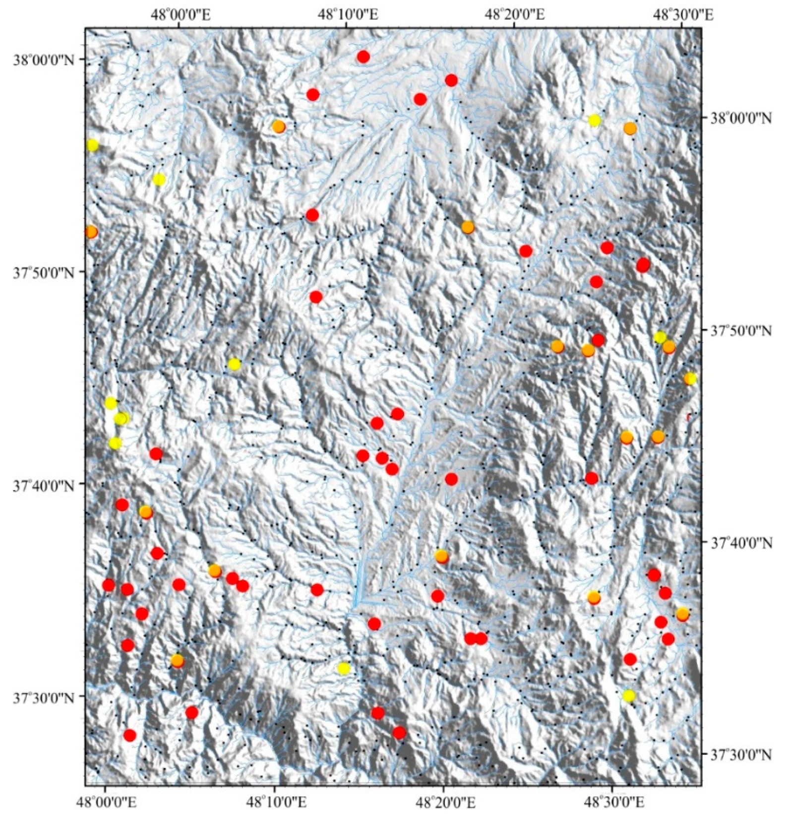
Minerals 10 00869 g018
Figure 19. Display zinc (yellow) and titanium (red) anomal points together.
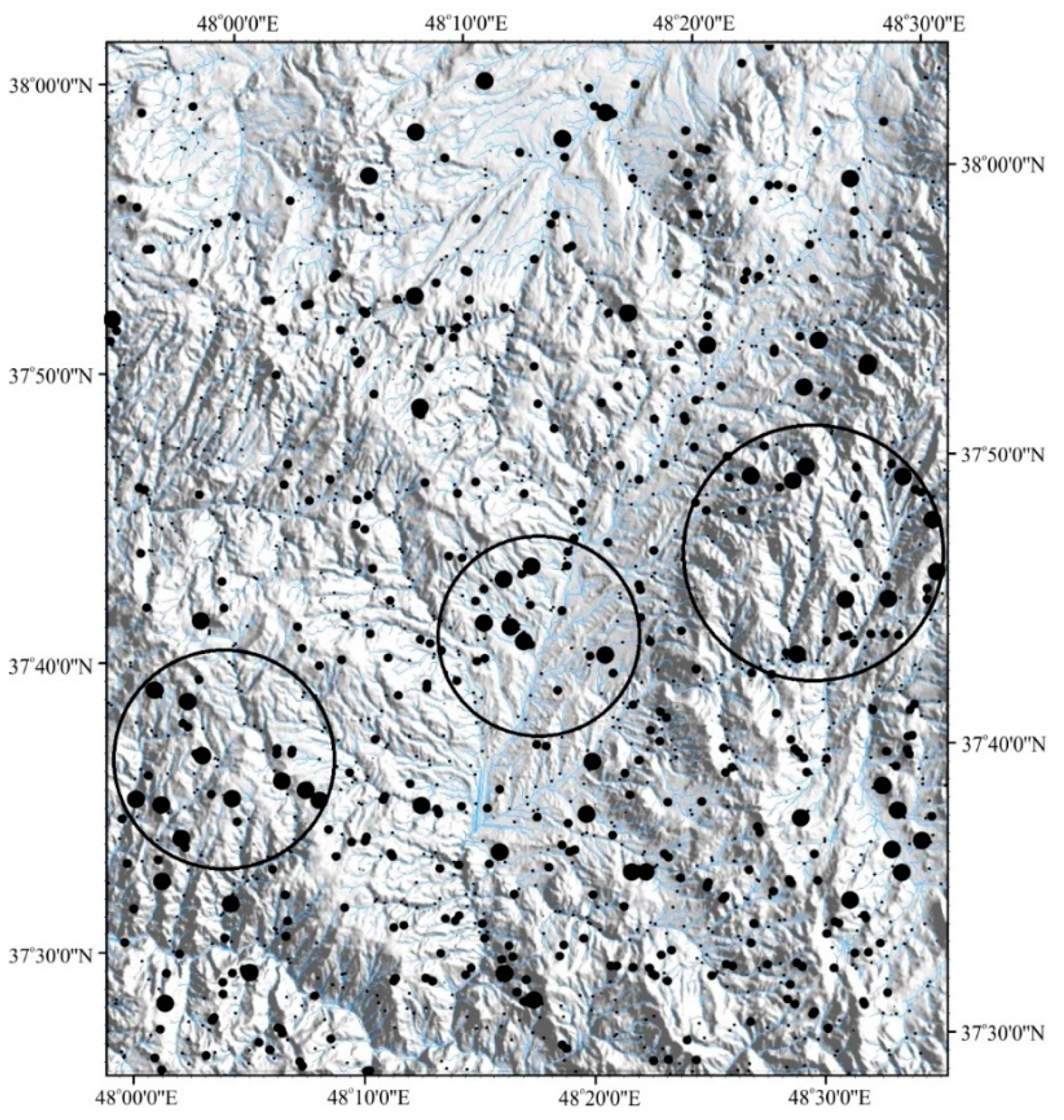
Minerals 10 00869 g019
Figure 20. Small to large titanium concentrations in the streams and determined anomalous areas.
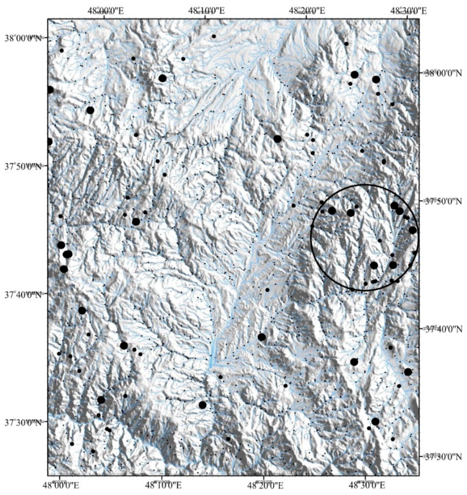
Minerals 10 00869 g020
Figure 21. Small to large zinc concentrations in the streams and determined anomalous areas.
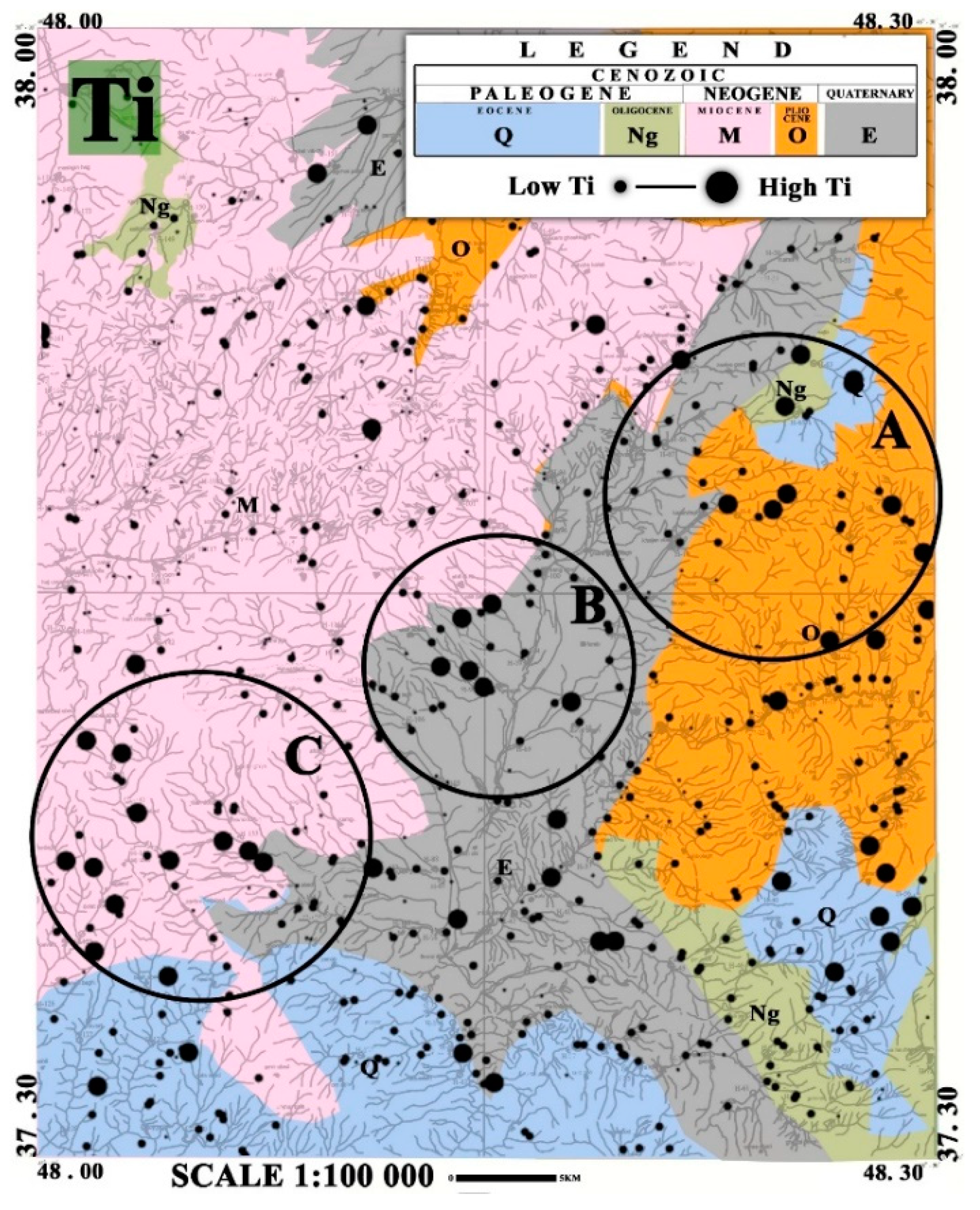
Minerals 10 00869 g021
Figure 22. Small to large titanium concentrations on the lithology map and determined anomalous areas.
Minerals 10 00869 g022
Figure 23. Small to large zinc concentrations on the lithology map and determined anomalous areas.
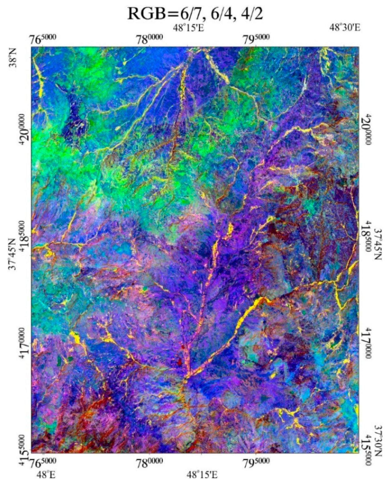
Minerals 10 00869 g023
Figure 24. Red, green, and blue colors (RGB) = 6/7, 6/4, 4/2 illuminates altered rocks as blue in image, yellow color lines are considered as vegetation.
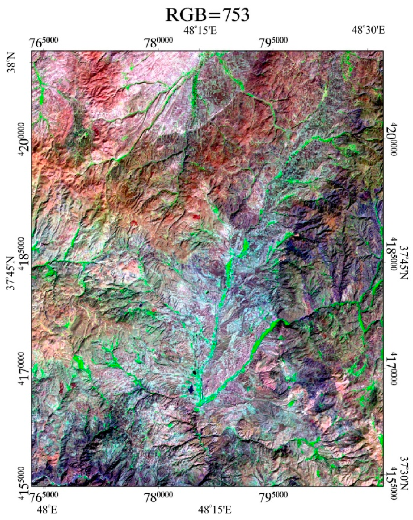
Minerals 10 00869 g024
Figure 25. RGB = 7, 5, 3 as derived from Operational land imager (OLI) data delineates altered rocks as bright white color; dark violet represents basalt, andesite, and thick bedded volcanic conglomerate rock units.
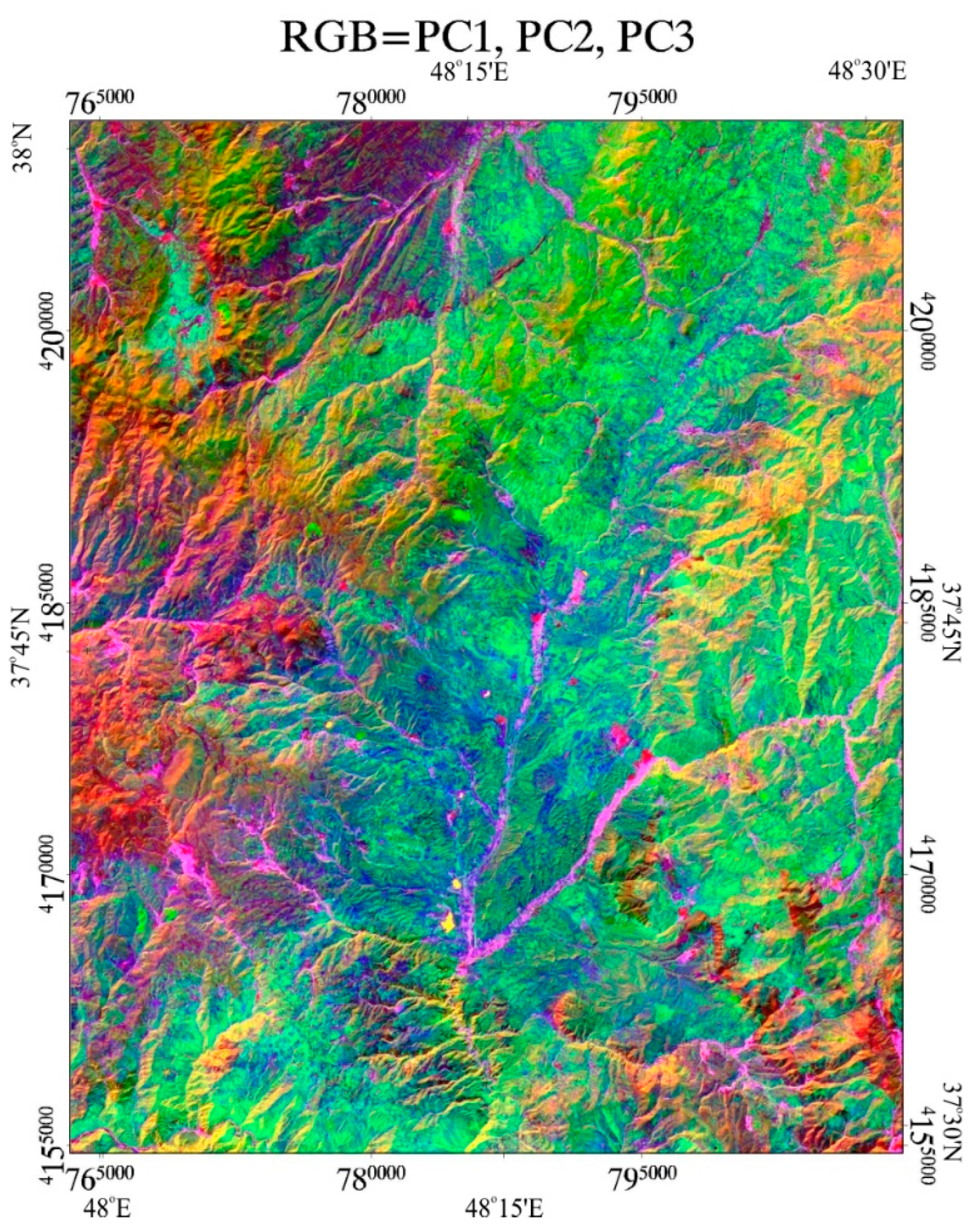
Minerals 10 00869 g025
Figure 26. RGB = PC1, PC2, and PC3, showing different rock classes in a variant range.
Minerals 10 00869 g026
Figure 27. 
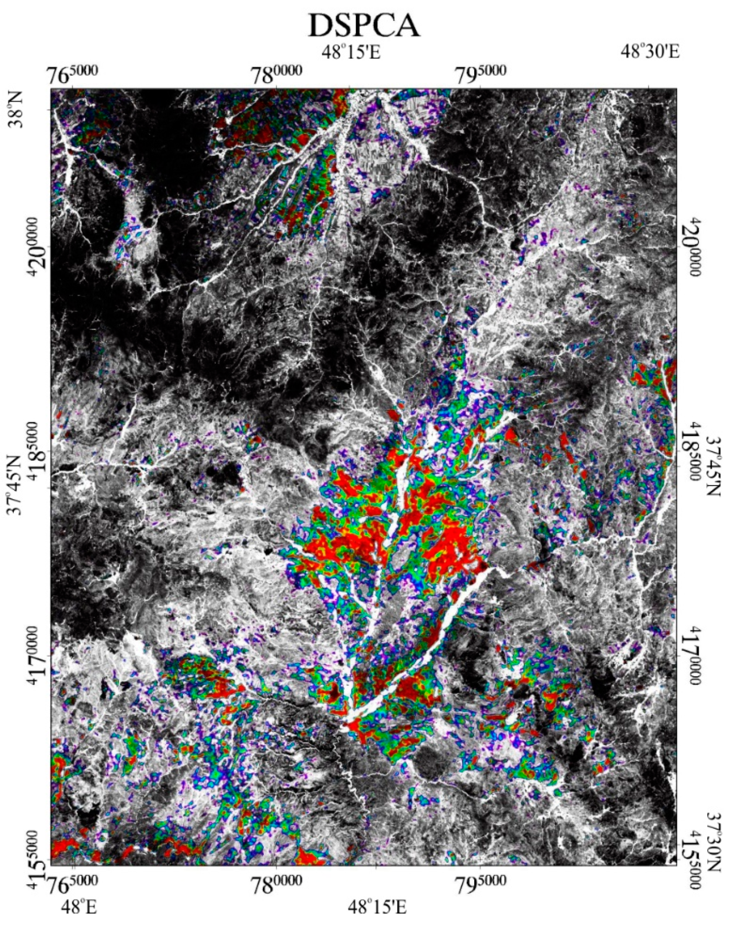
Alteration density map driven from band ratios and developed selective PCA (DSPCA) for detecting clay minerals in study area. Red color stands for extensive clay mineral overlay.
Minerals 10 00869 g027
Table 1. Element determined on the stream sediment samples (N = 714).
Elements
AgAlAsAuBaBBeBiBrCaCdCeCoCr
CsCuEuFFeGaGeHfHgInIrKLaLi
MgMnMoNaNbNdNiOsPPbPdPrPtRb
ReRuSSbScSeSiSnSrTaTeThTiTl
UVWYYbZnZr
Table 2. Analyzed elements after initial refinement.
Elements
AgAsAuBaBeCoCrCuMnMo
NiPbSbSeSnSrTiWZn
Table 3. Single-variable statistics parameters and anomalous limits for elements in drainage sediments.
ElementsMeanMedianModeMinMaxVarance (ppm)2SkewnessKurtosisStandard Deviation (ppm)CVAnomalous Limit (ppm)Anomal Priority
ppm
Ag00.150.130.034.800.07910.84147.20.2803140.170.17
As1510.854.90.50175250.784.3526.9215.84102.831 to 508
Au0000.000.020.0003.3418.900.001878.87--
Ba657661628169148042,519.10.195−0.005206.2131.41100 to 3000Suspicious
Be21.92.001141.493.9721.841.2255.526-
Co1816.65173.562.253.471.202.557.3140.621 to 40Suspicious
Cr7348401111007155.695.1841.8384.59116.525 to 10003
Cu8070112132221756.870.940.3241.9252.392 to 1005
Mn9899561000449316052,997.32.2713.03230.2123.288504
Mo21.901.50.138.63.4810.77202.71.8683.9926
Ni3527219210751.773.211.8127.4279.485 to 500Suspicious
Pb1615.415.15.956.220.462.3614.544.5228.632 to 200-
Sb21.30.80.225.35.683.6719.992.38113.535-
Se10.70.70.21.80.070.410.30.2638.45--
Sn21.51.40.88.20.552.9912.830.7441.3510-
Sr501490.546470103028,067.920.170.061167.5333.4450 to 10004
Ti568354405580194021,7002,938,2492.6016.791714.1330.1650001
W32.22.10.89.61.592.2046.591.2648.55--
Zn183.8200.4118102.346810.436.998.667.0033.9510 to 3002
Note: CV—Coefficient of variation.
Table 4. Correlation coefficients of the studied elements.
ElementsAgAsAuBaBeCoCrCuMnMoNiPbSbSeSnSrTiWZn
Ag1.000
As0.1281.000
Au0.0200.091.000
Ba0.0850.277−0.0911.000
Be0.1280.1820.10.211.000
Co−0.19−0.128−0.035−0.271−0.6461.000
Cr−0.089−0.064−0.073−0.327−0.5630.6781.000
Cu0.1710.0480.0190.516−0.0040.063−0.151.000
Mn−0.112−0.0610.015−0.092−0.0970.5260.387−0.0451.000
Mo0.2950.2410.0210.0810.523−0.381−0.1940.001−0.0461.000
Ni−0.083−0.138−0.013−0.442−0.4630.5810.822−0.2610.319−0.2481.000
Pb0.2480.3070.080.3450.689−0.518−0.3590.011−0.0820.506−0.3081.000
Sb0.2170.6550.0700.0150.058−0.1590.068−0.232−0.110.2830.0180.181.000
Se0.294−0.0770.028−0.2560.0330.0070.097−0.1610.10.2130.1330.0340.0481.000
Sn0.2560.2260.0680.0030.64−0.375−0.169−0.1880.0100.555−0.1810.6320.190.191.000
Sr−0.146−0.242−0.0880.403−0.2360.2530.0550.4290.102−0.1840.039−0.192−0.37−0.106−0.3361.000
Ti−0.0720.007−0.072−0.033−0.2590.5670.528−0.0130.524−0.0280.307−0.1530.051−0.0450.0390.1541.000
W0.1830.4090.1090.1890.697−0.569−0.382−0.105−0.1760.526−0.350.6310.3610.0780.638−0.263−0.2291.000
Zn0.065−0.0760.042−0.252−0.0500.420.411−0.0530.5340.0580.3180.064−0.0330.1860.207−0.0330.618−0.1611.000
Spearman Coloration method.
Table 5. Principal Components and their eigen values.
ElementsPC
123456
Ag0.011−0.0610.1340.1740.0970.827
As0.084−0.0060.084−0.0140.825−0.029
Au−0.1320.119−0.294−0.3950.3530.211
Ba−0.007−0.0810.838−0.1820.144−0.156
Be0.803−0.110−0.301−0.178−0.1470.011
Co−0.4850.338−0.1180.426−0.101−0.007
Cr−0.1770.306−0.1700.7840.0310.064
Cu−0.140−0.0380.750−0.113−0.0630.112
Mn−0.0130.851−0.0260.077−0.094-0.012
Mo0.6620.0040.0970.1510.0850.095
Ni−0.1820.178−0.2420.827−0.0430.088
Pb0.6880.1610.244−0.1690.3740.005
Sb0.147−0.003−0.091−0.0170.842−0.010
Se0.1700.095−0.302−0.128−0.1530.598
Sn0.8120.138−0.261−0.161−0.0470.054
Sr−0.4140.2280.557−0.050−0.277−0.095
Ti−0.0450.8050.0780.2060.017−0.023
W0.766−0.082−0.200−0.2030.224−0.004
Zn0.2210.826−0.067−0.0030.1520.071
Table 6. Anomalous values for titanium and zinc elements (ppm).
BackgroundAnomaly 1Anomaly 2Elements
50007800Upper 7800Ti
100120Upper 120Zn
Table 7. LDA titanium communities cross validation.
Titanium GroupsPredicted Group MembershipTotal
FirstSecondThird
CrossValidationCountFirst237140251
Second333691403
Third015960
PercentageFirst94.45.60100
Second8.291.60.2100
Third01.798.3100
Table 8. LDA zinc communities cross validation.
Zinc GroupsPredicted Group MembershipTotal
FirstSecondThird
Cross
Validation
CountFirst574530627
Second357060
Third012627
PercentageFirst91.58.50100
Second5950100
Third03.796.3100
Table 9. PCA eigenvector matrix for Kivi area.
Principal ComponentsSecond Band Fifth BandSixth BandSeventh Band
First PC+0.14+0.39+0.71+0.54
Second PC+0.28+0.78−0.32−0.36
Third PC+0.79−0.19−0.37+0.29
Forth PC−0.37+0.24−0.66+0.68

