Geometric Shape Characterisation Based on a Multi-Sweeping Paradigm

Abstract

The characterisation of geometric shapes produces their concise description and is, therefore, important for subsequent analyses, for example in Computer Vision, Machine Learning, or shape matching. A new method for extracting characterisation vectors of 2D geometric shapes is proposed in this paper. The shape of interest, embedded into a raster space, is swept several times by sweep-lines having different slopes. The interior shape’s points, being in the middle of its boundary and laying on the actual sweep-line, are identified at each stage of the sweeping process. The midpoints are then connected iteratively into chains. The chains are filtered, vectorised, and normalised. The obtained polylines from the vectorisation step are used to design the shape’s characterisation vector for further application-specific analyses. The proposed method was verified on numerous shapes, where single- and multi-threaded implementations were compared. Finally, characterisation vectors, among which some were rotated and scaled, were determined for these shapes. The proposed method demonstrated a good rotation- and scaling-invariant identification of equal shapes.

1. Introduction

Dealing with geometric data has become one of the main issues of many modern computer applications. There are countless solutions using geometric data in manufacturing, robotics, traffic, medicine, engineering, chemistry, cultural heritage, art, security, and defence. Unfortunately, answering questions about geometric shapes, which are treated easily by humans, frequently represents a considerable challenge to computers. Among such tasks are finding (almost) identical shapes, extracting those shapes that expose some kind of symmetry, finding the desired objects in point clouds obtained by remote sensing scanners, discovering pathological structures in medical images, or matching biometric data. Namely, the internal data structures storing the information about geometric shapes are designed with the main aim of how to represent the shapes in an unambiguous way [1,2] and do not support querying about the shapes’ characteristics directly.

In this paper, the shape characteristic corresponds to the description of the shape’s geometrical and/or topological properties in a countable way. We will refer to it as a characterisation in the continuation (terms such as attributes, properties, or features are also used [3]). This approach is based on geometric shapes’ local symmetries and the multi-sweeping paradigm [4] and works in 2D. The proposed method works in three steps:

• Initialisation, where a shape is inserted into a grid of equally sized cells;
• Processing, where the shape is swept several times with sweep-lines having different slopes; as a result of each sweep, the interior midpoints with respect to the shape boundary are determined and linked into the chains of midpoints;
• Finalisation, where the obtained chains are filtered, vectorised, and normalised. A shape’s characterisation vector is then formed from the polylines, which were obtained by the vectorisation.

The main benefits of this approach are the following:

• The obtained set of polylines enables the construction of various, application-specific characterisation vectors;
• It handles free-form shapes;
• It processes the shapes containing holes without any modifications in the algorithm;
• It can be parallelised.

The paper consists of five sections: Section 2 contains a summary of the previous works; Section 3 introduces the new shape characterisation approach; Section 4 presents the experimental results; Section 5 concludes the paper.

2. Related Works

The sweeping paradigm is explained first in this section. The shape characterisation methods, most similar to the introduced approach, are explained briefly after that.

2.1. Sweeping Paradigm

Sweeping, proposed by Shamos and Hoey [5], is an algorithmic paradigm used to solve various geometric problems. The idea is straightforward. Let s be a sweeping element (typically, a line in 2D or a plane in 3D), which glides continuously through the Euclidean space populated by geometric objects. When the geometric object of interest is hit by s, the sweeping element stops for a while, works out the considered problem locally, and updates an internal data structure. The stop is considered a sweep event, while the data structure a sweep status. In this way, the problem is solved behind s completely and unknown in front of it. When all the geometric objects have been passed by s, the sweep status contains the final solution of the considered problem. In practice, however, s does not glide continuously, but jumps from event to event. For this reason, the geometric objects should be sorted in regard to the movement of s before the sweeping is started. This is why s moves typically along one of the coordinate axes.

Many tasks have been solved efficiently by this strategy, such as, for example: computing the visibility on the terrain [6], establishing hierarchy among circles [7], constructing polygon trapezoidation [8], finding spatial clusters [9,10], constructing Delaunay triangulation [11,12] or a Voronoi diagram [13], determining the directional distance between points and shorelines [14], and many others.

2.2. Characterisation Methods and Skeletons

The characterisation of geometric shapes has attracted much research culminating in various reviews [15,16,17] and considered in books [18,19,20]. In general, the characterisation of shapes results either in a numerical value or in an alternative shape representation. The first group of methods parses the shape boundary and applies various transforms on it, while the second group stays in the space domain and produces another shape representation, from which a vector of values is derived (i.e., a characterisation vector). In the continuation, we review the latest ones briefly, among which the most-well-known is the medial axis transform or topological skeleton. There are, however, different terminologies in use [16]. However, for the purposes of this overview, we considered them the same and shall use the term skeleton in the continuation.

The skeleton (the concept was introduced by Blum [21]) is a set of all points being inside of the shape and having more than one closest point on its boundary. In this way, a reduced version of the shape is obtained, which contains enough information to reconstruct the shape. The skeleton captures the geometrical and topological characteristics of the shape and represents them internally with a graph, from which the characterisation information, such as the connectivity, lengths, directions, and widths, can be obtained directly. This information can then be used in the characterisation process. The main problem of the skeleton is its sensitivity to noise, as even a small change in the shape’s boundary can cause a considerable change in the graph’s topology. A different solution was proposed to mitigate this problem [22].

A simple polygon can be represented by a straight skeleton [23]. As the name suggests, it consists only of line segments in contrast to the topological skeleton, which may contain parabolic arcs. Its generalisation to general polygons was introduced shortly after that [24]. An algorithm for constructing an approximate straight skeleton using Steiner points was suggested in [25].

A scale axis transform, another type of skeleton, was proposed in [26]. It is defined by multiplicative scaling operations, with the aim to eliminate small local features of the shape. The points belonging to the skeleton are considered the centres of balls, touching at least two boundary points. By the gradual scaling of the shape, some balls become covered entirely by other balls. These covered balls are removed, and a hierarchical skeleton is obtained as a result. The skeleton is simplified most at the topmost level.

A $\beta$-skeleton was suggested in [27]. It is an undirected graph, defined on a set of points on the plane. The boundary points $p_i$ and $p_j$ are connected by an edge if there exists point q whose angle $\angle p_{i}q{p}_j$ is greater than the user-defined parameter $\beta$. The undirected graph is not always connected in this way.

Regardless of the skeleton type, it can be used for shape classifications, comparisons, and recognition. Various skeleton applications have been reported [28,29,30,31,32,33].

The most-recent studies in the field of shape characterisation heavily rely on neural networks and deep learning. Applications of these state-of-the-art techniques have been utilised successfully in numerous research domains, such as medicine [34,35], remote sensing [36], and physics [37]. Unfortunately, the downside of these methods is the requirement for large training sets in order to achieve high characterisation accuracy.

3. Materials and Methods

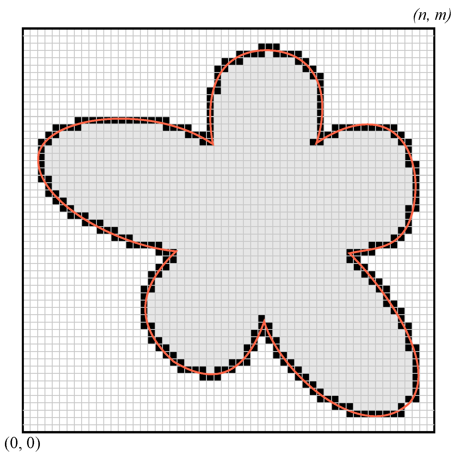
Let $\pi$ be a rasterised plane consisting of equally sized squared cells $c_{i,j}$, $0\le i<n$, $0\le j<m$, where n and m define the horizontal and vertical resolutions of $\pi$. Each cell $c_{i,j}$ is associated with an attribute $a_{i,j}\in \{I,B,E\}$, where I stands for interior, B for border, and E for exterior. Let $\mathcal{S}$ be a subset of $\pi$, such that $\mathcal{S}=\left\{c_{i,j}\right\}:a_{i,j}\in \{B,I\}$. In addition, let us introduce sweep-line $s\left(\alpha \right)$ with the slope $\alpha \in [0^{\circ },{180}^{\circ })$. $s\left(\alpha \right)$ investigates $\pi$ by gliding through it. The sweeping is repeated for different slopes $\alpha$; this is why the method is considered the Multi-Sweep Characterisation Algorithm (MSCA) in the continuation. It works in three main steps:

• Initialisation;
• Multi-sweeping;
• Finalisation.

These are discussed in the following subsections.

3.1. Initialisation

The MSCA accepts $\mathcal{S}$ either in a vector or a discrete form. The task of the initialisation is to unify these two possibilities for the unique processing. The bounding box $BBox\left(\mathcal{S}\right)=(x_{min},y_{min},x_{max},y_{max})$ is determined firstly in both cases, where $(x_{min},y_{min})$ and $(x_{max},y_{max})$ represent its left-bottom and right-upper corner, respectively. $BBox$ is then moved at the origin and becomes our rasterised plane $\pi$. If $\mathcal{S}$ is given in the discrete form (for example, by one of the known chain codes exposing four-connectivity [38,39,40,41]), the cell’s $size=1$, and the size of the bounding box is obtained as $n=x_{max}-x_{min}$ and $m=y_{max}-y_{min}$. Otherwise, when $\mathcal{S}$ is given in the vector form, suitable heuristics should be applied to determine the size and the number of cells n and m. $\mathcal{S}$ is rasterised by the four-connected rasteriser [42,43], and the shape’s boundary cells are obtained.

Having $\pi$ and the boundary cells determined, the interior cells are marked by setting $a_{i,j}=I$ by one of the shape-filling algorithms, while all the remaining cells are marked by setting $a_{i,j}=E$. Figure 1 shows the result of the initialisation for the demonstration shape, which has been given in the vector form at the input.

3.2. Multi-Sweeping

Because $\pi$ is discrete, some changes to the classical sweep-line paradigm (explained in Section 2.1) are needed in the MSCA:

• Sorting of geometric objects is not needed as the cells in $\pi$ are organised clearly;
• $\pi$ is not infinite, but bounded by its frontier cells, i.e., $c_{i,0}$, $c_{0,j}$, $c_{n-1,j}$, $c_{i,m-1}$, $0\le i<n$, $0\le j<m$;
• $s\left(\alpha \right)$ does not move from an event to an event, but advances through the consecutive frontier cells.

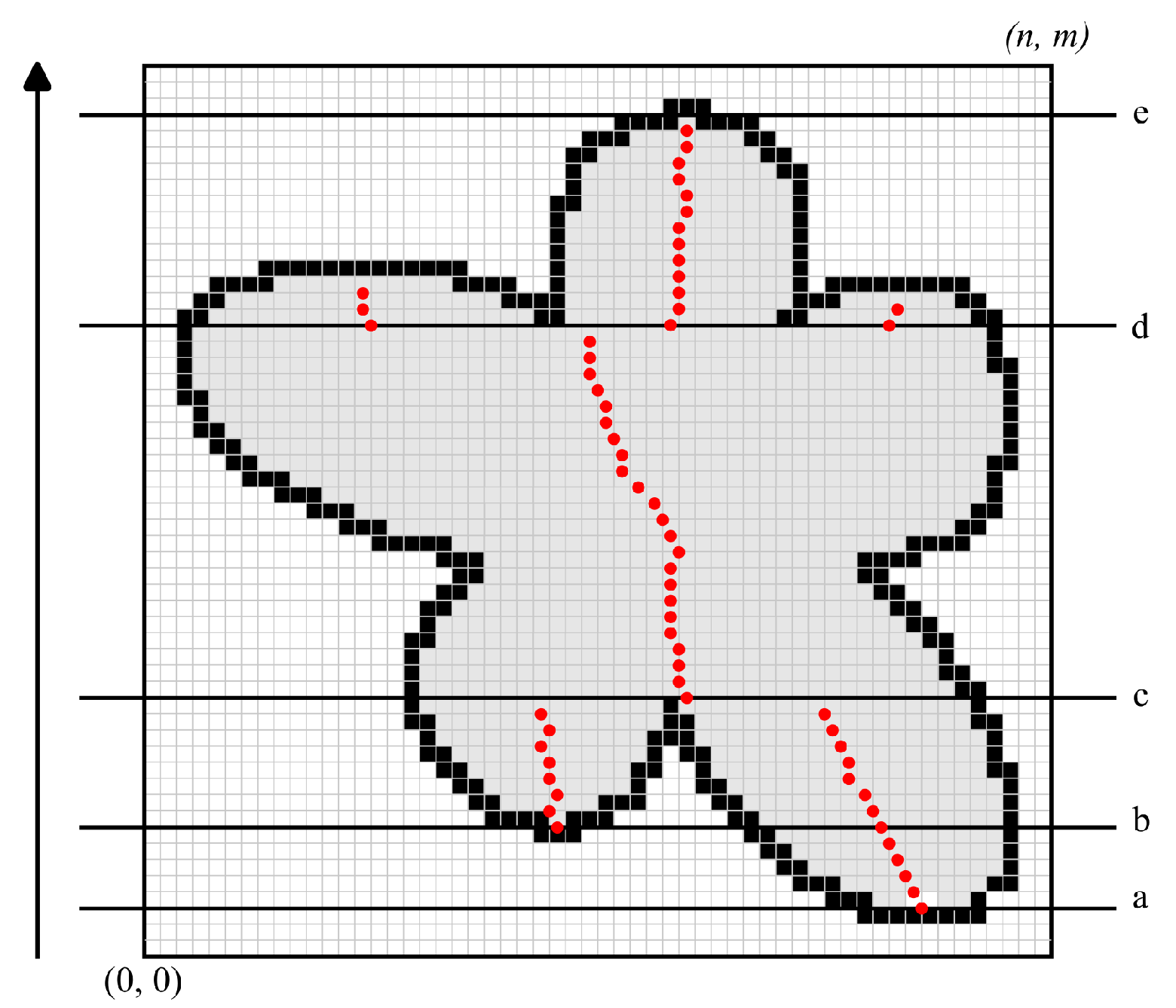
The multi-sweep part of the MSCA is explained by the pseudocode shown in Algorithm 1. An initialisation of variables is performed in Lines 8–10. The function in Line 14 (considered later in Algorithm 2) returns the endpoints $(x_1,y_1)$ and $(x_2,y_2)$ of the sweep-line segment $s\left(\alpha \right)$. The function also sets the flag, indicating whether the whole $\pi$ has been swept. If it has not, the intersections between $s\left(\alpha \right)$ and cells with $a_{i,j}=B$ are calculated by the function in Line 16. The midpoints $t_{i,j}$ between these intersections, which are inside $\mathcal{S}$, are calculated and returned in sequence $T=\langle t_{i,j}\rangle$ by the function in Line 17. They are appended to previously determined midpoints to form a set of chains $\mathcal{L}=\left\{L_i\right\}$, $L_i=\langle t_{i,j}\rangle$. The chains are controlled by two sweep-line events as follows:

• Chain $L_i$ is created when the local shape feature is met by $s\left(\alpha \right)$ (Sweep-lines a and b in Figure 2);
• Chain $L_i$ is terminated when the local shape feature is swept completely (Sweep-line c in Figure 2).

In this context, the local shape feature is any concave part of $\mathcal{S}$ (if $\mathcal{S}$ is convex, only one chain is obtained during each sweep). These two events can, however, appear simultaneously at any position of the actual $s\left(\alpha \right)$. For example, the chain (or more of them) can be terminated, and another one (or more of them) can be created at the same time (see Sweep-line c in Figure 2). The opposite case is shown for Sweep-line d in Figure 2, where one chain is terminated and three new chains are born. The obtained chains are stored in the sweep-line status $\mathcal{SLS}=\left\{L_i\right\}$. The whole process is repeated by increasing $\alpha$ in Line 22 by the user-defined parameter $step$. The MSCA terminates when $\alpha \ge {180}^{\circ }$. It returns terminated chains, stored in $\mathcal{SLS}$, for further processing.

It is obvious that the cardinality of $\mathcal{SLS}$ depends on the local shape’s features and the value of the parameter $step$. Although its actual value is not critical, some reasonable guidelines should be considered:

• Too small values result in many similar (or even equal) chains, which do not contribute additional information to the shape characterisation and slow down the whole process.
• Large values may cause some local feature to be missed if the filtering process, as described in Section 3.3, is applied.
• It is practical that $step$ is an integer divisor of ${180}^{\circ }$.

Various values of $step$ were evaluated in our experiments. However, the values for the parameter $step=i·{15}^{\circ },i=1,2,...,11$, yielded the best results.

Algorithm 1 The multi-sweep-line part of MSCA.

1: function Multi-sweep($step$, $size$, n, m, $\pi$) 2:                    ▹$step$: an increment of the sweep-line slope 3:                            ▹$size$: the size of the cell 4:                           ▹$n,m$: the resolution of $\pi$ 5:               ▹$\pi$: rasterised plane with embedded geometric shape $\mathcal{S}$ 6:                        ▹ returns list of resulting chains 7:      8:     $\mathcal{SLS}\leftarrow \varnothing$           ▹ Sweep-line status is empty at the beginning 9:     $\alpha$← 0${}^{\circ }$                     ▹ initial angle of sweep-line 10:   validSLCoordinates ← TRUE     ▹ Flag becomes FALSE when $\pi$ is swept 11:   repeat 12:         $\mathcal{L}\leftarrow \varnothing$                     ▹ set of chains is cleared 13:         repeat                       ▹ sweeping process 14:            validSLCoordinates ← GetSweepLineCoordinates $(\alpha ,size,n,m,x_1,y_1,x_2,y_2)$ 15:            if validSLCoordinates = TRUE then 16:                borderPixels ← SweepLineGridIntersections $(size,x_1,y_1,x_2,y_2,\pi )$ 17:                $T\leftarrow$ CalculateMidPoints(borderPixels) 18:                $\mathcal{L}\leftarrow$ ConcatenateMidPointsToChains $(T,\mathcal{L})$ 19:            end if 20:         until validSLCoordinates = FALSE 21:         $\mathcal{SLS}\leftarrow \mathcal{SLS}\cup \mathcal{L}$ 22:         $\alpha \leftarrow \alpha +step$ 23:     until $(\alpha \ge {180}^{\circ })$ 24:     return $\mathcal{SLS}$ 25: end function

The pseudocode in Algorithm 2 determines the endpoints of $s\left(\alpha \right)$. The function in Line 7 returns necessary frontier cells one by one until all of them are used. The returned frontier cells depend on $\alpha$ as shown in Figure 3, where these cells are coloured in blue. The frontier cell $(x_1,y_1)$, obtained by this function, is the first sweep-line coordinate. The second one is obtained by the function in Line 9. This function calculates the intersection point of the line passing through cell $(x_1,y_1)$ with slope $\alpha$ and pierces $BBox\left(\mathcal{S}\right)=(0,0,m,n)$.

Algorithm 2 Algorithm returns the sweep-line’s endpoints.

1: function GetSweepLineCoordinates($\alpha ,n,m,x_1,y_1,x_2,y_2$) 2:                             ▹$\alpha$: the sweep-line slope 3:                             ▹$n,m$: the resolution of $\pi$ 4:         ▹$x_1,y_1,x_2,y_2$; the endpoints of the sweep-line, returned by the function 5:      ▹ returns TRUE, if endpoints have been determined, and FALSE otherwise 6:      7:     $(\mathit{flag},x_1,y_1)$← GetNextStartingPoint $\left(\right)$ 8:     if flag = TRUE then 9:         $(x_2,y_2)\leftarrow$ GetSecondCoordinate $(\alpha ,n,m,x_1,y_1)$ 10:         return TRUE 11:     end if 12:     return FALSE 13: end function

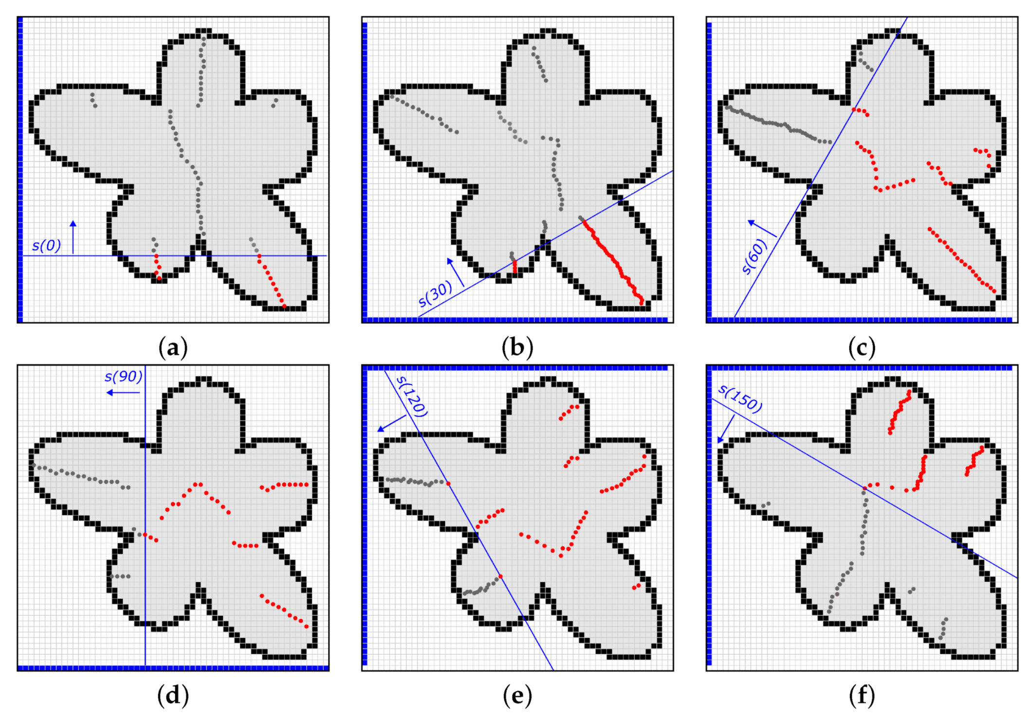
The results of multi-sweeping for slopes $\alpha =i·step,i=\{0,1,2,3,4,5\}$ and $step={30}^{\circ }$ are shown in Figure 3. Midpoints that have already been determined by $s\left(\alpha \right)$ are coloured in red. Meanwhile, midpoints that lie in front of $s\left(\alpha \right)$ and are yet to be discovered are plotted in grey.

3.3. Finalisation

Finalisation consists of three parts:

• Chain filtering;
• Chain vectorisation;
• Normalisation.

• Chain filtering: Different filtering methods can be designed; however, for demonstration purposes, the following two methods are proposed:

(a)

If $|L_i|\le \Delta$, then chain $L_i$ is removed from $\mathcal{SLS}$. $|L_i|$ denotes the number of points in $L_i$, while $\Delta$ is a threshold denoting the minimal number of midpoints in the chain. It may be determined by users or by heuristics. An example of such a heuristic used in the experiments presented in Section 4 is given in (1).

$$\begin{array}{c}\Delta =⌈\frac{max\{m,n\}}{20}⌉\end{array}$$

(1)

(b)

The average angle $\overline{\alpha }$ of lines is calculated, determined by the sequential pairs of midpoints $t_{x,y}\in L_i$. $L_i$ is accepted if $\overline{\alpha }$ is close to being perpendicular in regard to $\alpha$, i.e, if the heuristic, given in (2), is valid.

$${90}^{\circ }-0.25·step\le |\alpha -\overline{\alpha }|\le {90}^{\circ }+0.25·step.$$

(2)

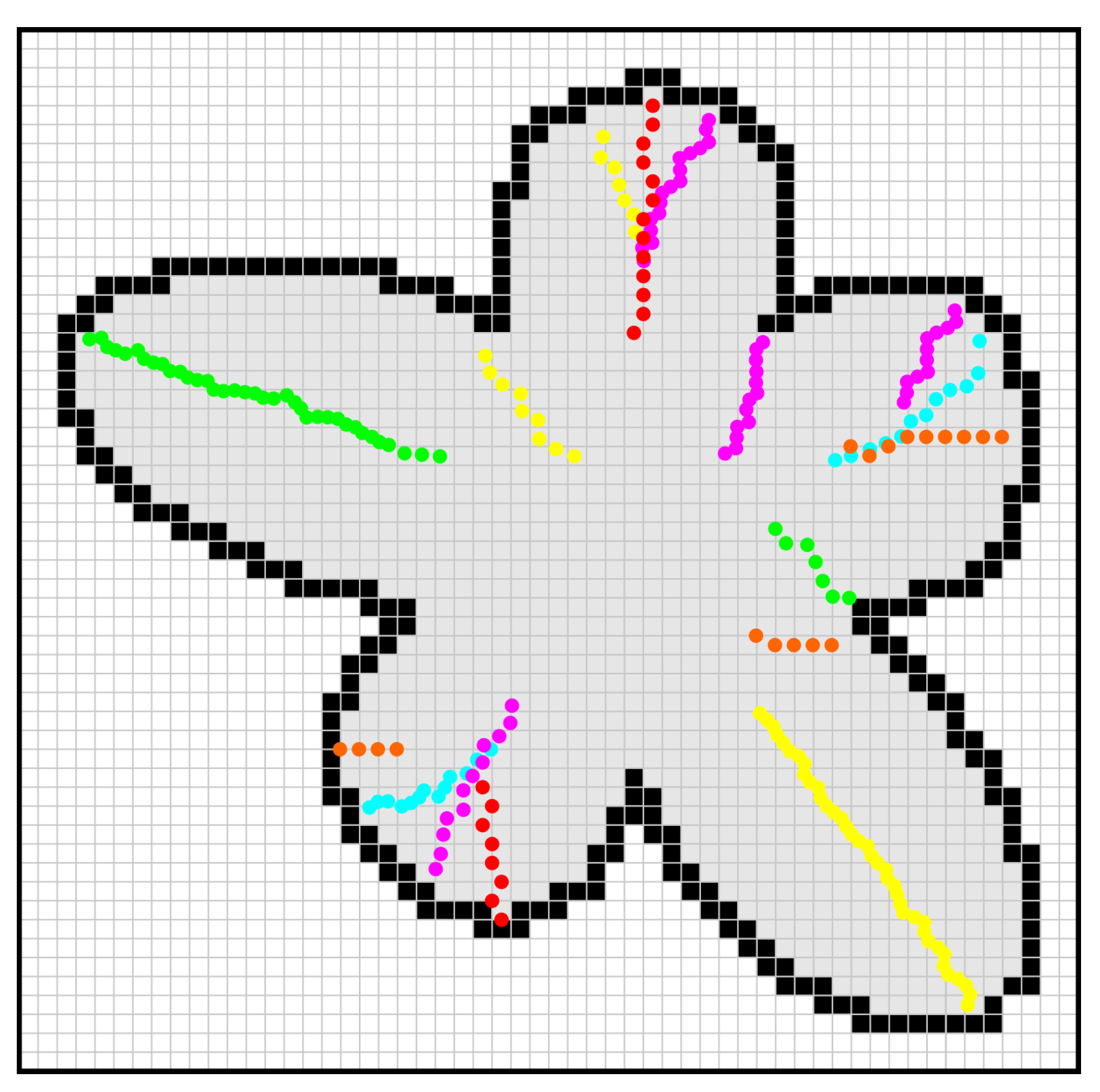
Figure 4 shows the remaining chains in $\mathcal{SLS}$ after filtering.

• Chain vectorisation: Round-off errors in the raster space $\pi$ are, unfortunately, unavoidable. Therefore, it is favourable to vectorise $L_i\in \mathcal{SLS}$ to minimise the effect of the round-off errors in the further characterisation process. The well-known Douglas–Peucker algorithm [44] was applied on $L_i\in \mathcal{SLS}$. The set of polylines $\mathcal{PL}=\left\{P{L}_i\right\}$ was obtained, which replaced $\mathcal{SLS}$ in the further steps of the algorithm.

• Normalisation: The normalisation is performed to make the characterisation of $\mathcal{S}$ insensitive to scaling or rotation. $BBox\left(\mathcal{S}\right)=BBox(0,0,n,m)$ is transformed into a normalised bounding box $BBo{x}^{*}\left(\mathcal{S}\right)$ according to (3).

  $$\begin{array}{c}q=max\{n,m\}\\ BBo{x}^{*}=\left\{0,0,\frac{n}{q},\frac{m}{q}\right\},\end{array}$$

  (3)

  and after that, $P{L}_i\in \mathcal{PL}$ are transformed similarly.

3.4. Time Complexity of the Algorithm

The MSCA operates in discrete space $\pi$, which consists of equally sized cells $c_{i,j}$, $0\le i<n$, $0\le j<m$. There are, altogether, $k=n\times m$ cells. The forming of $\pi$ with all k cells is performed in linear time $O\left(k\right)$. $\mathcal{S}$ is then embedded into $\pi$ to determine boundary cells, and after that, the remaining cells are classified as being either inside or outside of the shape. Each cell is visited only once, and therefore, the classification of all cells is performed in $O\left(k\right)$. It can, therefore, be concluded that the initialisation is performed in linear time $O\left(k\right)$.

The main part of the MSCA is multi-sweeping. Let us consider the whole sweep-line process for the given slope $\alpha$. Sweep-lines are sent through $m+n$ frontier cells. The first coordinate of each s is determined in this way, while the second is calculated in constant time $O\left(1\right)$ by determining the intersection of the bounding box and s. s is then rasterised, and the exact intersection points are calculated for cells with the attribute $a_{i,j}=B$. The number of boundary cells on s is considerably smaller than k, and as the calculation of the intersection points is performed in constant time, all intersection points on a sweep-line are obtained in $O\left(1\right)$. The midpoints $t_{i,j}$ between the obtained intersection points being inside $\mathcal{S}$ are calculated after that in $O\left(1\right)$. The sequence of midpoints T is obtained in this way. Midpoints from T are then concatenated to chains $\mathcal{L}$. However, as the number of chains is significantly smaller than k, this task is also terminated in $O\left(1\right)$. We have already stated that the count of all sweep-lines at an arbitrary angle $\alpha$ is at most $m+n\ll k$. However, all cells that form $\pi$ are visited during one sweep-line process, and therefore, the whole $\pi$ is swept in $O\left(k\right)$. The sweeping is repeated multiple times at various slopes. The number of slopes is considerably smaller than k; therefore, the time complexity of all different slopes remains $O\left(k\right)$.

Finalisation consists of three steps and operates only on obtained chains consisting of midpoints stored in $\mathcal{SLS}$. As the number of midpoints in $\mathcal{SLS}$ is significantly smaller than k, it can be accepted that the finalisation is performed in constant time $O\left(1\right)$. It can, therefore, be concluded that the proposed MSCA works in linear time $O\left(k\right)$, where k is the number of cells defining the raster space $\pi$.

4. Experiments

This section consists of two parts. The information about 12 testing shapes is given first, and the results of the MSCA are presented on them. The efficiency of the method was evaluated after that by measuring the CPU time spent on single- and multi-threaded implementations. In the second part, the MSCA was applied to find equal shapes, some of which were rotated and scaled. For this, a characterisation vector $V\left(\mathcal{S}\right)$ was constructed for each shape and compared against the characterisation vectors of the other shapes.

4.1. Demonstration of MSCA on Testing Shapes

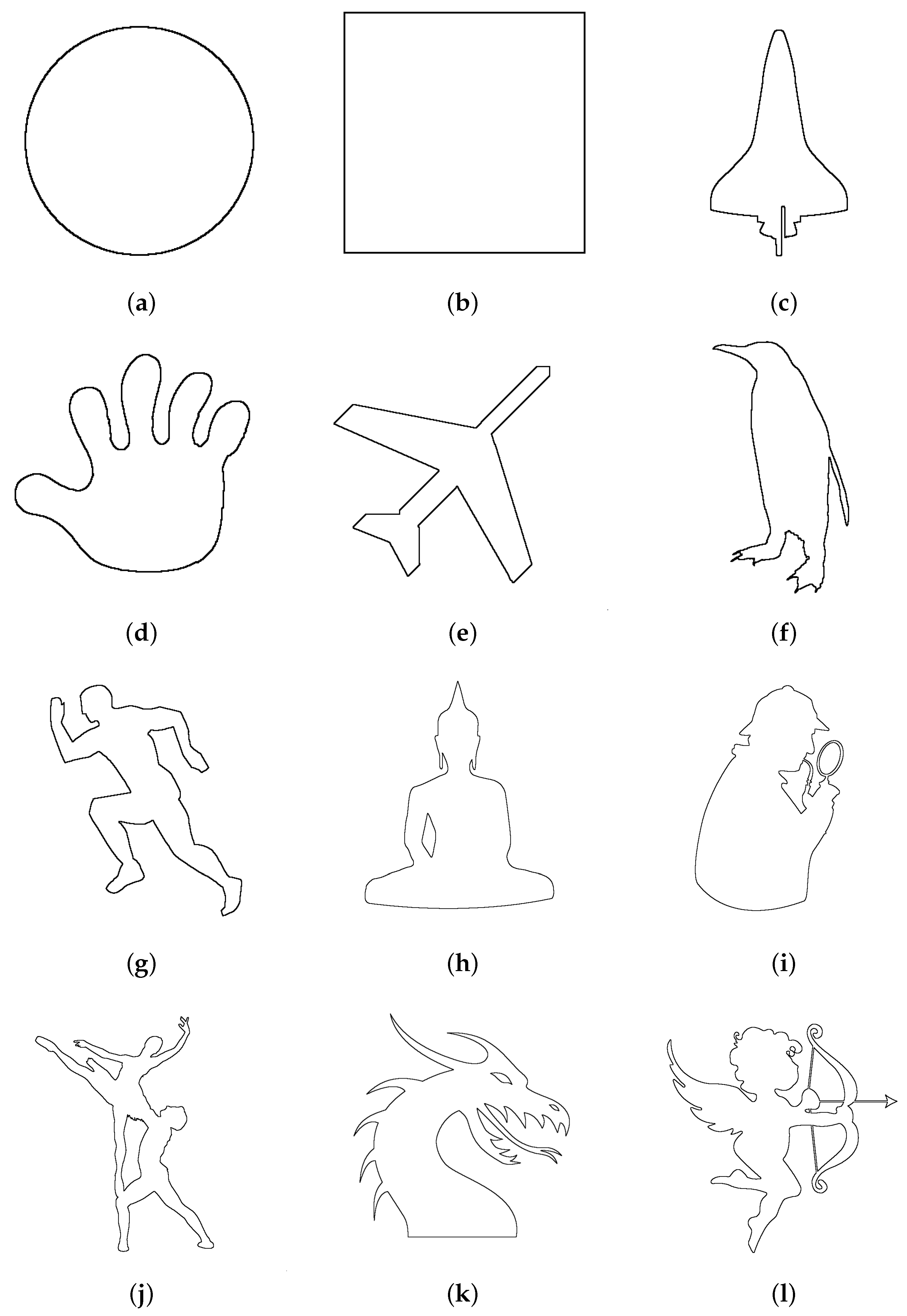
Twelve shapes, shown in Figure 5, were used in the experiments. Their borders were described by the Freeman chain code in eight directions [38]. The properties of these shapes and the number of detected chains are collected in

Table 1. Properties of $\mathcal{S}$.

$\mathcal{S}$	No. of ${\mathit{a}}_{\mathit{i},\mathit{j}}=\mathit{B}$	No. of. Holes	$\mathbf{BBox}\left(\mathcal{S}\right)$	No. of Chains
Circle	1068	0	327 × 327	12
Square	1068	0	327 × 327	12
Rocket	1232	0	343 × 412	26
Hand	1860	0	363 × 352	82
Airplane	2260	0	430 × 431	52
Penguin	1968	0	390 × 484	45
Runner	2896	0	471 × 508	56
Buddha	11,366	1	2648 × 2850	46
Detective	14,128	2	2440 × 2850	65
Ballet	16,712	1	2313 × 2575	117
Dragon	26,334	2	2807 × 2848	104
Cupid	25,160	4	2727 × 2721	157

.

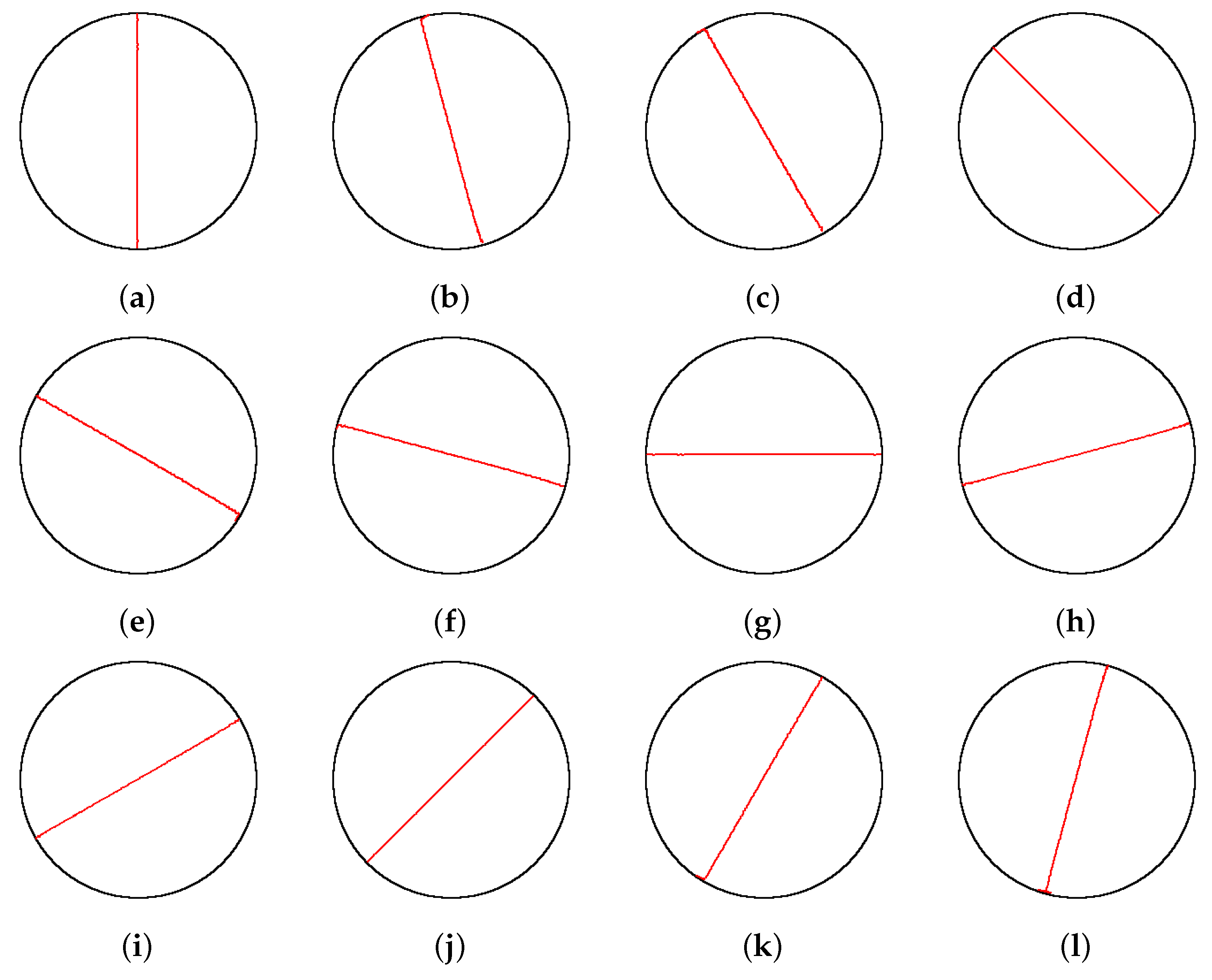
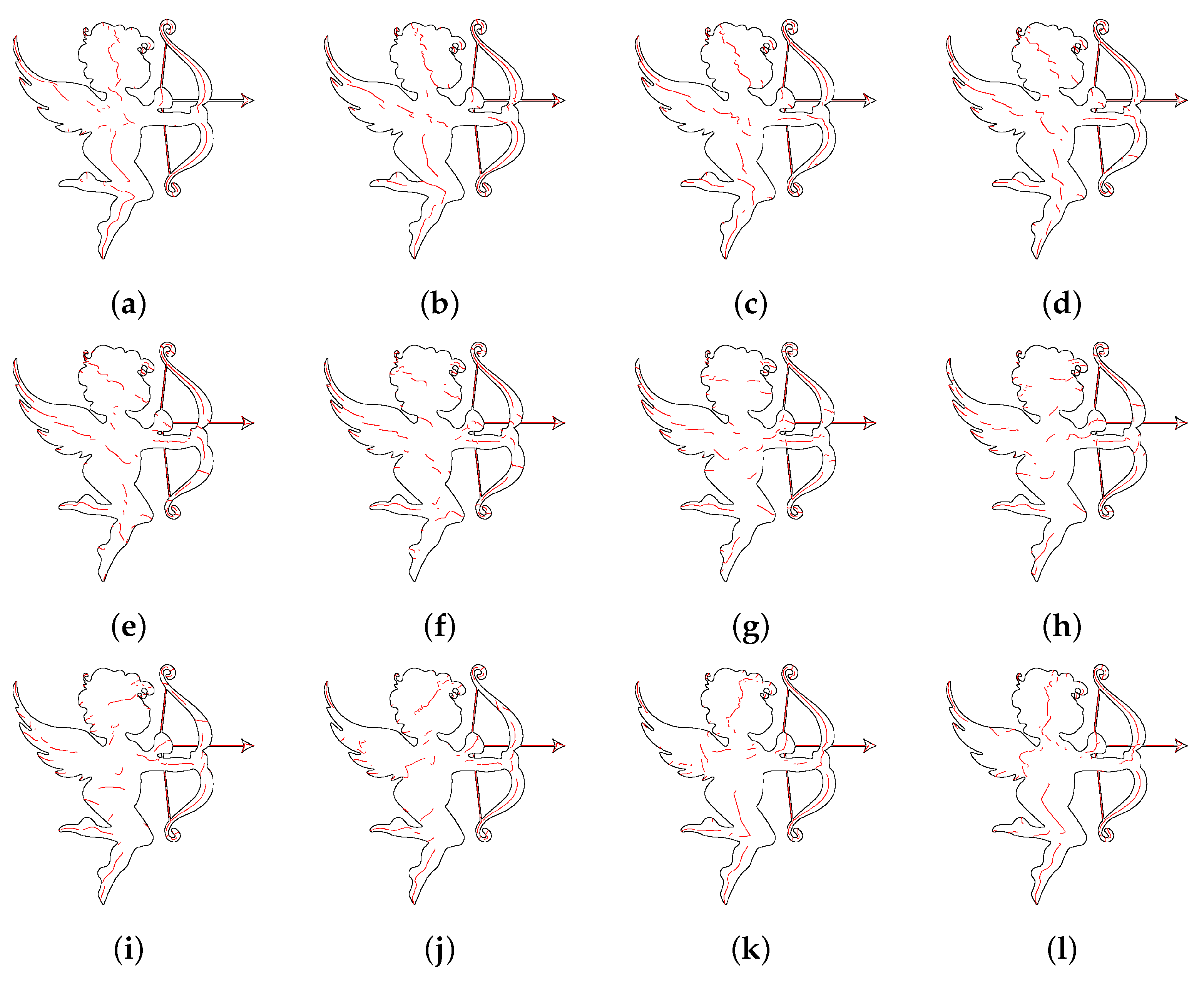
In the continuation, the results obtained by the MSCA for two shapes, Circle and Cupid, are shown in Figure 6 and Figure 7, respectively. Circle is the simplest shape, where the chains are in the form of straight lines. However, Cupid is a challenging shape containing holes and many concave parts. As can be seen, the MSCA handled both shapes successfully. It should be noted that the characterisation of these shapes can be performed equally successfully with other values of $step$ as far as the guidelines given in Section 3.2 are followed.

The CPU times spent by the MSCA are shown in

Table 2. CPU time of the MSCA spent for different shapes.

$\mathcal{S}$	Single-Threaded Time (s)	Multi-Threaded Time (s)
Circle	0.076	0.152
Square	0.081	0.183
Rocket	0.100	0.153
Hand	0.106	0.157
Airplane	0.132	0.205
Penguin	0.141	0.175
Runner	0.195	0.220
Buddha	3.508	1.798
Detective	4.311	1.712
Ballet	4.794	1.511
Dragon	9.297	2.630
Cupid	11.384	2.994

. A personal computer was used with an Intel i9-12900K CPU and 64 GB of DDR5 RAM running Windows 11. An MSVC compiler for C++, along with Microsoft Visual Studio 2022, were applied for development and compilation purposes. Two versions of the MSCA were implemented: the single- and the multi-threaded one using 12 threads. As shown, the multi-threaded implementation reduced the processing time considerably only for shapes with the larger $BBox$.

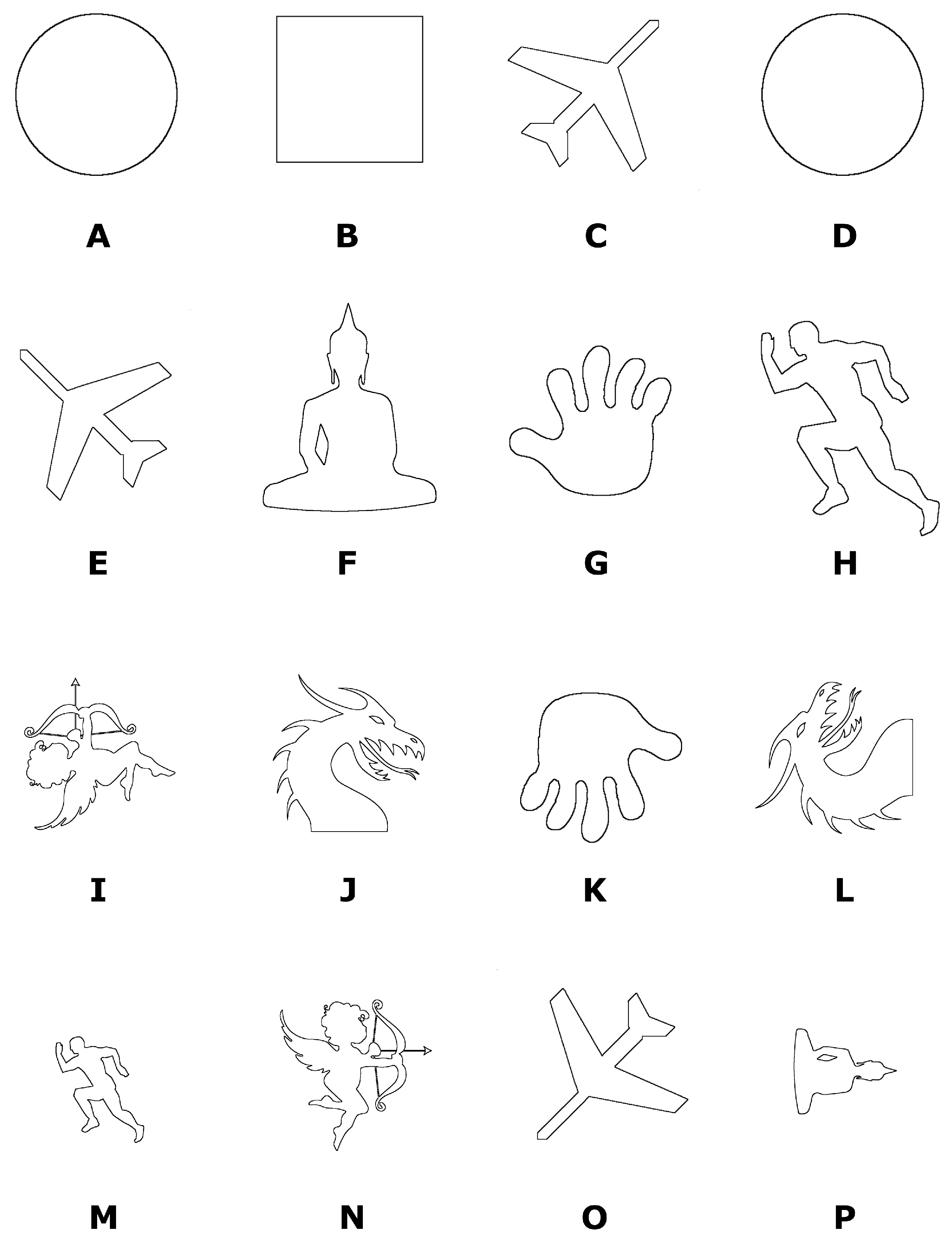
4.2. Recognition of Equal Objects

Arbitrary selected shapes from Figure 5 were used for this experiment. Some of them were rotated by a multiple of ${90}^{\circ }$, and some of them were enlarged by a factor of two, while the remaining shapes were just copied. The set of shapes obtained in this way is shown in Figure 8. The aim of the experiment was to find equal objects, regardless of whether they were rotated, scaled, or just duplicated. For this, characterisation vector $V^i\left(\mathcal{PL}\right)$ for shape ${\mathcal{S}}^i$ was constructed using the set of polylines $\mathcal{PL}$, produced by the MSCA. Various characteristics can, of course, be designed. $V^i\left(\mathcal{PL}\right)$ was formed in this experiment as follows:

• For each polyline $P{L}_k\in \mathcal{PL}$, $0\le k<\left|\mathcal{PL}\right|$, its length was calculated according to (4).

  $$\begin{array}{c}{V}_k^i={\displaystyle \sum _{l=0}^{l=|P{L}_k|-1}}D(P{L}_{k,l},P{L}_{k,l+1}),\mathrm{and}0\le k<\left|{\mathcal{PL}}^i\right|\end{array}$$

  (4)

  where D denotes the Euclidean distance between consecutive polyline points.
• Components $V_k^i$ of an individual vector $V^i$ were sorted after that in decreasing order.

Two shapes ${\mathcal{S}}^i$ and ${\mathcal{S}}^j$ are considered equal when:

• $|V^i|=|V^j|$, where $\left|\right|$ denotes the cardinality of vectors, and if this condition is true;
• $V_k^i\approx V_k^j$, $0\le k\le \lfloor 0.7\left|V^i\right|\rfloor$, where ≈ corresponds to a user-defined 5% tolerance.

This tolerance was determined experimentally as the best compromise between the ability of the algorithm to, despite the rounding errors, discriminate similar, yet different shapes (e.g., a circle or ellipse). The rounding errors, unfortunately, cannot be avoided during the sweep-line rasterisation process and geometric transformations of the shapes.

Table 3. Equality of the objects where letters refer to the shapes from Figure 8.

	A	B	C	D	E	F	G	H	I	J	K	L	M	N	O	P
A	– 1	$\times$ 2	$\times$	✓3	$\times$	$\times$	$\times$	$\times$	$\times$	$\times$	$\times$	$\times$	$\times$	$\times$	$\times$	$\times$
B	$\times$	–	$\times$	$\times$	$\times$	$\times$	$\times$	$\times$	$\times$	$\times$	$\times$	$\times$	$\times$	$\times$	$\times$	$\times$
C	$\times$	$\times$	–	$\times$	✓	$\times$	$\times$	$\times$	$\times$	$\times$	$\times$	$\times$	$\times$	$\times$	✓	$\times$
D	✓	$\times$	$\times$	–	$\times$	$\times$	$\times$	$\times$	$\times$	$\times$	$\times$	$\times$	$\times$	$\times$	$\times$	$\times$
E	$\times$	$\times$	✓	$\times$	–	$\times$	$\times$	$\times$	$\times$	$\times$	$\times$	$\times$	$\times$	$\times$	✓	$\times$
F	$\times$	$\times$	$\times$	$\times$	$\times$	–	$\times$	$\times$	$\times$	$\times$	$\times$	$\times$	$\times$	$\times$	$\times$	✓
G	$\times$	$\times$	$\times$	$\times$	$\times$	$\times$	–	$\times$	$\times$	$\times$	✓	$\times$	$\times$	$\times$	$\times$	$\times$
H	$\times$	$\times$	$\times$	$\times$	$\times$	$\times$	$\times$	–	$\times$	$\times$	$\times$	$\times$	✓	$\times$	$\times$	$\times$
I	$\times$	$\times$	$\times$	$\times$	$\times$	$\times$	$\times$	$\times$	–	$\times$	$\times$	$\times$	$\times$	✓	$\times$	$\times$
J	$\times$	$\times$	$\times$	$\times$	$\times$	$\times$	$\times$	$\times$	$\times$	–	$\times$	✓	$\times$	$\times$	$\times$	$\times$
K	$\times$	$\times$	$\times$	$\times$	$\times$	$\times$	✓	$\times$	$\times$	$\times$	–	$\times$	$\times$	$\times$	$\times$	$\times$
L	$\times$	$\times$	$\times$	$\times$	$\times$	$\times$	$\times$	$\times$	$\times$	✓	$\times$	–	$\times$	$\times$	$\times$	$\times$
M	$\times$	$\times$	$\times$	$\times$	$\times$	$\times$	$\times$	✓	$\times$	$\times$	$\times$	$\times$	–	$\times$	$\times$	$\times$
N	$\times$	$\times$	$\times$	$\times$	$\times$	$\times$	$\times$	$\times$	✓	$\times$	$\times$	$\times$	$\times$	–	$\times$	$\times$
O	$\times$	$\times$	✓	$\times$	✓	$\times$	$\times$	$\times$	$\times$	$\times$	$\times$	$\times$	$\times$	$\times$	–	$\times$
P	$\times$	$\times$	$\times$	$\times$	$\times$	✓	$\times$	$\times$	$\times$	$\times$	$\times$	$\times$	$\times$	$\times$	$\times$	–

¹ Not tested. ² Non-equality of a pair of shapes. ³ Equality of a pair of shapes.

reports the results of these experiments. The MSCA, with the proposed characterisation vector, found equal shapes successfully in all cases, regardless of their rotation and/or scaling. The proposed approach can also be adjusted to detect shapes that are not perfectly equal by softening the above two conditions. For example, the cardinalities ${\left|V\right|}^i$ and ${\left|V\right|}^j$ can be considered the same by allowing some variation and using a tolerance larger than 5%. However, these parameters should be determined by the user according to the specific application.

5. Conclusions

A new method for the characterisation of geometric shapes was presented in the paper. It was based on the sweeping paradigm, used frequently in traditional Computational Geometry. However, in this work, it was adapted for the raster space. The geometric shape was swept by following the frontier cells of the rasterised plane. The interior shape’s points, being in the middle of its boundary and laying on the sweep-line, were determined during each sweep step and connected in chains. Their construction was controlled by two sweep-line events. They used the local characteristics of the considered shape to determine the beginning and ending of each chain. The sweeping process was then repeated using different slopes of the sweep-line. The chains were filtered, vectorised, and normalised after that. As a result, a set of polylines was obtained, and various characterisation vectors can be extracted from it. The proposed approach utilised the local symmetry of the geometric shapes to recognise their eventual similarity, without the need to detect the symmetry explicitly. If the extraction of the local symmetrical features was the goal, the algorithm could also be generalised to produce such an output.

For the proof of concept, the method was implemented within the Multi-Sweep Characterisation Algorithm (MSCA). Its correctness and computational load were demonstrated by twelve testing shapes of different sizes and complexities (from the most simple circle to shapes with many concave parts and holes). Single- and multi-threaded implementations of the MSCA were tested, where the multi-threaded implementation was considerably faster for larger shapes. Finally, the results of the MSCA were used for finding equal shapes on the scene. A simple characterisation vector consisting of normalised polylines’ lengths was constructed for each shape. The proposed approach determined reliably equal shapes in all cases, regardless of their rotation or scaling.

The MSCA offers many new challenges for further research. Although its theoretical time complexity is linear in regard to the number of cells of the raster space $\pi$, it turned out to be rather slow for a large number of cells and the shapes containing holes and many concave shapes. Therefore, it would be worth investigating whether hierarchical spatial data structures, such as quadtree/octree or kd-trees, would accelerate the algorithm. For the proof of concept, the MSCA was implemented in 2D. Theoretically, it should also work in higher dimensions. Therefore, a 3D implementation will be performed in the future. The parameters of the MSCA were determined empirically in this research. It would be important to determine theoretically how to set these parameters optimally. New characterisation features can be constructed from the obtained chains, e.g., such that it measures the waviness of count junctions that occur when joining chains from sweep-lines with various angles. In addition, the result of the MSCA could be combined with other characterisation methods, for example with shape skeletons. Finally, the sweep-line itself could be replaced by different investigating elements; conics (i.e., a circle or circular arcs) should be the first choice.

References

- Mortenson, M.E. Geometric Modeling; Wileys: New York, NY, USA, 1985. [Google Scholar]
- Hoffmann, C.M. Geometric and Solid Modeling: An Introduction; Morgan Kaufmann Pub.: San Mateo, CA, USA, 1989. [Google Scholar]
- Liu, H.; Motoda, H. Feature Selection for Knowledge Discovery and Data Minimg; Kluwer Academic Publishers: New York, NY, USA, 1998. [Google Scholar]
- de Berg, M.; van Kreveld, M.; Overmars, M.; Schwarzkopf, O. Computational Geometry: Algorithms and Applications; Springer: Berlin, Germany, 1997. [Google Scholar]
- Shamos, M.I.; Hoey, D. Geometric intersection problems. In Proceedings of the 17th Annual Symposium on Foundations of Computer Science (SFCS 1976), Houston, TX, USA, 25–27 October 1976; pp. 208–215. [Google Scholar]
- Ferreira, C.R.; Andrade, M.V.A.; Magalhes, S.V.G.; Franklin, W.R.; Pena, G.C. A Parallel Sweep Line Algorithm for Visibility Computation. In Proceedings of the XIV GEOINFO, Campos do Jordão, Brazil, 24–27 November 2013; pp. 85–96. [Google Scholar]
- Kim, D.S.; Lee, B.; Sugihara, K. A sweep-line algorithm for the inclusion hierarchy among circles. Jpn. J. Ind. Appl. Math. 2006, 23, 127–138. [Google Scholar] [CrossRef]
- Žalik, B.; Jezernik, A.; Rizman Žalik, K. Polygon trapezoidation by sets of open trapezoids. Comput. Graph-UK 2003, 27, 791–800. [Google Scholar] [CrossRef]
- Rizman Žalik, K.; Žalik, B. A sweep-line algorithm for spatial clustering. Adv. Eng. Softw. 2009, 40, 445–451. [Google Scholar] [CrossRef]
- Lukač, N.; Žalik, B.; Rizman Žalik, K. Sweep-hyperplane clustering algorithm using dynamic model. Informatica 2014, 25, 564–580. [Google Scholar] [CrossRef] [Green Version]
- Domiter, V.; Žalik, B. Sweep-line algorithm for constrained Delaunay triangulation. Int. J. Geogr. Inf. Sci. 2008, 22, 449–462. [Google Scholar] [CrossRef]
- Žalik, B. An efficient sweep-line Delaunay triangulation algorithm. Comput. Aided Des. 2005, 37, 1027–1038. [Google Scholar] [CrossRef]
- Fortune, S. A sweepline algorithm for Voronoi diagrams. Algorithmica 1987, 2, 153–174. [Google Scholar] [CrossRef]
- Murtojärvi, M.; Leppänen, V.; Nevalainen, O.S. Determining directional distances between points and shorelines using sweep-line technique. Int. J. Geogr. Inf. Sci. 2009, 23, 355–368. [Google Scholar] [CrossRef]
- Pavlidis, T. A review of algorithms for shape analysis. Comput. Graph. Image Process. 1978, 7, 243–258. [Google Scholar] [CrossRef]
- Loncaric, S. A survey of shape analysis techniques. Pattern Recogn. 1998, 31, 983–1001. [Google Scholar] [CrossRef]
- Hossain, M.D.; Chen, D. Segmentation for Object-Based Image Analysis (OBIA) a review of algorithms and challenges from remote sensing perspective. ISPRS J. Photogramm. 2019, 150, 115–134. [Google Scholar] [CrossRef]
- Burger, W.; Burge, M.J. Principles of Digital Image Processing; Springer: London, UK, 2009. [Google Scholar]
- Solomon, C.; Brekon, T. Fundamentals of Digital Image Processing; Wiley-Blackwell: Chichester, UK, 2011. [Google Scholar]
- Gonzales, R.; Woods, R. Digital Image Processing; Pearson Prentice Hall: Upper Saddle River, NJ, USA, 2017. [Google Scholar]
- Blum, H. A Transformation for Extracting New Descriptors of Shape. In Models for the Perception of Speech and Visual Form; Wathen-Dunn, W., Ed.; MIT Press: Cambridge, MA, USA, 1967; pp. 362–380. [Google Scholar]
- Leborgne, A.; Mille, J.; Tougne, L. Extracting Noise-Resistant Skeleton on Digital Shapes for Graph Matching. In Advances in Visual Computing, Proceedings of the 10th International Symposium, ISVC 2014, Las Vegas, NV, USA, 8–10 December 2014; Bebis, G., Li, B., Yao, A., Liu, Y., Duan, Y., Lau, M., Khadka, R., Crisan, A., Chang, R., Eds.; Lecture Notes in Computer Science 8888 (Part II); Springer: Cham, Switzerland, 2014; pp. 293–302. [Google Scholar]
- Aichholzer, O.; Aurenhammer, F.; Alberts, D.; Gärtner, B. A novel type of skeleton for polygons. J. Univers. Comput. Sci. 1995, 1, 752–761. [Google Scholar]
- Aichholzer, O.; Aurenhammer, F. Straight skeletons for general polygonal figures in the plane. In Proceedings of the Annual International Conference on Computing and Combinatorics (COCOON’96), Hong Kong, 17–19 June 1996; Cai, J.-Y., Wong, C.K., Eds.; Lecture Notes in Computer Science 1090. Springer: Berlin/Heidelberg, Germany, 1996; pp. 117–126. [Google Scholar]
- Smogavec, G.; Žalik, B. A fast algorithm for constructing approximate medial axis of polygons, using Steiner points. Adv. Eng. Softw. 2012, 52, 1–9. [Google Scholar] [CrossRef]
- Giesen, J.; Miklos, B.; Pauly, M.; Wormser, C. The Scale Axis Transform. In Proceedings of the Twenty-Fifth Annual Symposium on Computational Geometry (SCG’09), Aarhus, Denmark, 8–10 June 2009; Hershberger, J., Fogel, E., Eds.; ACM: New York, NY, USA, 2009; pp. 106–116. [Google Scholar]
- Kirkpatrick, D.G.; Radke, J.D. A framework for computational morphology. In Computational Geometry, Machine Intelligence and Pattern Recognition; Toussaint, G.T., Ed.; Elsevier: Amsterdam, The Netherlands, 1985; Volume 2, pp. 217–248. [Google Scholar]
- Goh, W.-B. Strategies for shape matching using skeletons. Comput. Vis. Image Underst. 2008, 110, 326–345. [Google Scholar] [CrossRef] [Green Version]
- Ma, C.; Zhang, S.; Wang, A.; Qi, Y.; Chen, G. Skeleton-Based Dynamic Hand Gesture Recognition Using an Enhanced Network with One-Shot Learning. Appl. Sci. 2020, 10, 3680. [Google Scholar] [CrossRef]
- Liu, J.; Wang, G.; Duan, L.; Abdiyeva, K.; Kot, A.C. Skeleton-based Human Action Recognition with Global Context-Aware Attention LSTM Networks. IEEE Trans. Image Process. 2018, 27, 1586–1599. [Google Scholar] [CrossRef] [PubMed] [Green Version]
- Tasnim, N.; Islam, M.M.; Baek, J.-H. Deep Learning-Based Action Recognition Using 3D Skeleton Joints Information. Inventions 2020, 5, 49. [Google Scholar] [CrossRef]
- Papadopoulos, K.; Demisse, G.; Ghorbel, E.; Antunes, M.; Aouada, D.; Ottersten, B. Localized trajectories for 2D and 3D action recognition. Sensors 2019, 19, 3503. [Google Scholar] [CrossRef] [Green Version]
- Wang, C. Research on the Detection Method of Implicit Self Symmetry in a High-Level Semantic Model. Symmetry 2020, 12, 28. [Google Scholar] [CrossRef] [Green Version]
- Khanna, N.N.; Jamthikar, A.D.; Gupta, D.; Piga, M.; Saba, L.; Carcassi, C.; Giannopoulos, A.A.; Nicolaides, A.; Laird, J.R.; Suri, H.S.; et al. Rheumatoid arthritis: Atherosclerosis imaging and cardiovascular risk assessment using machine and deep learning-based tissue characterization. Curr. Atheroscler. Rep. 2019, 21, 7. [Google Scholar] [CrossRef] [PubMed]
- Dadoun, H.; Rousseau, A.L.; de Kerviler, E.; Correas, J.M.; Tissier, A.M.; Joujou, F.; Bodard, S.; Khezzane, K.; de Margerie-Mellon, C.; Delingette, H.; et al. Deep learning for the detection, localization, and characterization of focal liver lesions on abdominal US images. Radiol. Artif. Intell. 2022, 4, e210110. [Google Scholar] [CrossRef]
- Yan, X.; Ai, T.; Yang, M.; Yin, H. A graph convolutional neural network for classification of building patterns using spatial vector data. ISPRS J. Photogramm. Remote Sens. 2019, 150, 259–273. [Google Scholar] [CrossRef]
- Bisheh, M.N.; Wang, X.; Chang, S.I.; Lei, S.; Ma, J. Image-based characterization of laser scribing quality using transfer learning. J. Intell. Manuf. 2022, 34, 2307–2319. [Google Scholar] [CrossRef]
- Freeman, H. On the encoding of arbitrary geometric configurations. IRE Trans. Electron. Comput. 1961, EC10, 260–268. [Google Scholar] [CrossRef]
- Bribiesca, E. A new chain code. Pattern Recogn. 1999, 32, 235–251. [Google Scholar] [CrossRef]
- Sánchez-Cruz, H.; Rodríguez-Dagnino, R.M. Compressing bi-level images by means of a 3-bit chain code. Opt. Eng. 2005, 44, 1–8. [Google Scholar]
- Žalik, B.; Mongus, D.; Liu, Y.-K.; Lukač, N. Unsigned Manhattan chain code. J. Vis. Commun. Image Represent. 2016, 38, 186–194. [Google Scholar] [CrossRef]
- Cleary, J.C.; Wyvill, G. Analysis of an Algorithm for Fast Ray Tracing using Uniform Space Subdivision. Vis. Comput. 1988, 4, 65–83. [Google Scholar] [CrossRef]
- Žalik, B.; Clapworthy, G.; Oblonšek, Č. An Efficient Code-Based Voxel-Traversing Algorithm. Comput. Graph. Forum 1997, 16, 119–128. [Google Scholar] [CrossRef]
- Douglas, B.; Peucker, T. Algorithms for the reduction of the number of points required to represent a digitized line or its caricature. Cartographica 1973, 10, 112–122. [Google Scholar] [CrossRef] [Green Version]
Figure 1.
Result of the initialisation for the demonstration shape plotted in orange, where cells with are white, are black, while the grey cells indicate .
Figure 2.
Common sweep-line events (the arrow denotes the sweep-line moving direction, while the sequence of red dots belongs to the chains ; characteristic positions of sweep-line are marked with characters a–e).
Figure 3.
Results of multi-sweeping, when (a), (b), (c), (d), (e), and (f). The frontier cells utilised in the sweeping are coloured in blue.
Figure 4.
Chains after filtering, where the red points remain from , yellow from , green from , orange from , blue from , and purple from .
Figure 5.
Testing shapes: (a) Circle, (b) Square, (c) Rocket, (d) Hand, (e) Airplane, (f) Penguin, (g) Runner, (h) Buddha, (i) Detective, (j) Ballet, (k) Dragon, (l) Cupid.
Figure 6.
Chains produced by the MSCA for = when: (a) , (b) , (c) , (d) , (e) , (f) , (g) , (h) , (i) , (j) , (k) , and (l) .
Figure 7.
Chains obtained with the MSCA for = when: (a) , (b) , (c) , (d) , (e) , (f) , (g) , (h) , (i) , (j) , (k) , and (l) .
Figure 8.
Shapes used for detection of equality; the shapes are denoted by letters (A–P).