An Improved DCC Model Based on Large-Dimensional Covariance Matrices Estimation and Its Applications

Abstract

The covariance matrix estimation plays an important role in portfolio optimization and risk management. It is well-known that portfolio is essentially a convex quadratic programming problem, which is also a special case of symmetric cone optimization. Accurate covariance matrix estimation will lead to more reasonable asset weight allocation. However, some existing methods do not consider the influence of time-varying factor on the covariance matrix estimations. To remedy this, in this article, we propose an improved dynamic conditional correlation model (DCC) by using nonconvex optimization model under smoothly clipped absolute deviation and hard-threshold penalty functions. We first construct a nonconvex optimization model to obtain the optimal covariance matrix estimation, and then we use this covariance matrix estimation to replace the unconditional covariance matrix in the DCC model. The result shows that the loss of the proposed estimator is smaller than other variants of the DCC model in numerical experiments. Finally, we apply our proposed model to the classic Markowitz portfolio. The results show that the improved dynamic conditional correlation model performs better than the current DCC models.

1. Introduction

In the era of information explosion, high-dimensional data is used widely in various fields such as biology, medicine, finance, signal processing, etc. [1,2,3,4]. High-dimensional data bring challenges to traditional statistical and computational methods. For instance, in the financial area, financial data are usually characterized by large dimension, non-normality and positive correlation so that the covariance matrix estimation becomes a popular issue [5,6,7].

Recently, the estimation and modeling of large-dimensional sparse covariance matrix have attracted extensive attention of scholars. A key point in the literature is to assume that the target matrix is sparse; see, for instance [2,8]. Furthermore, a common method is to construct a convex optimization model by using norm penalty [9,10,11,12]. Moreover, to reduce the estimation bias, Fan et al. [13,14] constructed nonconvex optimization model to estimate the sparse precision matrix and studied their theoretical properties.

It is well-known that a covariance matrix or correlation matrix is affected by the market information. Thus, Engle [15] proposed the DCC model based on constant correlation model [16] and GARCH model [17]. However, the performance of the DCC model is not good because of the dimension and the noise in large dimensional data. To reduce the dimension of data and remove the noise, Engle et al. [5] applied the nonlinear shrinkage method [18] to the DCC model on the aspects of eigenvalues, which optimized the performance of the DCC model. Furthermore, De Nard et al. [19] applied this model to intraday data to predict dynamic conditional covariance matrix. Since the DCC model needs to normalize the conditional correlation matrix to obtain the dynamic conditional covariance matrix, it leads to compromising the model fit. From this perspective, Jarjour et al. [20] proposed dynamic conditional angular correlation model based on the DCC model and Tse and Tsui [21] proposed a time-varying conditional correlation model, and an empirical research showed that the dynamic conditional angular correlation model outperforms in the DCC model for small sample in portfolio construction. More information on the applications of the DCC model in portfolio can be refered to [6,19,20,22].

In addition, Wen et al. [23] proposed a class of positive-definite covariance estimators to realize sparsity and positive definiteness by using generalized nonconvex penalties. However, the covariance matrix estimation with nonconvex function performs worse in high noise. In order to resolve this problem, Zhang et al. [24] constructed a optimal convex combination of the linear shrinkage estimation and the rotation-invariant estimator to remove the noise under the Frobenius norm. Although the new estimator can significantly remove the sampling noise, it does not consider the variance, and covariance varies with time.

Motivated by [5,23,24] and a special case of symmetric cone optimization, in this paper, we consider the following factors:

• We propose a new large covariance matrix estimator to realize the sparsity and positive-definiteness by constructing a nonconvex optimization model with smoothly clipped absolute deviation (SCAD) and hard threshold penalty functions based on the rotation-invariant estimator.
• To improve the performance of the DCC model, we use the new covariance matrix estimator to replace the unconditional covariance matrix in the DCC model.
• We show that the improved DCC model has a smaller loss and lower out-of-sample risk in portfolio optimization model.

The outline of this article is as follows: Section 2 describes the preliminary work. Section 3 introduced the proposed estimator. Section 4 implements the numerical simulation and application. Section 5 makes a discussion and Section 6 gives a conclusion.

2. Preliminary Work

2.1. Covariance Matrix Estimation Based on Convex Combination

In random matrix theory, the eigenvalues inside and outside the boundary of Mar$\breve{c}$enko and Pastur law generate noise so that they affect the estimation of covariance matrix. In order to deal with the noise caused by these two types of eigenvalues simultaneously, Zhang et al. [24] used a optimal convex combination of the shrinkage transformation and the rotation invariant estimator to remove noisy correlations. In what follows, we briefly introduce the model.

Let $\Sigma$ be a true covariance matrix, Zhang et al. [24] constructed the following convex optimization model, i.e.,

$$\underset{\theta ,\varphi }{\min }\left|\right|\Sigma -{\Sigma }_{est}{\left|\right|}_F^2$$

(1)

$$\mathrm{s}.\mathrm{t}.\left\{\begin{array}{c}{\Sigma }_{\mathrm{est}}=\varphi (\theta {\Sigma }_{\mathrm{F}}+(1-\theta ){\Sigma }_{\mathrm{RIE}})+(1-\varphi ){\Sigma }_{\mathrm{S}},\hfill \\ 0\le \theta \le 1,0\le \varphi \le 1.\hfill \end{array}\right.$$

where ${\Sigma }_F$, ${\Sigma }_{RIE}$, ${\Sigma }_S$ and ${\left|\right|.\left|\right|}_F$ denoted the shrinkage target matrix [7], rotation invariant estimator [25] and the sample covariance matrix [5], and Frobenius norm, respectively. Now, let ${\theta }^{*}$ and ${\varphi }^{*}$ be the optimal parameters. It follows from (1) that the optimal covariance matrix estimation under the Frobenius norm is given by

$${\Sigma }^{*}={\varphi }^{*}({\theta }^{*}{\Sigma }_F+(1-{\theta }^{*}){\Sigma }_{RIE})+(1-{\varphi }^{*}){\Sigma }_S$$

This model effectively eliminates the sample noise generated by the eigenvalues inside and outside the boundary of Mar$\breve{c}$enko and Pastur law, so that it can improve the estimation efficiency of the covariance matrix. The more details refer to [24].

2.2. Classical DCC Model

Although the positive-definite estimator with the SCAD penalty function is of a good theoretical properties, in financial research, the covariance matrix or correlation matrix changes over market information and is affected by large dimensions and noise. Therefore, studying the conditional covariance matrix is of theoretical and practical significance. Engle [15] proposed the DCC model below, which takes into account the impact of the past market information on the correlation matrix or covariance matrix.

Let $r_{i,t}$ denote asset return series i at date t, $r_t:=(r_{1,t},\dots ,r_{N,t})$, and $r_t$ obeys standardized normal distribution. Then,

$$H_t=D_t{R}_t{D}_t,$$

(2)

$$r_t|\varphi \sim N(0,D_t{R}_t{D}_t),$$

$$d_{i,t}^2={\omega }_i+{\alpha }_i{r}_{i,t-1}^2+{\beta }_i{d}_{i,t-1}^2,$$

(3)

$$D_t^2=diag\left\{{\omega }_i\right\}+diag\left\{{\alpha }_i\right\}{r}_{t-1}^{\prime }{r}_{t-1}+diag\left\{{\beta }_i\right\}{D}_{t-1}^2,$$

(4)

$$R_t=diag{\left\{Q_t\right\}}^{-1}{Q}_{t}diag{\left\{Q_t\right\}}^{-1},$$

(5)

where $d_{i,t}=\mathrm{var}\left(r_{i,t}\right|F_{t-1})$ is the conditional variance of ith asset at date t, $D_t$ denotes the N dimensions diagonal matrix with diagonal entries $d_{i,t}$ ($i=1,\dots ,N$), $R_t$ denoted the dynamic conditional correlation matrix and dynamic conditional covariance matrix $Q_t$ is defined by the following way:

For arbitrary $\alpha ,\beta$ and $\alpha +\beta \le 1$,

$$Q_t=(1-\alpha -\beta )\overline{S}+\alpha q_{t-1}^{\prime }{q}_{t-1}+\beta Q_{t-1}.$$

(6)

where $\overline{S}$ is the unconditional covariance matrix of $q_t=D_t^{-1}{r}_t$, which denotes the standard return at date t, and $q_t\sim N(0,I_N)$.

3. An Improved DCC Model Based on Nonconvex Combination

Since most of off-diagonal entries of the covariance matrix are close to zero in numerical experiments and empirical studies, we propose the constrained covariance matrix estimation to achieve sparsity and positive-definiteness simultaneously, which solves the following problem

$$\underset{\Sigma }{\min }\left|\right|\Sigma -{\Sigma }^{*}{\left|\right|}_F^2+g_{\lambda }(\Sigma ),$$

(7)

$$\mathrm{s}.\mathrm{t}.\left\{\begin{array}{c}diag(\Sigma )=I_d,\hfill \\ \Sigma \ge ϵI_d,\hfill \\ ϵ>0.\hfill \end{array}\right.$$

where $g_{\lambda }(\Sigma )$ is the penalty function and $\lambda$ is the penalty parameter. In [9,10,11], the alternating direction method (ADM) and the augmented Lagrangian method (ALM) algorithm are used to solve the nonconvex optimization model. Wen et al. [23] pointed out that the ADM algorithm is more effective for the optimization model with nonconvex penalty function.

There are many penalty functions in existing literatures. For instance, Fan et al. [13] first proposed the SCAD penalty function, i.e.,

$$p_{\lambda }^{scad}\left(y\right)=\left\{\begin{array}{cc}\lambda \left|y\right|,\hfill & 0\le \left|y\right|<\lambda ,\hfill \\ 2b\lambda \left|y\right|-y^2-{\lambda }^2,\hfill & \lambda \le \left|y\right|<b\lambda ,\hfill \\ (b+1){\lambda }^2/2,\hfill & \left|y\right|\ge b\lambda ,\hfill \end{array}\right.$$

where $b=3.7$ is an optimal parameter. Antoniadis [26] gave the hard threshold penalty function, i.e.,

$$p_{\lambda }^{HT}\left(y\right)={\lambda }^2-{\left(\right|y|-\lambda )}^{2}I\left(\right|y|\le \lambda ).$$

More details about the nonconvex penalty functions refer to [13,23,26] and references therein.

It is well-known that the traditional DCC model does not perform well in large dimensions [5,6]. However, if we use the solution $\Theta$ of the optimization matter (1) to replace the unconditional covariance matrix $\overline{S}$ in the DCC model, then not only can the estimated efficiency of the DCC model be improved, but it resolves the dimensional disaster and the sample noise problems.

In this article, we propose an improved DCC model by using nonconvex optimization model under SCAD and hard-threshold penalty functions. The estimation algorithm for the improved DCC model is given below.

• Step 1: Solve the model (1) to obtain the covariance matrix estimation ${\Sigma }^{*}$.
• Step 2: Input ${\Sigma }^{*}$ into the nonconvex optimization model (7) and use ADM to solve it to obtain the covariance matrix estimation $\Theta$.
• Step 3: Execute Equations (3) and (4), fit the GARCH (1,1) model for each asset return series, and output matrix $D_t$ and residual $q_t$.
• Step 4: Use the covariance matrix to estimate ${\Sigma }^{*}$ to replace the unconditional covariance matrix $\overline{S}$ in Equation (6), and get the matrix $Q_t$ by maximizing the composite likelihood function.
• Step 5: Standardize $Q_t$ and calculate the dynamic conditional correlation matrix $H_t$ in Equation (2).

4. Numerical Experiments and Application

4.1. The Simulation Datasets

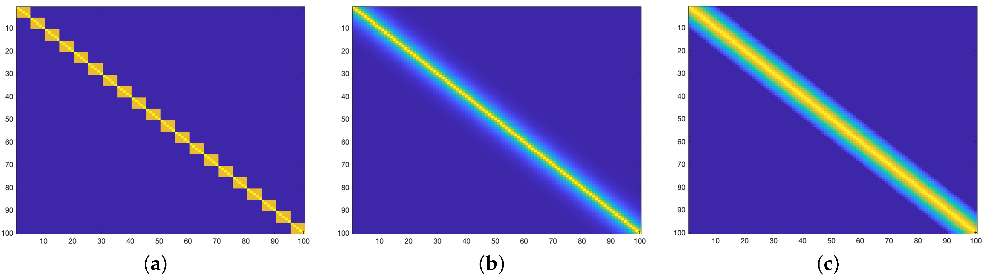
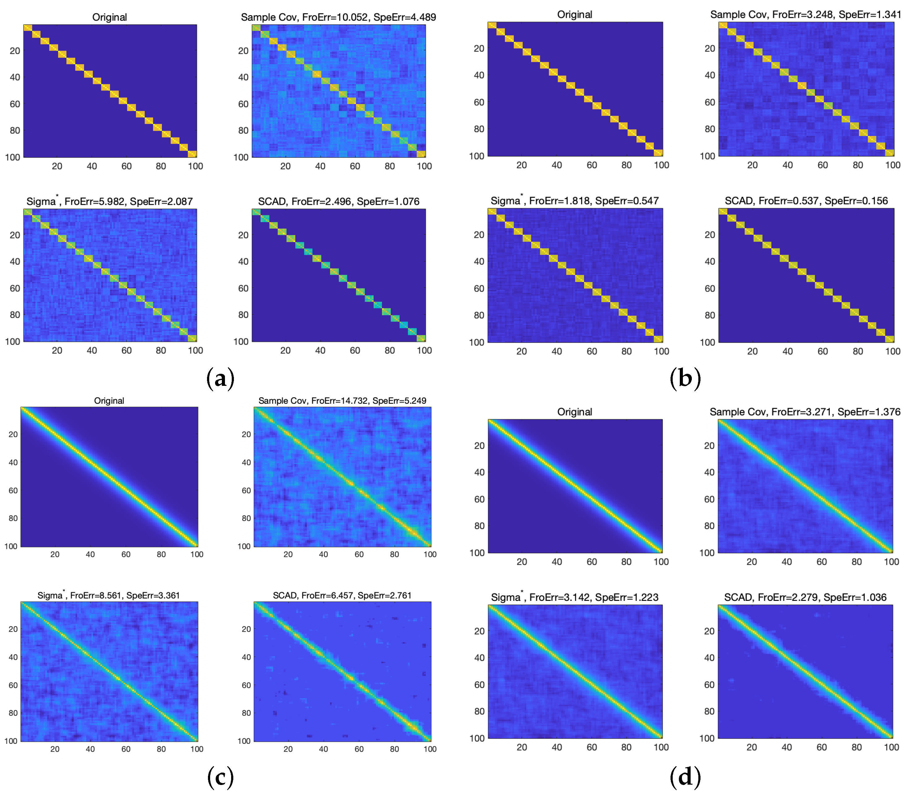
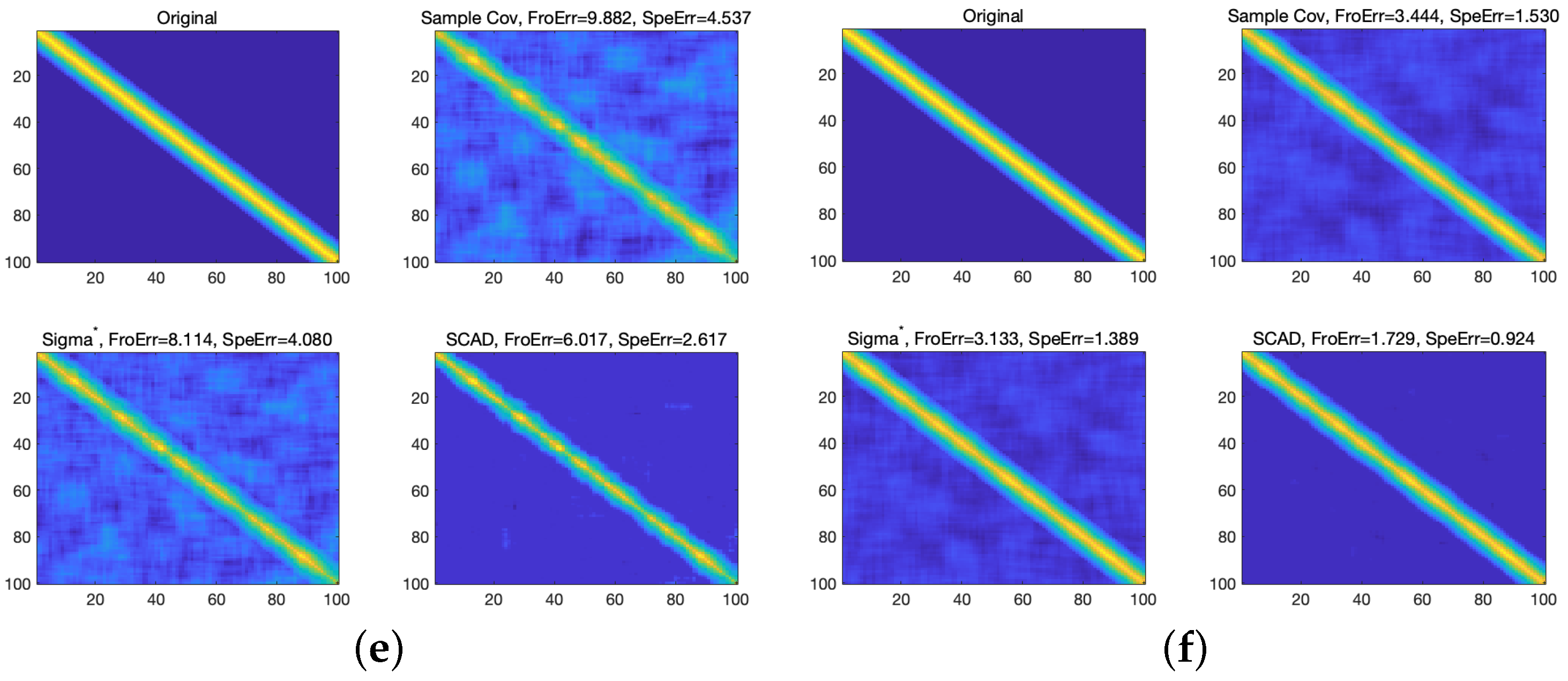
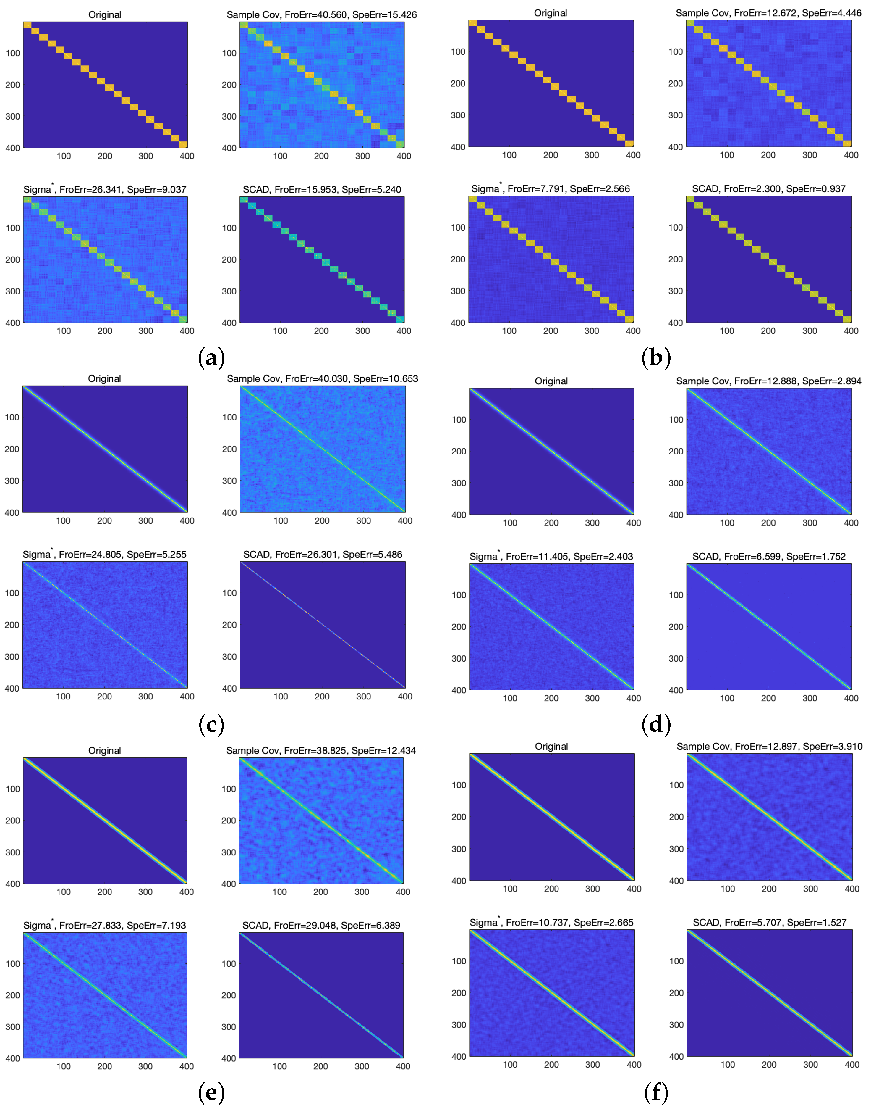
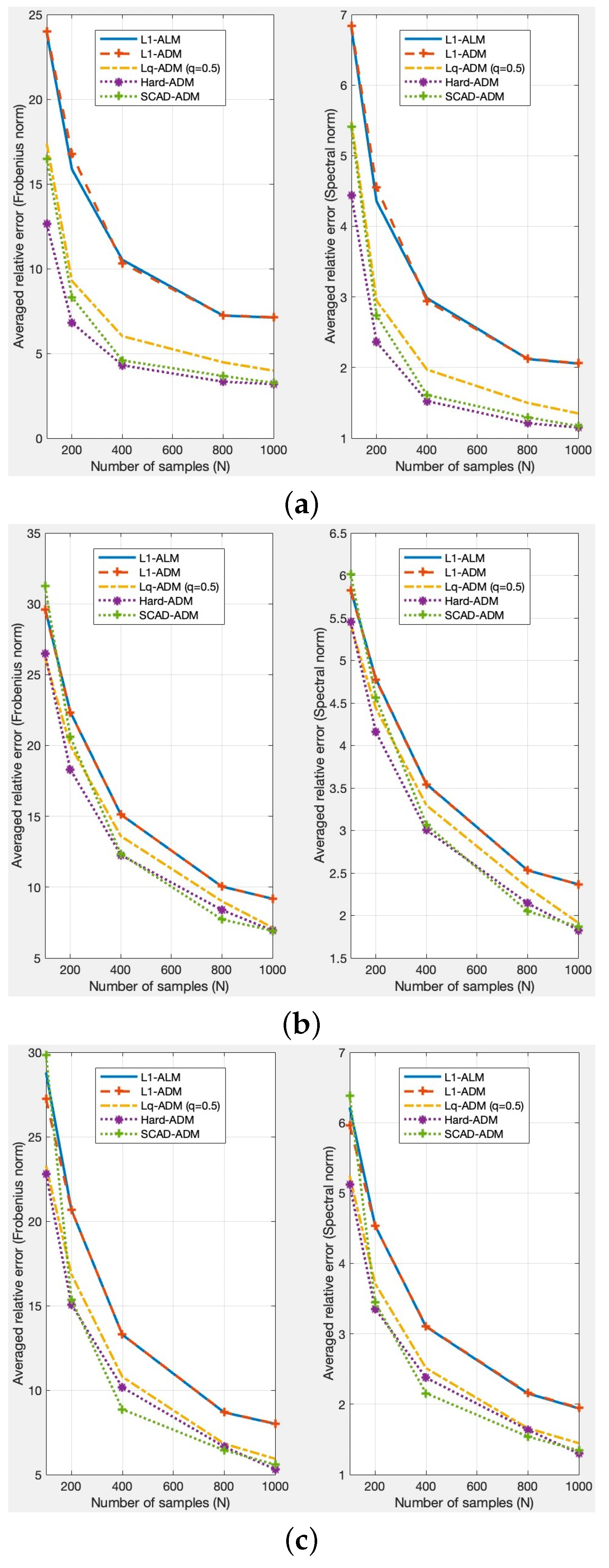
4.1.1. The Simulation of Typical Sparse Covariance Matrix

In simulation, we simulate Block matrix, Toeplitz matrix, and Banded matrix, respectively. The heat map of these three types matrix are shown in Figure 1.

We consider dimensions with d = $100,400$, the sample size $n\in \{100,200,400,800,1000\}$, and the frequency of the simulations $f=1,2,\dots ,10$. We measure the performance of the covariance matrix estimation based on the relative error of the estimation under the Frobenius norm and the spectral norm. In the process of the simulation, we first simulate the data set (the sample size is n) satisfying the Gaussian random distribution with zero mean and finite covariance. The penalty parameter $\lambda$ is set up fifteen values range from 0 to 1.

Figure 2 shows the heat maps of the estimator ${\Sigma }_{SCM}$, ${\Sigma }^{*}$ and ${\Sigma }_{SCAD}$ under the three simulation matrices when $d=100$, and the corresponding sample sizes are $n=100$ and $n=1000$, respectively. On the one hand, the error of the estimator ${\Sigma }_{SCAD}$ is always smaller than other estimators. On the other hand, the heat map of the estimator ${\Sigma }_{SCAD}$ is more and more similar to the original simulation matrix, which implies that the error of the estimator ${\Sigma }_{SCAD}$ is gradually decreasing as the sample size increases. To compare with the estimator ${\Sigma }_{L_1\left(ALM\right)}$ which using the lasso penalty function under ALM algorithm, we named the estimator using SCAD, Hard-threshold, $L_q$-norm ($q=0.5$) and lasso penalty functions under ADM as ${\Sigma }_{SCAD}$, ${\Sigma }_{Hard}$, ${\Sigma }_{L_q}$, and ${\Sigma }_{L_1}$, respectively. It shows that the estimation error of the ${\Sigma }_{SCAD}$ and ${\Sigma }_{Hard}$ are lower than other estimators under the F-norm and the spectral-norm. In sparse optimization, the choice of the penalty parameter $\lambda$ is important. In our numerical experiment, we set up five folds cross validation and select the optimal parameter $\lambda$ by minimizing the sum of cross validation errors. Also, we give the penalty parameter $\lambda$ of the estimator ${\Sigma }_{SCAD}$ under five-folds cross-validation. The results in Figure 3 shows that the total error of estimator cross-validation is relatively large when the sample size of the three matrices reaches $n=100$ for the first time, and the total error decreases and the curve tends to be stable after $f=10$. The first simulation corresponding to the number of the samples $n=100$, all three matrices obtain the minimum error sum at the penalty parameter $\lambda =0.2276$, instead of the last simulation corresponding to the samples size $n=1000$, the penalty parameters $\lambda$ of the ${\Sigma }_{SCAD}$ are $0.3727$, $0.0848$, and $0.1389$, respectively.

Figure 4 and Figure 5 show the heat maps of estimator ${\Sigma }_{SCM}$, ${\Sigma }^{*}$ and ${\Sigma }_{SCAD}$ and choice of the penalty parameter under the three simulation matrices when $d=400$. Obviously, the error of the estimator increases in Figure 4. For the penalty parameter $\lambda$, with the increase of the simulation frequencies, the error decreases significantly. The total error of the first simulation is higher than before. The first simulation corresponding to the sample size $n=100$, all three matrices obtain the minimum error sum at the penalty parameter $\lambda =0.3728$. Moreover, the last simulation corresponding to the sample size $n=1000$, and the penalty parameters $\lambda$ of the estimator ${\Sigma }_{SCAD}$ are $0.2276$, $0.0848$, and $0.0848$, respectively.

Figure 6 shows the performance of all estimators for $d=100$. We use SCAD-ADM, Hard-ADM, $L_q$-ADM, and $L_1$-ADM to terms as the estimator ${\Sigma }_{L_1\left(ALM\right)}$, ${\Sigma }_{SCAD}$, ${\Sigma }_{Hard}$, ${\Sigma }_{L_q}$, and ${\Sigma }_{L_1}$. In this case, the performance of the estimation is different under three simulated matrices. For Block matrix, the average error of estimation with Hard-threshold is the lowest under the ADM algorithm and with the SCAD penalty is the next. This implies that the larger the sample size, the better of the performance of proposed estimators with the ADM algorithm. For instance, when the sample size $n=100$, the average estimation error of the ${\Sigma }_{L_q}$, ${\Sigma }_{Hard}$ and ${\Sigma }_{SCAD}$ are approximately 64.06%, 46.24% and 60.50% of the estimator ${\Sigma }_{L_1\left(ALM\right)}$ under the Frobenius norm, while they are 74.55%, 60.70% and 73.61% under the spectral norm. When the sample size $n=1000$, the average estimation error of the estimator ${\Sigma }_{L_q\left(ADM\right)}$, ${\Sigma }_{Hard}$ and ${\Sigma }_{SCAD}$ are approximately 54.53%, 42.03% and 46.40% of the estimator ${\Sigma }_{L_1\left(ALM\right)}$ under the Frobenius norm, while they are 64.10%, 53.13% and 57.01% under the spectral norm. It should be noted that when we simulate Toeplitz matrix, the average error of each estimator has little difference under the ADM algorithm. Overall, the average error of the new estimator with the SCAD and hard-threshold penalty function is low under the ADM algorithm. For banded matrices, the new estimator with SCAD penalty function has more obvious advantages. It is easy to see that three simulated matrices are more sparse when $d=100$.

Figure 7 shows that the performance of the estimator ${\Sigma }_{SCAD}$, ${\Sigma }_{Hard}$, and ${\Sigma }_{L_q}$ are more significant when $d=400$. All estimators decline as number of the samples increases. For Block matrix, the average relative error of the proposed estimator with the ADM algorithm under the Frobenius-norm and the spectral-norm is lower than that with ALM algorithm. When the sample size $n=100$, the average estimation error of the estimator ${\Sigma }_{L_q}$, ${\Sigma }_{Hard}$ and ${\Sigma }_{SCAD}$ are approximately $72.73\%$, $52.86\%$, and $68.91\%$ of the estimator ${\Sigma }_{L_1\left(ALM\right)}$ under the Frobenius norm, while they are $80.56\%$, $65.15\%$, and $79.40\%$ under the spectral norm. Accordingly, the average error of the estimator is higher than the situation of $d=100$. Moreover, when $n=1000$, the average estimation error of the estimator ${\Sigma }_{L_q}$, ${\Sigma }_{Hard}$ and ${\Sigma }_{SCAD}$ are approximately $55.95\%$, $44.83\%$, and $45.81\%$ under the Frobenius norm, while they are $65.68\%$, $56.01\%$, and $56.91\%$ under the spectral norm. Compared to $d=100$, it shows that the performance of the estimator is more significant for Block matrix. When we simulate Toeplitz matrix, the average error of the estimator based on the ${\Sigma }_{SCAD}$ exceeds the ${\Sigma }_{L_1\left(ALM\right)}$. However, the average error of the estimator significantly declines as number of the sample increases. The average error of the ${\Sigma }_{SCAD}$ is approximately $75.44\%$ when $n=1000$. For Banded matrix, the new estimator with SCAD penalty function shows a better performance than the estimator ${\Sigma }_{L_1\left(ALM\right)}$ and ${\Sigma }_{L_1}$.

Figure 8 shows the eigenvalues of five estimators when $d=100$ and $n=200$. As can be seen, the eigenvalues of all comparison estimator are positive. This implies that the estimator is positive-definite.

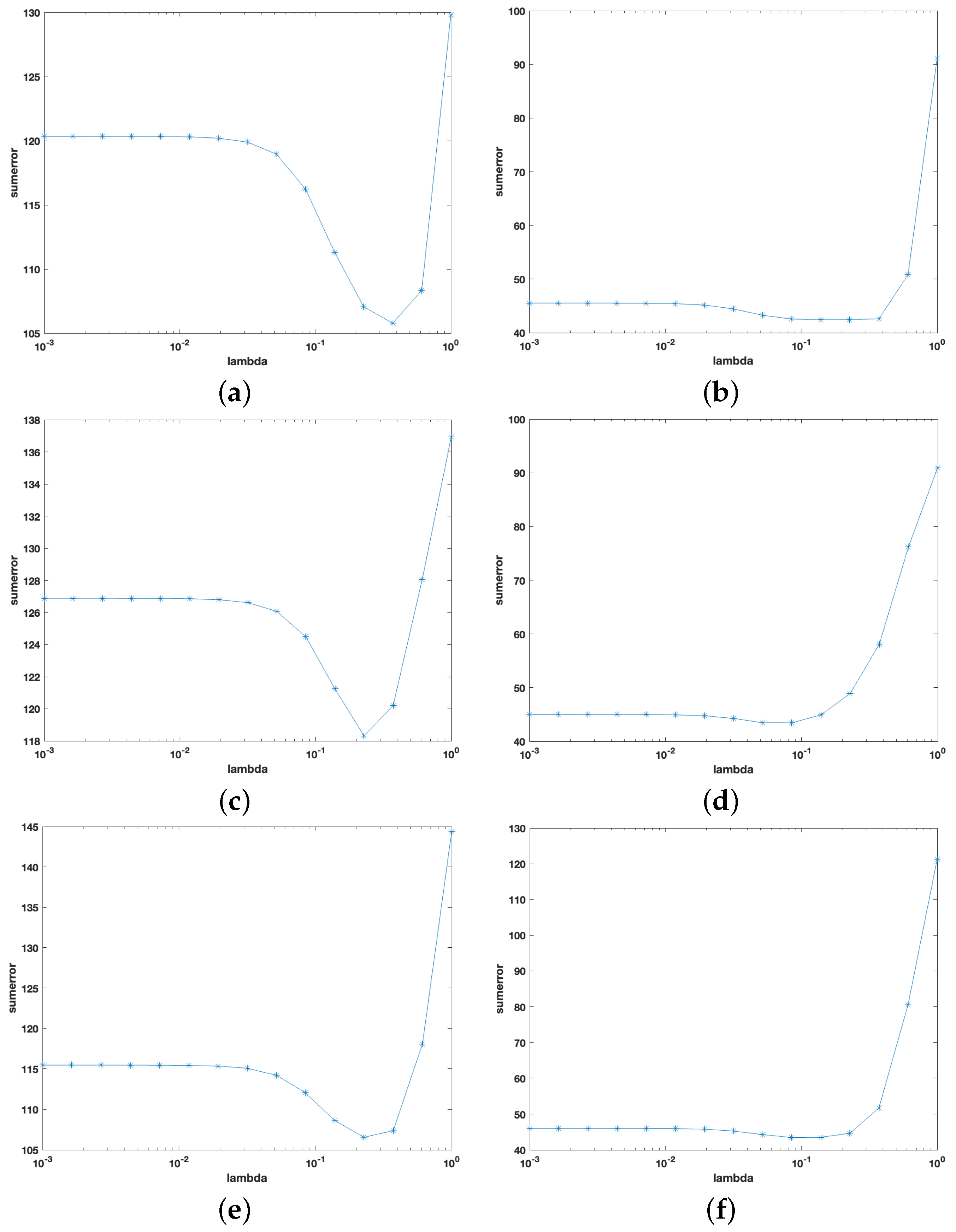
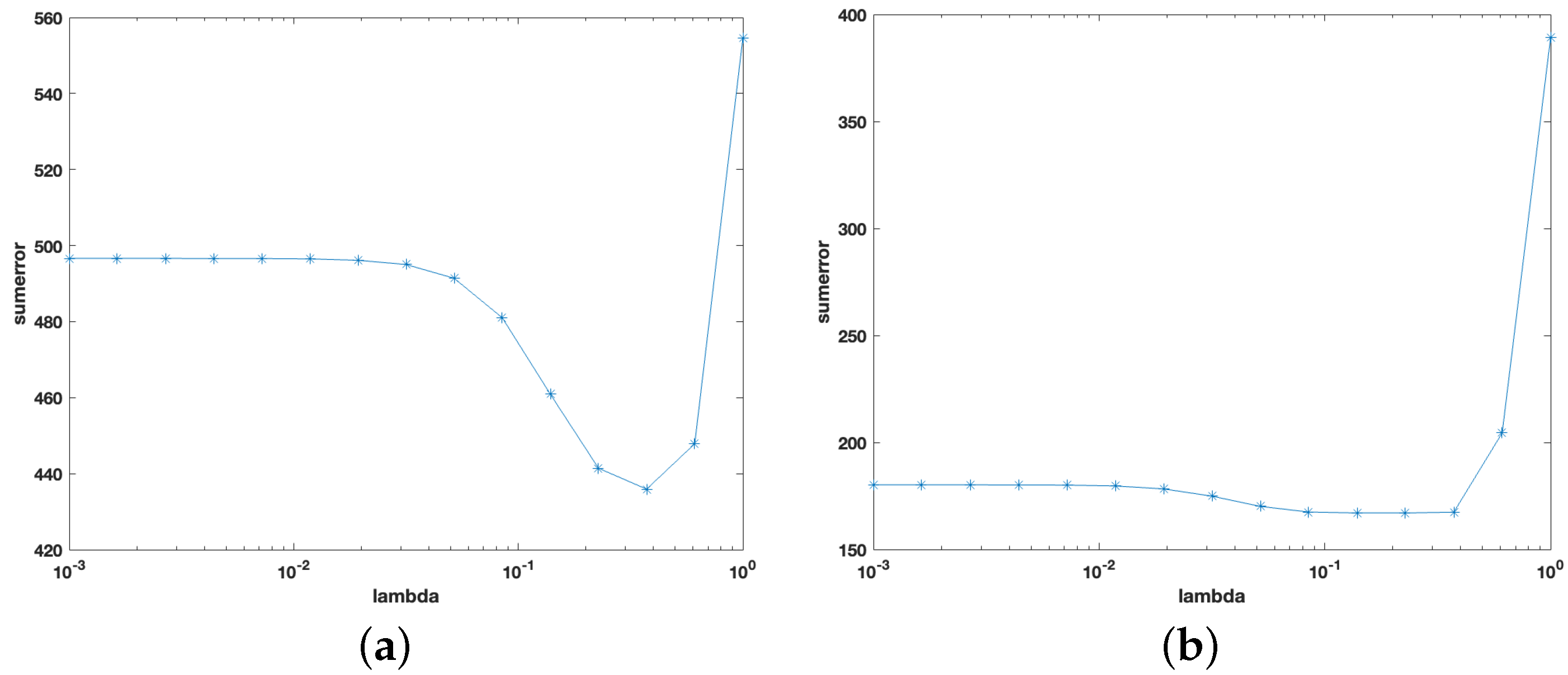
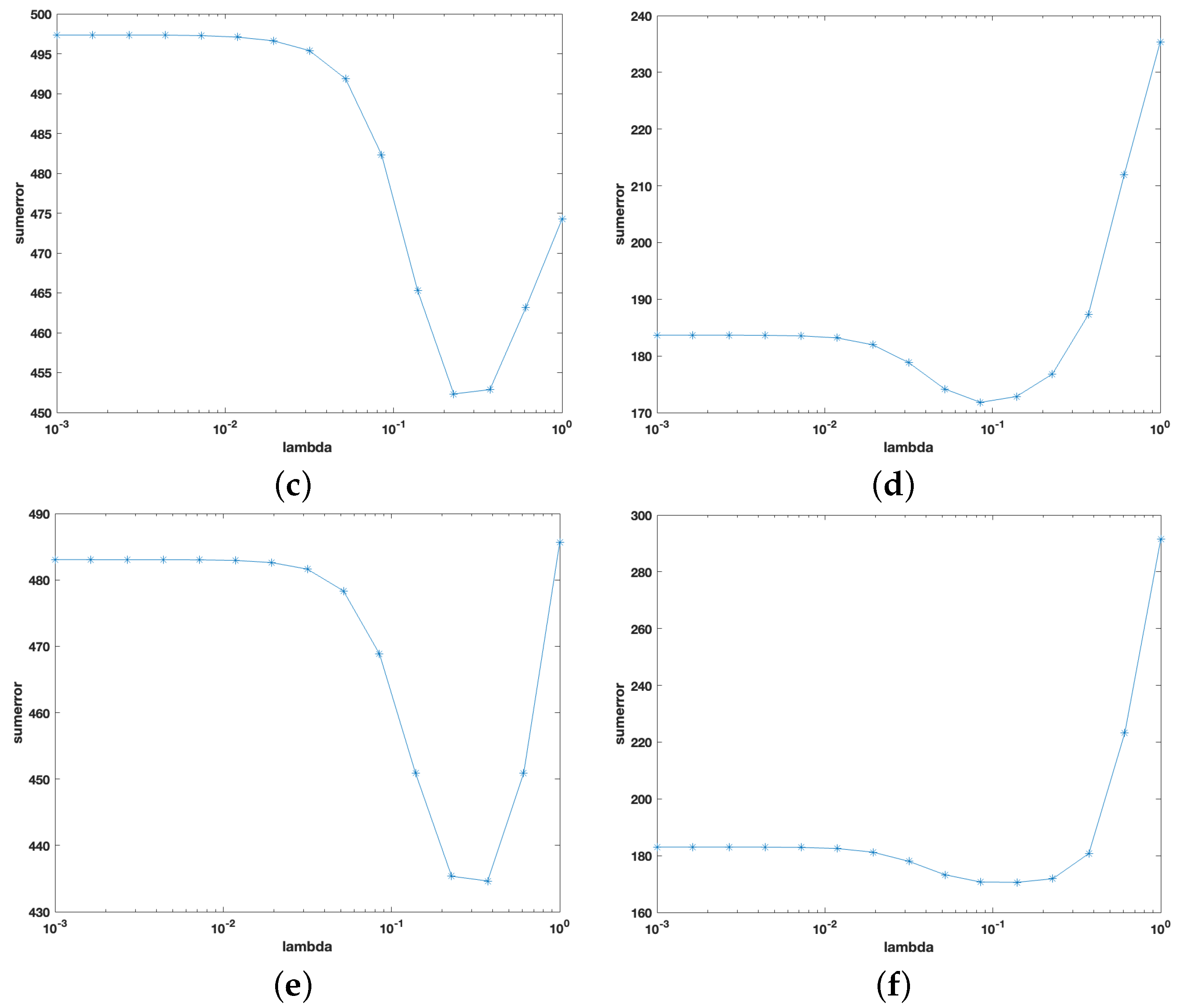
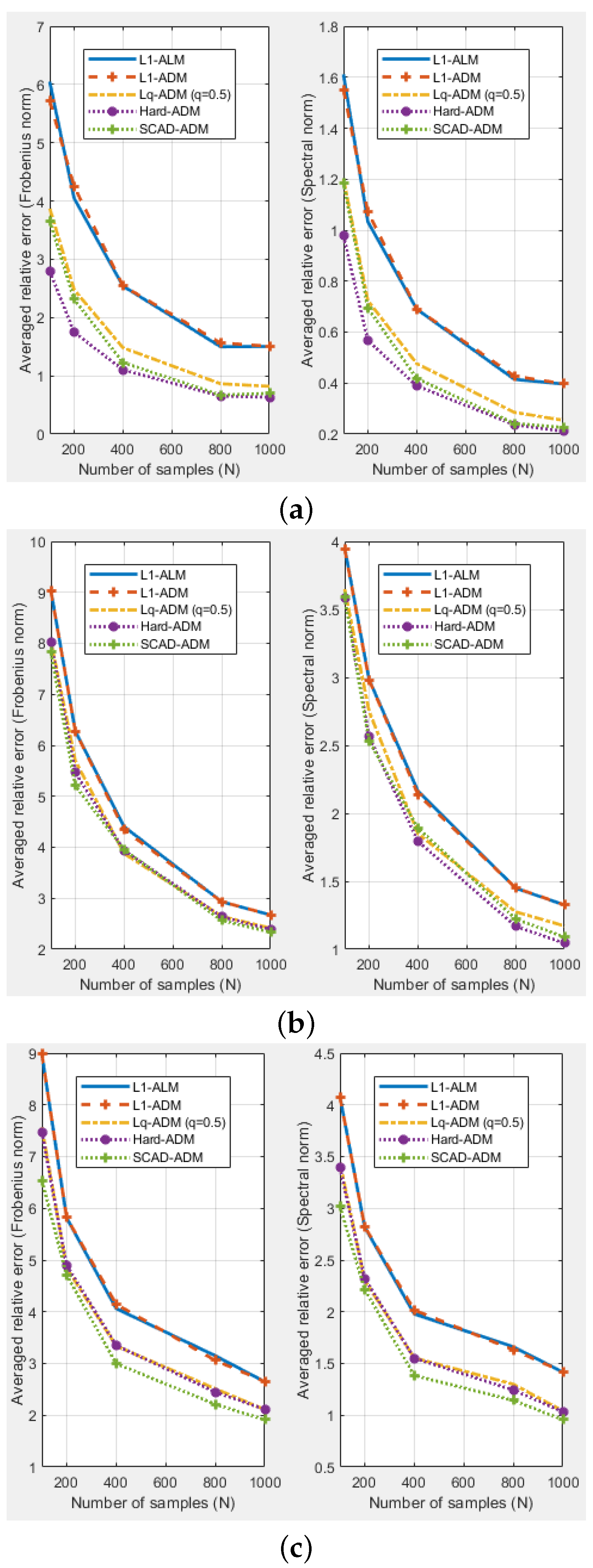
4.1.2. The Monte Carlo Simulation

In the Monte Carlo simulation, we simulate the DCC model with parameters refered to Pakel et al. [27]. In the DCC model, the univariate volatility model dynamic is governed by the GARCH model. We use the GARCH(1,1) to carry out it with parameters. We generate a simulation return, where the number of the sample $T=1000$. As for the dimension of the assets, we set three dimensions, there are $N=100,400,800$, respectively. In our simulation, the concentration ratio is $c=0.80$.

Although c can be larger than one, we only consider the situation of c is less than one so that we can compare the performance with the DCC model.

To measure the performance of the new estimator effectively, the loss function referred to Engle et al. [28] is given by

$${\mathcal{L}}_{loss}\left(\widehat{\Sigma },\Sigma \right)=\frac{N\left[tr\left({\widehat{\Sigma }}^{-1}{\Sigma }^{-1}\widehat{\Sigma }\right)\right]}{{\left[tr\left({\widehat{\Sigma }}^{-1}\right)\right]}^2}-\frac{N}{tr\left({\widehat{\Sigma }}^{-1}\right)},$$

(8)

which can be to extend to the case of the $\widehat{H_t}$, i.e.,

$$L=\frac{1}{T}\sum _{t=1}^T{\mathcal{L}}_{loss}(\widehat{H_t},H_t).$$

(9)

We first use five estimators to replace the $\overline{S}$, and then we combine them with DCC model to compare the loss (8). The following are five estimators that we consider. The explication of each estimator as follow:

• DCC-S: The $\overline{S}$ in the DCC model is replaced by the sample covariance matrix ${\Sigma }_{SCM}$.
• DCC-L2: The $\overline{S}$ in the DCC model is replaced by the estimator obtained from the method of Engle and Ledoit [7].
• DCC-NL: The $\overline{S}$ in the DCC model is replaced by the estimator obtained from the method of [18].
• DCC-NCP1: The $\overline{S}$ in the DCC model is replaced by the estimator ${\Sigma }_{Hard}$ obtained from the model (7) based on the hard-threshold penalty function.
• DCC-NCP2: The $\overline{S}$ in the DCC model is replaced by the estimator ${\Sigma }_{SCAd}$ obtained from the model (7) based on the SCAD penalty function.

The bold character in

Table 1. The loss of five estimators in different dimensions of the assets. (The unit is ${10}^{-6}$).

N	DCC-S	DCC-L2	DCC-NL	DCC-NCP1	DCC-NCP2
100	4.6874	0.6223	0.4996	0.2279	2.4265
400	3.2222	2.4103	3.1089	2.6286	0.2583
800	5.6512	4.2802	4.9354	3.7852	1.4324

denote the minimum loss under every dimension. It can be seen that the loss of the improved DCC model is smaller than that of other models. As the dimension increases, the performance of the improved DCC model is better than other DCC variants.

4.2. The Application

In order to prove the robustness of the model, we implemented the empirical research. The data of this paper come from the component stock of CSI500, HS300, and SSE50 in 218 the tushare financial website. The whole period of the samples is from 24 May 2017 to 1 July 2021. Removing the missing data of the samples from transaction, we finally obtain 426 component stocks of CSI500, 218 component stocks of HS300, and 41 component stocks of SSE50. We set $T_1=500$ as the windows of the estimation first, and then we shift these 500 days training window forward, update the portfolio at frequencies of 100 and 200 days.

4.2.1. Global Minimum Variance Portfolio

In this article, we focus on the portfolio optimization model with constraints below

$$\underset{\omega }{\min }{\omega }^{\prime }\Sigma \omega$$

$$\mathrm{s}.\mathrm{t}.\left\{\begin{array}{c}{\mathbf{1}}^{{}^{\prime }}\omega =1,\hfill \\ r^{{}^{\prime }}\omega \ge r_{min},\hfill \\ \omega \ge 0,\hfill \end{array}\right.$$

(10)

where $\mathbf{1}$ denote the vector of ones of $N\times 1$ and $\omega =({\omega }_1,{\omega }_2,\dots .,{\omega }_N)$ denote the weight vector of the assets. In what follows, we replace the $\Sigma$ in the model (10) by different effective covariance matrix estimations.

4.2.2. Analysis of Empirical Research

We apply the above five estimators to the portfolio optimization model and consider the three indexes. When the expected return achieves $0.0015$, we allow the assets to be sell short. Supposed that one year is 252 trading day, the average rate of return (MR) and standard deviation (SD) in the

Table 2. The out-of-sample performance of five estimators of 41 assets based on SSE50 in the portfolio optimization model.

Model	MR *		SD *		SR
	100 d	200 d	100 d	200 d	100 d	200 d
DCC-S	37.80	37.80	20.783	16.561	1.735	2.177
DCC-L2	37.80	37.80	20.700	16.417	1.742	2.196
DCC-NL	37.80	37.80	20.701	16.470	1.741	2.189
DDC-NCP1	37.80	37.80	20.658	16.652	1.745	2.165
DCC-NCP2	37.80	37.80	20.488	16.543	1.760	2.179

* denote the unit is %.

,

Table 3. The out-of-sample performance of five estimators of 218 assets based on HS300 in the portfolio optimization model.

Model	MR *		SD *		SR
	100 d	200 d	100 d	200 d	100 d	200 d
DCC-S	37.800	37.800	15.447	15.393	2.334	2.2.342
DCC-L2	37.800	37.800	15.305	15.174	2.355	2.376
DCC-NL	37.800	37.800	15.319	15.377	2.353	2.346
DDC-NCP1	37.800	37.800	15.271	15.418	2.367	2.338
DCC-NCP2	37.800	37.800	15.559	15.079	2.317	2.391

* denote the unit is %.

and

Table 4. The out-of-sample performance of five estimators of 426 assets based on CSI500 in the portfolio optimization model.

Model	MR *		SD *		SR
	100 d	200 d	100 d	200 d	100 d	200 d
DCC-S	37.800	37.800	13.132	13.452	2.745	2.680
DCC-L2	37.800	37.800	13.029	13.543	2.767	2.662
DCC-NL	37.800	37.800	12.906	13.384	2.793	2.693
DDC-NCP1	37.800	37.800	12.883	13.219	2.798	2.727
DCC-NCP2	37.800	37.800	12.951	13.189	2.783	2.733

* denote the unit is %.

are obtained on this premise.

Table 2, Table 3 and Table 4 show the out-of-sample performance of five portfolio optimization models with different assets. For out-of-sample data, we use the SD and Sharpe ratio as the performance metric. To obtain the Sharpe ratio with accuracy, we set the risk-free rate is 1.75% and the mean returns of all models are equal under the frequency of the 100 days and 200 days in Table 2, Table 3 and Table 4.

Table 2 shows that the SD of the DCC-NCP2 corresponding to portfolio optimization model is only $20.488\%$, which is the smallest in all models in the case of the frequency of 100 days. It achieves the highest Sharpe ratio in all models. Under the the frequency of 200 days, the performance of the portfolio optimization model corresponding to DCC-L2 is the best and the Share ratio of the portfolio optimization model corresponding to DCC-L2 is the highest in all models.

Table 3 gives the performance of the portfolio optimization models corresponding to five estimators with 218 assets. It is easy to see that the performance of the portfolio optimization model corresponding to our new model DCC-NCP1 and DCC-NCP2 are superior to other models under the frequency of 100 days and 200 days, respectively. The portfolio optimization model corresponding to our new estimator obtains the smallest SD and the highest Sharpe ratio. Therefore, the portfolio optimization model corresponding to our new estimator is superior to other models as the assets increase.

Table 4 compares the out-of-sample performance of the portfolio optimization models corresponding to each estimator with 426 assets. When the number of assets $N=426$, the information ratio is given by

$$c=\frac{N}{T}=\frac{426}{500}=0.852.$$

(11)

The result shows that the portfolio optimization model corresponding to our new estimator obtains the smallest SD in all models. Moreover, as the assets increase, the out-of-sample SD of our new estimator corresponding to portfolio optimization model has significantly reduced.

5. Discussion

In numerical simulations, we found that the error of the new estimator significantly decreases with the increase of simulation times and sample size. This is the impact of vertical size increase on the performance of the estimator. In empirical research, we use the rolling windows method to estimate and predict out-of-sample risk for the length of estimate window $T=500$. As the assets increase, the performance of the portfolio optimization model corresponding to DCC-NCP1 and DCC-NCP2 is better than other models. Obviously, the performance of the estimator has also been demonstrated when the horizontal dimension increases. As you can see, the new estimator exhibits superior performance in both aspects.

6. Conlusions

In this paper, we proposed an improved DCC model by combining the rotation invariant estimator and nonconvex penalty functions. We first developed the nonconvex optimization model of the covariance matrix estimation based on the SCAD and hard threshold penalty functions, and then we used ADM to solve the nonconvex optimization model to obtain an optimal covariance matrix estimation. Moreover, we replaced the unconditional covariance matrix $\overline{S}$ in the DCC model by the new estimations based on the SCAD and hard threshold penalty functions to get improved DCC models, respectively. Finally, we provided the numerical simulations to demonstrate that the function of loss of the proposed estimator is significantly smaller than DCC variants. In the application, we applied real stock return data to portfolio selection, we showed that the portfolio optimization model corresponding to new estimator obtains the higher Sharpe ratio as the number of assets increases.

In addition, since the traditional DCC model and some DCC model variants generally need to implement a normalization step of the correlation dynamics or use some window-based local correlation matrices as proxies of the instantaneous correlation matrix, these processes may affect the model fitting or complicate the theoretical analysis [20,21]. Thus, an interesting future research problem is to use the nonconvex optimization model to estimate the angular correlation matrix in dynamical conditional angular correlation model and apply it to portfolio construction in high-dimensional financial data.

References

1. Engel, J.; Buydens, L.; Blanchet, L. An overview of large-dimensional covariance and precision matrix estimators with applications in chemometrics. J. Chemom. 2017, 31, e2880. [Google Scholar] [CrossRef]
2. Fan, J.; Liao, Y.; Liu, H. An overview of the estimation of large covariance and precision matrices. Econom. J. 2016, 19, C1–C32. [Google Scholar] [CrossRef]
3. Tong, T.; Wang, C.; Wang, Y. Estimation of variances and covariances for high-dimensional data: A selective review. Wiley Interdiscip. Rev. Comput. Stat. 2014, 6, 255–264. [Google Scholar] [CrossRef]
4. Stein, C. Lectures on the theory of estimation of many parameters. J. Sov. Math. 1986, 34, 1373–1403. [Google Scholar] [CrossRef]
5. Engle, R.F.; Ledoit, O.; Wolf, M. Large dynamic covariance matrices. J. Bus. Econom. Stat. 2019, 37, 363–375. [Google Scholar] [CrossRef]
6. Ledoit, O.; Wolf, M. Nonlinear shrinkage of the covariance matrix for portfolio selection: Markowitz meets goldilocks. Rev. Financ. Stud. 2018, 30, 4349–4388. [Google Scholar] [CrossRef]
7. Ledoit, O.; Wolf, M. Honey, I shrunk the sample covariance matrix. J. Portfolio. Mange. 2004, 30, 110–119. [Google Scholar] [CrossRef]
8. Bickel, P.J.; Elizaveta, L. Covariance regularization by thresholding. Ann. Stat. 2008, 36, 2577–2604. [Google Scholar] [CrossRef]
9. Rothman, A.J.; Bickel, P.J.; Levina, E.; Zhu, J. Sparse permutation invariant covariance estimation. Electron. J. Stat. 2008, 2, 494–515. [Google Scholar]
10. Balmand, S.; Dalalyan, A.S. On estimation of the diagonal elements of a sparse precision matrix. Electron. J. Stat. 2016, 10, 1551–1579. [Google Scholar]
11. Ravikumar, P.; Wainwright, M.J.; Raskutti, G.; Yu, B. High-dimensional covariance estimation by minimizing L1-penalized log-determinant divergence. Electron. J. Stat. 2011, 5, 935–980. [Google Scholar] [CrossRef]
12. Zhou, S.; Xiu, N.H.; Luo, Z.; Kong, L.C. Sparse and low-rank covariance matrix estimation. J. Oper. Res. Soc. China 2015, 3, 231–250. [Google Scholar] [CrossRef]
13. Fan, J.; Li, R. Variable selection via nonconcave penalized likelihood and its oracle properties. J. Am. Stat. Assoc. 2001, 96, 1348–1360. [Google Scholar] [CrossRef]
14. Fan, J.; Peng, J. Nonconcave penalized likelihood with a diverging number of parameters. Ann. Stat. 2004, 32, 928–961. [Google Scholar] [CrossRef]
15. Engle, R. Dynamic conditional correlation: A simple class of multivariate generalized autoregressive conditional heteroskedasticity models. J. Bus. Econom. Stat. 2002, 20, 339–350. [Google Scholar] [CrossRef]
16. Bollerslev, T. Generalized autoregressive conditional heteroskedasticity. EERI Res. Paper. 1986, 31, 307–327. [Google Scholar] [CrossRef]
17. Bollerslev, T. Modeling the coherence in short-run nominal exchange rates: A multivariate generalized ARCH model. Rev. Econ. Stat. 1990, 72, 498–505. [Google Scholar] [CrossRef]
18. Ledoit, O.; Wolf, M. Nonlinear shrinkage estimation of large-dimensional covariance matrices. Ann. Stat. 2012, 40, 1024–1060. [Google Scholar] [CrossRef]
19. De Nard, G.; Engle, R.F.; Ledoit, O.; Wolf, M. Large dynamic covariance matrices: Enhancements based on intraday data. J. Bank. Financ. 2022, 138, 1–16. [Google Scholar] [CrossRef]
20. Jarjour, R.; Chan, K.S. Dynamic conditional angular correlation. J. Econom. 2020, 216, 137–150. [Google Scholar] [CrossRef]
21. Tse, Y.K.; Tsui, A.K.C. A multivariate generalized autoregressive conditional heteroscedasticity model with time-varying correlations. J. Bus. Econom. Stat. 2002, 20, 51–362. [Google Scholar] [CrossRef]
22. Yuan, X.; Yu, W.; Yin, Z.X.; Wang, G.Q. Improved large dynamic covariance matrix estimation with graphical lasso and its application in portfolio selection. IEEE Access 2020, 8, 189179–189188. [Google Scholar] [CrossRef]
23. Wen, F.; Yang, Y.; Liu, L.P.; Qiu, R.C. Positive definite estimation of large covariance matrix using generalized non-convex penalties. IEEE Access 2016, 4, 4168–4182. [Google Scholar] [CrossRef]
24. Zhang, Y.; Tao, J.Y.; Yin, Z.X.; Wang, G.Q. Improved large covariance matrix estimation based on efficient convex combination and its application in portfolio optimization. Mathematics 2022, 10, 4282. [Google Scholar] [CrossRef]
25. Ledoit, O.; Wolf, M. Quadratic shrinkage for large covariance matrices. Bernoulli 2022, 28, 1519–1547. [Google Scholar] [CrossRef]
26. Antoniadis, A. Wavelets in Statistics: A Review (with discussion). J. Ital. Stat. Soc. 1997, 6, 97–130. [Google Scholar] [CrossRef]
27. Pakel, C.; Shephard, N.; Sheppard, K.; Engle, R.F. Fitting vast dimensional time-Varying covariance models. J. Bus. Econ. Stat. 2021, 39, 652–668. [Google Scholar] [CrossRef]
28. Hafner, C.M.; Reznikova, O. On the estimation of dynamic conditional correlation models. Comput. Stat. Data Anal. 2012, 56, 3533–3545. [Google Scholar] [CrossRef]
Figure 1. The simulated matrices for d = 100 . (a) Simulation matrix-Block matrix; (b) Simulation matrix-Toeplitz matrix; (c) Simulation matrix-Banded matrix.
Symmetry 15 00953 g001
Figure 2. The heat map of each estimation for d = 100 . (a) Block matrix ( d = 100 , n = 100 ); (b) Block matrix ( d = 100 , n = 1000 ); (c) Block matrix ( d = 100 , n = 100 ); (d) Block matrix ( d = 100 , n = 1000 ); (e) Block matrix ( d = 100 , n = 100 ); (f) Block matrix ( d = 100 , n = 1000 ).
Symmetry 15 00953 g002aSymmetry 15 00953 g002b
Figure 3. The sum error of the estimator Σ S C A D in five folds cross-validation under the F-norm for d = 100 . (a) Block matrix ( f = 1 , n = 100 ); (b) Block matrix ( f = 10 , n = 1000 ); (c) Block matrix ( f = 1 , n = 100 ); (d) Block matrix ( f = 1 , n = 100 ); (e) Block matrix ( f = 10 , n = 1000 ); (f) Block matrix ( f = 1 , n = 100 ).
Symmetry 15 00953 g003
Figure 4. The heat map of each estimator for d = 400 . (a) Block matrix ( d = 400 , n = 100 ); (b) Block matrix ( d = 400 , n = 1000 ); (c) Block matrix ( d = 400 , n = 100 ); (d) Block matrix ( d = 400 , n = 1000 ); (e) Block matrix ( d = 400 , n = 100 ); (f) Block matrix ( d = 400 , n = 1000 ).
Symmetry 15 00953 g004
Figure 5. The sum error of the estimator Σ S C A D in five folds cross-validation under the F-norm for d = 400 . (a) Block matrix ( f = 1 , n = 100 ); (b) Block matrix ( f = 10 , n = 1000 ); (c) Block matrix ( f = 1 , n = 100 ); (d) Block matrix ( f = 1 , n = 100 ); (e) Block matrix ( f = 10 , n = 1000 ); (f) Block matrix ( f = 1 , n = 100 ).
Symmetry 15 00953 g005aSymmetry 15 00953 g005b
Figure 6. The average relative error of each estimator for d = 100 . (a) Simulation matrix-Block matrix; (b) Simulation matrix-Toeplitz matrix; (c) Simulation matrix-Banded matrix.
Symmetry 15 00953 g006
Figure 7. The average relative error of each estimator for d = 400 . (a) Simulation matrix-Block matrix; (b) Simulation matrix-Toeplitz matrix; (c) Simulation matrix-Banded matrix.
Symmetry 15 00953 g007
Figure 8. The eigenvalues of each estimation under Block matrix for d = 100 and n = 200 .
Symmetry 15 00953 g008