Article

Chikungunya Transmission of Mathematical Model Using the Fractional Derivative

by
Sonal Jain
1 and
Dimplekumar N. Chalishajar
2,*
1
School of Technology, Woxsen University, Hyderabad, Telangana, Pin 502345, India
2
Department of Applied Mathematics, Mallory Hall, Virginia Military Institute (VMI), Lexington, VA 24450, USA
*
Author to whom correspondence should be addressed.
Symmetry 2023, 15(4), 952; https://doi.org/10.3390/sym15040952
Submission received: 1 March 2023 / Revised: 16 March 2023 / Accepted: 18 April 2023 / Published: 21 April 2023
(This article belongs to the Section Mathematics)

Abstract

:
In this study, a mathematical model that may depict the dynamic transmission of the Chikungunya virus within a specific population has been examined. Various differential operators were considered, ranging from classical to nonlocal operators. We added a stochastic component to each instance and used the Lipschitz and linear growth criteria to illustrate the existence and uniqueness of the solutions. The most recent numerical method with Newton polynomial (are related symmetrical) interpolations was used to solve each problem numerically using MATLAB. There are some presented numerical simulations which are compared with the Lipschitz and linear growth properties. This new research work emphasizes how the Chikungunya virus model is formulated using fractional ODEs.

1. Introduction

A challenging and crucial area of modern mathematical control theory and harmonic analysis, which has many applications and is of interest to many academics worldwide, is the investigation of systems with symmetry and control systems. Due to recently developed, highly potent mathematical techniques, such as decay, the power law, and crossover from power law to exponential, which can capture even the most subtle complexities of nature, the idea of fractional calculus operators have been consolidated to create new fractional integration and differentiation operators in many issues in the real world. These novel operators’ key benefit is their ability to simultaneously capture processes that follow power laws, Mittag-Leffler functions, and exponential decay functions [1,2,3,4]. In [5], the authors developed an application software for computing the components of the stress-strain state of biomaterials while taking into account their fractal structure using the finite element method to calculate the rheological properties of a biomaterial with a fractal structure. These new operators are ideal modeling tools for many complicated real-world issues thanks to their exceptional and distinctive capabilities. Mathematicians also developed the idea of Brownian motion to capture randomness. Over the past ten years, this idea has been employed with varying degrees of success in a number of sectors of science, technology, and engineering. It is important to keep in mind that Brownian motions and differential operators with the aforementioned kernels cannot take into account randomness, fading memory, crossover effects, and power law, even though both have proved successful in replicating real-world problems separately [6,7,8]. However, it is important to remember that many situations in nature can display both processes. Therefore, neither stochastic nor fractional calculus are unable to account for these. Since the spread of infectious diseases within humans depends on a variety of conditions, it is true that their dissemination cannot be well explained by straightforward mathematical formulae. The Chikungunya virus, for instance, spread. This spread has been the subject of numerous mathematical models; therefore, it is thought that these new operators will play a major role in modeling in the future. The spread is modeled in this paper using fractional operators.
Several methods, including residual power series, symmetry, spectral, Fourier transform, similarity, and collocation methods, are being used to examine the system with symmetry and manage differential equations in both fractional and classical orders, as well as their systems. A symmetry fractional operator and the various types of Caputo derivatives are directly related. Due to the elegant form of its fractional definition and its algebraic features, the concept of the fractional derivative operator plays a significant role in the fields of mathematical inequality and mathematical analysis. Numerous authors have recently investigated the tight connections and related work on fractional operators with symmetry. Because of their close association, when working on one topic, it can also be used to the other.
Today, mathematical modeling is regarded as an essential and successful method for describing the origin and dynamics of many prevalent infectious diseases, including HIV/AIDS, COVID-19, TB, Lassa fever, Ebola, syphilis, cancer cells, polio, and many others, which are categorized in [9]. Due to its nonlocal features and memory effects, a fractional-order derivative, which is thought of as an extension of the integer-order derivative, has attracted much scholarly attention recently. The fractional-order derivatives have memory features since they depend on all of the prior states in addition to the current state [10]. Several academics have used the idea of fractional calculus to simulate various nonlinear phenomena in the fields of medicine, engineering, physics, and applied sciences. This is due to the specific qualities of fractional calculus. For instance, Diethelm [11] confirmed in his work that the proposed fractional-order model more closely matches the actual data of the dengue sickness than the integer-order case. Bi-order derivatives have been taken into consideration in an unique differentiation theory that has been put forth recently; the first case is known as the fractal fractional-order and the second case is known as the fractal dimension. In the literature, this kind of integral and differential equation is still not well covered. Recently, Pitolli [12] has effectively studied the Riesz-Caputo derivative in a cubic spline to approximate the numerical solution of the boundary value differential problems and compare the same with analytical solutions. Several numerical schemes have been implemented to study nonlinear fractional systems. The discretization methods for the logistic equation are discussed by Izadi and Shrivastava [13].
In the current study, the fractional case extension of the classical-order differential equations is discussed. The idea of a fractional operator has been successfully used to describe a variety of real-world issues in engineering, physics, biology, and biomedical systems. In order to describe the Chikungunya differential equations in the sense of the Caputo operator, this work extends the notion of fractional operators of orders. We are not aware of any formulations of the Chikungunya model that incorporate fractional derivatives.
The primary body of this work is divided into the following sections:
Section 2 provides some helpful definitions of fractional operators. Section 3 introduces the dynamics of the Chikungunya model for cases of integer and non-integer order, and Section 4 examines linear stability analysis, the existence, and the uniqueness of solutions via the fractional operators presented in Section 4. In Section 5, a novel numerical approximation method for the proposed model’s solution, which is described by the Caputo-fractional, Caputo-Fabrizio (CF), and AB derivatives, and numerical experiments that illustrate the behavior of the dynamics under investigation are presented for various instances of orders, followed by a numerical simulation of various orders. The validation of current study is elaborated in the form of a remark. Finally, the conclusion is presented with details of the limitations and future work.

2. Preliminaries and Definition

In this section, we review some fundamental definitions and characteristics of the theory of fractional calculus that will be helpful in the sections to follow.
Definition 1
([14]). The Caputo derivative with ζ order, where u is a function not necessarily differentiable and ζ is a real number such that ζ > 0 is given as:
0 C D t ζ u ( t ) = 1 Γ ( ζ ) 0 t ( t y ) ζ 1 u ( y ) d y .
Definition 2
([15]). The Caputo-Fabrizio derivative for u H 1 ( a , b ) ,   b > a ,   ζ [ 0 , 1 ] of the fractional order is given by:
D t ζ ( u ( t ) ) = M ( ζ ) ( 1 ζ ) a t u ( x ) exp ζ t x 1 ζ d x .
where  M ( 0 ) = M ( 1 ) = 1  [15].
Definition 3
([16]). The AB derivative in a Caputo sense for u H 1 ( x , y ) ,   y > x ,   ζ [ 0 , 1 ] with the function u differentiable is given as:
a A B C D t ζ [ u ( t ) ] = M ( ζ ) 1 ζ a t d d t u ( x ) E ζ ζ ( t x ) ζ 1 ζ d x .
Definition 4
([16]). The Atangana-Baleanu fractional integral is given as:
a A B C I t ζ [ u ( t ) ] = 1 ζ B ( ζ ) u ( t ) + ζ B ( ζ ) Γ ( ζ ) a t u ( j ) ( t j ) ζ 1 d j .

3. Chikungunya Transmission Mathematical Model

Here, we look at a mathematical model that shows how the Chikungunya virus dynamically spreads over a particular population [17]. When bitten by an infectious mosquito, a fraction of susceptible humans S are exposed to the infection E. People then become symptomatically infectious (I) or asymptotically infectious ( I a ) after the latent phase of infection before recovering (R). Similar to this, after receiving an infectious bite, a certain percentage of susceptible mosquitoes ( X ) are exposed to the pathogen ( Y ) before developing the infectious (Z) disease. The associated equations that represent the kinetics of infection are as follows:
d S d t = β 1 S Z , d E d t = β 1 S Z λ 1 E , d I d t = ϕ λ 1 E γ I , d I a d t = ( 1 ϕ ) λ 1 E γ I a , d R d t = γ ( I + I a ) , d X d t = μ β 2 X ( I + I a ) μ X , d Y d t = β 2 X ( I + I a ) λ 2 Y μ Y , d Z d t = λ 2 Y μ z .
The following lists the Chikungunya model’s parameters and variables:
  • S represents susceptible hosts;
  • E represents exposed hosts;
  • I represents symptomatically infectious hosts;
  • I a represents asymptomatically infectious hosts (proportion);.
  • R represents recovered hosts;
  • X represents susceptible mosquitoes;
  • Y represents exposed mosquitoes;
  • Z represents infectious mosquitoes;
  • β 1 represents mosquito-to-human transmission (number of mosquito bites per human per day, allowing for imperfect pathogen transmission);
  • β 2 represents human-to-mosquito transmission (per day bite rate also allowing for imperfect pathogen transmission);
  • ϕ shows hosts that develop symptoms;
  • 1 λ 1 represents host latent period (from ‘infected’ to ‘infectious’, days);
  • 1 λ 2 represents mosquito latent period (from ‘infected’ to ‘infectious’, days);
  • γ represents host recovery rate (per day);
  • 1 ω 1 represents host pre-patient period (from ‘infected’ to symptom’s development, days);
  • μ is given by mosquito life span (days).

4. Existence and Uniqueness

We outline the model’s existence and uniqueness requirements.
For this, we demonstrate that ι 1 , 2 , 3 , 4 , 5 , 6 , 7 , 8
(a)
The linear growth condition is p ι ( X ι , ø ) 2 and G ι ( X ι , ø ) 2 k ( 1 + | X ι | 2 ) .
(b)
p ι ( X ι 1 , ø ) p ι ( X ι 2 , ø ) 2 k ¯ | X ι 1 X ι 2 | 2 G ι ( X ι 1 , ø ) G ι ( X ι 2 , ø ) 2 k ¯ | X ι 1 X ι 2 | 2 p 1 ( S , t ) = β 1 S Z , G 1 ( S , t ) = σ 1 S
p 1 ( S , t ) 2 = β S Z 2 = β 2 | S | 2 | Z | 2 β 2 ( 1 + | S | 2 ) | Z | 2 β 2 ( 1 + | S | 2 ) sup t [ 0 , t ] | Z | 2 β 2 Z 2 ( 1 + | S | 2 ) k 1 ( 1 + | S | 2 ) n u m d e n
So
G 1 ( S , t ) 2 E 1 2 ( 1 + | S | 2 ) k 1 ( 1 + | S | 2 )
p 2 ( E , t ) = β S Z λ 1 E 1 , G 2 ( E , t ) = σ 2 E
p 2 ( E , t ) 2 2 β 2 S 2 Z 2 2 λ 1 2 | E | 2 2 β 2 S 2 Z 2 1 + λ 1 2 | E | 2 2 β 2 S 2 Z 2 .
If λ 1 2 | E | 2 2 β 2 S 2 Z 2 < 1 , then
p 2 ( E , t ) 2 k 2 ( 1 + | E | 2 )
where k 2 = 2 β 2 S 2 Z 2 . Clearly also
G 2 ( E , t ) 2 σ 2 2 ( 1 + | E | 2 ) k 2 2 ( 1 + | E | 2 ) .
Furthermore,
G ι ( X ι , t ) 2 σ ι 2 ( 1 + | X ι | 2 ) k ι 2 ( 1 + | X ι | 2 )
p 3 ( I , t ) 2 = ϕ λ 1 E r I 2 2 ϕ 2 λ 2 E 2 + 2 r 2 | I | 2 2 ϕ 2 λ 2 E 2 1 + r 2 | I | 2 2 ϕ 2 λ 2 E 2 .
If
r 2 ϕ 2 λ 1 2 E 2 < 1
then
p 3 ( I , t ) 2 k 3 ( 1 + | I | 2 )
p 4 ( I , t ) 2 2 ( 1 ϕ ) 2 λ 1 2 E 2 + 2 r 2 | I a | 2 .
Thus, if
r 2 2 ( 1 ϕ ) 2 λ 1 2 E 2 < 1
then
p 4 ( I , t ) 2 k 4 ( 1 + | I a | 2 )
k 4 = 2 ( 1 ϕ ) 2 λ 1 2 E 2
p 5 ( R , t ) 2 2 r 2 I 2 + I a 2 ( 1 + R 2 ) k 5 ( 1 + R 2 )
p 6 ( X , t ) 2 3 μ 2 + 3 β 2 2 I 2 + I a 2 μ 2 | X | 2 3 μ 2 1 + β 2 2 ( I 2 + I a 2 ) μ 2 | X | 2 3 μ 2 .
If
β 2 2 ( I 2 + I a 2 ) μ 2 3 μ 2 < 1
then
p 6 ( X , t ) 2 3 μ 2 ( 1 + | X | 2 )
p 7 ( Y , t ) 2 2 β 2 2 X 2 2 ( I 2 + I a 2 ) + 2 ( λ 2 + μ ) 2 2 β 2 2 X 2 2 I 2 + I a 2 1 + ( λ 2 + μ ) 2 4 β 2 2 X 2 I 2 + I a 2 .
Thus, if
λ 2 + μ 4 β 2 2 X 2 I 2 + I a 2 < 1
then
p 7 ( Y , t ) 2 k 7 ( 1 + | X | 2 ) .
Finally, we have
p 8 ( Z , t ) 2 λ 2 2 Y 2 + μ 2 | Z | 2 λ 2 2 Y 2 1 + μ 2 | Z | 2 λ 2 2 Y 2 .
If
μ 2 λ 2 2 Y 2 < 1
then
p 9 ( Z , t ) 2 k 8 ( 1 + | Z | 2 ) .
The solution for the system is unique if
min λ 1 2 2 β 2 S 2 Z 2 , r 2 2 ( 1 ϕ ) 2 λ 1 2 E 2 , r 2 ϕ 2 λ 1 2 E 2 , β 2 2 ( I 2 + I a 2 ) 3 , λ 2 + μ 4 β 2 2 X 2 I 2 + I a 2 < 1 .
This proof holds true for both the model with a fractional derivative and the model without a fractional derivative.
Remark 1.
SIR-type models describe infection prevalence (not incidence). In order to compare weekly incidence data with our model output, new infections were tracked each day using the SEIR model studied here. The ranges for the biological components of the dynamical model are provided in the literature but the same can be calculated/implemented more accurately using fractional orders of the components, e.g., the basic reproduction number (and type reproduction number) of Chikungunya is more accurate using the fractional order system. In this context, our work is the generalization of the work by Yakoob et al. [17].

5. Numerical Methods of the Model

In this section, we provide a numerical framework for the fractional model based on the fractional derivatives of Caputo, CF, and Atangana-Baleanu [18]. We first take into account the following non-linear fractional ODEs while implementing this scheme.

5.1. Numerical Method for Caputo Fractional Derivative

We focus on the following Cauchy problem
0 C D t m ( t ) = m ( t , m ( t ) ) , m ( 0 ) = m 0
where the Caputo fractional derivative is the derivative. Now, our goal is to outline a numerical plan for resolving the previous equation. First, we convert the aforementioned equation into
m ( t ) m ( 0 ) = 1 Γ ( ) 0 t m ( ø , m ( ø ) ) ( t ø ) 1 d ø .
Here, t ξ + 1 = ( ξ + 1 ) Δ t ,
m ( t ξ + 1 ) m ( 0 ) = 1 Γ ( ) 0 t ξ + 1 m ( ø , m ( ø ) ) ( t ξ + 1 ø ) 1 d ø .
Furthermore, we have
m ( t ξ + 1 ) = m ( 0 ) + 1 Γ ( ) ϵ = 2 ξ t ϵ t ϵ + 1 m ( ø , m ( ø ) ) ( t ξ + 1 ø ) 1 d ø .
When the Newton polynomial is substituted into the equation above, we have
m ξ + 1 m 0 = 1 Γ ( ) ϵ = 2 ξ t ϵ t ϵ + 1 + m ( t ϵ 1 , m ϵ 1 ) + m ( t ϵ 1 , m ϵ 1 ) m ( t ϵ 2 , m ϵ 1 ) Δ t ( ø t ϵ 2 ) + m ( t ϵ , m ϵ 2 ) 2 m ( t ϵ 1 , m ϵ 1 ) + m ( t ϵ 2 , m ϵ 1 ) 2 ( Δ t ) 2 × ( ø t ϵ 2 ) ( ø t ϵ 1 ) ( t ξ + 1 ø ) 1 d ø .
So the above equation becomes
m ξ + 1 = m 0 + 1 Γ ( ) ϵ = 2 ξ + t ϵ t ϵ + 1 m ( t ϵ 2 , m ϵ 1 ) ( t ξ + 1 ø ) 1 d ø + t ϵ t ϵ + 1 m ( t ϵ 1 , m ϵ 1 ) m ( t ϵ 2 , m ϵ 1 ) Δ t t ϵ t ϵ + 1 ( ø t ϵ 2 ) ( t ξ + 1 ø ) 1 d ø + t ϵ t ϵ + 1 m ( t ϵ , m ϵ 2 ) 2 m ( t ϵ 1 , m ϵ 1 ) + m ( t ϵ 2 , m ϵ 1 ) 2 ( Δ t ) 2 × ( ø t ϵ 2 ) ( ø t ϵ 1 ) ( t ξ + 1 ø ) 1 d ø .
After rearranging the equation
m ξ + 1 = m 0 + 1 Γ ( ) ϵ = 2 ξ m ( t ϵ 2 , m ϵ 1 ) t ϵ t ϵ + 1 ( t ξ + 1 ø ) 1 d ø + 1 Γ ( ) ϵ = 2 ξ m ( t ϵ 1 , m ϵ 1 ) m ( t ϵ 2 , m ϵ 1 ) Δ t t ϵ t ϵ + 1 ( ø t ϵ 2 ) ( t ξ + 1 ø ) 1 d ø + 1 Γ ( ) ϵ = 2 ξ m ( t ϵ , m ϵ 2 ) 2 m ( t ϵ 1 , m ϵ 1 ) + m ( t ϵ 2 , m ϵ 1 ) 2 ( Δ t ) 2 × t ϵ t ϵ + 1 ( ø t ϵ 2 ) ( ø t ϵ 1 ) ( t ξ + 1 ø ) 1 d ø .
It follows,
t ϵ t ϵ + 1 ( t ξ + 1 ø ) 1 d ø = ( Δ t ) [ ( ξ ϵ + 1 ) ( ξ ϵ ) ] t ϵ t ϵ + 1 ( ø t ϵ 2 ) ( t ξ + 1 ø ) 1 d ø = ( Δ t ) + 1 ( + 1 ) ( ξ ϵ + 1 ) ( ξ ϵ + 3 + 2 ) ( ξ ϵ ) ( ξ ϵ + 3 + 3 ) t ϵ t ϵ + 1 ( ø t ϵ 2 ) ( ø t ϵ 1 ) ( t ξ + 1 ø ) 1 d ø = ( Δ t ) + 2 ( + 1 ) ( + 2 ) × ( ξ ϵ + 1 ) 2 ( ξ ϵ ) 2 + ( 3 + 10 ) ( ξ ϵ ) + 2 2 + 9 + 12 ( ξ ϵ ) 2 ( ξ ϵ ) 2 + ( 5 + 10 ) ( ξ ϵ ) 6 2 + 18 + 12 .
Substituting the value of Equation (29) in Equation (28) we get following
m ξ + 1 = m 0 + ( Δ t ) ϑ Γ ( ϑ + 1 ) ϵ = 2 ξ m ( t ϵ 2 , m ϵ 1 ) [ ( ξ ϵ + 1 ) ϑ ( ξ ϵ ) ϑ ] + ( Δ t ) ϑ Γ ( ϑ + 2 ) ϵ = 2 ξ m ( t ϵ 1 , m ϵ 1 ) m ( t ϵ 2 , m ϵ 1 ) × ( ξ ϵ + 1 ) ϑ ( ξ ϵ + 3 + 2 ϑ ) ( ξ ϵ ) ϑ ( ξ ϵ + 3 + 3 ϑ ) + ( Δ t ) ϑ 2 Γ ( ϑ + 3 ) ϵ = 2 ξ m ( t ϵ , m ϵ 2 ) 2 m ( t ϵ 1 , m ϵ 1 ) + m ( t ϵ 2 , m ϵ 1 ) × ( ξ ϵ + 1 ) ϑ 2 ( ξ ϵ ) 2 + ( 3 ϑ + 10 ) ( ξ ϵ ) + 2 ϑ 2 + 9 ϑ + 12 ( ξ ϵ ) ϑ 2 ( ξ ϵ ) 2 + ( 5 ϑ + 10 ) ( ξ ϵ ) 6 ϑ 2 + 18 ϑ + 12 .
Hence, we can formulate Equation (5) using the Caputo derivative as
0 C D t ξ S ( t ) = β 1 S Z , 0 C D t ξ E ( t ) = β 1 S Z λ 1 E , 0 C D t ξ I ( t ) = ϕ λ 1 E γ I , 0 C D t ξ I a ( t ) = ( 1 ϕ ) λ 1 E γ I a , 0 C D t ξ R ( t ) = γ ( I + I a ) , 0 C D t ξ X ( t ) = μ β 2 X ( I + I a ) μ X , 0 C D t ξ Y ( t ) = β 2 X ( I + I a ) λ 2 Y μ Y , 0 C D t ξ Z ( t ) = λ 2 Y μ z .
They accompany the initial conditions as follows:
S ( 0 ) = S 0 , E ( 0 ) = E 0 , I ( 0 ) = I 0 , I a ( 0 ) = I a 0 , R ( 0 ) = R 0 , X ( 0 ) = X 0 , Y ( 0 ) = Y 0 , Z ( 0 ) = Z 0 .
For the sake of convenience, we write Equation (31) as follows:
0 C D t ξ S ( t ) = S 1 ( t , S , E , I , I a , R , X , Y , Z ) , 0 C D t ξ E ( t ) = E 1 ( t , S , E , I , I a , R , X , Y , Z ) , 0 C D t ξ I ( t ) = I 1 ( t , S , E , I , I a , R , X , Y , Z ) , 0 C D t ξ I a ( t ) = I a 1 ( t , S , E , I , I a , R , X , Y , Z ) , 0 C D t ξ R ( t ) = R 1 ( t , S , E , I , I a , R , X , Y , Z ) , 0 C D t ξ X ( t ) = X 1 ( t , S , E , I , I a , R , X , Y , Z ) , 0 C D t ξ Y ( t ) = Y 1 ( t , S , E , I , I a , R , X , Y , Z ) , 0 C D t ξ Z ( t ) = Z 1 ( t , S , E , I , I a , R , X , Y , Z ) .
Here,
S 1 ( t , S , E , I , I a , R , X , Y , Z ) = β 1 S Z , E 1 ( t , S , E , I , I a , R , X , Y , Z ) = β 1 S Z λ 1 E , I 1 ( t , S , E , I , I a , R , X , Y , Z ) = ϕ λ 1 E γ I , I a 1 ( t , S , E , I , I a , R , X , Y , Z ) = ( 1 ϕ ) λ 1 E γ I a , R 1 ( t , S , E , I , I a , R , X , Y , Z ) = γ ( I + I a ) , X 1 ( t , S , E , I , I a , R , X , Y , Z ) = μ β 2 X ( I + I a ) μ X , Y 1 ( t , S , E , I , I a , R , X , Y , Z ) = β 2 X ( I + I a ) λ 2 Y μ Y , Z 1 ( t , S , E , I , I a , R , X , Y , Z ) = λ 2 Y μ z .
We can apply the next method to this model,
S ξ + 1 = S 0 + ( Δ t ) Γ ( + 1 ) ϵ = 2 ξ S 1 ( t ξ 2 , S ξ 2 , E ξ 2 , I ξ 2 , I a ξ 2 , R ξ 2 , X ξ 2 , Y ξ 2 , Z ξ 2 ) × [ ( ξ ϵ + 1 ) ( ξ ϵ ) ] + ( Δ t ) Γ ( + 2 ) ϵ = 2 ξ t ξ 1 , S ξ 1 , E ξ 1 , I ξ 1 , I a ξ 1 , R ξ 1 , X ξ 1 , Y ξ 1 , Z ξ 1 S 1 ( t ξ 2 , S ξ 2 , E ξ 2 , I ξ 2 , I a ξ 2 , R ξ 2 , X ξ 2 , Y ξ 2 , Z ξ 2 ) × ( ξ ϵ + 1 ) ( ξ ϵ + 3 + 2 ) ( ξ ϵ ) ( ξ ϵ + 3 + 3 ) + ( Δ t ) 2 Γ ( + 3 ) ϵ = 2 ξ S 1 ( t ξ , S ξ , E ξ , I ξ , I a ξ , R ξ , X ξ , Y ξ , Z ξ ) 2 t ξ 1 , S ξ 1 , E ξ 1 , I ξ 1 , I a ξ 1 , R ξ 1 , X ξ 1 , Y ξ 1 , Z ξ 1 + S 1 ( t ξ 2 , S ξ 2 , E ξ 2 , I ξ 2 , I a ξ 2 , R ξ 2 , X ξ 2 , Y ξ 2 , Z ξ 2 ) × ( ξ ϵ + 1 ) 2 ( ξ ϵ ) 2 + ( 3 + 10 ) ( ξ ϵ ) + 2 2 + 9 + 12 ( ξ ϵ ) 2 ( ξ ϵ ) 2 + ( 5 + 10 ) ( ξ ϵ ) 6 2 + 18 + 12 .
E ξ + 1 = E 0 + ( Δ t ) Γ ( + 1 ) ϵ = 2 ξ E 1 ( t ξ 2 , S ξ 2 , E ξ 2 , I ξ 2 , I a ξ 2 , R ξ 2 , X ξ 2 , Y ξ 2 , Z ξ 2 ) × [ ( ξ ϵ + 1 ) ( ξ ϵ ) ] + ( Δ t ) Γ ( + 2 ) ϵ = 2 ξ t ξ 1 , S ξ 1 , E ξ 1 , I ξ 1 , I a ξ 1 , R ξ 1 , X ξ 1 , Y ξ 1 , Z ξ 1 E 1 ( t ξ 2 , S ξ 2 , E ξ 2 , I ξ 2 , I a ξ 2 , R ξ 2 , X ξ 2 , Y ξ 2 , Z ξ 2 ) × ( ξ ϵ + 1 ) ( ξ ϵ + 3 + 2 ) ( ξ ϵ ) ( ξ ϵ + 3 + 3 ) + ( Δ t ) 2 Γ ( + 3 ) ϵ = 2 ξ E 1 ( t ξ , S ξ , E ξ , I ξ , I a ξ , R ξ , X ξ , Y ξ , Z ξ ) 2 t ξ 1 , S ξ 1 , E ξ 1 , I ξ 1 , I a ξ 1 , R ξ 1 , X ξ 1 , Y ξ 1 , Z ξ 1 + E 1 ( t ξ 2 , S ξ 2 , E ξ 2 , I ξ 2 , I a ξ 2 , R ξ 2 , X ξ 2 , Y ξ 2 , Z ξ 2 ) × ( ξ ϵ + 1 ) 2 ( ξ ϵ ) 2 + ( 3 + 10 ) ( ξ ϵ ) + 2 2 + 9 + 12 ( ξ ϵ ) 2 ( ξ ϵ ) 2 + ( 5 + 10 ) ( ξ ϵ ) 6 2 + 18 + 12 .
I ξ + 1 = I 0 + ( Δ t ) Γ ( + 1 ) ϵ = 2 ξ I 1 ( t ξ 2 , S ξ 2 , E ξ 2 , I ξ 2 , I a ξ 2 , R ξ 2 , X ξ 2 , Y ξ 2 , Z ξ 2 ) × [ ( ξ ϵ + 1 ) ( ξ ϵ ) ] + ( Δ t ) Γ ( + 2 ) ϵ = 2 ξ t ξ 1 , S ξ 1 , E ξ 1 , I ξ 1 , I a ξ 1 , R ξ 1 , X ξ 1 , Y ξ 1 , Z ξ 1 I 1 ( t ξ 2 , S ξ 2 , E ξ 2 , I ξ 2 , I a ξ 2 , R ξ 2 , X ξ 2 , Y ξ 2 , Z ξ 2 ) × ( ξ ϵ + 1 ) ( ξ ϵ + 3 + 2 ) ( ξ ϵ ) ( ξ ϵ + 3 + 3 ) + ( Δ t ) 2 Γ ( + 3 ) ϵ = 2 ξ I 1 ( t ξ , S ξ , E ξ , I ξ , I a ξ , R ξ , X ξ , Y ξ , Z ξ ) 2 t ξ 1 , S ξ 1 , E ξ 1 , I ξ 1 , I a ξ 1 , R ξ 1 , X ξ 1 , Y ξ 1 , Z ξ 1 + I 1 ( t ξ 2 , S ξ 2 , E ξ 2 , I ξ 2 , I a ξ 2 , R ξ 2 , X ξ 2 , Y ξ 2 , Z ξ 2 ) × ( ξ ϵ + 1 ) 2 ( ξ ϵ ) 2 + ( 3 + 10 ) ( ξ ϵ ) + 2 2 + 9 + 12 ( ξ ϵ ) 2 ( ξ ϵ ) 2 + ( 5 + 10 ) ( ξ ϵ ) 6 2 + 18 + 12 .
I a ξ + 1 = I a 0 + ( Δ t ) Γ ( + 1 ) ϵ = 2 ξ I a 1 ( t ξ 2 , S ξ 2 , E ξ 2 , I ξ 2 , I a ξ 2 , R ξ 2 , X ξ 2 , Y ξ 2 , Z ξ 2 ) × [ ( ξ ϵ + 1 ) ( ξ ϵ ) ] + ( Δ t ) Γ ( + 2 ) ϵ = 2 ξ t ξ 1 , S ξ 1 , E ξ 1 , I ξ 1 , I a ξ 1 , R ξ 1 , X ξ 1 , Y ξ 1 , Z ξ 1 I a 1 ( t ξ 2 , S ξ 2 , E ξ 2 , I ξ 2 , I a ξ 2 , R ξ 2 , X ξ 2 , Y ξ 2 , Z ξ 2 ) × ( ξ ϵ + 1 ) ( ξ ϵ + 3 + 2 ) ( ξ ϵ ) ( ξ ϵ + 3 + 3 ) + ( Δ t ) 2 Γ ( + 3 ) ϵ = 2 ξ I a 1 ( t ξ , S ξ , E ξ , I ξ , I a ξ , R ξ , X ξ , Y ξ , Z ξ ) 2 t ξ 1 , S ξ 1 , E ξ 1 , I ξ 1 , I a ξ 1 , R ξ 1 , X ξ 1 , Y ξ 1 , Z ξ 1 + I a 1 ( t ξ 2 , S ξ 2 , E ξ 2 , I ξ 2 , I a ξ 2 , R ξ 2 , X ξ 2 , Y ξ 2 , Z ξ 2 ) × ( ξ ϵ + 1 ) 2 ( ξ ϵ ) 2 + ( 3 + 10 ) ( ξ ϵ ) + 2 2 + 9 + 12 ( ξ ϵ ) 2 ( ξ ϵ ) 2 + ( 5 + 10 ) ( ξ ϵ ) 6 2 + 18 + 12 .
R ξ + 1 = R 0 + ( Δ t ) Γ ( + 1 ) ϵ = 2 ξ R 1 ( t ξ 2 , S ξ 2 , E ξ 2 , I ξ 2 , I a ξ 2 , R ξ 2 , X ξ 2 , Y ξ 2 , Z ξ 2 ) × [ ( ξ ϵ + 1 ) ( ξ ϵ ) ] + ( Δ t ) Γ ( + 2 ) ϵ = 2 ξ t ξ 1 , S ξ 1 , E ξ 1 , I ξ 1 , I a ξ 1 , R ξ 1 , X ξ 1 , Y ξ 1 , Z ξ 1 R 1 ( t ξ 2 , S ξ 2 , E ξ 2 , I ξ 2 , I a ξ 2 , R ξ 2 , X ξ 2 , Y ξ 2 , Z ξ 2 ) × ( ξ ϵ + 1 ) ( ξ ϵ + 3 + 2 ) ( ξ ϵ ) ( ξ ϵ + 3 + 3 ) + ( Δ t ) 2 Γ ( + 3 ) ϵ = 2 ξ R 1 ( t ξ , S ξ , E ξ , I ξ , I a ξ , R ξ , X ξ , Y ξ , Z ξ ) 2 t ξ 1 , S ξ 1 , E ξ 1 , I ξ 1 , I a ξ 1 , R ξ 1 , X ξ 1 , Y ξ 1 , Z ξ 1 + R 1 ( t ξ 2 , S ξ 2 , E ξ 2 , I ξ 2 , I a ξ 2 , R ξ 2 , X ξ 2 , Y ξ 2 , Z ξ 2 ) × ( ξ ϵ + 1 ) 2 ( ξ ϵ ) 2 + ( 3 + 10 ) ( ξ ϵ ) + 2 2 + 9 + 12 ( ξ ϵ ) 2 ( ξ ϵ ) 2 + ( 5 + 10 ) ( ξ ϵ ) 6 2 + 18 + 12 .
X ξ + 1 = X 0 + ( Δ t ) Γ ( + 1 ) ϵ = 2 ξ X 1 ( t ξ 2 , S ξ 2 , E ξ 2 , I ξ 2 , I a ξ 2 , R ξ 2 , X ξ 2 , Y ξ 2 , Z ξ 2 ) × [ ( ξ ϵ + 1 ) ( ξ ϵ ) ] + ( Δ t ) Γ ( + 2 ) ϵ = 2 ξ t ξ 1 , S ξ 1 , E ξ 1 , I ξ 1 , I a ξ 1 , R ξ 1 , X ξ 1 , Y ξ 1 , Z ξ 1 X 1 ( t ξ 2 , S ξ 2 , E ξ 2 , I ξ 2 , I a ξ 2 , R ξ 2 , X ξ 2 , Y ξ 2 , Z ξ 2 ) × ( ξ ϵ + 1 ) ( ξ ϵ + 3 + 2 ) ( ξ ϵ ) ( ξ ϵ + 3 + 3 ) + ( Δ t ) 2 Γ ( + 3 ) ϵ = 2 ξ X 1 ( t ξ , S ξ , E ξ , I ξ , I a ξ , R ξ , X ξ , Y ξ , Z ξ ) 2 t ξ 1 , S ξ 1 , E ξ 1 , I ξ 1 , I a ξ 1 , R ξ 1 , X ξ 1 , Y ξ 1 , Z ξ 1 + X 1 ( t ξ 2 , S ξ 2 , E ξ 2 , I ξ 2 , I a ξ 2 , R ξ 2 , X ξ 2 , Y ξ 2 , Z ξ 2 ) × ( ξ ϵ + 1 ) 2 ( ξ ϵ ) 2 + ( 3 + 10 ) ( ξ ϵ ) + 2 2 + 9 + 12 ( ξ ϵ ) 2 ( ξ ϵ ) 2 + ( 5 + 10 ) ( ξ ϵ ) 6 2 + 18 + 12 .
Y ξ + 1 = Y 0 + ( Δ t ) Γ ( + 1 ) ϵ = 2 ξ Y 1 ( t ξ 2 , S ξ 2 , E ξ 2 , I ξ 2 , I a ξ 2 , R ξ 2 , X ξ 2 , Y ξ 2 , Z ξ 2 ) ( ξ ϵ + 1 ) ( ξ ϵ ) ] + ( Δ t ) Γ ( + 2 ) ϵ = 2 ξ t ξ 1 , S ξ 1 , E ξ 1 , I ξ 1 , I a ξ 1 , R ξ 1 , X ξ 1 , Y ξ 1 , Z ξ 1 Y 1 ( t ξ 2 , S ξ 2 , E ξ 2 , I ξ 2 , I a ξ 2 , R ξ 2 , X ξ 2 , Y ξ 2 , Z ξ 2 ) × ( ξ ϵ + 1 ) ( ξ ϵ + 3 + 2 ) ( ξ ϵ ) ( ξ ϵ + 3 + 3 ) + ( Δ t ) 2 Γ ( + 3 ) ϵ = 2 ξ Y 1 ( t ξ , S ξ , E ξ , I ξ , I a ξ , R ξ , X ξ , Y ξ , Z ξ ) 2 t ξ 1 , S ξ 1 , E ξ 1 , I ξ 1 , I a ξ 1 , R ξ 1 , X ξ 1 , Y ξ 1 , Z ξ 1 + Y 1 ( t ξ 2 , S ξ 2 , E ξ 2 , I ξ 2 , I a ξ 2 , R ξ 2 , X ξ 2 , Y ξ 2 , Z ξ 2 ) × ( ξ ϵ + 1 ) 2 ( ξ ϵ ) 2 + ( 3 + 10 ) ( ξ ϵ ) + 2 2 + 9 + 12 ( ξ ϵ ) 2 ( ξ ϵ ) 2 + ( 5 + 10 ) ( ξ ϵ ) 6 2 + 18 + 12 .
Z ξ + 1 = Z 0 + ( Δ t ) Γ ( + 1 ) ϵ = 2 ξ Z 1 ( t ξ 2 , S ξ 2 , E ξ 2 , I ξ 2 , I a ξ 2 , R ξ 2 , X ξ 2 , Y ξ 2 , Z ξ 2 ) × [ ( ξ ϵ + 1 ) ( ξ ϵ ) ] + ( Δ t ) Γ ( + 2 ) ϵ = 2 ξ t ξ 1 , S ξ 1 , E ξ 1 , I ξ 1 , I a ξ 1 , R ξ 1 , X ξ 1 , Y ξ 1 , Z ξ 1 Z 1 ( t ξ 2 , S ξ 2 , E ξ 2 , I ξ 2 , I a ξ 2 , R ξ 2 , X ξ 2 , Y ξ 2 , Z ξ 2 ) × ( ξ ϵ + 1 ) ( ξ ϵ + 3 + 2 ) ( ξ ϵ ) ( ξ ϵ + 3 + 3 ) + ( Δ t ) 2 Γ ( + 3 ) ϵ = 2 ξ Z 1 ( t ξ , S ξ , E ξ , I ξ , I a ξ , R ξ , X ξ , Y ξ , Z ξ ) 2 t ξ 1 , S ξ 1 , E ξ 1 , I ξ 1 , I a ξ 1 , R ξ 1 , X ξ 1 , Y ξ 1 , Z ξ 1 + Z 1 ( t ξ 2 , S ξ 2 , E ξ 2 , I ξ 2 , I a ξ 2 , R ξ 2 , X ξ 2 , Y ξ 2 , Z ξ 2 ) × ( ξ ϵ + 1 ) 2 ( ξ ϵ ) 2 + ( 3 + 10 ) ( ξ ϵ ) + 2 2 + 9 + 12 ( ξ ϵ ) 2 ( ξ ϵ ) 2 + ( 5 + 10 ) ( ξ ϵ ) 6 2 + 18 + 12 .

5.2. CF Fractional Derivative

These are the issues we address in this section: The Cauchy problem with the fractional derivative of CF:
0 C F D t m ( t ) = m ( t , m ( t ) ) , m ( 0 ) = m 0
where m is a non-linear function. We may rewrite the aforementioned problem as follows to offer a numerical method for solving our equation:
m ( t ) m ( 0 ) = 1 M ( ) m ( t , m ( t ) ) + M ( ) 0 t m ( ø , m ( ø ) ) d ø .
Here, t ξ + 1 = ( n + 1 ) Δ t ,
m ( t ξ + 1 ) m ( 0 ) = 1 M ( ) m ( t ξ , m ( t ξ ) ) + M ( ) 0 t ξ + 1 m ( ø , m ( ø ) ) d ø
and t ξ = n Δ t ,
m ( t n ) m ( 0 ) = 1 M ( ) m ( t ξ 1 , m ( t ξ 1 ) ) + M ( ) 0 t n m ( ø , m ( ø ) ) d ø .
So,
m ( t ξ + 1 ) m ( t ξ ) = 1 M ( ) [ m ( t ξ , m ( t ξ ) ) m ( t ξ 1 , m ( t ξ 1 ) ) ] + M ( α ) t ξ t ξ + 1 m ( ø , m ( ø ) ) d ø
and
m ( t ξ + 1 ) m ( t ξ ) = 1 M ( ) [ m ( t ξ , m ( t ξ ) ) m ( t ξ 1 , m ( t ξ 1 ) ) ] + M ( ) ϵ = 2 ξ t ϵ t ϵ + 1 m ( ø , m ( ø ) ) d ø .
The approximate representation of the function m ( t , m ( t ) ) can be written as follows using the Newton polynomial:
P ξ ( ø ) = m ( t ξ 2 , m ( t ξ 2 ) ) + m ( t ξ 1 , m ( t ξ 1 ) ) m ( t ξ 2 , m ( t ξ 2 ) ) Δ ( t ) ( ø t ξ 2 ) m ( t ξ , m ( t ξ ) ) 2 m ( t ξ 1 , m ( t ξ 1 ) ) + m ( t ξ 2 , m ( t ξ 2 ) ) 2 ( Δ t ) 2 × ( ø t ξ 2 ) ( ø t ξ 1 ) .
In order to solve Equation (48) using the polynomial (49), we write the following:
m ξ + 1 m ξ = 1 M ( ) [ m ( t ξ , m ( t ξ ) ) m ( t ξ 1 , m ( t ξ 1 ) ) ] + M ( ) ϵ = 2 ξ t ϵ t ϵ + 1 + m ( t ϵ 2 , m ϵ 1 ) + m ( t ϵ 1 , m ϵ 1 ) m ( t ϵ 2 , m ϵ 1 ) Δ t ( ø t ϵ 2 ) + m ( t ϵ , m ϵ 2 ) 2 m ( t ϵ 1 , m ϵ 1 ) + m ( t ϵ 2 , m ϵ 1 ) 2 ( Δ t ) 2 × ( ø t ϵ 2 ) ( ø t ϵ 1 ) d ø
and reorder as follows
m ξ + 1 m ξ = 1 M ( ) [ m ( t ξ , m ( t ξ ) ) m ( t ξ 1 , m ( t ξ 1 ) ) ] + M ( ) ϵ = 2 ξ + m ( t ϵ 2 , m ϵ 1 ) + m ( t ϵ 1 , m ϵ 1 ) m ( t ϵ 2 , m ϵ 1 ) Δ t t ϵ t ϵ + 1 ( ø t ϵ 2 ) d ø + m ( t ϵ , m ϵ 2 ) 2 m ( t ϵ 1 , m ϵ 1 ) + m ( t ϵ 2 , m ϵ 1 ) 2 ( Δ t ) 2 × t ϵ t ϵ + 1 ( ø t ϵ 2 ) ( ø t ϵ 1 ) d ø .
We have the following calculations for the above integrals:
t ϵ t ϵ + 1 ( ø t ϵ 2 ) d ø = 5 2 ( Δ t ) 2
t ϵ t ϵ + 1 ( ø t ϵ 2 ) ( ø t ϵ 1 ) d ø = 23 6 ( Δ t ) 3 .
If we substitute them out in the previous scheme, we obtain the next scheme:
m ξ + 1 = m ξ + 1 M ( ) [ m ( t ξ , m ( t ξ ) ) m ( t ξ 1 , m ( t ξ 1 ) ) ] + M ( ) ϵ = 2 ξ + m ( t ϵ 2 , m ϵ 1 ) Δ t + [ m ( t ϵ 1 , m ϵ 1 ) m ( t ϵ 2 , m ϵ 1 ) ] 5 2 Δ t + [ m ( t ϵ , m ϵ 2 ) 2 m ( t ϵ 1 , m ϵ 1 ) + m ( t ϵ 2 , m ϵ 1 ) 23 6 Δ t .
After rearranging,
m ξ + 1 = m ξ + 1 M ( ) [ m ( t ξ , m ( t ξ ) ) m ( t ξ 1 , m ( t ξ 1 ) ) ] + M ( ) ϵ = 2 ξ 4 3 m ( t ϵ 1 , m ϵ 1 ) Δ t + 5 12 m ( t ϵ 2 , m ϵ 1 ) Δ t + 23 12 m ( t ϵ , m ϵ ) Δ t .
For the sake of convenience, we write the fractional derivative of the CF Equation (5) as follows:
0 C F D t ξ S ( t ) = S 1 ( t , S , E , I , I a , R , X , Y , Z ) , 0 C F D t ξ E ( t ) = E 1 ( t , S , E , I , I a , R , X , Y , Z ) , 0 C F D t ξ I ( t ) = I 1 ( t , S , E , I , I a , R , X , Y , Z ) , 0 C F D t ξ I a ( t ) = I a 1 ( t , S , E , I , I a , R , X , Y , Z ) , 0 C F D t ξ R ( t ) = R 1 ( t , S , E , I , I a , R , X , Y , Z ) , 0 C F D t ξ X ( t ) = X 1 ( t , S , E , I , I a , R , X , Y , Z ) , 0 C F D t ξ Y ( t ) = Y 1 ( t , S , E , I , I a , R , X , Y , Z ) , 0 C F D t ξ Z ( t ) = Z 1 ( t , S , E , I , I a , R , X , Y , Z ) .
The following results are obtained using the Caputo-Fabrizio fractional derivative. For this model, we use the following solution:
S ( t ξ + 1 ) = S ( t ξ ) + 1 M ( ) S 1 ( t ξ , S ( t ξ ) , E ( t ξ ) , I ( t ξ ) , I a ( t ξ ) , R ( t ξ ) , X ( t ξ ) , Y ( t ξ ) , Z ( t ξ ) ) S 1 ( t ξ 1 , ( S ( t ξ 1 ) , E ( t ξ 1 ) , I ( t ξ 1 ) , I a ( t ξ 1 ) , R ( t ξ 1 ) , X ( t ξ 1 ) , Y ( t ξ 1 ) , Z ( t ξ 1 ) ) ) + M ( ) × ϵ = 2 ξ 4 3 S 1 ( t ξ 1 , ( S ( t ξ 1 ) , E ( t ξ 1 ) , I ( t ξ 1 ) , I a ( t ξ 1 ) , R ( t ξ 1 ) , X ( t ξ 1 ) , Y ( t ξ 1 ) , Z ( t ξ 1 ) ) ) Δ t + 5 12 S 1 ( t ξ 2 , ( S ( t ξ 2 ) , E ( t ξ 2 ) , I ( t ξ 2 ) , I a ( t ξ 2 ) , R ( t ξ 2 ) , X ( t ξ 2 ) , Y ( t ξ 2 ) , Z ( t ξ 2 ) ) ) Δ t + 23 12 S 1 ( t ξ , ( S ( t ξ ) , E ( t ξ ) , I ( t ξ ) , I a ( t ξ ) , R ( t ξ ) , X ( t ξ ) , Y ( t ξ ) , Z ( t ξ ) ) ) Δ t
E ( t ξ + 1 ) = E ( t ξ ) + 1 M ( ) E 1 ( t ξ , S ( t ξ ) , E ( t ξ ) , I ( t ξ ) , I a ( t ξ ) , R ( t ξ ) , X ( t ξ ) , Y ( t ξ ) , Z ( t ξ ) ) E 1 ( t ξ 1 , ( S ( t ξ 1 ) , E ( t ξ 1 ) , I ( t ξ 1 ) , I a ( t ξ 1 ) , R ( t ξ 1 ) , X ( t ξ 1 ) , Y ( t ξ 1 ) , Z ( t ξ 1 ) ) ) + M ( ) × ϵ = 2 ξ 4 3 E 1 ( t ξ 1 , ( S ( t ξ 1 ) , E ( t ξ 1 ) , I ( t ξ 1 ) , I a ( t ξ 1 ) , R ( t ξ 1 ) , X ( t ξ 1 ) , Y ( t ξ 1 ) , Z ( t ξ 1 ) ) ) Δ t + 5 12 E 1 ( t ξ 2 , ( S ( t ξ 2 ) , E ( t ξ 2 ) , I ( t ξ 2 ) , I a ( t ξ 2 ) , R ( t ξ 2 ) , X ( t ξ 2 ) , Y ( t ξ 2 ) , Z ( t ξ 2 ) ) ) Δ t + 23 12 E 1 ( t ξ , ( S ( t ξ ) , E ( t ξ ) , I ( t ξ ) , I a ( t ξ ) , R ( t ξ ) , X ( t ξ ) , Y ( t ξ ) , Z ( t ξ ) ) ) Δ t
I ( t ξ + 1 ) = I ( t ξ ) + 1 M ( ) I 1 ( t ξ , S ( t ξ ) , E ( t ξ ) , I ( t ξ ) , I a ( t ξ ) , R ( t ξ ) , X ( t ξ ) , Y ( t ξ ) , Z ( t ξ ) ) I 1 ( t ξ 1 , ( S ( t ξ 1 ) , E ( t ξ 1 ) , I ( t ξ 1 ) , I a ( t ξ 1 ) , R ( t ξ 1 ) , X ( t ξ 1 ) , Y ( t ξ 1 ) , Z ( t ξ 1 ) ) ) + M ( ) × ϵ = 2 ξ 4 3 I 1 ( t ξ 1 , ( S ( t ξ 1 ) , E ( t ξ 1 ) , I ( t ξ 1 ) , I a ( t ξ 1 ) , R ( t ξ 1 ) , X ( t ξ 1 ) , Y ( t ξ 1 ) , Z ( t ξ 1 ) ) ) Δ t + 5 12 I 1 ( t ξ 2 , ( S ( t ξ 2 ) , E ( t ξ 2 ) , I ( t ξ 2 ) , I a ( t ξ 2 ) , R ( t ξ 2 ) , X ( t ξ 2 ) , Y ( t ξ 2 ) , Z ( t ξ 2 ) ) ) Δ t + 23 12 I 1 ( t ξ , ( S ( t ξ ) , E ( t ξ ) , I ( t ξ ) , I a ( t ξ ) , R ( t ξ ) , X ( t ξ ) , Y ( t ξ ) , Z ( t ξ ) ) ) Δ t
I a ( t ξ + 1 ) = I a ( t ξ ) + 1 M ( ) I a 1 ( t ξ , S ( t ξ ) , E ( t ξ ) , I ( t ξ ) , I a ( t ξ ) , R ( t ξ ) , X ( t ξ ) , Y ( t ξ ) , Z ( t ξ ) ) I a 1 ( t ξ 1 , ( S ( t ξ 1 ) , E ( t ξ 1 ) , I ( t ξ 1 ) , I a ( t ξ 1 ) , R ( t ξ 1 ) , X ( t ξ 1 ) , Y ( t ξ 1 ) , Z ( t ξ 1 ) ) ) + M ( ) × ϵ = 2 ξ 4 3 I a 1 ( t ξ 1 , ( S ( t ξ 1 ) , E ( t ξ 1 ) , I ( t ξ 1 ) , I a ( t ξ 1 ) , R ( t ξ 1 ) , X ( t ξ 1 ) , Y ( t ξ 1 ) , Z ( t ξ 1 ) ) ) Δ t + 5 12 I a 1 ( t ξ 2 , ( S ( t ξ 2 ) , E ( t ξ 2 ) , I ( t ξ 2 ) , I a ( t ξ 2 ) , R ( t ξ 2 ) , X ( t ξ 2 ) , Y ( t ξ 2 ) , Z ( t ξ 2 ) ) ) Δ t + 23 12 I a 1 ( t ξ , ( S ( t ξ ) , E ( t ξ ) , I ( t ξ ) , I a ( t ξ ) , R ( t ξ ) , X ( t ξ ) , Y ( t ξ ) , Z ( t ξ ) ) ) Δ t
R ( t ξ + 1 ) = R ( t ξ ) + 1 M ( ) R 1 ( t ξ , S ( t ξ ) , E ( t ξ ) , I ( t ξ ) , I a ( t ξ ) , R ( t ξ ) , X ( t ξ ) , Y ( t ξ ) , Z ( t ξ ) ) R 1 ( t ξ 1 , ( S ( t ξ 1 ) , E ( t ξ 1 ) , I ( t ξ 1 ) , I a ( t ξ 1 ) , R ( t ξ 1 ) , X ( t ξ 1 ) , Y ( t ξ 1 ) , Z ( t ξ 1 ) ) ) + M ( ) × ϵ = 2 ξ 4 3 R 1 ( t ξ 1 , ( S ( t ξ 1 ) , E ( t ξ 1 ) , I ( t ξ 1 ) , I a ( t ξ 1 ) , R ( t ξ 1 ) , X ( t ξ 1 ) , Y ( t ξ 1 ) , Z ( t ξ 1 ) ) ) Δ t + 5 12 R 1 ( t ξ 2 , ( S ( t ξ 2 ) , E ( t ξ 2 ) , I ( t ξ 2 ) , I a ( t ξ 2 ) , R ( t ξ 2 ) , X ( t ξ 2 ) , Y ( t ξ 2 ) , Z ( t ξ 2 ) ) ) Δ t + 23 12 R 1 ( t ξ , ( S ( t ξ ) , E ( t ξ ) , I ( t ξ ) , I a ( t ξ ) , R ( t ξ ) , X ( t ξ ) , Y ( t ξ ) , Z ( t ξ ) ) ) Δ t
X ( t ξ + 1 ) = X ( t ξ ) + 1 M ( ) X 1 ( t ξ , S ( t ξ ) , E ( t ξ ) , I ( t ξ ) , I a ( t ξ ) , R ( t ξ ) , X ( t ξ ) , Y ( t ξ ) , Z ( t ξ ) ) X 1 ( t ξ 1 , ( S ( t ξ 1 ) , E ( t ξ 1 ) , I ( t ξ 1 ) , I a ( t ξ 1 ) , R ( t ξ 1 ) , X ( t ξ 1 ) , Y ( t ξ 1 ) , Z ( t ξ 1 ) ) ) + M ( ) × ϵ = 2 ξ 4 3 X 1 ( t ξ 1 , ( S ( t ξ 1 ) , E ( t ξ 1 ) , I ( t ξ 1 ) , I a ( t ξ 1 ) , R ( t ξ 1 ) , X ( t ξ 1 ) , Y ( t ξ 1 ) , Z ( t ξ 1 ) ) ) Δ t + 5 12 X 1 ( t ξ 2 , ( S ( t ξ 2 ) , E ( t ξ 2 ) , I ( t ξ 2 ) , I a ( t ξ 2 ) , R ( t ξ 2 ) , X ( t ξ 2 ) , Y ( t ξ 2 ) , Z ( t ξ 2 ) ) ) Δ t + 23 12 X 1 ( t ξ , ( S ( t ξ ) , E ( t ξ ) , I ( t ξ ) , I a ( t ξ ) , R ( t ξ ) , X ( t ξ ) , Y ( t ξ ) , Z ( t ξ ) ) ) Δ t
Y ( t ξ + 1 ) = Y ( t ξ ) + 1 M ( ) Y 1 ( t ξ , S ( t ξ ) , E ( t ξ ) , I ( t ξ ) , I a ( t ξ ) , R ( t ξ ) , X ( t ξ ) , Y ( t ξ ) , Z ( t ξ ) ) Y 1 ( t ξ 1 , ( S ( t ξ 1 ) , E ( t ξ 1 ) , I ( t ξ 1 ) , I a ( t ξ 1 ) , R ( t ξ 1 ) , X ( t ξ 1 ) , Y ( t ξ 1 ) , Z ( t ξ 1 ) ) ) + M ( ) × ϵ = 2 ξ 4 3 Y 1 ( t ξ 1 , ( S ( t ξ 1 ) , E ( t ξ 1 ) , I ( t ξ 1 ) , I a ( t ξ 1 ) , R ( t ξ 1 ) , X ( t ξ 1 ) , Y ( t ξ 1 ) , Z ( t ξ 1 ) ) ) Δ t + 5 12 Y 1 ( t ξ 2 , ( S ( t ξ 2 ) , E ( t ξ 2 ) , I ( t ξ 2 ) , I a ( t ξ 2 ) , R ( t ξ 2 ) , X ( t ξ 2 ) , Y ( t ξ 2 ) , Z ( t ξ 2 ) ) ) Δ t + 23 12 Y 1 ( t ξ , ( S ( t ξ ) , E ( t ξ ) , I ( t ξ ) , I a ( t ξ ) , R ( t ξ ) , X ( t ξ ) , Y ( t ξ ) , Z ( t ξ ) ) ) Δ t
Z ( t ξ + 1 ) = Z ( t ξ ) + 1 M ( ) Z 1 ( t ξ , S ( t ξ ) , E ( t ξ ) , I ( t ξ ) , I a ( t ξ ) , R ( t ξ ) , X ( t ξ ) , Y ( t ξ ) , Z ( t ξ ) ) Z 1 ( t ξ 1 , ( S ( t ξ 1 ) , E ( t ξ 1 ) , I ( t ξ 1 ) , I a ( t ξ 1 ) , R ( t ξ 1 ) , X ( t ξ 1 ) , Y ( t ξ 1 ) , Z ( t ξ 1 ) ) ) + M ( ) × ϵ = 2 ξ 4 3 Z 1 ( t ξ 1 , ( S ( t ξ 1 ) , E ( t ξ 1 ) , I ( t ξ 1 ) , I a ( t ξ 1 ) , R ( t ξ 1 ) , X ( t ξ 1 ) , Y ( t ξ 1 ) , Z ( t ξ 1 ) ) ) Δ t + 5 12 Z 1 ( t ξ 2 , ( S ( t ξ 2 ) , E ( t ξ 2 ) , I ( t ξ 2 ) , I a ( t ξ 2 ) , R ( t ξ 2 ) , X ( t ξ 2 ) , Y ( t ξ 2 ) , Z ( t ξ 2 ) ) ) Δ t + 23 12 Z 1 ( t ξ , ( S ( t ξ ) , E ( t ξ ) , I ( t ξ ) , I a ( t ξ ) , R ( t ξ ) , X ( t ξ ) , Y ( t ξ ) , Z ( t ξ ) ) ) Δ t .

5.3. Numerical Method for Atangana-Baleanu Fractional Derivative

We now address the following.The Cauchy problem with the fractional derivative of Atangana-Baleanu ( A B ) is as follows:
0 A B C D t m ( t ) = m ( t , m ( t ) ) , m ( 0 ) = m 0 .
We offer a numerical method to solve this equation in this section. Using the A B integral, we change the equation above into
m ( t ) m ( 0 ) = 1 A B ( ) m ( t , m ( t ) ) + A B ( ) Γ ( ) 0 t m ( ø , m ( ø ) ) ( t ø ) 1 d ø .
Here t ξ + 1 = ( n + 1 ) Δ t ,
m ( t ξ + 1 ) m ( 0 ) = 1 A B ( ) m ( t ξ , m ( t ξ ) ) + A B ( ) Γ ( ) 0 t ξ + 1 m ( ø , m ( ø ) ) ( t ξ + 1 ø ) 1 d ø .
At t ξ = n Δ t ,
m ( t ξ + 1 ) m ( 0 ) = 1 A B ( ) m ( t ξ , m ( t ξ ) ) + A B ( ) Γ ( ) ϵ = 2 ξ ϵ t ϵ + 1 m ( ø , m ( ø ) ) d ø .
Here we employ the Newton polynomial, which is provided to approximate the function m ( t , m ( t ) ) ,
P ξ ( ø ) = m ( t ξ 2 , m ( t ξ 2 ) ) + m ( t ξ 1 , m ( t ξ 1 ) ) m ( t ξ 2 , m ( t ξ 2 ) ) Δ ( t ) ( ø t ξ 2 ) m ( t ξ , m ( t ξ ) ) 2 m ( t ξ 1 , m ( t ξ 1 ) ) + m ( t ξ 2 , m ( t ξ 2 ) ) 2 ( Δ t ) 2 × ( ø t ξ 2 ) ( ø t ξ 1 ) .
The following results are obtained if we write this polynomial in (68),
m ξ + 1 = m 0 + 1 A B ( ) m ( t ξ , m ( t ξ ) ) + A B ( ) Γ ( ) ϵ = 2 ξ t ϵ t ϵ + 1 + m ( t ϵ 2 , m ϵ 1 ) + m ( t ϵ 1 , m ϵ 1 ) m ( t ϵ 2 , m ϵ 1 ) Δ t ( ø t ϵ 2 ) + m ( t ϵ , m ϵ 2 ) 2 m ( t ϵ 1 , m ϵ 1 ) + m ( t ϵ 2 , m ϵ 1 ) 2 ( Δ t ) 2 × ( ø t ϵ 2 ) ( ø t ϵ 1 ) ( t ξ + 1 ø ) 1 d ø ,
and we can reorganize,
m ξ + 1 = m 0 + 1 A B ( ) m ( t ξ , m ( t ξ ) ) + A B ( ) Γ ( ) ϵ = 2 ξ + t ϵ t ϵ + 1 m ( t ϵ 2 , m ϵ 1 ) ( t ξ + 1 ø ) 1 d ø + t ϵ t ϵ + 1 m ( t ϵ 1 , m ϵ 1 ) m ( t ϵ 2 , m ϵ 1 ) Δ t ( ø t ϵ 2 ) ( t ξ + 1 ø ) 1 d ø + t ϵ t ϵ + 1 m ( t ϵ , m ϵ 2 ) 2 m ( t ϵ 1 , m ϵ 1 ) + m ( t ϵ 2 , m ϵ 1 ) 2 ( Δ t ) 2 × ( ø t ϵ 2 ) ( ø t ϵ 1 ) ( t ξ + 1 ø ) 1 d ø .
Thus, we have
m ξ + 1 = m 0 + 1 A B ( ) m ( t ξ , m ( t ξ ) ) + A B ( ) Γ ( ) ϵ = 2 ξ m ( t ϵ 2 , m ϵ 1 ) Δ t t ϵ t ϵ + 1 ( t ξ + 1 ø ) 1 d ø + A B ( ) Γ ( ) ϵ = 2 ξ m ( t ϵ 1 , m ϵ 1 ) m ( t ϵ 2 , m ϵ 1 ) Δ t × t ϵ t ϵ + 1 ( ø t ϵ 2 ) ( ø t ϵ 1 ) ( t ξ + 1 ø ) 1 d ø + A B ( ) Γ ( ) ϵ = 2 ξ m ( t ϵ , m ϵ 2 ) 2 m ( t ϵ 1 , m ϵ 1 ) + m ( t ϵ 2 , m ϵ 1 ) 2 ( Δ t ) 2 × t ϵ t ϵ + 1 ( ø t ϵ 2 ) ( ø t ϵ 1 ) ( t ξ + 1 ø ) 1 d ø .
The above integral becomes
t ϵ t ϵ + 1 ( t ξ + 1 ø ) 1 d ø = ( Δ t ) [ ( ξ ϵ + 1 ) ( ξ ϵ ) ] t ϵ t ϵ + 1 ( ø t ϵ 2 ) ( t ξ + 1 ø ) 1 d ø = ( Δ t ) + 1 ( + 1 ) ( ξ ϵ + 1 ) ( ξ ϵ + 3 + 2 ) ( ξ ϵ ) ( ξ ϵ + 3 + 3 ) t ϵ t ϵ + 1 ( ø t ϵ 2 ) ( ø t ϵ 1 ) ( t ξ + 1 ø ) 1 d ø = ( Δ t ) + 2 ( + 1 ) ( + 2 ) × ( ξ ϵ + 1 ) 2 ( ξ ϵ ) 2 + ( 3 + 10 ) ( ξ ϵ ) + 2 2 + 9 + 12 ( ξ ϵ ) 2 ( ξ ϵ ) 2 + ( 5 + 10 ) ( ξ ϵ ) 6 2 + 18 + 12 .
By including these equalities into the previous scheme, we can produce the subsequent system
m ξ + 1 = m 0 + 1 A B ( ) m ( t ξ , m ( t ξ ) ) + ( Δ t ) A B ( ) Γ ( + 1 ) ϵ = 2 ξ m ( t ϵ 2 , m ϵ 1 ) [ ( ξ ϵ + 1 ) ( ξ ϵ ) ] + ( Δ t ) A B ( ) Γ ( + 2 ) ϵ = 2 ξ m ( t ϵ 1 , m ϵ 1 ) m ( t ϵ 2 , m ϵ 1 ) × ( ξ ϵ + 1 ) ( ξ ϵ + 3 + 2 ) ( ξ ϵ ) ( ξ ϵ + 3 + 3 ) + ( Δ t ) A B ( ) Γ ( + 3 ) ϵ = 2 ξ m ( t ϵ , m ϵ 2 ) 2 m ( t ϵ 1 , m ϵ 1 ) + m ( t ϵ 2 , m ϵ 1 ) × ( ξ ϵ + 1 ) 2 ( ξ ϵ ) 2 + ( 3 + 10 ) ( ξ ϵ ) + 2 2 + 9 + 12 ( ξ ϵ ) 2 ( ξ ϵ ) 2 + ( 5 + 10 ) ( ξ ϵ ) 6 2 + 18 + 12 .
For Equation (5), we perform the same procedure for the A B fractional derivative as
0 A B C D t ξ S ( t ) = S 1 ( t , S , E , I , I a , R , X , Y , Z ) , 0 A B C D t ξ E ( t ) = E 1 ( t , S , E , I , I a , R , X , Y , Z ) , 0 A B C D t ξ I ( t ) = I 1 ( t , S , E , I , I a , R , X , Y , Z ) , 0 A B C D t ξ I a ( t ) = I a 1 ( t , S , E , I , I a , R , X , Y , Z ) , 0 A B C D t ξ R ( t ) = R 1 ( t , S , E , I , I a , R , X , Y , Z ) , 0 A B C D t ξ X ( t ) = X 1 ( t , S , E , I , I a , R , X , Y , Z ) , 0 A B C D t ξ Y ( t ) = Y 1 ( t , S , E , I , I a , R , X , Y , Z ) , 0 A B C D t ξ Z ( t ) = Z 1 ( t , S , E , I , I a , R , X , Y , Z ) .
Thus, we may offer the following strategy for numerically solving the aforementioned equation as
S ξ + 1 = S 0 + 1 A B ( ) S 1 ( t ξ , S ξ , E ξ , I ξ , I a ξ , R ξ , X ξ , Y ξ , Z ξ ) + ( Δ t ) A B ( ) Γ ( + 1 ) ϵ = 2 ξ S 1 ( t ξ 2 , S ξ 2 , E ξ 2 , I ξ 2 , I a ξ 2 , R ξ 2 , X ξ 2 , Y ξ 2 , Z ξ 2 ) [ ( ξ ϵ + 1 ) ( ξ ϵ ) ] + ( Δ t ) A B ( ) Γ ( + 2 ) ϵ = 2 ξ t ξ 1 , S ξ 1 , E ξ 1 , I ξ 1 , I a ξ 1 , R ξ 1 , X ξ 1 , Y ξ 1 , Z ξ 1 S 1 ( t ξ 2 , S ξ 2 , E ξ 2 , I ξ 2 , I a ξ 2 , R ξ 2 , X ξ 2 , Y ξ 2 , Z ξ 2 ) ( ξ ϵ + 1 ) ( ξ ϵ + 3 + 2 ) ( ξ ϵ ) ( ξ ϵ + 3 + 3 ) + ( Δ t ) A B ( ) Γ ( + 3 ) ϵ = 2 ξ S 1 ( t ξ , S ξ , E ξ , I ξ , I a ξ , R ξ , X ξ , Y ξ , Z ξ ) 2 t ξ 1 , S ξ 1 , E ξ 1 , I ξ 1 , I a ξ 1 , R ξ 1 , X ξ 1 , Y ξ 1 , Z ξ 1 + S 1 ( t ξ 2 , S ξ 2 , E ξ 2 , I ξ 2 , I a ξ 2 , R ξ 2 , X ξ 2 , Y ξ 2 , Z ξ 2 ) × ( ξ ϵ + 1 ) 2 ( ξ ϵ ) 2 + ( 3 + 10 ) ( ξ ϵ ) + 2 2 + 9 + 12 ( ξ ϵ ) 2 ( ξ ϵ ) 2 + ( 5 + 10 ) ( ξ ϵ ) 6 2 + 18 + 12 .
E ξ + 1 = E 0 + 1 A B ( ) E 1 ( t ξ , S ξ , E ξ , I ξ , I a ξ , R ξ , X ξ , Y ξ , Z ξ ) + ( Δ t ) A B ( ) Γ ( + 1 ) ϵ = 2 ξ E 1 ( t ξ 2 , S ξ 2 , E ξ 2 , I ξ 2 , I a ξ 2 , R ξ 2 , X ξ 2 , Y ξ 2 , Z ξ 2 ) [ ( ξ ϵ + 1 ) ( ξ ϵ ) ] + ( Δ t ) A B ( ) Γ ( + 2 ) ϵ = 2 ξ t ξ 1 , S ξ 1 , E ξ 1 , I ξ 1 , I a ξ 1 , R ξ 1 , X ξ 1 , Y ξ 1 , Z ξ 1 E 1 ( t ξ 2 , S ξ 2 , E ξ 2 , I ξ 2 , I a ξ 2 , R ξ 2 , X ξ 2 , Y ξ 2 , Z ξ 2 ) ( ξ ϵ + 1 ) ( ξ ϵ + 3 + 2 ) ( ξ ϵ ) ( ξ ϵ + 3 + 3 ) + ( Δ t ) A B ( ) Γ ( + 3 ) ϵ = 2 ξ E 1 ( t ξ , S ξ , E ξ , I ξ , I a ξ , R ξ , X ξ , Y ξ , Z ξ ) 2 t ξ 1 , S ξ 1 , E ξ 1 , I ξ 1 , I a ξ 1 , R ξ 1 , X ξ 1 , Y ξ 1 , Z ξ 1 + E 1 ( t ξ 2 , S ξ 2 , E ξ 2 , I ξ 2 , I a ξ 2 , R ξ 2 , X ξ 2 , Y ξ 2 , Z ξ 2 ) × ( ξ ϵ + 1 ) 2 ( ξ ϵ ) 2 + ( 3 + 10 ) ( ξ ϵ ) + 2 2 + 9 + 12 ( ξ ϵ ) 2 ( ξ ϵ ) 2 + ( 5 + 10 ) ( ξ ϵ ) 6 2 + 18 + 12 .
I ξ + 1 = S 0 + 1 A B ( ) I 1 ( t ξ , S ξ , E ξ , I ξ , I a ξ , R ξ , X ξ , Y ξ , Z ξ ) + ( Δ t ) A B ( ) Γ ( + 1 ) ϵ = 2 ξ I 1 ( t ξ 2 , S ξ 2 , E ξ 2 , I ξ 2 , I a ξ 2 , R ξ 2 , X ξ 2 , Y ξ 2 , Z ξ 2 ) [ ( ξ ϵ + 1 ) ( ξ ϵ ) ] + ( Δ t ) A B ( ) Γ ( + 2 ) ϵ = 2 ξ t ξ 1 , S ξ 1 , E ξ 1 , I ξ 1 , I a ξ 1 , R ξ 1 , X ξ 1 , Y ξ 1 , Z ξ 1 I 1 ( t ξ 2 , S ξ 2 , E ξ 2 , I ξ 2 , I a ξ 2 , R ξ 2 , X ξ 2 , Y ξ 2 , Z ξ 2 ) ( ξ ϵ + 1 ) ( ξ ϵ + 3 + 2 ) ( ξ ϵ ) ( ξ ϵ + 3 + 3 ) + ( Δ t ) A B ( ) Γ ( + 3 ) ϵ = 2 ξ I 1 ( t ξ , S ξ , E ξ , I ξ , I a ξ , R ξ , X ξ , Y ξ , Z ξ ) 2 t ξ 1 , S ξ 1 , E ξ 1 , I ξ 1 , I a ξ 1 , R ξ 1 , X ξ 1 , Y ξ 1 , Z ξ 1 + I 1 ( t ξ 2 , S ξ 2 , E ξ 2 , I ξ 2 , I a ξ 2 , R ξ 2 , X ξ 2 , Y ξ 2 , Z ξ 2 ) × ( ξ ϵ + 1 ) 2 ( ξ ϵ ) 2 + ( 3 + 10 ) ( ξ ϵ ) + 2 2 + 9 + 12 ( ξ ϵ ) 2 ( ξ ϵ ) 2 + ( 5 + 10 ) ( ξ ϵ ) 6 2 + 18 + 12 .
I a ξ + 1 = I a 0 + 1 A B ( ) I a 1 ( t ξ , S ξ , E ξ , I ξ , I a ξ , R ξ , X ξ , Y ξ , Z ξ ) + ( Δ t ) A B ( ) Γ ( + 1 ) ϵ = 2 ξ I a 1 ( t ξ 2 , S ξ 2 , E ξ 2 , I ξ 2 , I a ξ 2 , R ξ 2 , X ξ 2 , Y ξ 2 , Z ξ 2 ) [ ( ξ ϵ + 1 ) ( ξ ϵ ) ] + ( Δ t ) A B ( ) Γ ( + 2 ) ϵ = 2 ξ t ξ 1 , S ξ 1 , E ξ 1 , I ξ 1 , I a ξ 1 , R ξ 1 , X ξ 1 , Y ξ 1 , Z ξ 1 I a 1 ( t ξ 2 , S ξ 2 , E ξ 2 , I ξ 2 , I a ξ 2 , R ξ 2 , X ξ 2 , Y ξ 2 , Z ξ 2 ) ( ξ ϵ + 1 ) ( ξ ϵ + 3 + 2 ) ( ξ ϵ ) ( ξ ϵ + 3 + 3 ) + ( Δ t ) A B ( ) Γ ( + 3 ) ϵ = 2 ξ I a 1 ( t ξ , S ξ , E ξ , I ξ , I a ξ , R ξ , X ξ , Y ξ , Z ξ ) 2 t ξ 1 , S ξ 1 , E ξ 1 , I ξ 1 , I a ξ 1 , R ξ 1 , X ξ 1 , Y ξ 1 , Z ξ 1 + I a 1 ( t ξ 2 , S ξ 2 , E ξ 2 , I ξ 2 , I a ξ 2 , R ξ 2 , X ξ 2 , Y ξ 2 , Z ξ 2 ) × ( ξ ϵ + 1 ) 2 ( ξ ϵ ) 2 + ( 3 + 10 ) ( ξ ϵ ) + 2 2 + 9 + 12 ( ξ ϵ ) 2 ( ξ ϵ ) 2 + ( 5 + 10 ) ( ξ ϵ ) 6 2 + 18 + 12 .
R ξ + 1 = R 0 + 1 A B ( ) R 1 ( t ξ , S ξ , E ξ , I ξ , I a ξ , R ξ , X ξ , Y ξ , Z ξ ) + ( Δ t ) A B ( ) Γ ( + 1 ) ϵ = 2 ξ R 1 ( t ξ 2 , S ξ 2 , E ξ 2 , I ξ 2 , I a ξ 2 , R ξ 2 , X ξ 2 , Y ξ 2 , Z ξ 2 ) [ ( ξ ϵ + 1 ) ( ξ ϵ ) ] + ( Δ t ) A B ( ) Γ ( + 2 ) ϵ = 2 ξ t ξ 1 , S ξ 1 , E ξ 1 , I ξ 1 , I a ξ 1 , R ξ 1 , X ξ 1 , Y ξ 1 , Z ξ 1 R 1 ( t ξ 2 , S ξ 2 , E ξ 2 , I ξ 2 , I a ξ 2 , R ξ 2 , X ξ 2 , Y ξ 2 , Z ξ 2 ) ( ξ ϵ + 1 ) ( ξ ϵ + 3 + 2 ) ( ξ ϵ ) ( ξ ϵ + 3 + 3 ) + ( Δ t ) A B ( ) Γ ( + 3 ) ϵ = 2 ξ R 1 ( t ξ , S ξ , E ξ , I ξ , I a ξ , R ξ , X ξ , Y ξ , Z ξ ) 2 t ξ 1 , S ξ 1 , E ξ 1 , I ξ 1 , I a ξ 1 , R ξ 1 , X ξ 1 , Y ξ 1 , Z ξ 1 + R 1 ( t ξ 2 , S ξ 2 , E ξ 2 , I ξ 2 , I a ξ 2 , R ξ 2 , X ξ 2 , Y ξ 2 , Z ξ 2 ) × ( ξ ϵ + 1 ) 2 ( ξ ϵ ) 2 + ( 3 + 10 ) ( ξ ϵ ) + 2 2 + 9 + 12 ( ξ ϵ ) 2 ( ξ ϵ ) 2 + ( 5 + 10 ) ( ξ ϵ ) 6 2 + 18 + 12 .
X ξ + 1 = X 0 + 1 A B ( ) X 1 ( t ξ , S ξ , E ξ , I ξ , I a ξ , R ξ , X ξ , Y ξ , Z ξ ) + ( Δ t ) A B ( ) Γ ( + 1 ) ϵ = 2 ξ X 1 ( t ξ 2 , S ξ 2 , E ξ 2 , I ξ 2 , I a ξ 2 , R ξ 2 , X ξ 2 , Y ξ 2 , Z ξ 2 ) [ ( ξ ϵ + 1 ) ( ξ ϵ ) ] + ( Δ t ) A B ( ) Γ ( + 2 ) ϵ = 2 ξ t ξ 1 , S ξ 1 , E ξ 1 , I ξ 1 , I a ξ 1 , R ξ 1 , X ξ 1 , Y ξ 1 , Z ξ 1 X 1 ( t ξ 2 , S ξ 2 , E ξ 2 , I ξ 2 , I a ξ 2 , R ξ 2 , X ξ 2 , Y ξ 2 , Z ξ 2 ) ( ξ ϵ + 1 ) ( ξ ϵ + 3 + 2 ) ( ξ ϵ ) ( ξ ϵ + 3 + 3 ) + ( Δ t ) A B ( ) Γ ( + 3 ) ϵ = 2 ξ X 1 ( t ξ , S ξ , E ξ , I ξ , I a ξ , R ξ , X ξ , Y ξ , Z ξ ) 2 t ξ 1 , S ξ 1 , E ξ 1 , I ξ 1 , I a ξ 1 , R ξ 1 , X ξ 1 , Y ξ 1 , Z ξ 1 + X 1 ( t ξ 2 , S ξ 2 , E ξ 2 , I ξ 2 , I a ξ 2 , R ξ 2 , X ξ 2 , Y ξ 2 , Z ξ 2 ) × ( ξ ϵ + 1 ) 2 ( ξ ϵ ) 2 + ( 3 + 10 ) ( ξ ϵ ) + 2 2 + 9 + 12 ( ξ ϵ ) 2 ( ξ ϵ ) 2 + ( 5 + 10 ) ( ξ ϵ ) 6 2 + 18 + 12 .
Y ξ + 1 = Y 0 + 1 A B ( ) Y 1 ( t ξ , S ξ , E ξ , I ξ , I a ξ , R ξ , X ξ , Y ξ , Z ξ ) + ( Δ t ) A B ( ) Γ ( + 1 ) ϵ = 2 ξ Y 1 ( t ξ 2 , S ξ 2 , E ξ 2 , I ξ 2 , I a ξ 2 , R ξ 2 , X ξ 2 , Y ξ 2 , Z ξ 2 ) [ ( ξ ϵ + 1 ) ( ξ ϵ ) ] + ( Δ t ) A B ( ) Γ ( + 2 ) ϵ = 2 ξ t ξ 1 , S ξ 1 , E ξ 1 , I ξ 1 , I a ξ 1 , R ξ 1 , X ξ 1 , Y ξ 1 , Z ξ 1 Y 1 ( t ξ 2 , S ξ 2 , E ξ 2 , I ξ 2 , I a ξ 2 , R ξ 2 , X ξ 2 , Y ξ 2 , Z ξ 2 ) ( ξ ϵ + 1 ) ( ξ ϵ + 3 + 2 ) ( ξ ϵ ) ( ξ ϵ + 3 + 3 ) + ( Δ t ) A B ( ) Γ ( + 3 ) ϵ = 2 ξ Y 1 ( t ξ , S ξ , E ξ , I ξ , I a ξ , R ξ , X ξ , Y ξ , Z ξ ) 2 t ξ 1 , S ξ 1 , E ξ 1 , I ξ 1 , I a ξ 1 , R ξ 1 , X ξ 1 , Y ξ 1 , Z ξ 1 + Y 1 ( t ξ 2 , S ξ 2 , E ξ 2 , I ξ 2 , I a ξ 2 , R ξ 2 , X ξ 2 , Y ξ 2 , Z ξ 2 ) × ( ξ ϵ + 1 ) 2 ( ξ ϵ ) 2 + ( 3 + 10 ) ( ξ ϵ ) + 2 2 + 9 + 12 ( ξ ϵ ) 2 ( ξ ϵ ) 2 + ( 5 + 10 ) ( ξ ϵ ) 6 2 + 18 + 12 .
Z ξ + 1 = Z 0 + 1 A B ( ) Z 1 ( t ξ , S ξ , E ξ , I ξ , I a ξ , R ξ , X ξ , Y ξ , Z ξ ) + ( Δ t ) A B ( ) Γ ( + 1 ) ϵ = 2 ξ Z 1 ( t ξ 2 , S ξ 2 , E ξ 2 , I ξ 2 , I a ξ 2 , R ξ 2 , X ξ 2 , Y ξ 2 , Z ξ 2 ) [ ( ξ ϵ + 1 ) ( ξ ϵ ) ] + ( Δ t ) A B ( ) Γ ( + 2 ) ϵ = 2 ξ t ξ 1 , S ξ 1 , E ξ 1 , I ξ 1 , I a ξ 1 , R ξ 1 , X ξ 1 , Y ξ 1 , Z ξ 1 Z 1 ( t ξ 2 , S ξ 2 , E ξ 2 , I ξ 2 , I a ξ 2 , R ξ 2 , X ξ 2 , Y ξ 2 , Z ξ 2 ) ( ξ ϵ + 1 ) ( ξ ϵ + 3 + 2 ) ( ξ ϵ ) ( ξ ϵ + 3 + 3 ) + ( Δ t ) A B ( ) Γ ( + 3 ) ϵ = 2 ξ Z 1 ( t ξ , S ξ , E ξ , I ξ , I a ξ , R ξ , X ξ , Y ξ , Z ξ ) 2 t ξ 1 , S ξ 1 , E ξ 1 , I ξ 1 , I a ξ 1 , R ξ 1 , X ξ 1 , Y ξ 1 , Z ξ 1 + Z 1 ( t ξ 2 , S ξ 2 , E ξ 2 , I ξ 2 , I a ξ 2 , R ξ 2 , X ξ 2 , Y ξ 2 , Z ξ 2 ) × ( ξ ϵ + 1 ) 2 ( ξ ϵ ) 2 + ( 3 + 10 ) ( ξ ϵ ) + 2 2 + 9 + 12 ( ξ ϵ ) 2 ( ξ ϵ ) 2 + ( 5 + 10 ) ( ξ ϵ ) 6 2 + 18 + 12 .

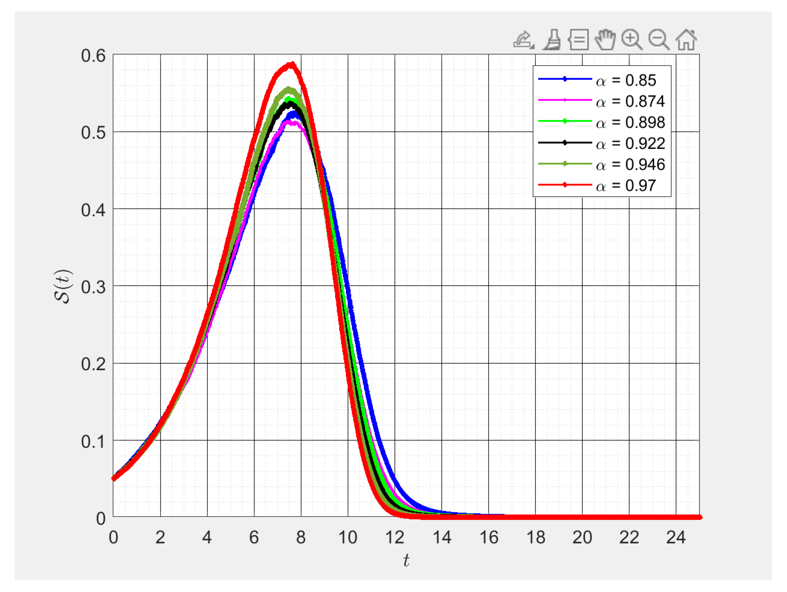
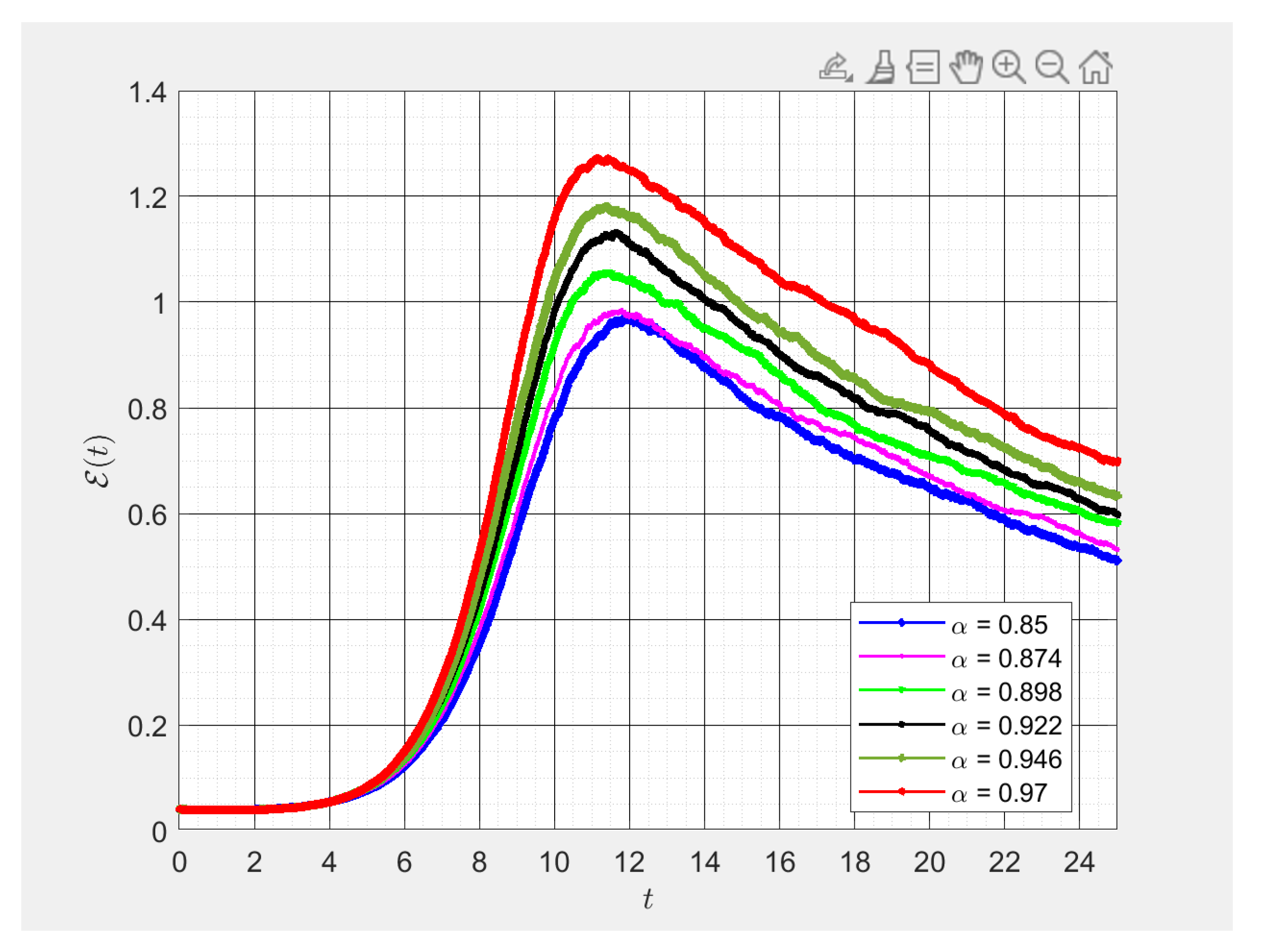
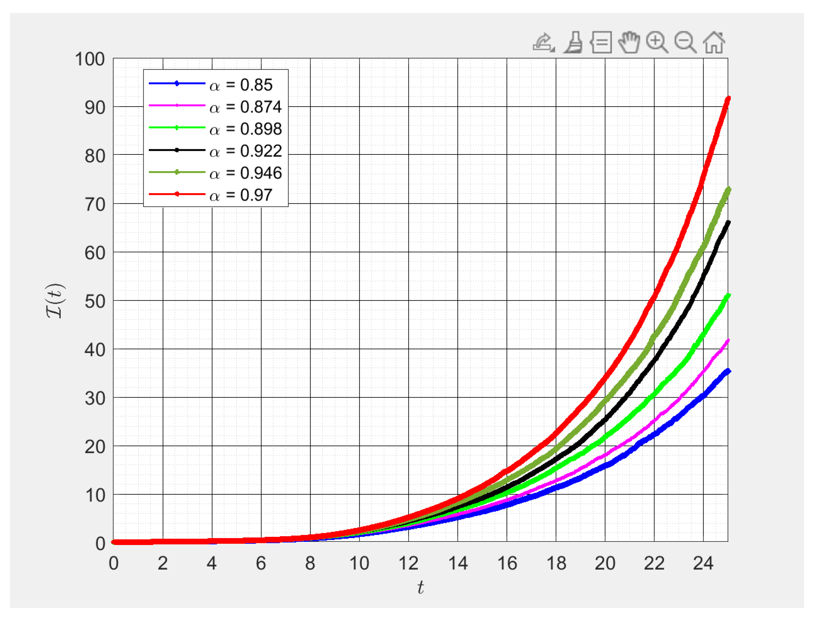
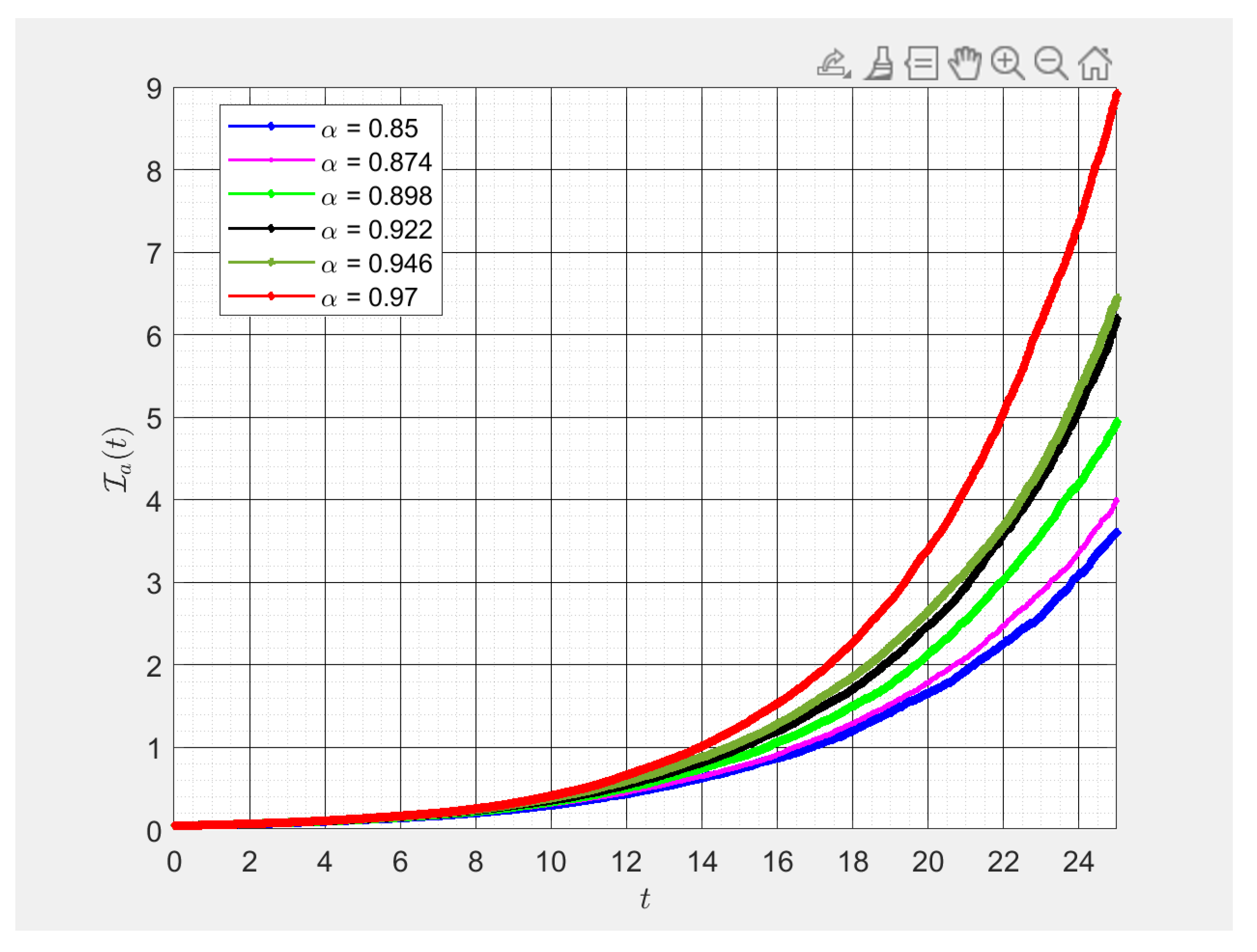
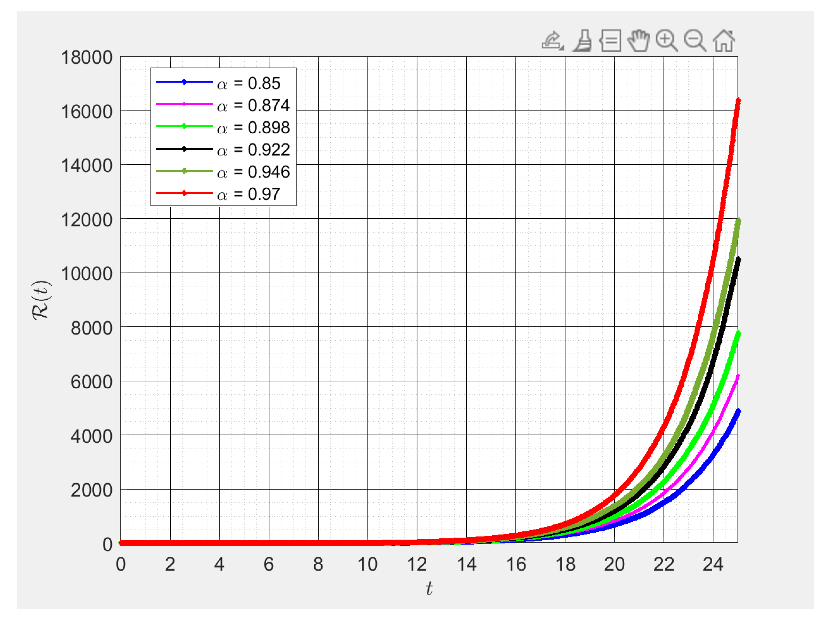
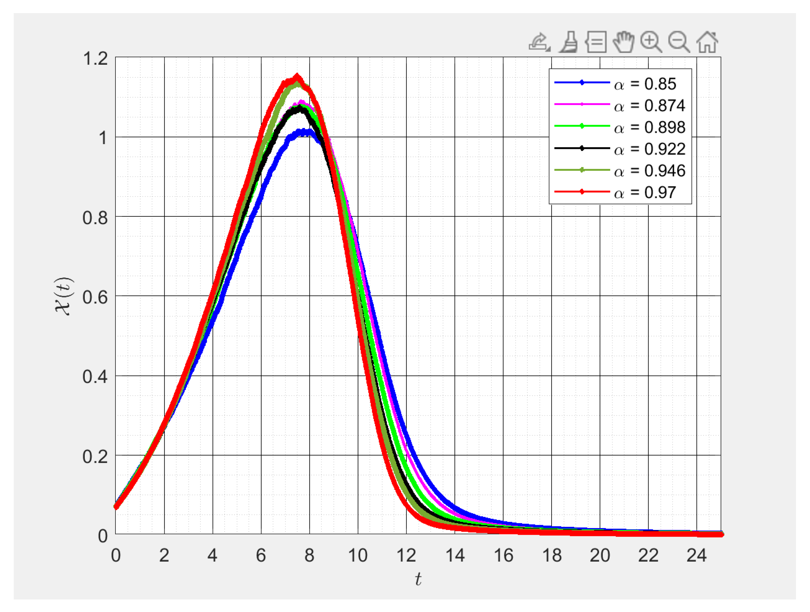
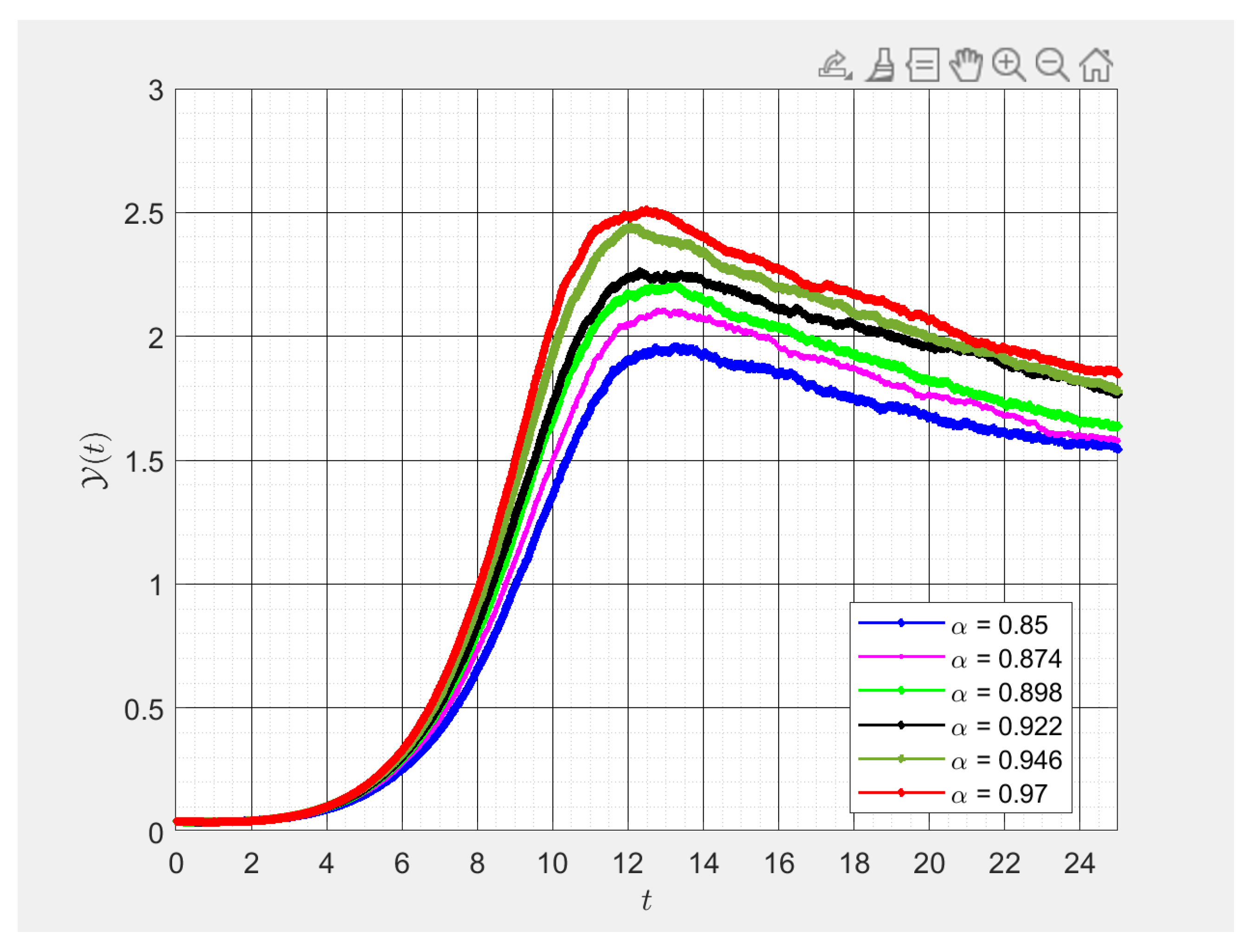
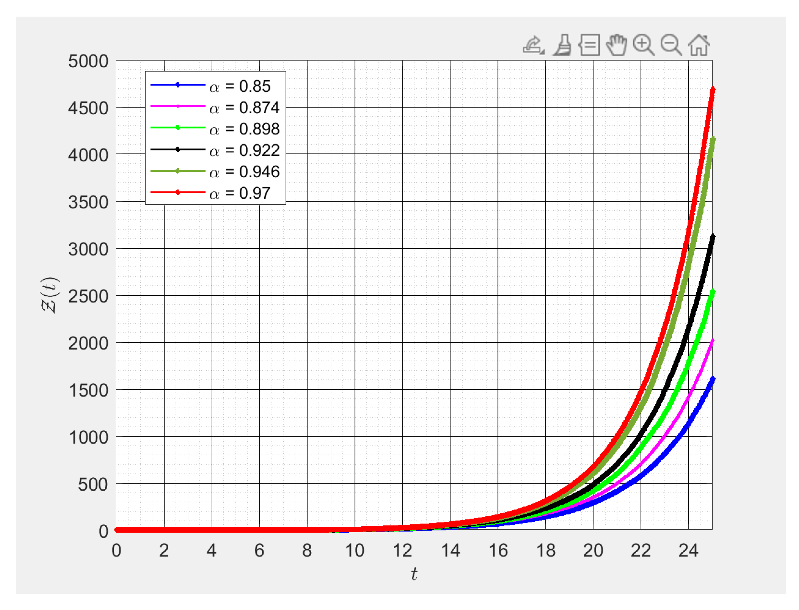
6. Numerical Simulation

Using the previously proposed numerical scheme, we provide some numerical simulations in this part for various values of fractional orders.
The MATLAB ODE15s function was used to progress the numerical approximation for the fractional Chikungunya model, as stated by Equation (83) in time. On a digital ALIENWARE computer with a Core i7, 11th generation, 32 GB RAM, 512 GB SSD, and an 8 GB Nvidia GTX 1070 graphics card, all simulations were run using the MATLAB 2021a package.
In addition, we present the treatment of patients with Chikungunya under the fractional derivatives in the sense of the A B operator. First, let us redefine the variables to be determined in the model. S ( t ) is the number of susceptible individuals in the population and the number of individuals exposed to Chikungunya is represented by E ( t ) . Then, the symptomatically infectious host is given by I ( t ) and I a represents the asymptomatically infectious hosts (proportion). R ( t ) represents the recovered hosts. X is defined for the susceptible mosquitoes. Furthermore, Y is given for exposed mosquitoes and Z is for infectious mosquitoes.
The initial conditions used in the simulation experiments are S ( 0 ) = 0.05 , E ( 0 ) = 0.05 , I ( 0 ) = 0 , I a ( 0 ) = 0.01 , R ( 0 ) = 0.001 , X ( 0 ) = 0.08 , Y ( 0 ) = 0.09 , Z = 0.02 , with time-step h = 0.01.
Considering the parameters observed in the system for a total simulation time t = 80/days, the following are given. The mosquito-to-human transmission (number of mosquito bites per human per day allowing for imperfect pathogen transmission) β 1 = 0.14 ; the human-to-mosquito transmission (per day bite rate also allowing for imperfect pathogen transmission) value β 2 is 0.40. The hosts that develop symptoms value is ϕ = 0.97 ; the host latent period (from ‘infected’ to ‘infectious’, days) is 1 λ 1 = 0.50 ; 1 λ 2 = 0.50 is the value of the mosquito latent period (from ‘infected’ to ‘infectious’, days). The value of γ = 0.25 is the host recovery rate (per day); 1 ω 1 = 0.25 is the host pre-patient period (from ‘infected’ to symptoms development, days); and the mosquito life span (days) is μ = 0.05 .
First of all, the values of variables are given at different time levels and the behavior of S ( t ) , E ( t ) , I ( t ) , I a ( t ) , R ( t ) , X , Y , Z are presented in Figure 1, Figure 2, Figure 3, Figure 4, Figure 5, Figure 6, Figure 7 and Figure 8 for h = 0.01, and at different instances of fractional order α ( 0 , 1 ] . In order to simulate the dynamic behavior of the fractional Chikungunya model as shown in Figure 1, Figure 2, Figure 3, Figure 4, Figure 5, Figure 6, Figure 7 and Figure 8, numerical experiments were carried out for various values of the parameters. Beginning with the numerical method in Equation (75), we allowed the fractional values α and used fixed parameters as stated above. Figure 1, Figure 2, Figure 3, Figure 4, Figure 5, Figure 6, Figure 7 and Figure 8 illustrate the dynamic impacts for various values of α . When α = 0.85 , both the susceptible and infected population grew, but as α 1 , they rapidly declined. This implies that a decrease in the parameter α led to an increase in the populations that were vulnerable and infected.
Remark 2.
Although there are still concerns regarding the accuracy of computer simulation models, they are being utilized more frequently to help public health research and policy. This articles goal was to examine the fundamentals and procedures for validating population-based disease simulation models.
We created a thorough methodology for evaluating the simulation models of chronic diseases in populations. We created a list of suggestions for assembling the proof of model believability based on the review.
Examining the model development process, the model’s performance, and the caliber of decisions made using the model provided evidence of the model’s legitimacy. Current recommendations do not sufficiently address several significant concerns in model validation. A thorough assessment of various data sources, graphical model representation, computer programming, model calibration, model-to-model comparisons, sensitivity analysis, and prediction validity are some of these concerns. The function of the model determines the part that external data play in model validation (e.g., decision analysis versus prediction). The techniques for comparing the caliber of judgments based on various models require more study.

7. Conclusions

The complicated transmission of the Chikungunya virus within a target population was modeled in this work using fractional differential and integral operators. We provided a thorough analysis supporting the presence and particular system of remedies for each scenario using Caputo, Caputo-Fabrizio, and Atangana-Baleanu fractional derivatives. This was accomplished by confirming the circumstances under which the Lipschitz quadratic and linear growth properties held true. Using a numerical technique based on the Newton polynomial, each model was handled differently. To examine the impact of the fractional order, certain simulations were provided.
One limitation of this approach is that when α = 1 , the accuracy of the fractional order operators with singular kernels may result in a subpar accuracy. Accordingly, from this perspective, the numerical solutions of high-dimensional partial fractional differential equations (PFDEs) require a lot of computations, but the numerical issues are not the primary justifications for using non-singular memory operators rather than those with power-law memories. We must find a solution to the computational issues if the physical model predicts power-law memory, but replacing it with other memories (such as operators with non-singular memories) is wrong and goes against the physics that the model was based on. Using the Caputo-Fabrizio fractional derivative with a non-singular kernel, we were able to solve these challenges.
The controllability and stability of the studied system should be considered as a future work. Given that the system can also be extended through a stochastic model using fractional Brownian motion, the optimal controllability using the numerical simulation will be more advanced in future work. In the studied system, we have considered the system components in the fractional order form. One can consider the fractional order system but not component-wise.

Author Contributions

Methodology, S.J. and D.N.C.; Software, S.J. and D.N.C.; Formal analysis, S.J. and D.N.C.; Investigation, S.J. and D.N.C. All authors contributed equally in this research work. All authors have read and agreed to the published version of the manuscript.

Funding

This research received no external funding.

Data Availability Statement

Not applicable. No practical data have been used for this research.

Conflicts of Interest

The authors declare no conflict of interest.

References

  1. Atangana, A.; Jain, S. A new numerical approximation of the fractal ordinary differential equation. Eur. Phys. J. Plus 2018, 133, 37. [Google Scholar] [CrossRef]
  2. Atangana, A. Fractal-fractional differentiation and integration: Connecting fractal calculus and fractional calculus to predict complex system. Chaos Soliton Fract. 2017, 102, 396–406. [Google Scholar] [CrossRef]
  3. Atangana, A.; Jain, S. Models of fluid flowing in non-conventional media: New numerical analysis. Discret. Contin. Dyn. Syst. Ser. S 2020, 13, 467. [Google Scholar] [CrossRef]
  4. Ben Makhlouf, A. A novel finite time stability analysis of nonlinear fractional-order time delay systems: A fixed point approach. Asian J. Control. 2022, 24, 3580–3587. [Google Scholar] [CrossRef]
  5. Shymanskyi, V.; Sokolovskyy, Y. Finite element calculation of the linear elasticity problem for biomaterials with fractal structure. Open Bioinform. J. 2021, 14, 114–122. [Google Scholar] [CrossRef]
  6. Lu, J.-G. Chaotic dynamics of the fractional order Ikeda delay system and its synchronization. Chin. Phys. 2006, 15, 301. [Google Scholar]
  7. Bhalekar, S. Stability and bifurcation analysis of a generalized scalar delay differential equation. Chaos Interdiscip. J. Nonlinear Sci. 2016, 26, 084306. [Google Scholar] [CrossRef]
  8. Jain, S. Numerical Analysis for the Fractional Diffusion and Fractional Buckmaster’s Equation by Two Step Adam- Bashforth Method. Eur. Phys. J. Plus 2018, 133, 19. [Google Scholar] [CrossRef]
  9. Abidemi, A.; Owolabi, K.M.; Pindza, E. Modelling the transmission dynamics of Lassa fever with nonlinear incidence rate and vertical transmission. Phys. A Stat. Mech. Appl. 2022, 597, 127259. [Google Scholar] [CrossRef]
  10. Podlubny, I. Fractional Differential Equations; Academic Press: New York, NY, USA, 1999. [Google Scholar]
  11. Diethelm, K. A fractional calculus based model for the simulation of an outbreak of dengue fever. Nonlinear Dyn. 2013, 71, 613–619. [Google Scholar] [CrossRef]
  12. Pitolli, F.; Sorgentone, C.; Pellegrino, E. Approximation of the Riesz-Caputo derivative by cubic splines. Algorithms 2022, 15, 69. [Google Scholar] [CrossRef]
  13. Izadi, M.; Srivastava, H.M. A discretization approach for the nonlinear fractional logistic equation. Entropy 2020, 22, 1328. [Google Scholar] [CrossRef]
  14. Samko, S.G.; Kilbas, A.A.; Marichev, O.I. Fractional Integrals and Derivatives, Theory and Applications, Edited and with a Foreword by S. M. Nikolskiı, Translated from the 1987 Russian Original; Revised by the authors; Gordon and Breach Science Publishers: Yverdon, Switzerland, 1993. [Google Scholar]
  15. Caputo, M.; Fabrizio, M. A new definition of fractional derivative without singular kernel. Prog. Fract. Differ. Appl. 2015, 1, 73–85. [Google Scholar]
  16. Atangana, A.; Dumitru, B. New fractional derivatives with nonlocal and non-singular kernel: Theory and application to heat transfer model. Therma Sci. 2016, 20, 763–769. [Google Scholar] [CrossRef]
  17. Yakob, L.; Clements, A.C. A mathematical model of chikungunya dynamics and control: The major epidemic on Reunion Island. PLoS ONE 2013, 8, e57448. [Google Scholar] [CrossRef] [PubMed]
  18. Atangana, A.; Araz, S.I. New numerical method for ordinary differential equations: Newton polynomial. J. Comput. Appl. Math. 2020, 372, 112622. [Google Scholar] [CrossRef]
Figure 1. Various values of fractional order numerical results of S ( t ) . This figure was obtained using A B -fractional derivative for different fractional values of alpha. By changing values of alpha slightly, we studied the transmission rates of those susceptible to the pathogen with respect to time in days, S ( t ) .
Symmetry 15 00952 g001
Figure 2. Various values of fractional order numerical results of E ( t ) . This figure was obtained using A B -fractional derivative for different fractional values of alpha. By changing values of alpha slightly, we studied the transmission rates of those exposed to the pathogen with respect to time in days, E ( t ) .
Symmetry 15 00952 g002
Figure 3. Various values of fractional order numerical results of I ( t ) . This figure was obtained using A B -fractional derivative for different fractional values of alpha. By changing values of alpha slightly, we studied the transmission rates of those symptomatically infected with respect to time in days, I ( t ) .
Symmetry 15 00952 g003
Figure 4. Various values of fractional order numerical results of I a ( t ) . This figure was obtained using A B -fractional derivative for different fractional values of alpha. By changing values of alpha slightly, we studied the transmission rates of those asymptomatically infected with respect to time in days, I a ( t ) .
Symmetry 15 00952 g004
Figure 5. Various values of fractional order numerical results of R ( t ) . This figure was obtained using A B -fractional derivative for different fractional values of alpha. By changing values of alpha slightly, we studied the transmission rates of the recovered host with respect to time in days, R ( t ) .
Symmetry 15 00952 g005
Figure 6. Various values of fractional order numerical results of X ( t ) . This figure was obtained using A B -fractional derivative for different fractional values of alpha. By changing values of alpha slightly, we studied the transmission rates of susceptible mosquitoes with respect to time in days, X ( t ) .
Symmetry 15 00952 g006
Figure 7. Various values of fractional order numerical results of Y ( t ) . This figure was obtained using A B -fractional derivative for different fractional values of alpha. By changing values of alpha slightly, we studied the transmission rates of exposed mosquitoes with respect to time in days, Y ( t ) .
Symmetry 15 00952 g007
Figure 8. Various values of fractional order numerical results of Y ( t ) . This figure was obtained using A B -fractional derivative for different fractional values of alpha. By changing values of alpha slightly, we studied the transmission rates of infected mosquitoes with respect to time in days, Z ( t ) .
Symmetry 15 00952 g008
Disclaimer/Publisher’s Note: The statements, opinions and data contained in all publications are solely those of the individual author(s) and contributor(s) and not of MDPI and/or the editor(s). MDPI and/or the editor(s) disclaim responsibility for any injury to people or property resulting from any ideas, methods, instructions or products referred to in the content.

