Time Series Analysis Based on Informer Algorithms: A Survey

Abstract

Long series time forecasting has become a popular research direction in recent years, due to the ability to predict weather changes, traffic conditions and so on. This paper provides a comprehensive discussion of long series time forecasting techniques and their applications, using the Informer algorithm model as a framework. Specifically, we examine sequential time prediction models published in the last two years, including the tightly coupled convolutional transformer (TCCT) algorithm, Autoformer algorithm, FEDformer algorithm, Pyraformer algorithm, and Triformer algorithm. Researchers have made significant improvements to the attention mechanism and Informer algorithm model architecture in these different neural network models, resulting in recent approaches such as wavelet enhancement structure, auto-correlation mechanism, and depth decomposition architecture. In addition to the above, attention algorithms and many models show potential and possibility in mechanical vibration prediction. In recent state-of-the-art studies, researchers have used the Informer algorithm model as an experimental control, and it can be seen that the algorithm model itself has research value. The informer algorithm model performs relatively well on various data sets and has become a more typical algorithm model for time series forecasting, and its model value is worthy of in-depth exploration and research. This paper discusses the structures and innovations of five representative models, including Informer, and reviews the performance of different neural network structures. The advantages and disadvantages of each model are discussed and compared, and finally, the future research direction of long series time forecasting is discussed.

1. Introduction

In recent years, long series time forecasting (LSTF) has become a widely used technique in various fields, including weather forecasting [1], stock market analysis [2], medical diagnosis [3], traffic prediction [4], defect detection [5], vibration analysis [6], action recognition [7], and anomaly detection [8]. The Transformer algorithm model was introduced by the Google team in 2017 [9] and has since replaced the Long Short-Term Memory (LSTM) algorithm model [10] as one of the most popular neural network prediction models. The Transformer algorithm model has been shown to outperform the LSTM algorithm model in terms of both accuracy and computational efficiency. However, researchers have found that the Transformer algorithm model still faces several challenges that limit the direct application to long series time forecasting problems, such as secondary spatio-temporal complexity, high memory usage, and inherent limitations of the encoder–decoder architecture.

To address these challenges, researchers have developed an efficient algorithmic model called Informer for long series time forecasting, which is based on the Transformer model [11]. The Informer model employs the ProbSparse self-attention mechanism, which achieves $\mathrm{O}(L/\log L)$ time complexity and enhances sequence dependency alignment, resulting in more reliable performance. Several new algorithmic models have been developed to improve the Transformer model and enhance the attention and encoder–decoder architecture of the Informer model. As the Transformer model still suffers from loose coupling, Shen et al. proposed the TCCT algorithmic model in 2021 [12]. They introduced the Cross Stage Partial Attention (CSPAttention) mechanism, which combines Cross Stage Partial Network (CSPNet) with the self-attention mechanism, resulting in a 30% reduction in computational cost and a 50% reduction in memory usage. Whereas this improvement solves the issue of loose coupling, some limitations of the Transformer model remain, such as ignoring the potential correlation between sequences and the encoder–decoder structure’s limited scalability during the optimization algorithm. To address these limitations, Su et al. proposed the Adaptive Graph Convolutional Network for a Transformer-based Long Sequence Time-Series Forecasting (AGCNT) algorithmic model in 2021 [13]. The AGCNT model captures the correlations between sequences in multivariate long series time forecasting problems without causing memory bottlenecks.

The application of methods based on the Transformer algorithm model has led to significant improvements in long series time forecasting, but these models are still plagued by issues such as high computational cost and the inability to capture a global view of the time series. To overcome these challenges, several new algorithmic models have been proposed recently. For instance, Zhou et al. introduced the FEDformer algorithm model in 2022 [14], which leverages trend decomposition to capture a global view of the time series by incorporating seasonal trends. The Autoformer algorithm model proposed by Wu et al. [15] takes a different approach, with a deep decomposition architecture that extracts more predictable components from complex time series and enables targeted attention to reliable temporal dependencies that were previously undetected. Additionally, Liu et al. presented the Pyraformer algorithm model in 2022 [16], which employs a pyramidal self-attention mechanism to capture temporal features of different scales and reduces computation time and memory consumption while performing high-precision single-step and long time multi-step forecasting tasks. Finally, in 2022, Razvan-Gabriel Cirstea et al. introduced the Triformer algorithm model [17], which uses the patch attention algorithm to replace the original attention algorithm, proposes a triangular shrinkage module as a new pooling method, and employs a modeling approach for lightweight variables to enable the model to obtain features between different variables.

Various methods have been developed to predict mechanical vibration faults using models associated with the Informer algorithm [6]. Predicting vibration faults can allow for the early detection of equipment failures, the identification of the failure location, and the determination of the type of failure in the case of serious equipment failures. The time series prediction of equipment vibration is a valuable research direction in predicting failure and the remaining service life of electromechanical equipment. By applying fault prediction based on vibration data of electromechanical equipment to the manufacturing and operation and maintenance process of various products, the loss of electromechanical equipment can be avoided, resulting in cost savings and loss reduction. The time series prediction of motor-bearing vibration involves analyzing the historical data of its components to determine the possibility of future failure. Yang et al. [6] applied the Informer algorithm model to motor-bearing vibration prediction and proposed a random search-based time series prediction method for optimizing the Informer algorithm model. By optimizing the Informer and using a stochastic search to optimize the model parameters, the authors achieved better algorithmic performance in the time series prediction of motor bearing vibration.

During the process of developing new models, it is evident that the Informer algorithm model is built upon the Transformer algorithm model with innovative improvements. Nonetheless, it holds significant research value and innovative significance, making it a typical algorithmic model with architecture and core algorithmic principles worth exploring and studying in depth. The rapid emergence of subsequent models is influenced to some extent by the Informer model.

In view of this, this paper presents an overview of related algorithmic models such as Informer. The contributions of this paper are summarized as follows:

• In this paper, the principle of the Informer algorithm model, related structure, and attention algorithm are restated in detail, and the advantages and shortcomings of the informer algorithm model are analyzed.
• In this paper, we kindly discuss in detail the innovations and improvements in the model structure of several other advanced algorithmic models (including TCCT, Autoformer, FEDformer, Pyraformer, and Triformer)
• We study an overview of the attentional algorithm structure and innovations for each model, and we also provide a critical analysis of the models and attention mechanisms that were studied and summarize the advantages and disadvantages of each model.
• In this paper, we compare and analyze each algorithm model with the informer algorithm model, showing the feasibility of the attention mechanism and related models such as the informer algorithm model and making predictions and outlooks on future research directions.

2. Background of Informer Algorithm Model and Architecture

This section introduces the inception and fundamental structure of the Informer algorithm model. Initially, the problem of long series time forecasting is defined, followed by a novel analysis and exploration of the Informer algorithm model. A review of the framework treatment is also provided.

2.1. Basic Forecasting Problem Definition

LSTF utilizes the long-term dependencies between spatial and temporal domains, contextual information, and inherent patterns in data to improve predictive performance. Recent research has shown that the Informer algorithm model and its variants have the potential to further enhance this performance. In this section, we begin by introducing the input and output representations, as well as the structural representation, in the LSTF problem.

In the scrolling prediction setting with a fixed-size window, the input is represented by ${\chi }^t=\{x_1^t,\dots ,x_{L_x}^t|{\mathrm{x}}_i^t\in {ℝ}^{d_x}\}$, while the output is the predicted corresponding sequence $Y^t=\{y_1^t,\cdots ,y_{Ly}^t|y_i^t\in R^{d_y}\}$ at time t. The LSTF problem is capable of handling longer output lengths than previous works, and its feature dimensionality is not limited to the univariate case ($d_y$ ≥ 1).

The encoder–decoder operation is mainly carried out through a step-by-step process. Many popular models are designed to encode the input ${\chi }^t$ as a hidden state $H^t$ and decode the output representation $Y^t$ from $H^t=\{h_1^t,\cdots ,h_{Lh}^t\}$. The inference involves a stepwise process called “dynamic decoding”, in which the decoder computes a new hidden state $h_{k+1}^t$ from the previous state $h_k^t$ and other necessary outputs at step k, and then predicts the sequence $y_{k+1}^t$ at step (k + 1).

2.2. Informer Architecture

This section presents an overview of the refined Informer algorithm model architecture designed by Zhou et al. [11] The Informer algorithm model is an improvement on the transformer, and its structure is similar to the transformer in that it is a multi-layer structure made by stacking informer blocks. Informer modules are characterized by a ProbSparse multi-head self-focus mechanism, an encoder–decoder structure.

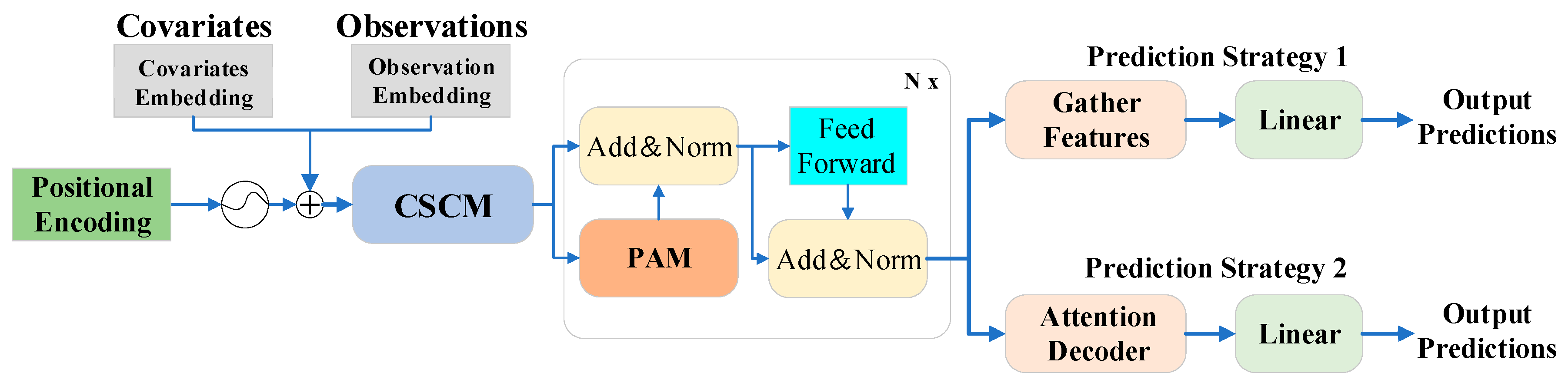
The following figure shows the basic architecture of the Informer algorithm model. The schematic diagram in the left part of the figure shows the encoder receiving a large number of long sequence inputs with the proposed ProbSparse self-attention instead of the canonical self-attention. The green trapezoid is a self-attention distillation operation that extracts the dominant attention and greatly reduces the network size. The layer-stacked copies increase the robustness. The decoder in the right part of the figure receives the long sequence input, fills the target element with zero, measures the weighted attentional composition of the feature map, and immediately predicts the output element in a generative manner.

The model successfully improves the predictive power of the LSTF problem and validates the potential value of the transformer family of models in capturing individual long-range dependencies between the output and the input of long time series. The ProbSparse self-attention mechanism is successfully proposed to effectively replace the canonical self-attention. The $\mathrm{O}(L/\log L)$ time complexity and $\mathrm{O}(L/\log L)$ memory footprint of dependency alignment is achieved. The research article presents the self-attention extraction operation to control the attention fraction in the stacked layers and significantly reduce the total space complexity to $\mathrm{O}(L/\log L)$, which helps the model to receive long-range inputs. Meanwhile, researchers proposed a generative decoder to obtain long sequence outputs with only one forward step while avoiding the cumulative error expansion in the inference stage.

In the original transformer model, the canonical self-attention is defined based on tuple inputs, which are queries, keys, and values, and it performs the scaled dot product for $A(Q,K,V)=\mathit{Softmax}(Q{K}^{\top }/\sqrt{d})V$, where $Q\in {ℝ}^{LQ\times d}$,$K\in {ℝ}^{LK\times d}$,$V\in {ℝ}^{LV\times d}$ and d represent the input dimensions. To further discuss the self-attention mechanism, let $q_i,k_i,v_i$ represent the i-th row in Q, K, and V, respectively. Following the formulas in references [18,19], the attention of the i-th query is defined as a kernel smoother in the form of probability:

$$A(q_i,K,V)={\displaystyle \sum _j\frac{k(q_i,k_j)}{{\sum }_{l}k(q_i,k_i)}}{v}_j=E_{p(k_j|q_i)}[v_j]$$

(1)

where $p(k_j|q_i)=k(q_i,k_j)/{\sum }_{l}k(q_i,k_l)$ and $k(q_i,k_j)$ choose the asymmetric index kernel $exp(q_i{k}_j{}^{\top }/\sqrt{d})$. The output obtained by self-attention is mainly derived by combining the values after calculating the probability $p(k_j,q_i)$. Additionally, it requires quadratic dot product computation and memory. Additionally, its need for quadratic dot product computation and $\mathrm{O}(L_Q{L}_K)$ memory is the main drawback of self-attention in the transformer.

The self-attention mechanism is an improved attention model, which is simply summarized as a self-learning representation process. Moreover, the computational overhead of self-attention is quadratically correlated with sequence length, which leads to low computational efficiency, slow computational speed and high training costs of the Transformer model, and the excessive computational overhead also makes the application of the model difficult; the processing capability of long sequence data is thus limited in the Transformer model.

Therefore, studying variants of the self-attention mechanism to achieve an efficient Transformer has become an important research direction. The Informer algorithm model has been preceded by equally many proposals to reduce memory usage and computation and increase efficiency.

Sparse Transformer [20] combines row output and column input, where sparsity comes from separated spatial correlations. LogSparse Transformer [21] notes the circular pattern of self-attention and makes each cell focus on its previous cell in exponential steps. Longformer [22] extends the first two works to more complex sparse configurations.

However, they use the same strategy to deal with each multi-headed self-attention, a mode of thinking that makes it difficult to develop novel and efficient models. In order to reduce memory usage and improve computational efficiency, researchers first qualitatively evaluated the learned attention patterns of typical self-attention in the Informer algorithm model, i.e., a few dot product pairs contribute major attention, while others produce very little attention.

The following discussion focuses on the differences between the differentiated dot products. From the above equation, the attention of the i-th query to all keys is defined as the probability $p(k_j|q_i)$, and the output is its combination with the value V. The dominant dot product pair encourages the attention probability distribution of the corresponding query to be far from a uniform distribution. If $p(k_j|q_i)$ is close to a uniform distribution, which is $p(k_j|q_i)=1/L_K$, then the result of the self-attention calculation becomes a numerically small sum of V values, which is redundant for the input. Therefore, the “similarity” between distributions p and q can be used to distinguish “important” queries. The “similarity” can be measured by the Kullback–Leibler scatter:

$$KL(q||p)=\ln {\displaystyle \sum }_{l=1}^{L_k}{e}^{q_i{k}_l{}^{\top }/\sqrt{d}}-\frac{1}{L_k}{\displaystyle \sum }_{j=1}^{LK}{q}_i{k}_j^{\top }/\sqrt{d}-\ln L_k$$

(2)

removing the constants, the sparsity measure for the i-th query is defined as the following equation:

$$M(q_i,K)=\ln {\displaystyle \sum }_{j=1}^{LK}{e}^{\frac{q_i{k}_j{}^{\top }}{\sqrt{d}}}-\frac{1}{LK}{\displaystyle \sum }_{j=1}^{LK}\frac{q_i{K}_j{}^{\top }}{\sqrt{d}}$$

(3)

where the first term is the Log-Sum-Exp of all keys $q_i$ and the second term is their arithmetic mean. If the i-th query obtains a larger $M(q_i,K)$, it has a more diverse attention probability p and is likely to contain dominant dot product pairs in the head fields of the long-tailed self-attention distribution. Additionally, ProbSparse self-attention is achieved by allowing each key to focus on only u primary queries:

$$A(Q,K,V)=Softmax(\frac{\overline{Q}{K}^{\top }}{\sqrt{d}})V$$

(4)

where $\overline{Q}$ is a sparse matrix of the same size as q, which contains only the Top-u queries under the sparse metric $M(q,K)$. Under the control of a constant sampling factor c, $u=c\cdot \ln L_Q$ is set in such a way that ProbSparse self-attention only needs to compute $\mathrm{O}(\ln L_Q)$ dot products for each query-key lookup, and memory usage per layer is kept at $\mathrm{O}(L_K\ln L_Q)$.

In the multi-head perspective, this attention generates different sparse query-key pairs for each head, thus avoiding severe information loss. Additionally, to address the quadratic complexity problem and the fact that LSE operations have potential numerical stability, researchers proposed an empirical approximation for efficiently obtaining query sparsity measures.

Lemma 1. 

For each $q_i\in R^{\mathrm{d}}$in the set K as well as $k_j\in R^{\mathrm{d}}$, the bound is the following equation:

$$\ln L_K\le M(q_i,K)\le ma{x}_j\{q_i{k}_j^{\top }/\sqrt{d}\}-\frac{1}{L_K}{\displaystyle \sum }_{j=1}^{LK}\{q_i{k}_{{}_j}^{\top }/\sqrt{d}\}+\ln L_K$$

(5)

This equation also holds when $q_i\in K$, starting with Lemma 1, and the maximum mean measure is proposed as the following equation [11]:

$$M(q_i,K)=\underset{j}{max}\{\frac{q_i{k}_j{}^{\top }}{\sqrt{d}}\}-\frac{1}{L_K}{\displaystyle \sum }_{j=1}^{L_K}\frac{q_i{k}_j{}^{\top }}{\sqrt{d}}$$

(6)

randomly selected $U=LK ln LQ$ dot product pairs are used to compute $M(q_i,K)$, meaning that the other pairs are filled with zeros, from which the sparse Top-u is selected as $\overline{Q}$. The maximum operator in $M(q_i,K)$ is less sensitive to zero values and is numerically stable. In practice, the input lengths of queries and keys are usually equivalent in the self-attention computation, which means that $L_Q=L_K=L$. This makes the total time complexity and space complexity of ProbSparse self-attention $\mathrm{O}(L\ln L)$.

2.3. Encoder

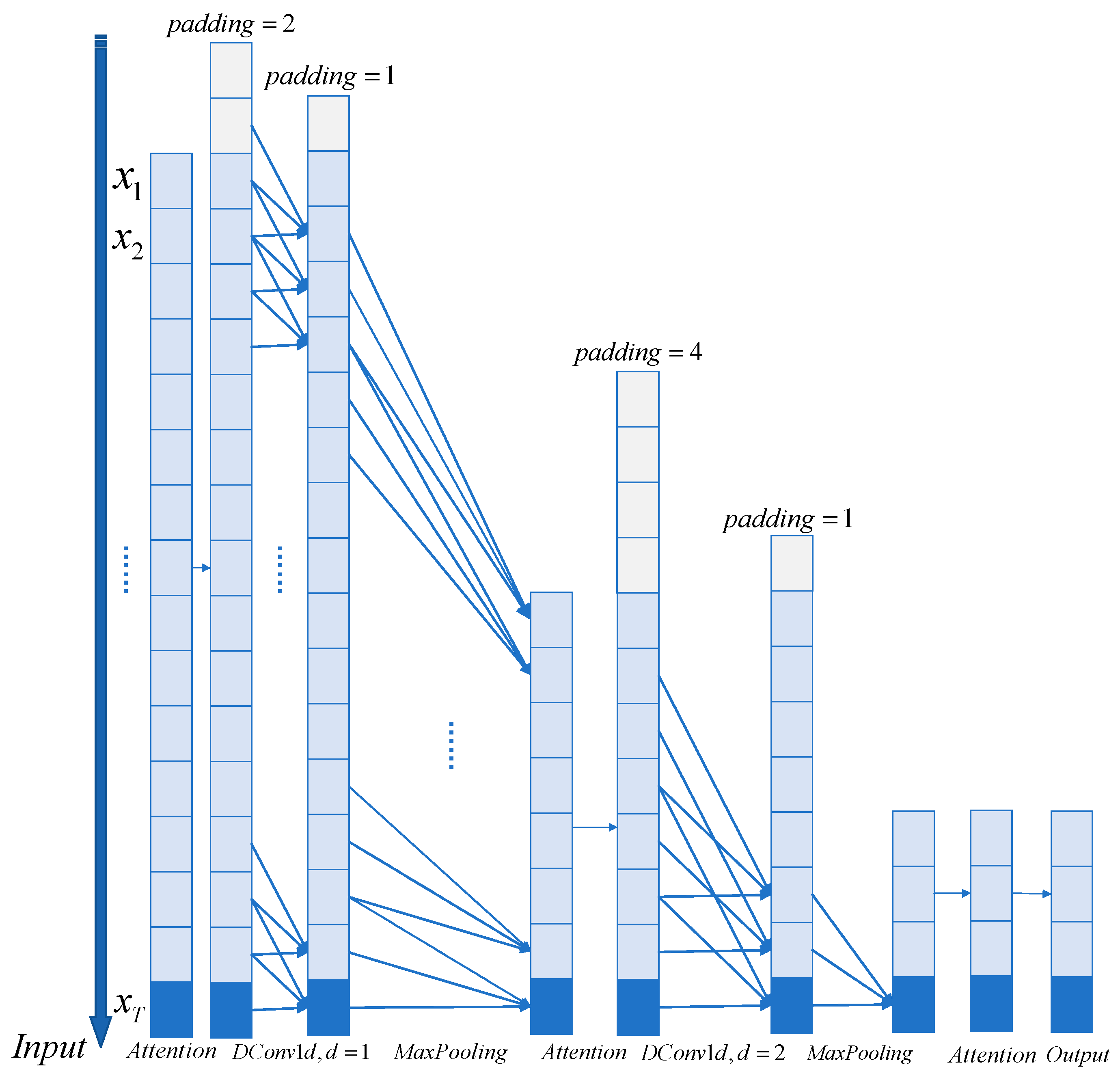
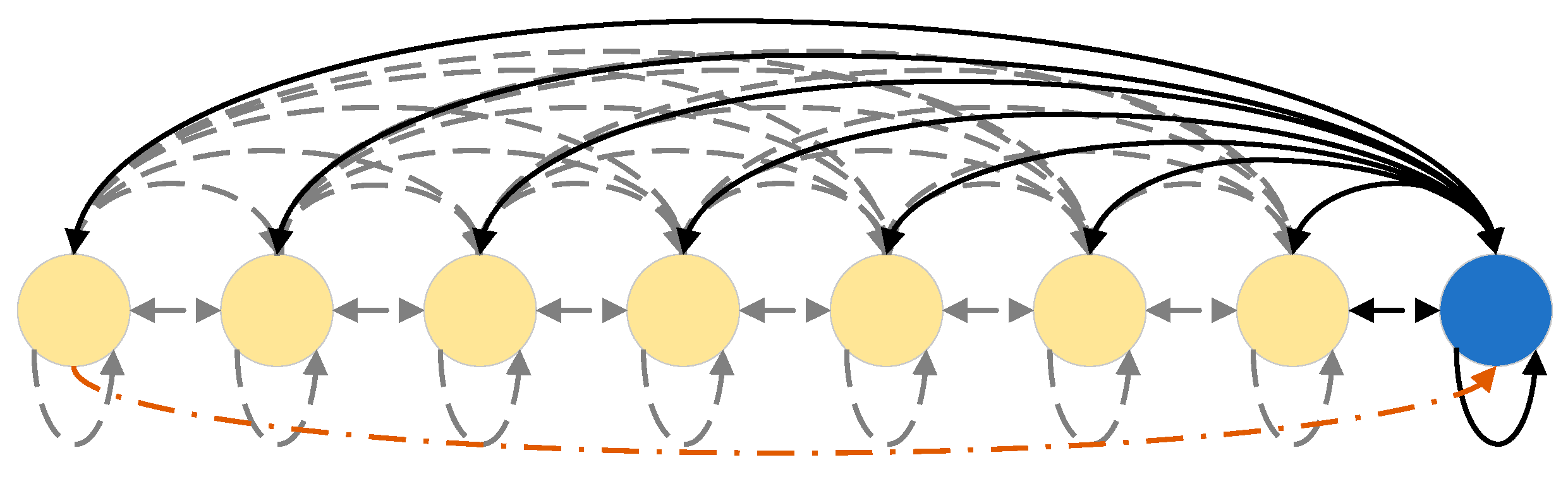
In Figure 1, it can be seen that Encoder receives a large number of long sequence inputs, while the model uses ProbSparse self-attention instead of self-attention in Transformer. The green trapezoid is the extraction operation of self-attention, which mainly extracts the dominant attention and drastically reduces the amount of computation and memory occupied. Additionally, the layer-stacked copies increase the robustness.

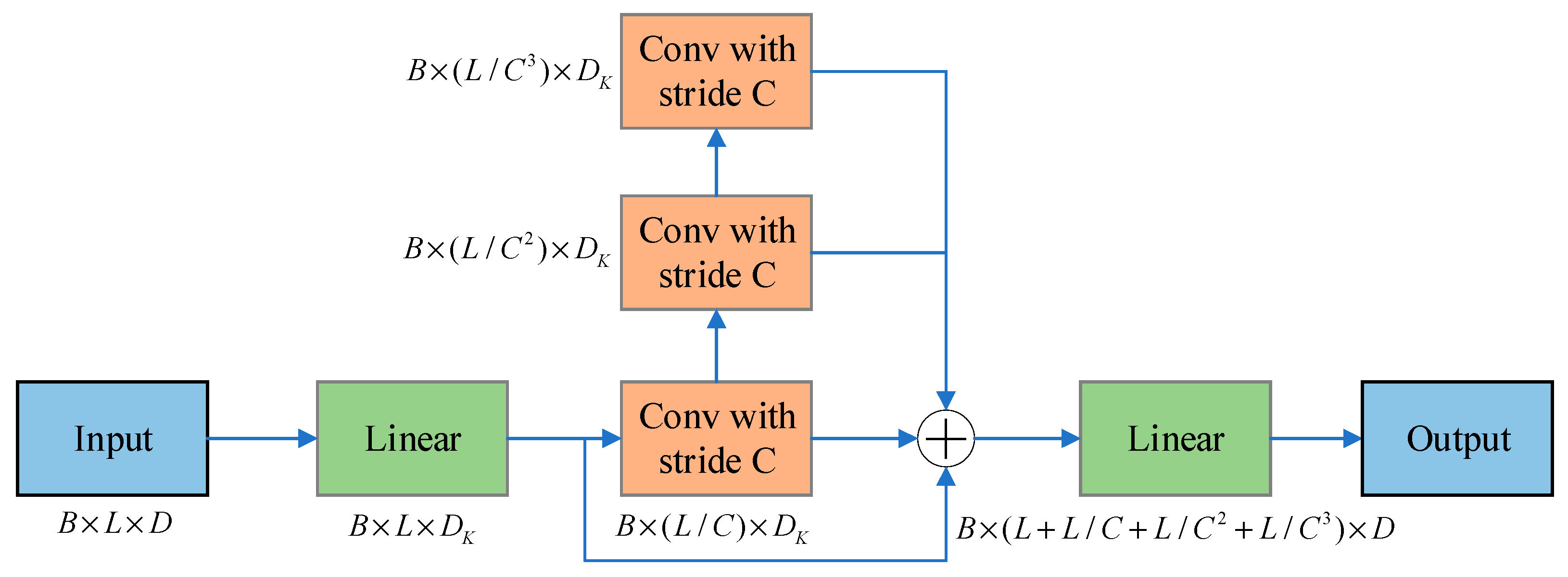
The encoder is designed to extract robust remote dependencies for long sequence inputs. After the input representation, the t-th sequential input $X^t$ has been shaped into a matrix $X_{en}^t\in {ℝ}^{L_x\times d_{model}}$, and the following diagram shows the structure of a single stack of the encoder:

In the above figure, the horizontal stack represents one of the copies of a single encoder. The one presented in Figure 2 is the main stack that receives the entire input sequence. The second stack then acquires half of the slices of the input, and the subsequent stacks are repeated. The red layer is a dot product matrix, and the red layer is reduced in cascade by performing self-attention extraction on each layer. The output of the encoder is then performed by connecting the feature maps of all stacks.

As a natural consequence of the ProbSparse self-attention mechanism, the feature maps of the encoder have redundant combinations of values V. The distillation operation is used to assign weights to the values with dominant features and to produce a new self-attention feature map at the next level. This operation substantially prunes the temporal dimension of the input, and the n-head weight matrix of the attention block is seen in Figure 2. Inspired by the expansion convolution [23], the “distillation” process advances from the j-th layer to the (j + 1) layer, as follows:

$$X_{j+1}^t=\mathrm{MaxPool}\left(\mathrm{EIU}\left(\mathrm{Conv}1\mathrm{d}\left({\left[X_j^t\right]}_{AB}\right)\right)\right)$$

(7)

where ${[\cdot ]}_{AB}$ represents the attention block. It contains the multi-headed ProbSparse self-attention and the basic operations, where $Conv1d(\cdot )$ performs a one-dimensional convolutional filter in the time dimension using the $\mathrm{ELU}(\cdot )$ activation function [24].

The Researchers add a maximum pooling layer spanning 2 and down-sample $X^t$ into half of its slices after stacking one layer, which reduces the overall memory usage to $\mathrm{O}((2-ϵ)L\log L)$, where $ϵ$ is a small number. To enhance the robustness of the extraction operation, copies of the main stack is also constructed using halved inputs, and the number of self-focused extraction layers is gradually reduced by performing one layer at a time, aligning their output dimensions and joining the outputs of all stacks to obtain the final hidden representation of the encoder.

2.4. Decoder

A standard decoder structure is used in the Informer algorithm model, which consists of two identical multi-headed attention layers. However, the generative inference is used to mitigate the speed plunge in long series time forecasting. The decoder takes the long sequence input, fills the target elements with zeros, measures the weighted attention composition of the feature map, and immediately predicts the output elements in a generative manner.

In Figure 1, the decoder receives the long sequence input, fills the target elements with zero, measures the weighted attention composition of the feature map, and instantly predicts the output elements in a generative style. Regarding the implementation principle of the decoder, the following vectors are first provided to the decoder:

$$X_{de}^t=\mathrm{Concat}\left(X_{token}^t,X_0^t\right)\in {ℝ}^{(L_{\mathrm{token}}+L_y)\times d_{model}}$$

(8)

where $X_{token}^t\in R^{L_{\mathrm{token}}\times d_{model}}$ is the start marker and $X_0^t\in R^{Ly\times d_{model}}$ is a placeholder for the target sequence (setting the scalar to 0). By setting the masked dot product to negative infinity, a multi-headed masked attention mechanism is applied in the ProbSparse self-attention calculation. It prevents each position from paying attention to the upcoming position, thus avoiding the autoregression. The fully connected layer obtains the final output, whose size $d_{\mathrm{y}}$ depends on whether univariate or multivariate prediction is performed.

Regarding the problem of long output length, the original transformer has no way to solve this problem; it is dynamically output with the same cascade output as the RNN-like model, which cannot handle long sequences. A start token in the dynamic decoding process of NLP is a great trick [25], especially for the pre-training model stage, and the concept is extended in the Informer algorithm model for the long series time forecasting problem by proposing a generative decoder for the long sequence output problem, that is, generating all the predicted data at once. The Q, K, and V values in the first masked attention layer are obtained by multiplying the embedding values from the decoder input by the weight matrix, while the Q values in the second attention layer are obtained by multiplying the output of the previous attention layer by the weight matrix, and the K and V values are obtained by multiplying the output of the encoder by the weight matrix.

2.5. Informer Algorithm Model Values

The ProbSparse self-attention mechanism in the Informer algorithm model can achieve $\mathrm{O}(L/\log L)$ in terms of time complexity and memory usage, making a large adjustment relative to transformer in terms of time complexity and memory, while the self-attention mechanism highlights the cascade layer input by halving the dominant attention and efficiently handle overly long input sequences. The proposed generative decoder performs one forward operation on long sequences instead of prediction by stepping, which greatly improves the inference speed of long sequence forecasting.

First, the improved attention mechanism reduces the complexity and memory, but there is still room for improvement in reducing the complexity and memory consumption; second, although the efficiency is improved, there are still problems with the backward and forward time dependence, which leads to some errors between the prediction results and the actual results, and the accuracy still needs to be improved. Finally, the structure of the generative decoder is too simple, with few innovations, and similar to that of the transformer, so there is still room for structural adjustment.

3. Relevant Model Development

3.1. TCCT Algorithmic Model

Time series forecasting is crucial for a wide range of practical applications. models such as Informer are superior in handling such problems, especially long series time input (LSTI) and long series time forecasting (LSTF) problems. To improve the efficiency and enhance the localization of this class of models, some researchers have combined the models with CNNs [26,27,28] to varying degrees. However, their combinations are loosely coupled and do not take full advantage of CNNs, whereas three architectures of TCCT algorithmic models can be a good solution to the above problem. This section focuses on three TCCT algorithm model architectures. These architectures not only enhance the local performance of the Transformer, but also enhance the learning capability of the Transformer and reduce the computational cost and memory usage. It can also handle other time series forecasting models similar to Transformer algorithm models.

This section also elaborates the principle of the passthrough mechanism. Its main purpose is to obtain finer-grained information by connecting the feature maps of self-attention blocks at different scales. It is similar to CNN and features pyramids commonly used in image processing. As it extends the feature graph, it improves the prediction performance of the Transformer model.

3.1.1. Dilated Causal Convolutions

Stacking multiple self-attention blocks facilitates the extraction of deeper feature maps but introduces more time and space complexity. To further reduce memory usage, the Informer algorithm model uses a self-attention distilling operation. the Informer algorithm model uses a convolutional layer and a maximum pooling layer to trim the input length between every two self-attention blocks. A kernel of step size 1 and a convolutional layer of size 3 follow the previous self-attention block to make the features more aware of local contextual information. A kernel of step size 2 and a max-pooling layer of size 3 are then used to privilege locally dominant features and provide a smaller but more focused feature map for the latter self-attention block. However, canonical convolutional layers have two main drawbacks when applied to time series prediction.

First, it can only review the history of linear size as the depth of the network grows. In the Informer algorithm model, it mainly deals with long series time forecasting problem, but it is also not powerful enough in dealing with very long series. As the computational cost grows, the advantages of stacking self-attention blocks with canonical convolutional layers are gradually overshadowed by the disadvantages, which may lead to repetitive and meaningless computations due to the limited perceptual field. Second, the canonical convolution layer in the informer algorithm model does not consider the time perspective, which will inevitably lead to future information leakage in time series prediction and reduce the time perception field.

To address the above problem, the solution is inspired by TCN and replaces the canonical convolution with a dilated causal convolution to obtain the growth of the feeling field. More precisely, for the i-th convolutional layer after the i-th self-attention block, the dilated causal convolution operation C with kernel size k on element $x_n\in {ℝ}^d$ of sequence $\mathcal{X}\in {ℝ}^{L\times d}$ is defined as:

$$C(x_n)=\left[\begin{array}{c}{x}_n\\ x_{n-i}\\ ⋮\\ x_{n-(k-1)\times i}\end{array}\right]W^{d\times d^{\prime }}$$

(9)

where $d^{\prime }$ is the output dimension, where the number i is also used as the expansion factor. The filter of the i-th expanded causal convolution layer skips ${(2}^{i-1}-1)$ elements between two adjacent filter taps.

Due to the nature of causality, each element x at time t of the sequence is only convolved with the element at or before t, ensuring that there is no information leakage in the future. When i = 1, the dilated causal convolution degenerates to a normal causal convolution.

An illustration of a self-attention network stacked with three self-attention blocks and using the dilated causal convolutional layer of kernel 3 is provided in Figure 3. Researchers stacked such self-attention networks with three self-attention blocks that are connected to the dilated causal convolution layer and the max-pool layer. It can be seen that the application of the dilated causal convolutions layer can bring a wider feeling field and avoid future information leakage.

Dilated causal convolution uses padding only at the front end of time to prevent the leakage of future information. Even with only two convolutional layers, the output perceptual field of the network in this figure is significantly larger than the one above. Therefore, stacking more self-attention blocks, the gap will be larger and, therefore, the two networks will perform better. In addition to this, the application of Dilated causal convolution will only incur a negligible amount of computational cost and memory usage.

3.1.2. TCCT Architecture and Passthrough Mechanism

Feature pyramids are commonly used to extract features in computer vision and CNNs. A similar concept can be applied to Transformer-based networks. According to the studies related to the Yolo series of target detection CNN networks [29,30], a passthrough mechanism is proposed to obtain feature maps from the earlier networks and merge them with the final feature maps to obtain finer-grained information.

In Transformer-based networks, a passthrough mechanism is used to merge feature maps of different scales. Assuming that the encoder stacks n self-focused blocks, each self-focused block will produce a feature map. The k-th (k = 1, 2…, n) feature map has length $L/2^{k-1}$ and dimensionality d. Assume that CSPAttention and dilation causal convolution have been applied to this encoder. In order to connect all feature maps of different scales, the k-th feature map is equivalently partitioned by length into $2^{n-1}$ feature maps of length $L/2^{n-1}$. In this way, all feature maps can be connected by dimension.

However, the tandem graph has dimension $(2^n-1)\times d$. Therefore, a transition layer needs to be employed to ensure that the entire network outputs feature maps are of the appropriate dimension. The above problem can be solved by stacking three self-attention blocks and using the TCCT algorithm model architecture, as shown in Figure 4.

The passthrough mechanism works similarly to the full distillation operation in the Informer algorithm model. However, the Informer algorithm model with full distillation requires as many encoders as the number of self-attention blocks of the main encoder, whereas the Informer algorithm model with straight-through mechanism requires only one encoder.

This is despite the fact that the Informer algorithm model with full distillation has encoders with decreasing input length and it draws more attention from the model to the later timing data. For example, assuming that Informer stacks k encoders, the first half of the input sequence exists only in the main encoder, and conversely, the $1/2^{k-1}$ of the later part of the input sequence exists in each individual encoder. The passthrough mechanism has no such deficiency. More importantly, the passthrough mechanism imposes almost no additional computational cost on the Informer algorithm model, whereas the Informer algorithm model with full distillation operation incurs considerable additional computational cost due to its multi-coder architecture.

3.1.3. Transformer with TCCT Architectures

CSPAttention, passthrough mechanism architecture, and dilated causal convolution [12] all work seamlessly with canonical Transformer, LogTrans, Informer, and other time series algorithm prediction models. A simple example of collaboration with the Informer algorithm model is shown in the Figure 5, and a detailed encoder example can be seen in the final figure in this section. Note that the Informer algorithm model in the figure below has only one encoder, which means that it does not use the full distillation operation but replaces it with a passthrough mechanism.

In the above figure within the blue trapezoid are encoders stacked with three probabilistic sparse CSPAttention blocks which replace the probabilistic sparse self-attention blocks from before the figure, employing an inflated causal convolutional layer instead of the canonical convolutional layer, together with a max pooling layer in the green trapezoid being used to connect every two self-attention blocks. Without adding additional encoders, all three feature mappings of the output of the three self-attention blocks are fused and then transitioned to the final output of appropriate size. The right panel makes no significant changes compared to informer’s decoder, except that the masked probability sparse self-attention blocks are replaced by masked probability sparse CSPAttention blocks.

Based on the Informer architecture, other similar architectures can easily work with the TCCT algorithm model architecture. For example, to combine the TCCT algorithm model architecture with the LogTrans algorithm model, the masked probabilistic sparse self-attention block in the above figure will be replaced by the masked LogSparse self-attention block, and the other architectures remain unchanged.

In Figure 6, each CSPAttention block is combined with Probsparse self-attention, which is a typical architecture of Informer. Additionally, between each two CSPAttention blocks, a connection is made using a dilated causal convolutional layer and a maxpooling layer. The output feature map of the previous self-attention block is propagated through these two layers and reduced to half the length, reflecting the original Informer while expanding the perceptual field. The three feature maps of the output of the three self-attention blocks are also fused by a passthrough mechanism to obtain more fine-grained information. Finally, a transition layer is added to export the feature mappings of appropriate dimensions to the decoder.

3.1.4. TCCT Algorithm Model Value

The concept of tightly coupled convolutional Transformer and three TCCT algorithm model architectures proposed by shen et al. [12] improves the predictive power of models such as Informer for time series prediction. Especially, the CSPAttention is designed to reduce the computational cost and memory usage of the self-attention mechanism without degrading the prediction accuracy. In addition, the application of dilated causal convolution enables models such as Informer to obtain exponential receptive field growth. A passthrough mechanism is also employed to help individual models obtain more fine-grained information. Individual and extensive experiments on real data sets show that all three TCCT algorithm model architectures can improve model performance in time series forecasting in different ways.

3.2. Autoformer

This section introduces the structure and principles of the Autoformer algorithm model and disassembles and analyzes the deep decomposition architecture of Autoformer as well as the encoder–decoder architecture.

The related research based on the Transformer prediction model is to capture the inter-moment dependence through the self-attention mechanism, thus making some progress on the temporal sequence prediction. However, in long series time forecasting, the complex temporal patterns in long sequences make it difficult for the attention mechanism to discover reliable temporal dependencies, and the Transformer-based model has to use a sparse form of the attention mechanism to cope with the quadratic complexity, and the processing approach adopted in the above studies creates a bottleneck in information utilization. To break through the above problems, researchers propose an algorithmic model called Autoformer based on the basic Transformer architecture, which innovates the original sequence decomposition as a traditional method of preprocessing and proposes a deep decomposition architecture where the model is able to decompose more predictable components from complex temporal patterns.

3.2.1. Deep Decomposition Architecture

The encoder eliminates the long-term trend cycle component through the series decomposition block and focuses on seasonal pattern modeling. The decoder progressively accumulates the trend component extracted from the hidden variables. The past seasonal information of the encoder is utilized through encoder–decoder auto-correlation, and the architecture of the AutoFormer algorithm model is shown in Figure 7.

Time series decomposition is the decomposition of time series into several components. Each component represents a class of potential time patterns, such as seasonal, trend-cyclical terms. Due to the unpredictability of the future in forecasting problems, the past series are usually decomposed first and then forecasted separately. However, this causes the prediction results to be limited by the decomposition effect and ignores the interactions between the future components. The deep decomposition architecture embeds sequence decomposition as an internal unit of the Autoformer algorithm model in the encoder–decoder. In the prediction process, the model alternates between prediction result optimization and sequence decomposition, which means that the trend term and the period term are gradually separated from the hidden variables to achieve progressive decomposition.

3.2.2. Encoder

The input to the model uses the second half of the encoder input as input to provide the most recent information, represented by ${\mathcal{X}}_{\mathrm{en}\frac{I}{2}:I}$. In Figure 7, the series decomposition block is based on the idea of a sliding average, smoothing the period term and highlighting the trend term. The model input formula is the following formula:

$$\begin{array}{l}{\mathcal{X}}_t=\mathrm{AvgPool}(\mathrm{Padding}(\mathcal{X}))\\ {\mathcal{X}}_{\mathrm{s}}=\mathcal{X}-{\mathcal{X}}_t\end{array}$$

(10)

where $\mathcal{X}$ is the hidden variable to be decomposed, ${\mathcal{X}}_t$ and ${\mathcal{X}}_{\mathrm{s}}$ are the trend term and the period term, respectively, and the above equation is written as:

$${\mathcal{X}}_s,{\mathcal{X}}_t=\mathrm{SeriesDecomp}(\mathcal{X})$$

(11)

the above sequence decomposition unit is embedded between Autoformer layers. The input to the encoder part is the time step ${\mathcal{X}}_{\mathrm{en}}\in {ℝ}^{I\times d}$ of the past i-th. As a decomposition structure in Figure 7, the input contains both the season part ${\mathcal{X}}_{\mathrm{de}\mathrm{s}}\in {ℝ}^{(\frac{I}{2}+O)\times d}$ and the trend recurrence part ${\mathcal{X}}_{\det }\in {ℝ}^{(\frac{I}{2}+O)\times d}$. Each initialization part consists of two parts: a decomposition from the second half of the encoder input ${\mathcal{X}}_{\mathrm{en}}$, of length $\frac{I}{2}$, to provide the most recent information, and a placeholder of length $O$ filled by a scalar. The format is as follows:

$$\begin{array}{l}{\mathcal{X}}_{ens},{\mathcal{X}}_{ent}=\mathrm{SeriesDecomp}({\mathcal{X}}_{\mathrm{en}\frac{I}{2}:I})\\ {\mathcal{X}}_{\mathrm{de}\mathrm{s}}=\mathrm{Concat}({\mathcal{X}}_{\mathrm{ens}},{\mathcal{X}}_0)\\ {\mathcal{X}}_{\det }=\mathrm{Concat}({\mathcal{X}}_{\mathrm{ent}},{\mathcal{X}}_{\mathrm{Mean}}),\end{array}$$

(12)

where ${\mathcal{X}}_{\mathrm{ens}},{\mathcal{X}}_{\mathrm{ent}}\in {ℝ}^{\frac{I}{2}\times d}$ denote the seasonal and trend cycle components of ${\mathcal{X}}_{\mathrm{en}}$, respectively, and ${\mathcal{X}}_0,{\mathcal{X}}_{\mathrm{Mean}}\in {ℝ}^{O\times d}$ denote the mean and zero placeholder of ${\mathcal{X}}_{\mathrm{en}}$, respectively.

As shown in Figure 7, the encoder focuses on seasonal component modeling. The output of the encoder contains past seasonal information and uses it as crossover information to help the decoder refine the prediction results. Assume that there are N encoder layers. The overall equation for the l-th encoder layer is summarized as ${\mathcal{X}}_{\mathrm{en}}^l=\mathrm{Encoder}({\mathcal{X}}_{\mathrm{en}}^{l-1})$. Details are as follows:

$$\begin{array}{l}{S}_{en}^{l,1},\_=\mathrm{SeriesDecomp}(\mathrm{Auto}\text{-}\mathrm{Correlation}({\mathcal{X}}_{\mathrm{en}}^{l-1})+{\mathcal{X}}_{\mathrm{en}}^{l-1}),\\ S_{en}^{l,2},\_=\mathrm{SeriesDecomp}(\mathrm{FeedForward}(S_{\mathrm{en}}^{l,1})+S_{\mathrm{en}}^{l,1}),\end{array}$$

(13)

where “$\_$“ is the part of the trend that is eliminated. ${\mathcal{X}}_{en}^l={\mathcal{S}}_{en}^{l,2},l\in \{1,\cdots ,N\}$ denotes the output of the l-th encoder layer and ${\mathcal{X}}_{\mathrm{en}}^0$ is the embedded ${\mathcal{X}}_{\mathrm{en}}^{}$. $S_{en}^{l,i},i\in \{1,2\}$ denotes the seasonal component after the i-th sequence decomposition block of the L-th layer, respectively.

The ${\mathcal{X}}_{\mathrm{en}\frac{I}{2}:I}$ signal involved above is used as input, and the results before and after the auto-correlation are summed up and then enter the sequence decomposition module. The encoder part of the Autoformer algorithm model is more concerned with the seasonal decomposition part, and the trend decomposition part is removed. The encoder wants to optimize the cycle transformation learning process, and through the encoding process, the results before the encoding are summed up with the results after the encoding, and then go through the sequence decomposition in order to reduce the computational complexity and computational time.

3.2.3. Decoder

The decoder contains two components: an accumulation structure for the trend cycle component and a stacked auto-correlation mechanism for the seasonal component. Each decoder layer contains internal autocorrelation and encoding–decoding auto-correlation, refining the predictions and using past seasonal information, respectively. The decoder structure is shown in Figure 7. Note that the model extracts potential trends from intermediate hidden variables during the decoder process, allowing the Autoformer algorithm model to progressively refine the trend predictions and eliminate confounding information for cycle-based dependence in auto-correlation discovery. Assume that there are m decoder layers. Using the latent variable ${\mathcal{X}}_{\mathrm{en}}^N$ of the encoder, the equations for the l-th decoder layer can be generalized to ${\mathcal{X}}_{\mathrm{de}}^l=\mathrm{Decoder}({\mathcal{X}}_{\mathrm{de}}^{l-1},{\mathcal{X}}_{\mathrm{en}}^N)$. The decoder can be formalized as:

$$\begin{array}{l}{S}_{\mathrm{de}}^{l,1},{\mathcal{T}}_{\mathrm{de}}^{l,1}=\mathrm{SeriesDecomp}(\mathrm{Auto}\text{-}\mathrm{Correlation}({\mathcal{X}}_{\mathrm{de}}^{l-1})+{\mathcal{X}}_{\mathrm{de}}^{l-1}),\\ S_{\mathrm{de}}^{l,2},{\mathcal{T}}_{\mathrm{de}}^{l,2}=\mathrm{SeriesDecomp}(\mathrm{Auto}\text{-}\mathrm{Correlation}(S_{\mathrm{de}}^{l,1},{\mathcal{X}}_{\mathrm{en}}^N)+S_{\mathrm{de}}^{l,1}),\\ S_{\mathrm{de}}^{l,3},{\mathcal{T}}_{\mathrm{de}}^{l,3}=\mathrm{SeriesDecomp}(\mathrm{FeedForward}(S_{\mathrm{de}}^{l,2})+S_{\mathrm{de}}^{l,2}),\\ \hspace{1em}\hspace{1em}{\mathcal{T}}_{de}^l={\mathcal{T}}_{de}^{l-1}+{\mathcal{W}}_{l,1}\cdot {\mathcal{T}}_{de}^{l,1}+{\mathcal{W}}_{l,2}\cdot {\mathcal{T}}_{de}^{l,2}+{\mathcal{W}}_{l,3}\cdot {\mathcal{T}}_{de}^{l,3},\end{array}$$

(14)

where ${\mathcal{X}}_{\mathrm{de}}^l={\mathcal{S}}_{\mathrm{de}}^{l,3},l\in \{1,\cdots ,M\}$ denotes the output of the l-th decoder layer. ${\mathcal{X}}_{\mathrm{de}}^0$ is embedded from ${\mathcal{X}}_{\mathrm{des}}$, which is used for depth transformation, and ${\mathcal{T}}_{de}^0={\mathcal{X}}_{\det }$ is used for accumulation. $S_{\mathrm{de}}^{l,2},{\mathcal{T}}_{\mathrm{de}}^{l,2},i\in \{1,2,3\}$ denotes the seasonal component and trend cycle component of the l-th layer after the i-th sequence decomposition block, respectively. ${\mathcal{W}}_{l,i},i\in \{1,2,3\}$ denotes the projector of the i-th extracted trend ${\mathcal{T}}_{\mathrm{de}}^{l,i}$. The final projection is the sum of the components of the two refined decompositions, as ${\mathcal{W}}_S\ast {\mathcal{X}}_{de}^M+{\mathcal{T}}_{de}^M$, where ${\mathcal{W}}_S$ is the projection of the depth-transformed seasonal component ${\mathcal{X}}_{de}^M$ into the target dimension.

3.2.4. Autoformer Algorithm Model Architecture Value

To address the problem of complex time patterns in long series time forecasting that are difficult to handle and computationally efficient, Wu et al. [15] proposed the Autoformer algorithm model based on the deep decomposition architecture and auto-correlation mechanism. FFT is a widely used algorithm [31,32] that still plays its core value today, and the Autoformer algorithm model combining the encoder–decoder mechanism is improved and updated. By progressive decomposition and sequence-level concatenation, the long series time forecasting efficiency is significantly improved.

At the same time, the Autoformer algorithm model shows excellent long series time forecasting results in the five mainstream fields of energy, transportation, economy, meteorology, and disease, and the model has good effect robustness with strong application landing value.

3.3. FEDformer

Although models such as Informer have made relevant structural improvements to the transformer that significantly improve long series time forecasting results, they still suffer from high computational cost and the inability to capture a global view of the time series, among other problems. This section focuses on the encoder and decoder architectures in the FEDformer algorithmic model. The algorithmic features of frequency domain operations and the use of expert mixture blocks for seasonal trend decomposition are explained.

3.3.1. Application of Neural Networks in Frequency Domain Operations

The work carried out by the researchers differs slightly from other long time forecasting algorithms in that it mainly uses neural networks for frequency domain operations and takes the approach of using Fourier’s algorithm to represent the information in the time series for time series forecasting [14]. In frequency domain operations, simply retaining all frequency components may result in less accurate representations because many of the high-frequency changes in the time series are due to noisy inputs. Retaining only the low-frequency components may also be unsuitable for series prediction since some trend changes in the time series represent significant events. Instead, maintaining a compact representation of the time series using a small number of selected Fourier components can make the computation efficient, which is crucial for long series time forecasting. In contrast, the FEDformer algorithm model takes the approach of representing the time series by randomly selecting a fixed number of Fourier components (both high- and low-frequency), which, in layman’s terms, means performing a Fourier transform on each time series.

The researchers verify the feasibility and necessity of the FEDformer algorithm model by relevant calculations in the process of proposing the algorithm model. A time series is first transformed into a vector $X_i(t)$→$a_i={(a_{i,1},\cdots ,a_{i,d})}^T\in {ℝ}^d$ and then obtained by substituting all the transformed vectors into a matrix $A={(a_1,a_2,\cdots ,a_m)}^{\top }\in {ℝ}^{m\times d}$, each row corresponding to a different time series and each column corresponding to a different Fourier component. Although using all the Fourier components can better preserve the historical information in the time series, it may lead to the overfitting of the historical data, which can lead to poor predictions of future signals. Therefore, a subset of Fourier components needs to be chosen that is small enough to avoid the overfitting problem on the one hand and capable of preserving most of the historical information on the other. Consequently, researchers proposed to select s components (s < d) uniformly and randomly from d Fourier components. Specifically, $i_1<i_2<\cdots <i_s$ is used to denote the randomly selected components. The matrix $S\in {\{0,1\}}^{s\times d}$ is established. If $i=i_k$, then $S_{i,k}=1$, otherwise $S_{i,k}=0$. Thus, the representation of the multivariate time series becomes $A^{\prime }=A{S}^{\top }\in {ℝ}^{m\times s}$.

To measure the ability of ${\mathrm{A}}^{\prime }$ to preserve information from $\mathrm{A}$, each column vector of $\mathrm{A}$ is projected into a subspace consisting of the column vectors in ${\mathrm{A}}^{\prime }$. The result matrix after projection is denoted by $P_{{\mathrm{A}}^{\prime }}(\mathrm{A})$, where $P_{{\mathrm{A}}^{\prime }}(\cdot )$ denotes the projection operator. The error between $\mathrm{A}$ and $P_{{\mathrm{A}}^{\prime }}(\mathrm{A})$ is expected to be small if ${\mathrm{A}}^{\prime }$ retains most of the information of $\mathrm{A}$. Let ${\mathrm{A}}_{\mathrm{k}}$ represent the approximation of $\mathrm{A}$ using the first k largest single-value decompositions of $\mathrm{A}$. If the Fourier component s of random sampling is of the order of $k^2$, then $|\mathrm{A}-{\mathrm{P}}_{{\mathrm{A}}^{\prime }}\left(\mathrm{A}\right)|$ and $|\mathrm{A}-{\mathrm{A}}_{\mathrm{k}}|$ are close.

For multivariate time series, the matrix $\mathrm{A}$ corresponding to the Fourier transform tends to exhibit low-rankness because the univariate variables in a multivariate time series not only depend on their past values, but the variables have dependencies on each other and share similar frequency components. Therefore, a subset of randomly selected Fourier components can properly represent information in the Fourier matrix $\mathrm{A}$. Similarly, wavelet canonical polynomials [33], such as Lejeune polynomials, obey the property of restricted isometry and can be used for information capture in time series. Compared to Fourier bases, wavelet representations are more effective in capturing the local structure in time series and therefore more efficient in certain prediction tasks.

Additionally, the researchers found that in various cases, the distribution of model inputs and true values differed significantly, leading to inaccurate predicted values of the model. To solve this problem, the FEDformer algorithm model is structured to reduce the differences in the distributions of the inputs and outputs by decomposing the periodic trend terms; to better capture the global characteristics of the time series, the seasonal trend decomposition is incorporated, and, inspired by the seasonal trend decomposition and distribution analysis, the depth of the Informer architecture and the transformer architecture are updated based on the original decomposition architecture, including frequency enhanced block (FEB), frequency enhanced attention (FEA) connecting encoder and decoder, and mixture of expert decomposition blocks (MOEDecomp).

3.3.2. FEDformer Algorithm Model Architecture

FEDformer’s encoder uses a multilayer structure ${\mathcal{X}}_{en}^l=\mathrm{Encoder}\left({\mathcal{X}}_{en}^{l-1}\right)$. n denotes the output of the l-th encoding layer, ${\mathcal{X}}_{en}^0$ is the embedded history sequence, formalized as follows:

$$\begin{array}{l}{S}_{en}^{l,1},\_=MOEDecomp(FEB({\mathcal{X}}_{en}^{l-1})+{\mathcal{X}}_{en}^{l-1}),\\ S_{en}^{l,2},\_=MOEDecomp(\mathrm{FeedForward}(S_{en}^{l,1})+S_{en}^{l,1}),\\ {\mathcal{X}}_{en}^l={\mathcal{S}}_{en}^{l,2}\end{array}$$

(15)

where $S_{en}^{l,i},i\in \{1,2\}$ denotes the seasonal component after the i-th decomposition block of the first and second layers, respectively. For the FEB module, it has two different versions (FEB-f and FEB-w) which are implemented by the discrete Fourier transform (DFT) and discrete wavelet transform (DWT) mechanisms, respectively, and can replace the self-attention blocks.

The decoder also uses a multi-layer structure: ${\mathcal{X}}_{de}^l,{\mathcal{T}}_{de}^l=\mathrm{Decoder}\left({\mathcal{X}}_{en}^{l-1},{\mathcal{T}}_{de}^{l-1}\right)$. Where A denotes the output of the layer l decoder, $\mathrm{Decoder}(\cdot )$ is formalized as follows:

$$\begin{array}{l}{S}_{de}^{l,1},{\mathcal{T}}_{de}^{l,1}=MOEDecomp(FEB({\mathcal{X}}_{de}^{l-1})+{\mathcal{X}}_{de}^{l-1}),\\ S_{de}^{l,2},{\mathcal{T}}_{de}^{l,2}=MOEDecomp(\mathrm{FEA}(S_{de}^{l,1},{\mathcal{X}}_{en}^N)+S_{de}^{l,1}),\\ S_{de}^{l,3},{\mathcal{T}}_{de}^{l,3}=MOEDecomp(\mathrm{FeedForward}(S_{de}^{l,2})+S_{de}^{l,2}),\\ \hspace{1em}\hspace{1em}{\mathcal{X}}_{de}^l={\mathcal{S}}_{de}^{l,3},\\ \hspace{1em}\hspace{1em}{\mathcal{T}}_{de}^l={\mathcal{T}}_{de}^{l-1}+{\mathcal{W}}_{l,1}\cdot {\mathcal{T}}_{de}^{l,1}+{\mathcal{W}}_{l,2}\cdot {\mathcal{T}}_{de}^{l,2}+{\mathcal{W}}_{l,3}\cdot {\mathcal{T}}_{de}^{l,3},\end{array}$$

(16)

where ${\mathcal{S}}_{en}^{l,i},i\in \{1,2\}$ denotes the seasonal component after the i-th decomposition block of the l-th layer, respectively, and the trend component ${\mathcal{W}}_{l,i}$ denotes the mapping of the extracted i-th trend ${\mathcal{T}}_{de}^{l,i}$.

The Figure 8 shows that the FEDformer algorithm model consists of N encoders and M decoders. Frequency enhancement blocks (FEB) and frequency enhancement attention (FEA) are used for representation learning in the frequency domain. Both FEB and FEA have two forms (FEB-F&FEB-W or FEA-F&FEA-W), where -F indicates that the Fourier basis is used and -W indicates that the wavelet basis is used. Seasonal trend patterns are extracted from the input data using a mixture of decomposition blocks.

The main structure of the FEDformer algorithm model uses an encoder–decoder structure, which internally includes four sub-modules: a frequency domain learning module, a frequency domain attention module, a period-trend decomposition module, and a forward propagation module. The input goes through two MOEDecomp layers in the encoder, and the MOEDecomp module decomposes the sequence into a sequence of period and trend terms. Additionally, this decomposition is not performed only once, but also in an iterative decomposition mode. The trend term component is discarded, and the period term component is given to the next layers for learning and finally passed to the decoder. In the decoder, the encoder input passes through three MOEDecomp layers and is decomposed into periodic and trend term components, where the periodic term component is passed to the next layers for learning, where the frequency-domain correlation between the periodic term of the encoder and decoder is learned through the frequency-domain attention algorithm layer, and the trend term component is accumulated and finally added back to the periodic term to restore the original sequence.

Extracting trends in a fixed-window averaging pooling is more difficult because of the complex periodic patterns usually observed in combination with trend components on real data. To overcome such a problem, the FEDformer algorithm model adds mixture of expert decomposition blocks, which contain a set of averaging filters of different sizes, multiple trend components extracted from the input signal, and a set of data-dependent weights that combine them into a final trend. The formulation is as follows:

$${\mathrm{X}}_{\mathrm{trend}}=\mathit{Softmax}(L(x))\ast (F(x)),$$

(17)

where $F(\cdot )$ is a set of average pool filters, and $\mathit{Softmax}(L(x))$ is the weight of the trend of mixing these extractions.

3.3.3. Learning Principles for Models in the Frequency and Time Domains

The Fourier transform and the inverse Fourier transform can transform signals between each other in the time domain and the frequency domain. The general signal is sparse in the frequency domain, which means that only a few points need to be retained in the frequency domain to restore the time domain signal almost lossless. The principle and flow of FEB operation is mainly in the following order.

The input sequence on the original time domain is first projected to the frequency domain. Then, random sampling is performed in the frequency domain. This has the advantage of greatly reducing the length of the input vector and thus the computational complexity; however, this sampling must be lossy to the input information. However, it is experimentally proven that this loss has little impact on the final accuracy. This is because the general signal can be more sparsely represented in the frequency domain compared to the time domain. A large amount of information in the high-frequency part is so-called “noise”, which can often be discarded in time series prediction problems, because “noise” often represents randomly generation and is therefore difficulties in forecasting. In contrast, in the image domain, the high frequency part of the “noise” may represent picture details that cannot be ignored. In the learning phase after this, FEB uses a fully concatenated layer R as a learnable parameter. FEA, on the other hand, cross-notes the signals from the encoder and decoder in order to learn the intrinsic relationship between the two parts of the signals. The frequency domain complementation process afterwards is relative to the frequency domain sampling in the previous steps, and in order to enable the signal to be restored back to its original length, the frequency points not picked up by the sampling need to be zeroed. Finally, the signal is projected back to the time domain, and because of the complementary operation in the previous step, the signal projected back to the frequency domain is exactly the same as the previous input signal dimension.

3.3.4. FEDformer Algorithm Model Values

The FEDformer algorithm model uses a decomposed encoder–decoder overall architecture such as the Autoformer algorithm model. To improve the efficiency of subsequence-level similarity computation, the FEDformer algorithm model uses methods such as Fourier analysis. In general, the Autoformer algorithm model can be said to decompose the sequence into multiple time-domain subsequences for feature extraction, whereas the FEDformer algorithm model uses frequency transform to decompose the sequence into multiple frequency domain modes for feature extraction. In particular, instead of using selective methods in subsequence selection, It calculates the significant frequency features in the whole sequence, and this global feature gives the model better performance for long sequences.

3.4. Pyraformer

Researchers proposed the Pyraformer algorithm model based on pyramidal attention [16]. This section introduces the performance of the Pyraformer algorithm model in terms of temporal and spatial complexity as well as long-range dependencies, and also introduces and elaborates on the overall architecture of the Pyraformer model as well as the structure and principle of the encoder–decoder.

Firstly, it is known from previous studies that the Transformer can effectively capture long-range dependencies and has a maximum path length of $\mathrm{O}(1)$, but its time and space complexity is $\mathrm{O}(L^2)$. Therefore, there are many Transformer variants that have explored this drawback of high space–time complexity to some extent; for example, Informer proves the sparsity of attention and reduces the complexity from $\mathrm{O}(L^2)$ to $\mathrm{O}(L/\log L)$, but it introduces a longer maximum path length because a part of nodes far from the uniformly distributed attention fraction is selected as query nodes.

Some of the existing models are sparse Transformer models; for example, the Longformer [22] algorithm model uses a local window similar to CNN to reduce the complexity to $\mathrm{O}(AL)$, where A is the local window size, but the limited window size makes it difficult to exchange information globally. In contrast, the Reformer [34] algorithm model uses locally sensitive hashing to divide the sequence into parts, and the maximum path length of Reformer is proportional to the number of separated parts, so it also leads to the need for a large number of components to reduce the complexity, while the number of global tokens designed by ETC is G, which usually increases with L and the consequent complexity is still more than linear.

Another class is the hierarchical Transformer, and there are two main types of such methods to improve the Transformer’s ability to capture natural language hierarchies: the Multi-scale Transformer [35] and the BP-Transformer [36]. The Multi-scale Transformer uses top-down and bottom-up network structures to learn multi-scale representations of sequential data, which can appropriately reduce the complexity of the original Transformer, but still fall into $\mathrm{O}(L^2)$ complexity. In contrast, the BP-Transformer recursively divides the entire input sequence into two until the last partition contains only one token. Then, the partitioned sequence forms a binary tree, closely related to the graph. the Pyraformer algorithm also models the partitioned sequence to form a binary tree. However, the graph associated with Pyraformer can obtain a more sparsely representation, and it reduces the maximum path length while greatly reducing the time and space complexity. It is also possible to capture the gap between remote dependencies and achieve low time and space complexity.

3.4.1. Pyraformer Algorithm Model Architecture

The structure of the Pyraformer algorithm model is presented in Figure 9, where the CSCM summarizes the embedded sequences at different scales and builds a multi-resolution tree structure. PAM is then used to exchange information between nodes efficiently.

As can be seen from Figure 9, firstly, the input historical observations embedding features, global time covariates embedding features, and position encoding are summed together, which is the same as that of the long-range time series prediction model Informer. Then, the coarse-scale construction module is used to construct a multi-resolution convolution module, and the original sequence nodes under the fine scale are used to generate the parent nodes under the coarser scale, and the number of child nodes is C times that of the parent nodes, which finally forms a C-element tree at the fine and coarser scales, with the coarser scale nodes aggregating the feature information of the C child nodes in the previous layer. To further capture the temporal dependencies at different scales, the coarse and fine scale temporal node features generated by CSCM are passed into the pyramidal attention module for inter- and intra-scale information transfer among nodes based on the attention mechanism. Finally, different prediction methods are used to predict the results for single-step prediction and multi-step prediction.

3.4.2. Coarser Scale Construction Module (CSCM)

The goal of CSCM is to initialize nodes at the coarser scales of the pyramidal graph so that subsequent PAMs can exchange information among these nodes. Specifically, coarse-scale nodes are introduced from the bottom to the top by convolving the corresponding sub-nodes C(s)ℓ.

As shown in Figure 10, B in the figure is the batch size and D is the dimension of the node. Several convolutional layers with kernel size C and step size C are applied sequentially to the embedded sequence in the time dimension. A sequence of length is generated at scale s. The dimensionality of each node is reduced by a fully connected layer before feeding the sequence into the stacked convolutional layers and recovering it after all convolutions. These sequences, ranging from fine to coarse, are connected before feeding them into the PAM. Such a structure significantly reduces the number of parameters in the module and prevents overfitting.

3.5. Triformer

This section introduces the advantages of the Triformer algorithm model over other transformer models in terms of the structure and principles of the Triformer algorithm model, using long- and short-term forecasting as an entry point. Existing models generally use uniform, often Q, K, and V projection functions for variables in time series forecasting that are not perceptible to the variables. In the Triformer algorithm model, the authors propose an innovative method of variable-specific modeling to improve the traditional attention, which has a certain improvement on the prediction accuracy.

3.5.1. Variable Agnostic and Variable-Specific Modeling

In this section, we first introduce the difference between long- and short-term prediction and the problem of choosing a prediction model, followed by an overview for the modeling aspects of the variables.

For short-term prediction (after 12–48 time slices), it is possible to use RNN [37] or TCN [38], but for long time series forecasting, both RNN and TCN have only very limited capabilities because they have to rely on intermediate steps to pass the temporal information little by little, so it can be seen that RNN and TCN are not very suitable for long time series forecasting.

For long time series forecasting, self-attention is outstanding in accuracy, but it is $\mathrm{O}(n^2)$ complex in time and space. In recent years, there are some papers devoted to finding sparse attention, such as the LogTrans algorithm model with space-time complexity $\mathrm{O}(H{(\log H)}^2)$ and the Informer algorithm model with space-time complexity $\mathrm{O}(H(\log H))$.

When iterating over multiple layers of attention, the above methods use an additional pooling layer to help reduce the size of the input to the same size as the next layer of attention, while the Triformer algorithm model proposed by Cirstea et al. [17] can reduce the number of elements in each layer by itself without the pooling operation.

Most of the research is conducted on unknown variables, which means that different time series of different variables may exhibit different temporal patterns, but they share the same set of model parameters, such as the same weight matrix in RNN, the same convolution kernel in TCN, or the same projection matrix in attention. Some studies have proposed variable-specific modeling for RNN. Researchers have used additional information to generate variable-specific weight matrices [39], such as using interest point categories around the deployed sensor location to generate specific matrices. However, such additional metadata may not always be available. Other researchers have learned variable-specific weight matrices in a purely data-driven manner, without the need for additional information [40].

If each variable has the same parameters, the model may only learn the average sample. As shown in the example of variable time series, each variable has different temporal patterns. In variable-agnostic modeling, all variables use the same projection matrix. In variable-specific modeling, different projection matrices are used for different variables, so that different temporal patterns of different variables can be captured. The projection matrix is decomposed into a variable-agnostic matrix and a variable-specific matrix, with the former being shared among all variables and the latter being specific to each variable. The Triformer algorithm makes the variable-specific matrix extremely compact, avoiding an increase in parameter space and computational costs.

3.5.2. Triangular Stacking Attention

Self-attention is a core operation based on the attention model, and this section focuses on the structure of the Triformer algorithm model. Figure 11 shows the model structure of the Triformer algorithm:

In traditional self-attention models, the same input and output have the same shape. In contrast, pooling-based methods apply one-dimensional convolution to the output to reduce the time range. When using patch attention, the Triformer algorithm model only feeds the pseudo time stamps from the patches to the next layer, which exponentially reduces the layer size. More specifically, the dimension of the (L + 1)-th layer is only $\frac{1}{{\mathrm{S}}_{{}^l}}$ of the dimension of the L-th layer, where ${\mathrm{S}}_l$ is the patch dimension of the L-th layer.

In a multi-layer Triformer algorithm model, each layer consists of a different number of patches, resulting in a varying number of outputs, or pseudo timestamps. Instead of only using the last pseudo timestamp from each layer as the final output, the Triformer model aggregates all pseudo timestamps from each layer into a single aggregate output. Specifically, the aggregate output $O^l$ of the L-th layer is defined as $O^l={\theta }^l(T_1^l,\cdots ,T_k^l,\cdots ,T_P^l)$.

O is a neural network, where T represents the pseudo time-stamps for each patch p ∈ [1, p] in the l-th layer. Finally, all aggregated outputs of the layers are connected to the predictor, which has two advantages over using only the last layer’s aggregate output. Firstly, the set output represents features at different time scales, contributing to different time views. Secondly, it provides multiple gradient feedback shortcuts, simplifying the learning process. A fully connected neural network is used as the predictor in the model because it has high prediction efficiency and is suitable for long time series forecasting.

3.5.3. Lightweight Modeling for Generating Variable-Specific Parameters

Modeling of variables can be achieved by introducing different projection matrices for each variable, leading to a very large computational space requirement. Traditional methods require learning $n\cdot d^2$ parameters for each projection matrix, which may lead to overfitting and high memory usage. To address this issue, researchers have proposed a lightweight method to generate variable-specific parameters [41]. Additionally, this method is data-driven and dependent on the time series itself. The Triformer algorithm model refers to this approach to reduce the size of the parameter space. The entire process is illustrated in Figure 12.

In Figure 12, different colors represent matrices for different variables, where L and R are unknown variables. For the i-th variable, the naive method directly learns the matrix $K^{(i)}$, whereas the lightweight method learns $K^{(i)}$ through $L\times B^{(i)}\times R$. Here, $B^{(i)}$ is generated from the memory $M^{(i)}$ through a generator G.

First, introduce an m-dimensional memory vector $M^{(i)}\in R_m$ for each variable, where i ∈ [1, N]. The memory is randomly initialized and is learnable. This makes the method purely data-driven and can learn the most salient features for each variable. The key matrix ${\mathrm{W}}_K^{(i)}\in {ℝ}^{d\times d}$ is decomposed into three matrices, the left variable-independent matrix ${\mathrm{L}}_K\in {ℝ}^{d\times a}$, the middle variable-independent matrix ${\mathrm{B}}^{\left(i\right)}\in {ℝ}^{a\times a}$, and the right variable-independent matrix ${\mathrm{R}}_K\in {ℝ}^{a\times d}$. This makes the middle matrix compact, i.e., a < < d, and the method lightweight.

The left and right matrices are variable-independent, and therefore shared among all variables. Different variables have their own intermediate matrix ${\{{\mathrm{B}}^{(i)}\}}_{i=1}^N$, which gives the intermediate matrix variable specificity. Specifically, the intermediate matrix ${\mathrm{B}}^{(i)}$ for the i-th variable is generated using a generator $g(\cdot )$, which maps $N·m$ to $N·a^2$. Compared to using a single generator, this requires $N·m$ memory for the generator and incurs an additional cost of $m·a^2$.

Since the time series of all variables share the variable agnostic matrices L and R, Equation (17) summarizes the generation of the variable-specific key and value matrices ${\mathrm{W}}_K^{(i)}$ and ${\mathrm{W}}_V^{(i)}$, replacing ${\mathrm{W}}_K$ and ${\mathrm{W}}_V$ in the traditional algorithmic model, while eliminating the need for $Q$, since patch attention does not require it, using the pseudo-timestamp $T_P$:

$$\left[\begin{array}{l}{\mathrm{W}}_K^{(i)}\\ {\mathrm{W}}_V^{(i)}\end{array}\right]=\left[\begin{array}{l}{\mathrm{L}}_K\mathcal{G}({\mathrm{M}}^{(i)}){\mathrm{R}}_K\hfill \\ {\mathrm{L}}_V\mathcal{G}({\mathrm{M}}^{(i)}){\mathrm{R}}_V\hfill \end{array}\right]$$

(18)

4. Innovation of Attention Algorithms

4.1. Innovation of Attention in the TCCT Algorithm Model

4.1.1. CSPAttention

CSPAttention is a self-attention mechanism that mirrors CSPNet. It reduces the time complexity of the self-attention algorithm while achieving equivalent or higher prediction accuracy. This section mainly introduces the structure and principle of CSPAttention.

In Figure 13, the input of a single CSPAttention block is divided into two parts. The first part is propagated through an A convolutional layer, which is actually a 1 × 1 convolutional layer. The other part is propagated through a B module, which is a self-attention block. Finally, the outputs of the two parts are concatenated together to serve as the final output of the entire CSPAttention block.

In the CSPAttention block, the input is $R^{L\times d}$, where L is the input length and d is the input dimension, which is divided into two parts through dimension $X=[X_1^{L\times d_1},X_2^{L\times d_2}]$. $X_1$ passes through a 1 × 1 convolutional layer A and is then concatenated to the end of the block, while $X_2$ serves as the input to the self-attention block B. The outputs of A and B are combined as the output of the entire block, excluding bias. The output matrix of one stage of CSPAttention is given by the following formula:

$$Y=\left[\frac{Y_1}{Y_2}\right]=\left[\frac{X_1{W}_c}{\mathrm{Concat}{\left(A(X_{2h})W_h\right)}_{h=1}^H}\right]$$

(19)

where $A(X_{2h})$ is the scaled dot-product of the h-th self-attention block. $W_h$ is the linear projection matrix of $d_h\times d_h$. $H$ is the number of attention heads, and $d_h$ is the size of each head (assuming each head is of the same size). $W$ is the $d/2\times d/2$ value weight matrix of the 1 × 1 convolution layer.

The way CSPAttention handles the token dimension is mainly inspired by the way CSPNet [42] handles image channels. The entire output Y can be written as a sub-block matrix, so that the two split parts do not contain duplicated gradient information belonging to the other part. Additionally, when the output dimension is different from the input dimension, an extra 1 × 1 convolutional layer is added to project the first part to the appropriate dimension. The weight update for CSPAttention is given by the following formula:

$$\begin{array}{l}{W}_h^{\prime }=f(g_2,W_h)\\ W_c^{\prime }=f(g_1,W_c)\end{array}$$

(20)

the weight updating function is denoted by f and g represents the gradient propagated to the i-th path. It can be seen that the gradients of the partitioned parts are integrated separately. CSPAttention alleviates the memory and computational efficiency issues of the self-attention mechanism and reduces the memory and time complexity of self-attention.

Assuming that the input and output dimensions of a standard self-attention block are both d and there is only one input token, a self-attention block consists of four linear projection layers, with input and output dimensions both being d, so the memory consumption is $4d^2$. However, if CSPAttention splits the input dimension into two parts, one part in CSPAttention has only one linear projection layer, while the other part has four linear projection layers. Therefore, the memory consumption of a CSPAttention block is only 31.25% of the classic self-attention block. The corresponding comparison of the self-attention block structures is shown in Figure 14.

In Figure 14, the left (a) is a classic multi-head self-attention architecture, assuming each head has the same dimension. The right (b) is a CSPAttention block that divides the input into two parts by dimension. The first left part is actually a self-attention block with half the input dimension, and the other right part is linked to the end of the entire block by a 1 × 1 convolution layer. If CSPAttention divides the input dimension into two halves, this method reduces the time complexity by at least 50% compared with a standard self-attention block. CSPAttention not only reduces memory usage but also significantly lowers time complexity.

4.1.2. CSPAttention Model Applications

CSPAttention can also be applied to other similar architectures and upgrade them to tightly coupled convolutional Transformer architectures. The combined LogSparse CSPAttention block is shown in the figure. LogTrans optimizes the query length during the scaling dot product, and CSPAttention optimizes the input, both of which are independent. Similarly, when CSPAttention is applied to the Informer algorithm model, ProbSparse self-attention will be upgraded to ProbSparse CSPAttention. Moreover, like CSPNet, CSPAttention increases the number of gradient paths to ensure that the model achieves the same or higher prediction accuracy with less computation and memory usage.

In Figure 15, the conventional self-attention block in LogSparse CSPAttention is replaced with the LogSparse self-attention block.

4.2. Autoformer

In recent years, traditional time series prediction models such as the Informer algorithm model have relied on self-attention mechanisms to capture dependencies between time steps. However, in long time series forecasting, there still exist complex temporal patterns in long sequences that make it difficult for attention mechanisms to discover reliable temporal dependencies. Furthermore, using a sparse form of attention mechanism to address the issue of quadratic complexity creates a bottleneck for information utilization.

Wu et al. [15] auto-correlation mechanism based on the theory of random processes to address the trade-off between quadratic complexity and information utilization bottleneck. The auto-correlation mechanism replaces the pointwise connection of attention mechanisms, enabling sequence-level connections and achieving $\mathrm{O}(L/\log L)$ time–space complexity, thereby breaking through the bottleneck of information utilization.

4.2.1. Auto-Correlation Algorithm

Auto-correlation is the dependency relationship between the instantaneous values of a signal at one time and the instantaneous values at another time and is a temporal description of a random signal. Auto-correlation, also known as sequence correlation, is the cross-correlation of a signal with itself at different time points. In simpler terms, auto-correlation evaluates the similarity between two observations of the same signal at different times. The result obtained through the auto-correlation function is the average of the product of the signal x(t) and its time-shifted signal x(t–τ), which is a function of the time-shift variable τ. As shown in Figure 16, the information utilization rate is extended through a serially connected auto-correlation algorithm. The auto-correlation algorithm discovers periodic-based correlations by computing the auto-correlations of a sequence, and aggregates similar subsequences through time-delayed aggregation.

To compute the autocorrelation R(τ), fast Fourier transform is used, which reflects the similarity in time delays. Then, similar sub-sequences are rolled onto the same index based on the selected time delay τ and aggregated using R(τ). The relevant formula is as follows:

$${ℛ}_{\mathcal{X}\mathcal{X}}(\tau )=\underset{L\to \infty }{\lim }\frac{1}{L}{\displaystyle \sum }_{t=1}^L{X}_{t-\tau }$$

(21)

the parameter $\tau$ represents the length of the cycle and indicates how much delay there is. In the case of $\tau =1$, it represents a lag of 1. This function can be used as a criterion in this process to select the most likely k cycle lengths, ${\tau }_1,\cdots ,{\tau }_k$. Based on the estimated cycles, the periodicity-based correlation is derived, which can be weighted by the corresponding autocorrelation. The autocorrelation function ${ℛ}_{\mathcal{X}\mathcal{X}}(\tau )$ is used to identify historical subsequences that are similar to the current sequence. If two subsequences are not highly corresponding, ${ℛ}_{\mathcal{X}\mathcal{X}}(\tau )$ will decrease.

The auto-correlation algorithm in Autoformer can be compared to the traditional Transformer model, where the auto-correlation structure in the model is equivalent to the attention block between the encoder and decoder in Transformer. The K and V come from ${\mathcal{X}}_{en}^N$ in the encoder and are scaled to a length of O, whereas Q comes from the previous decoder module ${\mathcal{X}}_{\mathrm{de}}^l$. Regarding the efficiency of this model, if the sequence length is n, it needs to perform N lags, and each lag requires a correlation calculation with the original sequence. This results in a time complexity of $O(n^2\cdot d)$, which is relatively high. To speed up the process, the auto-correlation mechanism uses FFT to calculate the correlation, and the formula for calculating the correlation is as follows:

$$\begin{array}{l}{\mathcal{S}}_{\mathcal{X}\mathcal{X}}(f)=ℱ({\mathcal{X}}_t){ℱ}^{\ast }({\mathcal{X}}_t)={\int }_{-\infty }^{\infty }{\mathcal{X}}_t{e}^{-i2\pi tf}dt\overline{{\int }_{-\infty }^{\infty }{x}_t{e}^{-i2\pi tf}dt}\\ {ℛ}_{\mathcal{X}\mathcal{X}}(\tau )={ℱ}^{-1}({\mathcal{S}}_{\mathcal{X}\mathcal{X}}(f))={\int }_{-\infty }^{\infty }{\mathcal{S}}_{\mathcal{X}\mathcal{X}}(f)e^{i2\pi f\tau }df,\end{array}$$

(22)

where $\tau \in \{1,\cdots L\}$, $ℱ$ represents the FFT algorithm and ${ℱ}^{-1}$ is the inverse of $ℱ$. “*” indicates that the conjugate operation is performed and ${\mathcal{S}}_{\mathcal{X}\mathcal{X}}(f)$ is in the frequency domain. The serial autocorrelation of all lags in $\{1,\cdots L\}$ can be computed once by FFT. Therefore, the time complexity is reduced to $\mathrm{O}(L\cdot \log L)$.

The Autoformer algorithm model uses a multi-headed version with hidden variable $d_{model}$, number of heads h, and the query, key, and value of the i-th head ${\mathcal{Q}}_i,{\mathcal{K}}_i,{\mathcal{V}}_i\in {ℝ}^{L\times \frac{d_{model}}{h}},i\in \{1,\cdots ,h\}$. The process is the following equation:

$$\begin{array}{l}\mathrm{MultiHead}(\mathcal{Q},\mathcal{K},\mathcal{V})={\mathcal{W}}_{\mathrm{output}}\ast {\mathrm{Concat}(\mathrm{head}}_1, \cdots {\mathrm{head}}_{\mathrm{h}})\\ {\mathrm{where} \mathrm{head}}_{\mathrm{i}}=\mathrm{Auto}\text{-}\mathrm{Correlation}({\mathcal{Q}}_i,{\mathcal{K}}_i,{\mathcal{V}}_i).\end{array}$$

(23)

4.2.2. Time Delay Aggregation

The main goal of time-delay aggregation is to estimate correlated sub-sequences through the connectivity property of correlation. In this process, the signal is rolled based on the selected time delay τ to align similar sub-sequences located in the same estimated period. This is different from the point-wise product aggregation in self-attention. Finally, a softmax function is used to aggregate sub-sequences and obtain normalized confidence scores. The specific process is shown in Figure 17.

This operation involves rolling similar sub-processes to the same index based on the selected time delay τ, and then aggregating them using $ℛ(\tau )$. See the formula below for details:

$$\begin{array}{l}{\tau }_1,\cdots ,{\tau }_k=\mathrm{argTopk}({ℛ}_{\mathcal{Q},\mathcal{K}}(\tau )),\tau \in \{1,\cdots ,L\}\\ {\widehat{ℛ}}_{\mathcal{Q},\mathcal{K}}({\tau }_1),\cdots ,{\widehat{ℛ}}_{\mathcal{Q},\mathcal{K}}({\tau }_k)=\mathrm{SoftMax}({ℛ}_{\mathcal{Q},\mathcal{K}}({\tau }_1),\cdots ,{ℛ}_{\mathcal{Q},\mathcal{K}}({\tau }_k))\\ \mathrm{Auto}\text{-}\mathrm{Correlation}(\mathcal{Q},\mathcal{K},\mathcal{V})={\displaystyle \sum _{i=1}^k}\mathrm{Roll}(\mathcal{V},{\tau }_i){\widehat{ℛ}}_{\mathcal{Q},\mathcal{K}}({\tau }_i)\end{array}$$

(24)

as we can see, the Roll function is used in the time delay aggregation, and the delayed sequence is obtained by rolling the original sequence. Then, the correlation $ℛ({\tau }_1),ℛ({\tau }_2),\cdots ,ℛ({\tau }_k)$ between the original sequence and sequence $\left[{\tau }_1\right],\left[{\tau }_2\right],\cdots ,\left[{\tau }_k\right]$ is calculated, and the resulting correlation is passed through a softmax function to convert it into a probability distribution:

$$\mathit{Softmax}(z_i)=\frac{e^{z_i}}{{\displaystyle {\sum }_{c=1}^C{e}^{z_c}}}$$

(25)

the output value $z_i$ of the i-th node is a weighted sum of the lagged subsequence $\left[{\tau }_1\right],\left[{\tau }_2\right],\cdots ,\left[{\tau }_k\right]$ through Fusion. C is the number of output nodes, which is the number of classification categories. The Softmax function is used to transform the output values of the multi-classification into a probability distribution with a range of [0, 1] and a sum of 1. In simple terms, the process first uses the Top-k operator to obtain $\left[{\tau }_1\right],\left[{\tau }_2\right],\cdots ,\left[{\tau }_k\right]$, and then uses SoftMax to obtain probabilities, which are then used for weighted fusion averaging to obtain $\mathrm{Auto}\text{-}\mathrm{Correlation}(\mathcal{Q},\mathcal{K},\mathcal{V})$. This operation replaces the self-attention mechanism used in the previous Informer algorithm model. The Fusion weighted averaging operation used is equivalent to an attention-scorex sequence (autocorrelation coefficient x sequence) in which a series of operations are performed to obtain the autocorrelation sequence.

4.2.3. Autocorrelation Algorithm Note Innovation Points

The main difference between the autocorrelation and self-attention families lies in their connection scheme. Autocorrelation connects sub-sequences through concatenation. In layman’s terms, for time-dependent data, autocorrelation determines the dependencies between sub-sequences based on periodicity. In contrast, a self-attention family, such as the Informer model, only computes relationships between scattered data points. In terms of information aggregation, autocorrelation uses time-delay blocks to aggregate similar sub-sequences within potential periods, whereas self-attention aggregates selected data points through dot products. The autocorrelation algorithm utilizes inherent sparsity and sub-sequence-level representation aggregation, which can simultaneously improve computational efficiency and information utilization.

4.3. FEDformer

4.3.1. Discrete Fourier Transform

The Fourier enhancement structures used in the FEDformer algorithm model are based on the discrete Fourier transform (DFT). Let $ℱ$ denote the Fourier transform and ${ℱ}^{-1}$ denote the inverse Fourier transform. An $x_n$ sequence of real numbers in the time domain, where $n=1,2\dots N$. The discrete Fourier transform is defined as $X_l={\displaystyle {\sum }_{n=0}^{N-1}{x}_n{e}^{-i\omega ln}}$, where $i$ is the imaginary unit, and $X_l,l=1,2\dots L$ is a complex sequence in the frequency domain.

Similarly, the inverse DFT is also defined as $x_n={\displaystyle {\sum }_{l=0}^{L-1}{X}_l{e}^{i\omega ln}}$. The computational complexity is $\mathrm{O}(N^2)$. When using fast Fourier transform, the computational complexity can be reduced to $\mathrm{O}(N\cdot \log N)$. During the transformation process, a random subset of Fourier bases is used, and the scale of the subset is constrained by a scalar. When selecting mode indices before DFT and inverse DFT operations, the computational complexity can be further reduced to $\mathrm{O}(N)$.

4.3.2. Frequency Enhanced Block of Fourier Transform

As shown in Figure 18, the frequency enhancement block of the Fourier transform is applied in the encoder and decoder:

The input $x\in {ℝ}^{N\times D}$ of the block is first linearly projected by $\omega \in {ℝ}^{D\times D}$, hence $q=x\cdot w$. Then, q is transformed from the time domain to the frequency domain. The Fourier transform of q is denoted as $Q\in {ℂ}^{N\times D}$. In the frequency domain, only randomly selected M modes are kept, using a selection operator $\tilde{Q}=\mathrm{Select}(Q)=\mathrm{Selec}(ℱ(q))$, where $\tilde{Q}\in {ℂ}^{M\times D}$ and $M<<N$.

The FEB-f module is defined as $\mathrm{FEB}-\mathrm{f}(q)={ℱ}^{-1}(\mathrm{Padding}(\tilde{Q}\odot R))$, where $R\in {ℂ}^{D\times D\times M}$ is a randomly initialized parameterized kernel. The product operator ⊙ is defined as $Y_{m,d_o}={\displaystyle {\sum }_{d_{i=0}}^D{Q}_{m,d_i}\cdot R_{d_i,d_o,m}}$ ($d_i$ is the input channel; $d_o$ is the output channel). The result of $Q\odot R$ is zero-padded to ${ℂ}^{N\times D}$ before performing the inverse Fourier transform back to the time domain.

4.3.3. Fourier Transform Frequency Enhancement Attention

FEDformer algorithm uses Fourier transform frequency-enhanced attention to replace traditional attention. In the Transformer expression, which is the expression of the regular transformation, the input queries, keys, and values are represented as $q\in {ℝ}^{L\times D},k\in {ℝ}^{L\times D},v\in {ℝ}^{L\times D}$.

In cross-attention, the queries come from the decoder and can be calculated by $q=x_{en}\cdot w_q$, where $w_q\in {ℝ}^{D\times D}$. The keys and values come from the encoder and can be obtained by $k=x_{de}\cdot w_k$ and $v=x_{de}\cdot w_v$, where $w_k,w_v\in {ℝ}^{D\times D}$. Therefore, the formula for standard attention used to be $\mathrm{Attention}(q,k,v)=\mathit{Softmax}(\frac{q{k}^T}{\sqrt{d_q}})v$.

In FEA-f, the traditional attention calculation mode has been changed. FEA-f uses Fourier transform to transform queries, keys, and values, and performs a similar attention mechanism in the frequency domain by randomly selecting M patterns. After the Fourier transform, queries, keys, and values are represented by $\tilde{Q}\in {ℂ}^{M\times D},\tilde{K}\in {ℂ}^{M\times D},\tilde{V}\in {ℂ}^{M\times D}$. FEA-f can be defined as:

$$\begin{array}{c}\tilde{Q}=\mathrm{Select}(ℱ(q))\\ \tilde{K}=\mathrm{Select}(ℱ(k))\\ \tilde{V}=\mathrm{Select}(ℱ(v))\end{array}$$

(26)

$$\mathrm{FEA}\text{-}\mathrm{f}(q,k,v)={ℱ}^{-1}(\mathrm{Padding}(\sigma (\tilde{Q}\cdot {\tilde{K}}^{\top })\cdot \tilde{V}))$$

(27)

the activation function σ is used in the calculation, and softmax or tanh is used for activation because their convergence performance may vary on different data sets. Before performing the inverse Fourier transform, let $Y=\sigma (\tilde{Q}\cdot {\tilde{K}}^{\top })\cdot \tilde{V},Y\in {ℂ}^{M\times D}$, and zero-padding is required for ${ℂ}^{L\times D}$. The overall structure is shown in the Figure 19 below:

4.3.4. Discrete Wavelet Transform

The Fourier transform introduced above actually creates a signal in the frequency domain, whereas wavelet transform creates a signal between both the frequency domain and the time domain. Wavelet transform allows efficient access to localized information of the signal and can be widely applied in time series prediction [43]. Multi-head wavelet transform combines the advantages of orthogonal polynomials in traditional methods and wavelets. For a given $f(x)$, the multi-head wavelet coefficients with a scale of n can be defined as:

$$s_l^n={\left[{\langle f,{\varphi }_{il}^n\rangle }_{{\mu }_n}\right]}_{i=0}^{k-1},d_l^n={\left[{\langle f,{\psi }_{il}^n\rangle }_{{\mu }_n}\right]}_{i=0}^{k-1}$$

(28)

the measure of ${\mu }_n$ is calculated using $s_l^n,d_l^n\in {ℝ}^{k\times 2^n}$. ${\varphi }_{il}^n$ is the standard orthogonal basis of the piecewise polynomial wavelet. The cross-scale decomposition and reconstruction are defined as follows:

$$\begin{array}{c}{s}_l^n=H^{(0)}{s}_{2l}^{n+1}+H^{(1)}{s}_{2l+1}^{n+1}\\ s_{2l}^{n+1}={\Sigma }^{(0)}\left(H^{(0)T}{s}_l^n+G^{(0)T}{d}_l^n\right),\\ d_l^n=G^{(0)}{s}_{2l}^{n+1}+H^{(1)}{s}_{2l+1}^{n+1},\\ s_{2l+1}^{n+1}={\Sigma }^{(1)}(H^{(1)T}{s}_l^n+G^{(1)T}{d}_l^n)\end{array}$$

(29)

where $(H^{(0)},H^{(1)},G^{(0)},G^{(1)})$ is the linear coefficients of the multi-head wavelet decomposition filter. They are fixed matrices used for wavelet decomposition. The multi-head wavelet representation of a signal can be obtained by the tensor product of multi-scale and multi-head wavelet bases. Since the bases at different scales are coupled by tensor products, they need to be separated. The FEDformer algorithm model uses a non-standard wavelet [44] representation to reduce model complexity. For the mapping function $F(x)=x^{\prime }$, the mapping in the multi-head wavelet domain can be written as:

$$U_{dl}^n=A_n{d}_l^n+B_n{s}_l^n,\hspace{1em}{U}_{\widehat{s}l}^n=C_n{d}_l^n,\hspace{1em}{U}_{sl}^L=\overline{F}{s}_l^L,$$

(30)

where $(U_{sl}^n,U_{dl}^n,s_l^n,d_l^n)$ is the multiple wavelet coefficients, $L$ is the coarsest scale under recursive decomposition, and $A_n,B_n,C_n$ are three independent FEB-f blocks that handle different signals during decomposition and reconstruction. $\overline{F}$ is a single-layer perceptron that processes the remaining coarsest signal after $L$ decomposition steps.

4.3.5. Frequency Enhancement Block of Wavelet Transform

The recursive mechanism of FEB-f involves dividing the input into three parts and processing them independently. As for the wavelet decomposition part, FEB-w uses a fixed Legendre wavelet decomposition basis decomposition matrix. The three FEB-f modules are used to process the high-frequency part, the low-frequency part, and the residual part left in the wavelet decomposition, respectively.

For each cycle $L$, FEB-w generates a processed high-frequency tensor $U_{dl}$, a processed low-frequency tensor $U_{sl}$, and an original low-frequency tensor $X\left(L+1\right)$. This is a downsampling where the decomposition phase performs signal extraction with a $1/2$ factor, running for a maximum of $L$ cycles. The input sequence size is given as $M$, where $L<lo{g}_2\left(M\right)$. In practice, $L$ is set as a fixed parameter, and the three sets of FEB-f modules are shared across different decomposition cycles with varying $L$ values.

The wavelet reconstruction part also recursively constructs the output tensor. Each iteration combines $X\left(L+1\right)$, $U_{sl}$, and $U_{dl}$ generated by the decomposition part. For each iteration, the length dimension of the signal tensor is doubled.

FEA-w, like FEB-w, consists of a decomposition phase and a reconstruction phase. The only difference between FEA-w and FEB-w lies in the decomposition phase. FEA-w uses the same decomposition matrix to decompose the q, k, and v signals, and these signals are processed by the same group of modules. A frequency enhancement block (FEB-w) with a wavelet decomposition block contains three FEB-f blocks for signal processing. FEB-f can be regarded as a substitute for the self-attention mechanism. In FEA-w, each FEB-f module is replaced by an FEA-f module, and a wavelet decomposition is used to establish frequency-enhanced cross-attention. In addition, an FEA-f module is added to process the remaining coarsest $q\left(L\right)$, $k\left(L\right)$, and $v\left(L\right)$ signals.

In Figure 20, the left diagram shows the decomposition stage of the wavelet frequency enhancement block, which includes three FEB-f modules. The middle diagram shows the decomposition stage of the wavelet frequency enhancement cross-attention. The right diagram shows the wavelet block reconstruction stage shared by FEB-w and FEA-w.

4.4. Pyraformer

This section mainly introduces the operation mechanism and principle of the Pyramid Attention Module (PAM) in the Pyraformer algorithm model. Figure 21 shows the process of message passing in the pyramid attention algorithm:

In Figure 21, the Pyraformer algorithm model uses a pyramid-like structure to describe the temporal correlation of observed time series in a multi-resolution manner. The connections in the figure can be divided into inter-scale connections and intra-scale connections. The inter-scale connections form a C-ary tree, where each parent node has C child nodes. In addition, by simply connecting adjacent nodes with intra-scale connections, it is easier to capture long-term dependencies at coarser scales.

4.4.1. Traditional Attention Model and Patch Attention Structure

In traditional attention mechanisms, assuming X and Y are the input and output of a single attention, X is linearly transformed into three independent matrices, with the query matrix $Q=X{W}_Q$, the key matrix $K=X{W}_K$, and the value matrix $V=X{W}_V$. The output of the traditional attention mechanism is as follows:

$$y_i={\displaystyle \sum }_{l=1}^L\frac{\exp (q_i{k}_l^T/\sqrt{D_K})v_l}{{{\displaystyle \sum }}_{l=1}^L\exp (q_i{k}_l^T/\sqrt{D_K})},$$

(31)

where $k_l^T$ represents the transpose of the l-th row of $K$, and $\sqrt{D_K}$ is the square root of the feature dimension. It is worth noting that the time and space complexity of attention is determined by the number of query-key dot products. From another perspective, this number is directly proportional to the number of edges in the graph. Since all query-key dot products are calculated and stored in the full attention mechanism, the time and space complexity obtained is $\mathrm{O}(L^2)$.

The patch attention model (PAM) differs from the full attention mechanism described above. Each node in the PAM attends only to a limited set of keys. In fact, it utilizes a pyramid architecture to describe the dependencies of time series in a multi-resolution manner. The multi-resolution structure is an effective tool for modeling long-range interactions, and the multi-resolution pattern is an effective tool for modeling pixel-long-range interactions in computer vision.

From Figure 22, it can be seen that the pyramid graph can be decomposed into two parts: inter-scale connections and intra-scale connections. The definitions of the nodes in the graph are as follows: let $n_l^{(s)}$ be the l-th node at scale s, where $s=1,\cdots ,S$ represents the order of scales from bottom to top. ${\mathbb{N}}_l^{(s)}$ represents a set of neighboring nodes of node $n_l^{(s)}$, including three groups of nodes ${\mathbb{A}}_l^{(s)}$, ${ℂ}_l^{(s)}$, and ${\mathbb{P}}_l^{(s)}$, where ${\mathbb{A}}_l^{(s)}$ represents the set of neighboring nodes including itself in the same scale, ${ℂ}_l^{(s)}$ represents C child nodes in the C-ary, and ${\mathbb{P}}_l^{(s)}$ represents the parent node. The formulas for each node are as follows:

$$\begin{array}{l}{\mathbb{N}}_l^{(s)}={\mathbb{A}}_l^{(s)}\cup {ℂ}_l^{(s)}\cup {\mathbb{P}}_l^{(s)}\\ {\mathbb{A}}_l^{(s)}=\{n_j^{(s)}:|j-l|\le \frac{A-1}{2},1\le j\le \frac{L}{C^{s-1}}\}\\ {ℂ}_l^{(s)}=\{n_j^{(s-1)}:(l-1)C<j<lC\}\hspace{1em}\mathrm{if} \mathrm{s}\ge 2 \mathrm{else} Ø\\ {\mathbb{P}}_l^{(s)}=\{n_j^{(s+1)}:j=[\frac{l}{C}]\}\hspace{1em}\mathrm{if} s\le S-1 \mathrm{else} Ø\end{array}$$

(32)

from the above equation, it can be derived that the attention at node $n_l^{(s)}$ can be simplified as:

$$y_i={\displaystyle \sum _{l\in {\mathbb{N}}_l^{(s)}}\frac{\exp (q_i{k}_l^T/\sqrt{d_K})v_l}{{{\displaystyle \sum }}_{l\in {\mathbb{N}}_l^{(s)}}\exp (q_i{k}_l^T/\sqrt{d_K})},}$$

(33)

assuming N is the number of attention layers and L is divisible by $C^{S-1}$. According to the definition of the PAM pyramid, we obtain Lemma 2, where A is the number of middle nodes in the same scale sequence that can be classified as neighbor nodes, C is the number of finer scale nodes that a coarser scale node can aggregate, L is the input sequence length (i.e., the first layer of the pyramid attention), N is the number of attention layers, and S is the number of scales (i.e., the number of layers in the pyramid).

Lemma 2. 

Given A, C, L, N, and S in the following equation, the coarsest scale node can obtain the global perceptual field after N stacked attention operations are performed:

$$\frac{L}{C^{S-1}}-1\le \frac{(A-1)N}{2}$$

(34)

in addition, when the number of scales S is fixed, the following two propositions summarize the time and space complexity as well as the order of maximum path length of the proposed pyramid attention mechanism:

Proposition 1. 

For a given A and L, the time and space complexity of the pyramid attention mechanism is $\mathrm{O}(AL)$. When A is a constant, the time and space complexity is $\mathrm{O}(L)$.

Proposition 2. 

For a given A, C, L, and S, the maximum length of the signal traversal path between any two nodes in the pyramid graph is $\mathrm{O}(S+L/C^{S-1}/A)$. Assuming A and S are fixed, for a time series of length L, the maximum path length is $\mathrm{O}(1)$ when C satisfies the following equation. The following equation explains the relationship between the given A, C, L, and S:

$$\sqrt[s-1]{L}\ge C\ge \sqrt[s-1]{\frac{L}{(A-1)N/2+1}}$$

(35)

in PAM, a node can handle up to A + C+1 children. However, currently available deep learning libraries (e.g., TensorFlow) do not support this sparse attention mechanism. Therefore, the tensor operation framework can be fully utilized. A simple implementation of PAM is to first compute the product between all Q–K pairs, which is $q_i{k}_l^T$, where $l=1,\dots ,L$, and then mask out $l\notin {\mathbb{N}}_l^{(s)}$. The time and space complexity obtained by this implementation is still $\mathrm{O}(L^2)$. Researchers used TVM to build a CUDA kernel dedicated to PAM [45]. This operation reduces the computation time and storage cost, making the proposed model more suitable for long time sequences. Additionally, the operation provides more information and the longer historical input data usually help to improve the prediction accuracy, especially in aspects where long-term correlations need to be considered.

4.4.2. Forecasting Module

The experimental procedure of the Pyraformer algorithm model divides the prediction module into single-step prediction and multi-step prediction. The single-step prediction is to add the ending token to the embedding layer first, and then to aggregate the nodes of all scales into the fully connected layer after being encoded by PAM. Multi-step prediction, on the other hand, is divided into two prediction modules. The first prediction head is a single-step prediction module similar to the one described above but maps the last node of all scales to all M future time steps in the batch, that is, M nodes. The second prediction head is two attention layers. The query value of the first attention layer is the sum of the zero-padding observations, covariates, and position encoding of the prediction sequence, and the key sum is the output $F_e$ of the encoder, and the attention query of the second layer is the output $F_{d_1}$ of the first attention layer, and the key and value is the sum of $F_{d_1}$ and $F_e$. The second layer has $F_{d_1}$ as the query and $F_{d_1}$ and $F_e$ as the key and value of the cascade. The historical information $F_e$ is fed directly into the two attention layers, as this information is critical for accurate long time series forecasting. The final prediction is obtained by a fully connected layer across channel dimensions. All future predictions are then output together to avoid the error accumulation problem in transformer autoregressive decoders.

4.5. Triformer

The Triformer algorithm model has unique strengths in capturing the long-term and multi-scale dependencies of multivariate time series. This section introduces an efficient patch attention algorithm as the fundamental building block, with linear complexity. The Triformer model also features a triangular structure, achieved by stacking multiple layers of patch attention in a way that exponentially reduces the layer size. This ensures the linear complexity of the multi-layer patch attention and enables the extraction of multi-scale features.

4.5.1. Linear Patch Attention

To address the issue of excessive complexity in traditional attention mechanisms, the Triformer algorithm model proposes a patch attention algorithm with linear complexity, which improves computational efficiency and mitigates the problem of excessive complexity.

In Figure 11, the input sequence of length H is divided into P = H/S blocks along the time dimension, where S is the block size. This approach is mainly based on Pan et al.’s study [46]. The figure shows an example of an input time series of length H = 12, which is partitioned into P = 4 patches with patch size S = 3. The p-th patch is denoted as $x_p=<x_{(p-1)\cdot S+1}\cdots ,x_{p\cdot S}>$. The model’s attention is computed based on these patches to derive the attention data for each patch. If one simply applies self-attention within a single patch, the resulting complexity would still be high, as shown in Figure 23.

The complexity of SA is $\mathrm{O}(L^2)$ since each timestamp attends to all other timestamps. In contrast, the complexity of PA is $\mathrm{O}(L)$ because each timestamp attends only to the corresponding pseudo-timestamp. The computation of PA for the pseudo-timestamp $T_P$ is detailed in the following equation, where $T_p={\{T_p^{(i)}\}}_{i=1}^N$ and each variable has a specific pseudo-timestamp $T_P{}^{(i)}$, making them unique:

$$\mathcal{P}\mathcal{A}({\mathrm{T}}_p,x_p)={\left\{\phi (\frac{{\mathrm{T}}_p^{(i)}{(x_p^{(i)}{\mathrm{W}}_K)}^T}{\sqrt{d}})(x_p^{(i)}{\mathrm{W}}_{\mathrm{V}})\right\}}_{i=1}^N$$

(36)

although the PA mechanism reduces complexity, it can create difficulties when the patch size is reduced to S, as H no longer covers all timestamps. This makes it challenging to capture relationships between different patches and to capture long-term dependencies, which can negatively impact model accuracy. To address this issue and compensate for the reduced perceptual field, the Triformer algorithm model introduces a recurrent connection that connects the output of patches and maintains the flow of temporal information based on the pseudo-timestamps updated by the equation mentioned earlier. The gating mechanism is a critical component of recursive networks and has been shown to effectively control information flow [47]. The gating rule for the recursive connection is presented in the following equation:

$${\mathrm{T}}_{p+1}=\mathrm{g}({\mathsf{\Theta }}_1{\mathrm{T}}_p+b_1)\odot \sigma ({\mathsf{\Theta }}_2{\mathrm{T}}_p+b_2)+{\mathrm{T}}_{p+1}$$

(37)

where ${\mathsf{\Theta }}_1$, ${\mathsf{\Theta }}_2$, $b_1$, and $b_2$ represent the learning parameters of the recursive gate, $\odot$ denotes the element-wise product, $\mathrm{g}(\cdot )$ is the hyperbolic tangent activation function, and $\sigma (\cdot )$ is the S-shaped function that controls the information flow ratio to the next pseudo-timestamp.

4.5.2. Triangular Stacking

In traditional self-attention models, the input and output have the same shape. However, in some models, such as those using a pooling-based approach or one-dimensional convolution, the output uses a different approach to reduce the time horizon. Conversely, with PAS, only pseudo-timestamps are fed from the patch to the next layer, which exponentially reduces the layer size. Specifically, the size of the (L + 1)-th layer is only $\frac{1}{S_l}$ times the size of the L-th layer, where $S_l$ is the patch size of the L-th layer.

In the Triformer algorithm model, each layer consists of a different number of patches and, therefore, has a different number of outputs, i.e., pseudo-timestamps. Instead of using only the last pseudo-timestamp of each layer in the PA, all the pseudo-timestamps of each layer are aggregated into one output. Specifically, the aggregated output ${\mathrm{O}}^l$ at layer L is defined as follows:

$${\mathrm{O}}^l={\theta }^l({\mathrm{T}}_1^l,\cdots ,{\mathrm{T}}_k^l,\cdots ,{\mathrm{T}}_P^l)$$

(38)

where ${\theta }^l$ is the neural network, $p\in [1,P]$, and ${\mathrm{T}}_P^l$ denotes the pseudo-timestamp of the patch at the L-th layer. The Triformer algorithm model uses the aggregated outputs of all layers to connect to the predictor, instead of just the last layer’s aggregated output as in some other models. This approach offers two main advantages. First, since the aggregated outputs capture features at different time scales, they contribute different temporal views, which can lead to improved prediction accuracy. Second, it enables multiple gradient feedback short circuits, simplifying the learning process. In the Triformer model, a fully connected neural network is used as the predictor, as it is efficient and well-suited for long time series forecasting.

5. Experimental Evaluation and Discussion

In this section, we will analyze how related models such as the Informer algorithm work on time series correlation data based on previous experiments and studies. Specifically, we will compare the progress and research results of each model in terms of experimental data, divided into two parts: Transformer models compared to the Informer algorithm.

Regarding the experimental procedure of the Informer algorithm model, the researchers conducted a grid search over the hyperparameters. Hyperparameters are parameters that are set before the training of a model and affect its performance. The researchers conducted a grid search over the hyperparameters, meaning that they tried different combinations of hyperparameters to find the best ones.

The Informer has a specific architecture. The encoder has a three-layer stack and a one-layer stack (1/4 input), while the decoder has a two-layer stack. The researchers optimized their proposed methods using the Adam optimizer, a popular optimization algorithm used in deep learning. The learning rate started from 1e-4 and decayed two times smaller every epoch. An epoch is a complete pass through the training data. The total number of epochs used in the study was eight, and proper early stopping was used to prevent overfitting. The structure diagram of Informer’s algorithm model is shown in Figure 1.

The researchers set the batch size to 32, which means that the model processes 32 samples at a time during training. The comparison methods used in the study were set as recommended, meaning that the researchers used the methods commonly used in the field for comparison.

The input of each data set was zero-mean normalized, meaning that the mean of the input data was subtracted from each data point. The researchers also used a rolling window approach with a stride of 1 to process the input data. The ETT data sets (ETTh1, ETTm1) are used for comparison and analysis. ETT (electricity transformer temperature): The ETT is a crucial indicator in the electric power long-term deployment. The data were collected from two counties in China and include two separate data sets: ETTh1 and ETTh2 for 1-h-level granularity and ETTm1 for 15-min-level granularity. Each data point includes the target value “oil temperature” and six power load features. The train/val/test split for the data is 12/4/4 months. This means that the model was trained on data from 12 months, validated on data from 4 months, and tested on data from another 4 months. The purpose of creating separate data sets with different granularities is to explore the impact of granularity on the LSTF problem.

The electricity transformer temperature data set is advantageous as it has high-dimensional, multivariate, nonlinear, and periodic characteristics, which can evaluate the performance of different models on long series time series prediction problems. ETT is a significant metric for the long-term deployment of electricity. The data set has varying degrees of granularity, which enables the exploration of LSTF problems at different levels of detail and provides a rich feature set for analysis. These data sets have different time scales, numbers of features, and numbers of targets, providing the ability to test the fitness of different models in various scenarios. They have been extensively studied in the field of time series forecasting, and researchers have used them to analyze different algorithms for various configurations.

5.1. Experimental Analysis of TCCT-Related Model Data

The work described in previous sections on the TCCT algorithm model can be applied to models such as the Informer algorithm model by improving the model structure and attention module to reduce computational effort and complexity. Experimental data and conclusions were drawn from published reference [12].

Table 1. Univariate long series time series prediction results of the TCCT correlation model for ETTh1 and ETTm1.

Metric	Length	Informer		Informer+		TCCT_I		TCCT_II		TCCT_III
		MSE	MAE	MSE	MAE	MSE	MAE	MSE	MAE	MSE	MAE
ETTh1	48	0.1821	0.3611	0.1552	0.3220	0.1761	0.3453	0.1589	0.3261	0.1245	0.2910
	96	0.2173	0.3952	0.1811	0.3635	0.2027	0.3805	0.1979	0.3738	0.1862	0.3569
	192	0.2618	0.4309	0.2402	0.4183	0.2416	0.4165	0.2121	0.3895	0.1995	0.3730
	384	0.2719	0.4513	0.2611	0.4499	0.2652	0.4367	0.2240	0.3935	0.2154	0.3813
ETTm1	48	0.1121	0.2819	0.0603	0.1805	0.1022	0.2712	0.0751	0.2378	0.0612	0.1849
	96	0.1557	0.3381	0.1265	0.2951	0.1454	0.3108	0.1362	0.3080	0.1245	0.2899
	192	0.2636	0.4324	0.2257	0.3961	0.2495	0.4151	0.2560	0.4122	0.2186	0.3923
	384	0.3762	0.5590	0.3543	0.5189	0.3811	0.5396	0.3659	0.5430	0.3502	0.5216

and

Table 2. Multivariate long series time series prediction results of the TCCT correlation model for ETTh1 and ETTm1.

Metric	Length	Informer		Informer+		TCCT_I		TCCT_II		TCCT_III
		MSE	MAE	MSE	MAE	MSE	MAE	MSE	MAE	MSE	MAE
ETTh1	48	1.1309	0.8549	0.9483	0.7157	0.9737	0.7839	0.9694	0.7724	0.8877	0.7537
	96	1.2433	0.9132	1.0575	0.8184	1.0761	0.8477	1.0578	0.8142	1.0199	0.8069
	192	1.3011	0.9324	1.1477	0.8566	1.2101	0.8745	1.1785	0.8715	1.1104	0.8458
	384	1.3313	0.9340	1.2665	0.8810	1.2284	0.8825	1.1913	0.8520	1.1527	0.8356
ETTm1	48	0.5282	0.5170	0.4890	0.4887	0.5172	0.4941	0.5036	0.4732	0.4464	0.4354
	96	0.6596	0.5915	0.5867	0.5646	0.6101	0.5649	0.5811	0.5440	0.5772	0.5424
	192	0.7687	0.6699	0.6683	0.5992	0.6854	0.6153	0.6510	0.5947	0.6375	0.5823
	384	0.7996	0.6754	0.7650	0.6463	0.7812	0.6744	0.7460	0.6222	0.7415	0.6250

show prediction data for the four models: Informer, TCCT_Ⅰ, TCCT_Ⅱ, and TCCT_Ⅲ. Among them, TCCT_Ⅰ is the Informer algorithm model that applies the CSPAttention structure in TCCT. TCCT_Ⅱ is the Informer algorithm model with both CSPAttention and dilated causal convolution. TCCT_Ⅲ is the Informer algorithm model that applies all three TCCT structures.

TCCT_III outperforms the Informer algorithm model in most univariate cases and all multivariate cases, indicating that the three TCCT structures improve the predictive power of the Informer algorithm model for LSTF problems. Compared to the Informer algorithm model, TCCT_Ⅰ performs better in most cases for both univariate and multivariate settings, suggesting that CSPAttention can help create a more lightweight architecture without sacrificing prediction accuracy. TCCT_II outperforms the Informer algorithm model and TCCT_I in almost all cases, showing that the use of the expanded causal convolution layer further improves the prediction capability of TCCT_I. In the multivariate case, TCCT_II performs better than the Informer+ algorithm model for nearly half of the data, especially for prediction lengths of 192 and 384.

TCCT_III outperforms the other four methods, demonstrating the superiority of applying the straight-through mechanism to the Informer algorithm model. This result also indicates that the straight-through mechanism is more efficient and robust than the full distillation operation. When considering multivariate conditions, the data show that TCCT_III outperforms Informer, and that TCCT_II performs better as the prediction length increases. This suggests that the TCCT algorithm model is stronger than the full distillation operation in enhancing the predictive power of the Informer algorithm model as the complexity of the prediction sequence increases. Therefore, the TCCT algorithm model architecture can help the Informer algorithm model handle more complex LSTF problems compared to the full distillation operation. As shown in Table 1 and Table 2:

Figure 24 presents the results of long series time forecasting using the Informer algorithm model with a TCCT structure in both univariate and multivariate settings. Specifically, (a,b) display the univariate time series forecasting results of the Informer algorithm model and other models such as TCCT on the ETTh1 and ETTm1 data sets, respectively. On the other hand, (c,d) exhibit the multivariate time series forecasting results on ETTh1 and ETTm1, respectively. For all four figures, MSE is used as the evaluation metric. As demonstrated in the above figure, the optimization of the three TCCT architectures has significantly enhanced the model performance across all cases compared to the original Informer model.

5.2. Experimental Analysis of Other Algorithmic Model Data

For the experimental settings of the baseline and related models, this paper selects the most reputable experimental data from recent years, including FEDformer, Autoformer, Informer, and Pyraformer. All models follow the same experimental settings with prediction lengths T ∈ {96, 192, 336, 720}. The baseline used in this study was from the study of author Nie et al. [48]. Both MSE and MAE were used as metrics for multivariate time series prediction.

Figure 25 and

Table 3. Algorithmic model in multivariate long series time series prediction results.

Metric	Length	Informer		Autoformer		FEDformer		Pyraformer
		MSE	MAE	MSE	MAE	MSE	MAE	MSE	MAE
ETTh1	96	0.941	0.769	0.435	0.446	0.376	0.415	0.664	0.612
	192	1.007	0.786	0.456	0.457	0.423	0.446	0.790	0.681
	336	1.038	0.784	0.486	0.487	0.444	0.462	0.891	0.738
	720	1.144	0.857	0.515	0.517	0.469	0.492	0.963	0.782
ETTm1	96	0.355	0.462	0.205	0.293	0.180	0.271	0.435	0.507
	192	0.725	0.586	0.278	0.336	0.252	0.318	0.730	0.673
	336	1.270	0.871	0.343	0.379	0.324	0.364	1.201	0.845
	720	3.001	1.267	0.414	0.419	0.410	0.420	3.625	1.451

suggest that each algorithm model has a relatively stable prediction performance when the prediction length is short. However, as the prediction length gradually increases, the prediction performance of each model is impacted. For example, the Informer and Pyraformer algorithm models both exhibit a significant increase in MSE results at a prediction length of 720, which is a common issue for long series time prediction models. In contrast, the FEDformer and Autoformer algorithm models in this study demonstrate improved prediction performance compared to the Informer model. These two algorithmic models have been optimized for the data set with respect to other algorithmic models. Moreover, several recent algorithmic models have emerged, which will be discussed in detail in a later section, along with their advantages and disadvantages.

Table 4. Algorithmic model in multivariate long series time series prediction results.

Methods		Informer	LogTrans	Reformer	LSTMa	DeepAR	ARIMA	Prophet
Metric		MSE MAE	MSE MAE	MSE MAE	MSE MAE	MSE MAE	MSE MAE	MSE MAE
ETTh1	24	0.098 0.247	0.103 0.259	0.222 0.389	0.114 0.272	0.107 0.280	0.108 0.284	0.115 0.275
	48	0.158 0.319	0.167 0.328	0.284 0.445	0.193 0.358	0.162 0.327	0.175 0.424	0.168 0.330
	168	0.183 0.346	0.207 0.375	1.522 1.191	0.236 0.392	0.239 0.422	0.396 0.504	1.224 0.763
	336	0.222 0.387	0.230 0.398	1.860 1.124	0.590 0.698	0.445 0.552	0.468 0.593	1.549 1.820
	720	0.269 0.435	0.273 0.463	2.112 1.436	0.683 0.768	0.658 0.707	0.659 0.766	2.735 3.253
ETTh2	24	0.093 0.240	0.102 0.255	0.263 0.437	0.155 0.307	0.098 0.263	3.554 0.445	0.199 0.381
	48	0.155 0.314	0.169 0.348	0.458 0.545	0.190 0.348	0.163 0.341	3.190 0.474	0.304 0.462
	168	0.232 0.389	0.246 0.422	1.029 0.879	0.385 0.514	0.255 0.414	2.800 0.595	2.145 1.068
	336	0.263 0.417	0.267 0.437	1.668 1.228	0.558 0.606	0.604 0.607	2.753 0.738	2.096 2.543
	720	0.277 0.431	0.303 0.493	2.030 1.721	0.640 0.681	0.429 0.580	2.878 1.044	3.355 4.664
ETTm1	24	0.030 0.137	0.065 0.202	0.095 0.228	0.121 0.233	0.091 0.243	0.090 0.206	0.120 0.290
	48	0069 0203	0.078 0.220	0.249 0390	0.305 0411	0.219 0362	0179 0.306	0.133 0.305
	96	0.194 0.372	0.199 0.386	0.920 0.767	0.287 0.420	0.364 0.496	0.272 0.399	0.194 0.396
	288	0.401 0.554	0.411 0.572	1.108 1.245	0.524 0.584	0.948 0.795	0.462 0.558	0.452 0.574
	672	0.512 0.644	0.598 0.702	1.793 1.528	1.064 0.873	2.437 1.352	0.639 0.697	2.747 1.174

displays a performance comparison of various models on data sets used for long series time forecasting. The data in the table are derived from the study conducted by Zhou et al. [11]. They provide an evaluation of each model’s metrics on the respective data set. Based on the data presented in the table, it can be inferred that Informer demonstrated better performance when compared to several prior algorithmic models.

5.3. Comparison of Algorithm Model Complexity

When solving long series time forecasting problems, the self-attention module can be seen as a fully connected layer that shares the same maximum path length as a fully connected layer, but with a much smaller number of parameters. This makes it suitable for modeling long-term dependencies. Time and memory complexity are also important properties of algorithmic models that should be considered when exploring the models mentioned in the previous section. For example, Informer and FEDformer accelerate computation by leveraging the low-rank property of the self-attention matrix, whereas the three TCCT architectures mentioned earlier can also reduce computation and storage costs. Pyraformer introduces sparsity bias into the attention mechanism, allowing time and memory complexity to be reduced. In

Table 5. Comparison of the complexity of popular time series algorithm models with different attention modules.

Methods	Training		Testing
	Time	Memory	Steps
Informer	$\mathrm{O}(L/\log L)$	$\mathrm{O}(L/\log L)$	1
TCCT	$\mathrm{O}(L/\log L)$	$\mathrm{O}(L/\log L)$	1
Autoformer	$\mathrm{O}(L/\log L)$	$\mathrm{O}(L/\log L)$	1
FEDformer	$\mathrm{O}(L)$	$\mathrm{O}(L)$	1
Pyraformer	$\mathrm{O}(L)$	$\mathrm{O}(L)$	1
Triformer	$\mathrm{O}(L)$	$\mathrm{O}(L)$	1

, we summarize the time and memory complexity of each algorithmic model applied to time series modeling.

The data in the table was obtained from two different platforms: an Intel CPU with 18 physical cores and Nvidia Tesla T4 GPUs X2 with 1 card and 2560 CUDA cores each.

Table 6. Inference speed of different models on the platform. PyTorch(PT), and TensorFlow (TF) on Intel CPU, Nvidia GPU.

	Methods	Intel CPU	Nvidia GPU
PyTorch	LSTM	103.6	80.6
	Informer	73.8	68.2
	TCCT	65.4	61.5
	Autoformer	62.1	59.8
	FEDformer	44.9	41.2
	Pyraformer	46.2	42.7
	Triformer	51.4	50.3
TensorFlow	LSTM	301.4	304.7
	Informer	221.8	225.3
	TCCT	196.3	181.2
	Autoformer	191.7	197.5
	FEDformer	121.9	116.9
	Pyraformer	119.3	106.5
	Triformer	132.5	122.1

displays the inference latency times of various models during training, measured in microseconds per token. The findings demonstrate that models featuring structural and algorithmic enhancements after Informer all exhibited improved speeds.

5.4. Algorithm Model Effectiveness Analysis and Discussion

After comparing the data aspects mentioned above, it can be observed that the predictive power of the Informer algorithm model decreases as the number of steps increases. However, several subsequent algorithm models have made improvements in different ways to address the issues present in the Informer algorithm model and improve prediction accuracy. This section will discuss the performance, advantages, and disadvantages of these models, as well as recent algorithmic models that have been published.

The TCCT algorithm model, which combines convolutional neural networks and transformer algorithm models, effectively solves various problems in long series time series prediction. The study of the TCCT algorithm model inspires future research in multiple directions, such as exploring new architectures, optimization methods, and attention mechanisms for time series forecasting models. Furthermore, the TCCT algorithm model can be extended to other fields such as natural language processing, computer vision, and speech recognition. Future research can also explore how to integrate multimodal data into the TCCT algorithm model to better capture the complexity of time series data.

The Autoformer algorithm model uses decomposition and autocorrelation to better handle long series data. Whereas the Autoformer algorithm model is currently primarily applied to time series data, future research can extend its use to other types of data, such as image or text data. Improving the model’s interpretability and quantifying prediction uncertainty are also potential areas for future research. This will require further exploration of model structure improvement and feature engineering.

The FEDformer algorithm model is based on the Transformer algorithm model and employs a frequency-enhanced decomposition mechanism to handle long-term time series forecasting problems. However, the model can be further improved in the future by optimizing the training algorithm and exploring better feature extraction methods. Although FEDformer mainly utilizes the periodic features of time series, future research can also consider introducing other time series features, such as trend and seasonality, and explore how to better integrate these features. Furthermore, the FEDformer algorithm model has potential applications in various fields for time series forecasting.

The Pyraformer algorithm model introduces a pyramid-shaped attention mechanism to achieve low-complexity long-term time series modeling and forecasting. Although Pyraformer has shown good performance in long-term time series forecasting tasks, there are still some data features and scenarios in which its performance is not satisfactory. Therefore, future research can improve the model effectiveness and robustness by further improving the structure of the Pyraformer algorithm model, introducing new feature extraction methods and modeling techniques, and optimizing the model parameters. Additionally, for practical applications, the interpretability of the model is crucial. In this regard, we believe that exploring ways to improve the interpretability of Pyraformer algorithm models and continuously improve the design of the pyramid structure to enhance the training speed and performance of the models can be valuable. Furthermore, the Pyraformer algorithm model has the ability to handle multiple time series tasks simultaneously, and we believe that the application and development of the model for multi-task learning can further improve the effectiveness and generalization ability.

The Triformer algorithm model uses a triangular variable-specific attention mechanism to handle multivariate time series prediction tasks. Whereas Triformer primarily captures the dependencies between different variables through the attention mechanism, this approach may not perform well in complex situations where there are nonlinear relationships between variables and missing values. Future research can explore ways to enhance the ability of the Triformer algorithm model to model complex dependencies among variables. Moreover, optimizing the structure, loss function, and hyperparameters of the Triformer algorithm model can improve the model’s effectiveness and training efficiency. Additionally, the Triformer algorithm model can detect anomalies in time series data, and we believe that further exploration of how to achieve more accurate and efficient time series anomaly detection can be valuable.

Recently, an increasing number of models for long series time prediction have been developed. Many of these models incorporate innovative attention algorithms and model structures, leading to improved model performance and prediction accuracy compared to Informer. As a result, these latest models are more competitive in various fields. For example, Li et al. [49] have proposed a new model, called Conformer, for long series time forecasting. It uses an encoder–decoder architecture with a sliding window attention mechanism, as well as fixed and immediate recurrent network modules, to effectively handle various levels of problem complexity. The Conformer model has been shown to outperform methods such as Informer on seven real-world data sets and is able to provide reliable predictions by quantifying uncertainty. In the same year, Li and Rao et al. [50] delved into the application of attention mechanisms in multivariate time series forecasting and introduced a novel model called MTS-Mixers. The team discovered that attention is not always necessary for capturing temporal dependencies, and that tangled and redundant capturing of temporal and channel interactions can affect prediction performance. MTS-Mixers adopts two decomposition modules to capture temporal and channel dependencies, leading to improved prediction accuracy and efficiency when compared to existing Informer-like models.

Yue et al. [51] have proposed a comprehensive learning framework for time series representations, TS2Vec, which utilizes hierarchical comparisons to learn scale-invariant representations in augmented contextual views. Their experimental results show that the TS2Vec framework outperforms Informer in terms of performance and prediction accuracy, highlighting the potential benefits of this new approach. Zheng et al. [52] proposed a novel method for time series prediction using representation learning called SimT. This algorithmic model is capable of predicting the future from the past in a potential space without relying on specific assumptions about particular time series features. Through comparative experiments with the Informer model, the team found that the proposed SimT model outperformed the Informer algorithmic model on several time series forecasting data sets. William T. Ng et al. [53] proposed a new method called time series attention transformer (TSAT) for representing multivariate time series data. TSAT utilizes edge-enhanced dynamic graphs to represent temporal information and interdependencies between variables. Intra-series correlations are represented by nodes in the dynamic graph, whereas a modified self-attention mechanism captures inter-series correlations using a super-empirical mode decomposition (SMD) module. The authors evaluated the method against state-of-the-art models such as Informer, and their proposed method outperformed a host of algorithmic models, including Informer, by a wide margin.

Upon reviewing the latest advancements in time series forecasting, it is apparent that the Informer-like algorithm model has had a significant impact on the industry. Moreover, the Informer model is more applied to various fields with good results, for example, Peng et al. [54] applied the Informer algorithm model to the field of traffic anomaly detection. In a relatively short period of time, a number of entirely new models emerged that have surpassed the Informer model in terms of performance and predictive accuracy. Moving forward, researchers can continue to innovate and enhance the Informer algorithm model by refining the model architecture, optimizing the attention algorithm, and incorporating novel mechanisms from other domains.

6. Conclusions and Prospects

6.1. Conclusions

In this section, we summarize several algorithmic models introduced in this paper, summarize and introduce various methods, and propose several predictions and outlooks for the future research direction and development of the Informer algorithmic model, a transformer model for long time series prediction class through the research in the previous sections.

We discuss in detail the attention algorithm in each model. Among them, the TCCT algorithm’s model architecture incorporates CSPAttention, which alleviates the memory bottleneck and computational efficiency problems of the self-attention mechanism, reducing its time and memory complexity. The Autoformer algorithm model introduces an innovation to the self-attention mechanism, the self-correlation mechanism. The autocorrelation mechanism exploits the sparsity of sequences and time delay aggregation to increase computational efficiency and efficient use of information. The FEDformer algorithm model is innovative for both architecture and attention algorithms. The Fourier-enhanced block and wavelet-enhanced block in the model capture time series more efficiently, and the frequency-enhanced attention replaces the self-attention, reducing the spatio-temporal complexity of traditional transformer models and increasing computational efficiency. The Pyraformer algorithm model introduces the PAM, which innovates self-attention. The PAM’s pyramidal architecture connects the dependencies of time series in a multi-connected way, adopting a multi-resolution structure for remote interaction modeling. The Triformer algorithm model introduces the triangular attention algorithm architecture, similar to the PAM in the Pyraformer algorithm model. The PAS process solves the problem of excessive complexity due to traditional attention and improves computational efficiency. It has multiple feedback routes, simplifying the learning process between them, and high prediction efficiency suitable for various types of long-term forecasting using fully connected neural networks as predictors.

We have reviewed algorithmic models in the field of time series forecasting by summarizing several state-of-the-art models. Each of these models has been adapted and improved in terms of structure or algorithm to obtain better experimental results. We discuss the structure and performance of each model and summarize our findings accordingly.

6.2. Time Series Forecasting Development Prospect Analysis

This paper covers several algorithm models for time series prediction, including Informer, TCCT, Autoformer, FEDformer, Pyraformer, and Triformer. Each of these models has unique characteristics and advantages, providing many possibilities for further research.

The Informer algorithm model introduces a new possibility for long series time series prediction. With its refined architecture and the addition of new attention mechanisms or encoder/decoder layers, the prediction capability and accuracy of the model can be further improved. The Informer algorithm model can also be combined with traditional or deep learning models for enhanced performance. Future research can explore the application of the Informer algorithm model to more complex problems, such as vibration prediction or fault analysis.

A number of time series prediction models based on the attention algorithm have been developed. These models mainly use the attention mechanism to improve the efficiency and complexity of time series prediction, and the main direction of future research will continue to be the optimization and adjustment of the attention algorithm architecture and structure. By continuously improving the attention mechanism, the performance of the Informer algorithm model and other models can be further improved. In addition, these models and attention algorithms may be more widely used in the screening and cleaning of data, such as bearing the state detection of various precision instruments, as well as the prediction and diagnosis of various instruments or targets in the process of surface damage. As time series prediction models continue to develop at a high rate, their continuous innovation in the attention algorithm and model structure will enable them to be applied to a variety of prediction scenarios and application practices in the near future.

In this paper, we provide a comprehensive review of recent long time series forecasting models in terms of their model and attention structures. We focus on the attention mechanism and summarize the improved innovations of several models in terms of the attention mechanism and overall model architecture. We evaluate the representativeness of the innovations of each model through experimental data and point out that the attention mechanism has broad research prospects and is a key component of long time series forecasting. Future research directions should continue to explore the optimization and adjustment of the attention algorithm architecture and structure.

References

1. Bi, C.; Ren, P.; Yin, T.; Zhang, Y.; Li, B.; Xiang, Z. An Informer Architecture-Based Ionospheric foF2 Model in the Middle Latitude Region. IEEE Geosci. Remote Sens. Lett. 2022, 19, 1–5. [Google Scholar] [CrossRef]
2. Wang, C.; Chen, Y.; Zhang, S.; Zhang, Q. Stock market index prediction using deep Transformer model. Expert Syst. Appl. 2022, 208, 118128. [Google Scholar] [CrossRef]
3. Ma, C.; Zhang, P.; Song, F.; Sun, Y.; Fan, G.; Zhang, T.; Feng, Y.; Zhang, G. KD-Informer: Cuff-less continuous blood pressure waveform estimation approach based on single photoplethysmography. IEEE J. Biomed. Health Inform. 2022; Online ahead of print. [Google Scholar]
4. Luo, R.; Song, Y.; Huang, L.; Zhang, Y.; Su, R. AST-GIN: Attribute-Augmented Spatiotemporal Graph Informer Network for Electric Vehicle Charging Station Availability Forecasting. Sensors 2023, 23, 1975. [Google Scholar] [CrossRef] [PubMed]
5. Zou, R.; Duan, Y.; Wang, Y.; Pang, J.; Liu, F.; Sheikh, S.R. A novel convolutional informer network for deterministic and probabilistic state-of-charge estimation of lithium-ion batteries. J. Energy Storage 2023, 57, 106298. [Google Scholar] [CrossRef]
6. Yang, Z.; Liu, L.; Li, N.; Tian, J. Time series forecasting of motor bearing vibration based on informer. Sensors 2022, 22, 5858. [Google Scholar] [CrossRef] [PubMed]
7. Mazzia, V.; Angarano, S.; Salvetti, F.; Angelini, F.; Chiaberge, M. Action Transformer: A self-attention model for short-time pose-based human action recognition. Pattern Recognit. 2022, 124, 108487. [Google Scholar] [CrossRef]
8. Tuli, S.; Casale, G.; Jennings, N.R. TranAD: Deep transformer networks for anomaly detection in multivariate time series data. Proc. VLDB Endow. 2022, 15, 1201–1214. [Google Scholar] [CrossRef]
9. Vaswani, A.; Shazeer, N.; Parmar, N.; Uszkoreit, J.; Jones, L.; Gomez, A.N.; Kaiser, Ł.; Polosukhin, I. Attention is all you need. Adv. Neural Inf. Process. Syst. 2017, 30. [Google Scholar] [CrossRef]
10. Greff, K.; Srivastava, R.K.; Koutnik, J.; Steunebrink, B.R.; Schmidhuber, J. LSTM: A Search Space Odyssey. IEEE Trans. Neural Netw. Learn. Syst. 2017, 28, 2222–2232. [Google Scholar] [CrossRef]
11. Zhou, H.; Zhang, S.; Peng, J.; Zhang, S.; Li, J.; Xiong, H.; Zhang, W. Informer: Beyond efficient transformer for long sequence time-series forecasting. In Proceedings of the AAAI Conference on Artificial Intelligence, Online, 2–9 February 2021; pp. 11106–11115. [Google Scholar]
12. Shen, L.; Wang, Y. TCCT: Tightly-coupled convolutional transformer on time series forecasting. Neurocomputing 2022, 480, 131–145. [Google Scholar] [CrossRef]
13. Su, H.; Wang, X.; Qin, Y. AGCNT: Adaptive Graph Convolutional Network for Transformer-based Long Sequence Time-Series Forecasting. In Proceedings of the 30th ACM International Conference on Information & Knowledge Management, Queensland, Australia, 1–5 November 2021; pp. 3439–3442. [Google Scholar]
14. Zhou, T.; Ma, Z.; Wen, Q.; Wang, X.; Sun, L.; Jin, R. FEDformer: Frequency Enhanced Decomposed Transformer for Long-term Series Forecasting. In Proceedings of the 39th International Conference on Machine Learning, Proceedings of Machine Learning Research, Baltimore, MD, USA, 17–23 July 2022; pp. 27268–27286. [Google Scholar]
15. Wu, H.; Xu, J.; Wang, J.; Long, M. Autoformer: Decomposition transformers with auto-correlation for long-term series forecasting. Adv. Neural Inf. Process. Syst. 2021, 34, 22419–22430. [Google Scholar]
16. Liu, S.; Yu, H.; Liao, C.; Li, J.; Lin, W.; Liu, A.X.; Dustdar, S. Pyraformer: Low-complexity pyramidal attention for long-range time series modeling and forecasting. In Proceedings of the International Conference on Learning Representations, Vienna, Austria, 3–7 May 2021. [Google Scholar]
17. Cirstea, R.-G.; Guo, C.; Yang, B.; Kieu, T.; Dong, X.; Pan, S. Triformer: Triangular, Variable-Specific Attentions for Long Sequence Multivariate Time Series Forecasting-Full Version. In Proceedings of the International Joint Conference on Artificial Intelligence, Vienna, Austria, 23–29 July 2022. [Google Scholar] [CrossRef]
18. Tsai, Y.-H.H.; Bai, S.; Liang, P.P.; Kolter, J.Z.; Morency, L.-P.; Salakhutdinov, R. Multimodal transformer for unaligned multimodal language sequences. In Proceedings of the Association for Computational Linguistics, Meeting, Florence, Italy, 28 July–2 August 2019; p. 6558. [Google Scholar]
19. Tsai, Y.-H.H.; Bai, S.; Yamada, M.; Morency, L.-P.; Salakhutdinov, R. Transformer Dissection: An Unified Understanding for Transformer’s Attention via the Lens of Kernel. In Proceedings of the 2019 Conference on Empirical Methods in Natural Language Processing and the 9th International Joint Conference on Natural Language Processing (EMNLP-IJCNLP), Hong Kong, China, 3–7 November 2019. [Google Scholar] [CrossRef]
20. Child, R.; Gray, S.; Radford, A.; Sutskever, I. Generating Long Sequences with Sparse Transformers. arXiv 2019, arXiv:1904.10509. [Google Scholar] [CrossRef]
21. Li, S.; Jin, X.; Xuan, Y.; Zhou, X.; Chen, W.; Wang, Y.-X.; Yan, X. Enhancing the locality and breaking the memory bottleneck of transformer on time series forecasting. Adv. Neural Inf. Process. Syst. 2019, 32. [Google Scholar] [CrossRef]
22. Beltagy, I.; Peters, M.E.; Cohan, A. Longformer: The long-document transformer. arXiv 2020, arXiv:2004.05150. [Google Scholar] [CrossRef]
23. Yu, F.; Koltun, V.; Funkhouser, T. Dilated residual networks. In Proceedings of the IEEE Conference on Computer Vision and Pattern Recognition, Honolulu, HI, USA, 21–26 July 2017; pp. 472–480. [Google Scholar]
24. Clevert, D.-A.; Unterthiner, T.; Hochreiter, S. Fast and accurate deep network learning by exponential linear units (elus). arXiv 2015, arXiv:1511.07289. [Google Scholar] [CrossRef]
25. Devlin, J.; Chang, M.-W.; Lee, K.; Toutanova, K. Bert: Pre-training of deep bidirectional transformers for language understanding. arXiv 2018, arXiv:1810.04805. [Google Scholar] [CrossRef]
26. Bai, S.; Kolter, J.Z.; Koltun, V. Convolutional sequence modeling revisited. In Proceedings of the ICLR 2018 Conference Paper501 Official Comment, Vancouver, BC, Canada, 30 April–3 May 2018. [Google Scholar]
27. Oord, A.v.d.; Dieleman, S.; Zen, H.; Simonyan, K.; Vinyals, O.; Graves, A.; Kalchbrenner, N.; Senior, A.; Kavukcuoglu, K. Wavenet: A generative model for raw audio. arXiv 2016, arXiv:1609.03499. [Google Scholar] [CrossRef]
28. Stoller, D.; Tian, M.; Ewert, S.; Dixon, S. Seq-u-net: A one-dimensional causal u-net for efficient sequence modelling. In Proceedings of the Twenty-Ninth International Joint Conference on Artificial Intelligence, Macao, China, 10–16 August 2019. [Google Scholar] [CrossRef]
29. Fang, W.; Wang, L.; Ren, P. Tinier-YOLO: A real-time object detection method for constrained environments. IEEE Access 2019, 8, 1935–1944. [Google Scholar] [CrossRef]
30. Du, J. Understanding of object detection based on CNN family and YOLO. J. Phys. Conf. Ser. 2018, 1004, 012029. [Google Scholar] [CrossRef]
31. Gashler, M.S.; Ashmore, S.C. Modeling time series data with deep Fourier neural networks. Neurocomputing 2016, 188, 3–11. [Google Scholar] [CrossRef]
32. Bloomfield, P. Fourier Analysis of Time Series: An Introduction; John Wiley & Sons: New York, NY, USA, 2004. [Google Scholar]
33. Gang, D.; Shi-Sheng, Z.; Yang, L. Time series prediction using wavelet process neural network. Chin. Phys. B 2008, 17, 1998. [Google Scholar] [CrossRef]
34. Kitaev, N.; Kaiser, Ł.; Levskaya, A. Reformer: The efficient transformer. arXiv 2020, arXiv:2001.04451. [Google Scholar] [CrossRef]
35. Chen, H.; Li, C.; Wang, G.; Li, X.; Mamunur Rahaman, M.; Sun, H.; Hu, W.; Li, Y.; Liu, W.; Sun, C.; et al. GasHis-Transformer: A multi-scale visual transformer approach for gastric histopathological image detection. Pattern Recognit. 2022, 130, 108827. [Google Scholar] [CrossRef]
36. Ye, Z.; Guo, Q.; Gan, Q.; Qiu, X.; Zhang, Z. Bp-transformer: Modelling long-range context via binary partitioning. arXiv 2019, arXiv:1911.04070. [Google Scholar] [CrossRef]
37. Tang, X.; Dai, Y.; Wang, T.; Chen, Y. Short-term power load forecasting based on multi-layer bidirectional recurrent neural network. IET Gener. Transm. Distrib. 2019, 13, 3847–3854. [Google Scholar] [CrossRef]
38. Wang, Y.; Chen, J.; Chen, X.; Zeng, X.; Kong, Y.; Sun, S.; Guo, Y.; Liu, Y. Short-term load forecasting for industrial customers based on TCN-LightGBM. IEEE Trans. Power Syst. 2020, 36, 1984–1997. [Google Scholar] [CrossRef]
39. Pan, Z.; Liang, Y.; Wang, W.; Yu, Y.; Zheng, Y.; Zhang, J. Urban traffic prediction from spatio-temporal data using deep meta learning. In Proceedings of the 25th ACM SIGKDD International Conference on Knowledge Discovery & Data Mining, Anchorage, AK, USA, 4–8 August 2019; pp. 1720–1730. [Google Scholar]
40. Bai, L.; Yao, L.; Li, C.; Wang, X.; Wang, C. Adaptive graph convolutional recurrent network for traffic forecasting. Adv. Neural Inf. Process. Syst. 2020, 33, 17804–17815. [Google Scholar]
41. Liu, H.; Jin, C.; Yang, B.; Zhou, A. Finding top-k optimal sequenced routes. In Proceedings of the 2018 IEEE 34th International Conference on Data Engineering (ICDE), Paris, France, 16–19 April 2018; pp. 569–580. [Google Scholar]
42. Wang, C.-Y.; Liao, H.-Y.M.; Wu, Y.-H.; Chen, P.-Y.; Hsieh, J.-W.; Yeh, I.-H. CSPNet: A new backbone that can enhance learning capability of CNN. In Proceedings of the IEEE/CVF Conference on Computer Vision and Pattern Recognition Workshops, Seattle, WA, USA, 14–19 June 2020; pp. 390–391. [Google Scholar]
43. Rhif, M.; Ben Abbes, A.; Farah, I.R.; Martínez, B.; Sang, Y. Wavelet transform application for/in non-stationary time-series analysis: A review. Appl. Sci. 2019, 9, 1345. [Google Scholar] [CrossRef]
44. Gupta, G.; Xiao, X.; Bogdan, P. Multiwavelet-based operator learning for differential equations. Adv. Neural Inf. Process. Syst. 2021, 34, 24048–24062. [Google Scholar]
45. Chen, T.; Moreau, T.; Jiang, Z.; Zheng, L.; Yan, E.; Cowan, M.; Shen, H.; Wang, L.; Hu, Y.; Ceze, L.; et al. TVM: An automated end-to-end optimizing compiler for deep learning. In Proceedings of the 13th USENIX conference on Operating Systems Design and Implementation, Carlsbad, CA, USA, 8–10 October 2018; pp. 579–594. [Google Scholar]
46. Pan, Z.; Zhuang, B.; Liu, J.; He, H.; Cai, J. Scalable vision transformers with hierarchical pooling. In Proceedings of the IEEE/CVF International Conference on Computer Vision, Montreal, BC, Canada, 11–17 October 2021; pp. 377–386. [Google Scholar]
47. Dauphin, Y.N.; Fan, A.; Auli, M.; Grangier, D. Language modeling with gated convolutional networks. In Proceedings of the International Conference on Machine Learning, Sydney, Australia, 6–11 August 2017; pp. 933–941. [Google Scholar]
48. Nie, Y.; Nguyen, N.H.; Sinthong, P.; Kalagnanam, J. A Time Series is Worth 64 Words: Long-term Forecasting with Transformers. arXiv 2022, arXiv:2211.14730. [Google Scholar] [CrossRef]
49. Li, Y.; Lu, X.; Xiong, H.; Tang, J.; Su, J.; Jin, B.; Dou, D. Towards Long-Term Time-Series Forecasting: Feature, Pattern, and Distribution. arXiv 2023, arXiv:2301.02068. [Google Scholar] [CrossRef]
50. Li, Z.; Rao, Z.; Pan, L.; Xu, Z. MTS-Mixers: Multivariate Time Series Forecasting via Factorized Temporal and Channel Mixing. arXiv 2023, arXiv:2302.04501. [Google Scholar] [CrossRef]
51. Yue, Z.; Wang, Y.; Duan, J.; Yang, T.; Huang, C.; Tong, Y.; Xu, B. Ts2vec: Towards universal representation of time series. In Proceedings of the AAAI Conference on Artificial Intelligence, Online, 22 February–1 March 2022; pp. 8980–8987. [Google Scholar]
52. Zheng, X.; Chen, X.; Schürch, M.; Mollaysa, A.; Allam, A.; Krauthammer, M. SimTS: Rethinking Contrastive Representation Learning for Time Series Forecasting. arXiv 2023, arXiv:2303.18205. [Google Scholar] [CrossRef]
53. Ng, W.T.; Siu, K.; Cheung, A.C.; Ng, M.K. Expressing Multivariate Time Series as Graphs with Time Series Attention Transformer. arXiv 2022, arXiv:2208.09300. [Google Scholar] [CrossRef]
54. Peng, X.; Lin, Y.; Cao, Q.; Cen, Y.; Zhuang, H.; Lin, Z. Traffic Anomaly Detection in Intelligent Transport Applications with Time Series Data using Informer. In Proceedings of the 2022 IEEE 25th International Conference on Intelligent Transportation Systems (ITSC), Macau, China, 8–12 October 2022; pp. 3309–3314. [Google Scholar]
Figure 1. Architecture of the Informer algorithm.
Symmetry 15 00951 g001
Figure 2. Individual stacks in the Informer encoder.
Symmetry 15 00951 g002
Figure 3. Visualization of a self-attention network.
Symmetry 15 00951 g003
Figure 4. Network of a stack of three CSPAttention blocks. Dilated causal convolution and a pass-through mechanism are used. Final output has the same dimensions as the input.
Symmetry 15 00951 g004
Figure 5. Architecture of Informer combined with the TCCT algorithmic model architecture.
Symmetry 15 00951 g005
Figure 6. A single Informer encoder stacks three self-attention blocks that work in concert with all TCCT model architectures.
Symmetry 15 00951 g006
Figure 7. AutoFormer algorithm model architecture.
Symmetry 15 00951 g007
Figure 8. FEDformer algorithm model architecture.
Symmetry 15 00951 g008
Figure 9. The architecture of Pyraformer.
Symmetry 15 00951 g009
Figure 10. Coarse-scale construction module.
Symmetry 15 00951 g010
Figure 11. Triformer algorithm model architecture.
Symmetry 15 00951 g011
Figure 12. (a) Traditional matrix naive learning method; (b) variable-specific projection matrix light-weight learning method.
Symmetry 15 00951 g012
Figure 13. A single CSPAttention block.
Symmetry 15 00951 g013
Figure 14. Comparison of classical self-attention block and CSPAttention block. (a) a classic multi-head self-attention architecture. (b) a CSPAttention block.
Symmetry 15 00951 g014
Figure 15. LogSparse CSPAttention blocks.
Symmetry 15 00951 g015
Figure 16. Structure of autocorrelation algorithm.
Symmetry 15 00951 g016
Figure 17. Time delay aggregation flowchart.
Symmetry 15 00951 g017
Figure 18. Frequency enhancement block of Fourier transform.
Symmetry 15 00951 g018
Figure 19. Fourier transform frequency enhancement attention architecture.
Symmetry 15 00951 g019
Figure 20. Wavelet frequency-enhanced block decomposition stage, wavelet frequency-enhanced cross-notice decomposition stage, and wavelet block reconstruction stage.
Symmetry 15 00951 g020
Figure 21. Attention model diagram in Pyraformer algorithm model.
Symmetry 15 00951 g021
Figure 22. Full attention neural network architecture.
Symmetry 15 00951 g022
Figure 23. Calculating self-attention (SA) and patch attention (PA) on patch p.
Symmetry 15 00951 g023
Figure 24. Comparison of MSE results between TCCT algorithm model and informer algorithm model for univariate as well as multivariate long series time series forecasting with different prediction length models. (a) Univariate long sequence time series forecasting results on ETTh1. (b) Univariate long sequence time series forecasting results on ETTm1. (c) Multivariate long sequence time series forecasting results on ETTh1. (d) Multivariate long sequence time series forecasting results on ETTm1.
Symmetry 15 00951 g024
Figure 25. Prediction performance (MSE) of each algorithm model on ETTh1 as well as the ETTM1 data set.
Symmetry 15 00951 g025