
Industrial Machinery Components Classification: A Case of D-S Pooling

Abstract
:1. Introduction
- A framework for industrial machine components based on CNN and GLCM to effectively distinguish electrical and mechanical components simultaneously.
- It offers a unique pooling design that facilitates the model to efficiently differentiate highly similar components with a minimum number of trainable parameters.
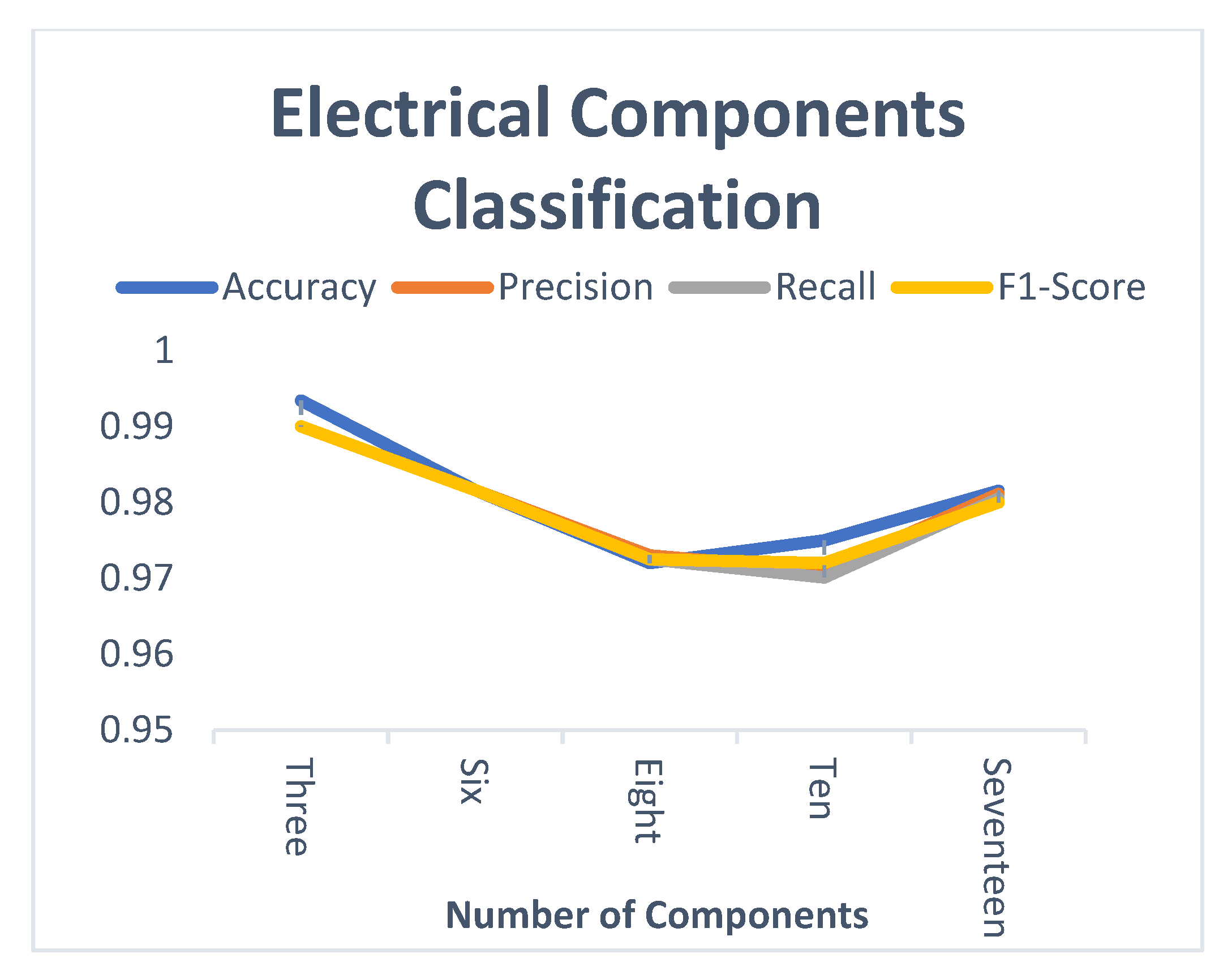
- The proposed model experimented extensively with different numbers of components, and it outperforms the existing state-of-the-art with higher attained accuracy and precision.
2. Related Work
2.1. Mechanical Components Classification
2.2. Electrical Components Classification
2.3. Feature Fusion
3. Materials and Methods
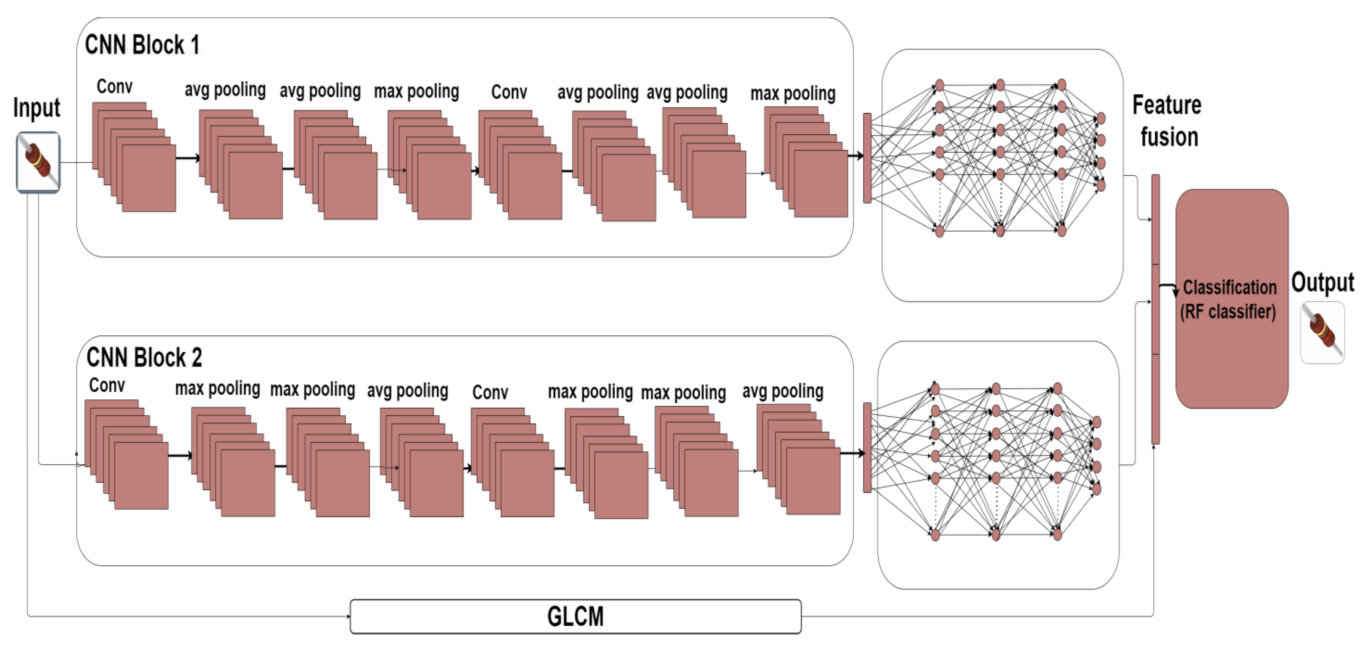
3.1. IMCCM Design
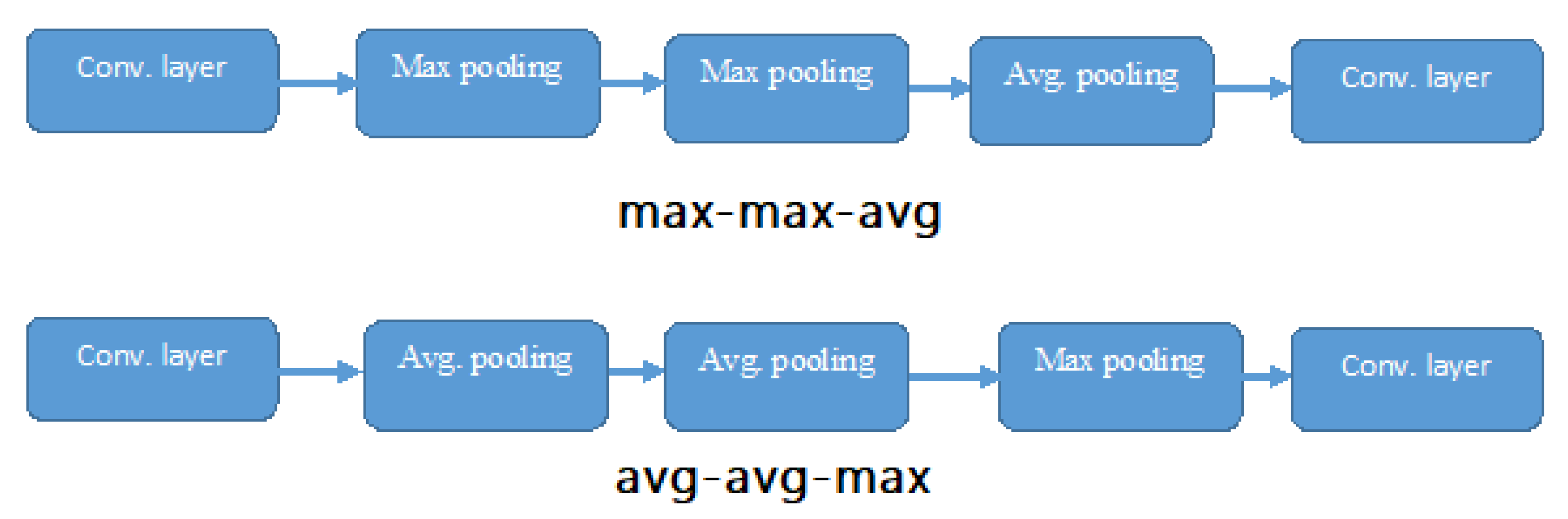
3.2. D-S Pooling Layer
3.3. Hyperparameter Tuning, Loss Function, and Optimization
3.4. Grey-Level-Co-Variance-Matrix (GLCM)
3.4.1. Correlation
3.4.2. Contrast
3.4.3. Dissimilarity
3.5. Feature Fusion
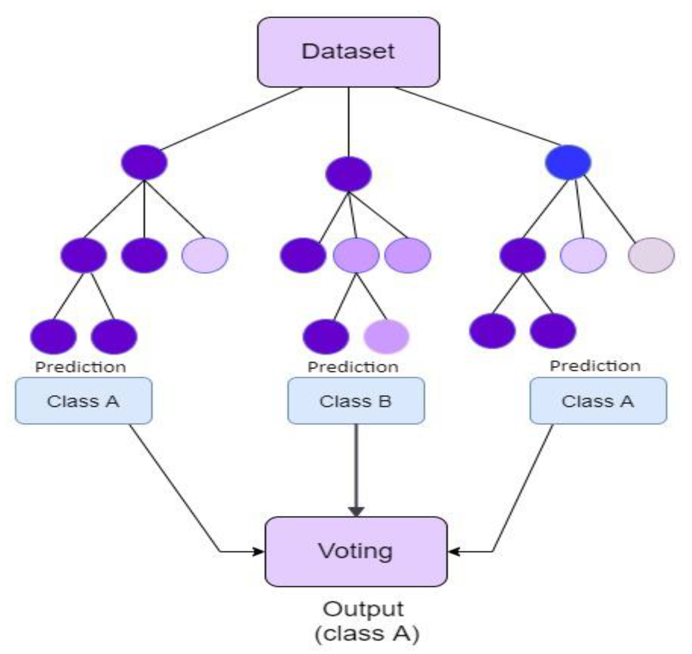
3.6. Random Forest Classifier
4. Experiment Results and Analysis
4.1. Dataset
4.2. Data pre-Processing and Augmentation
4.3. Performance Evaluation
4.4. Experiment Results
4.5. Discussion
5. Conclusions
Author Contributions
Funding
Data Availability Statement
Conflicts of Interest
References
- Canziani, A.; Culurciello, E.; Paszke, A. Evaluation of neural network architectures for embedded systems. In Proceedings of the 2017 IEEE International Symposium on Circuits and Systems (ISCAS), Baltimore, MD, USA, 28–31 May 2017; pp. 1–4. [Google Scholar]
- Krizhevsky, A.; Sutskever, I.; Hinton, G.E. Imagenet classification with deep convolutional neural networks. In Proceedings of the Advances in Neural Information Processing Systems, Lake Tahoe, NV, USA, 3–6 December 2012; pp. 1097–1105. [Google Scholar]
- Liu, Z.; Zhao, B.; Zhu, H. Research of Sorting Technology Based on Industrial Robot of Machine Vision. In Proceedings of the 2012 Fifth International Symposium on Computational Intelligence and Design, Hangzhou, China, 28–29 October 2012; pp. 57–61. [Google Scholar] [CrossRef]
- Fechteler, M.; Schlüter, M.; Krüger, J. Prototype for enhanced product data acquisition based on inherent features in logistics. In Proceedings of the 2016 IEEE 21st International Conference on Emerging Technologies and Factory Automation (ETFA), Berlin, Germany, 6–9 September 2016; pp. 1–4. [Google Scholar]
- Rawat, W.; Wang, Z. Deep Convolutional Neural Networks for Image Classification: A Comprehensive Review. Neural Comput. 2017, 29, 2352–2449. [Google Scholar] [CrossRef] [PubMed]
- Yu, D.; Wang, H.; Chen, P.; Wei, Z. Mixed pooling for convolutional neural networks. In Rough Sets and Knowledge Technology: 9th International Conference, RSKT 2014, Shanghai, China, 24–26 October 2014; Springer International Publishing: Berlin/Heidelberg, Germany, 2014; pp. 364–375. [Google Scholar]
- Schlüter, M.; Niebuhr, C.; Lehr, J.; Krüger, J. Vision-based identification service for remanufacturing sorting. Procedia Manuf. 2018, 21, 384–391. [Google Scholar] [CrossRef]
- You, F.C.; Zhang, Y.B. A Mechanical Part Sorting System Based on Computer Vision. In Proceedings of the 2008 International Conference on Computer Science and Software Engineering, Washington, DC, USA, 12–14 December 2008. [Google Scholar]
- Wang, Y.F.; Chen, H.D.; Zhao, K.; Zhao, P. A Mechanical Part Sorting Method Based on Fast Template Matching. In Proceedings of the 2018 IEEE International Conference on Mechatronics, Robotics, and Automation (ICMRA), Hefei, China, 18–21 May 2018; pp. 135–140. [Google Scholar] [CrossRef]
- Cicirello, V.; Regli, W. An approach to a feature-based comparison of solid models of machined parts. AI EDAM 2002, 16, 385–399. [Google Scholar] [CrossRef]
- Wei, B.; Hu, L.; Zhang, Y.; Zhang, Y. Parts Classification based on PSO-BP. In Proceedings of the 2020 IEEE 4th Information Technology, Networking, Electronic and Automation Control Conference (IT-NEC), Chongqing, China, 12–14 June 2020; pp. 1113–1117. [Google Scholar] [CrossRef]
- Dong, Q.; Wu, A.; Dong, N.; Feng, W.; Wu, S. A convolution neural network for parts recognition using data augmentation. In Proceedings of the 2018 13th World Congress on Intelligent Control and Automation (WCICA), Changsha, China, 4–8 July 2018; pp. 773–777. [Google Scholar]
- Yildiz, E.; Wörgötter, F. DCNN-based screw classification in automated disassembly processes. In Proceedings of the International Conference on Robotics, Computer Vision and Intelligent Systems (ROBOVIS 2020), Budapest, Hungary, 4–6 November 2020; pp. 61–68. [Google Scholar]
- Taheritanjani, S.; Haladjian, J.; Bruegge, B. Fine-grained visual categorization of fasteners in overhaul processes. In Proceedings of the 2019 5th International Conference on Control, Automation and Robotics (ICCAR), Beijing, China, 19–22 April 2019; pp. 241–248. [Google Scholar]
- Hossain, M.E.; Islam, A.; Islam, M.S. A proficient model to classify Bangladeshi bank notes for automatic vending machine Using a tıny dataset with One-Shot Learning & Siamese Networks. In Proceedings of the 2020 11th International Conference on Computing, Communication and Networking Technologies (ICCCNT), Kharagpur, India, 1–3 July 2020; pp. 1–4. [Google Scholar]
- Tastimu, C.; Akin, E. Fastener Classification Using One-shot learning with siamese convolution networks. JUCS—J. Univers. Comput. Sci. 2022, 28, 80–97. [Google Scholar] [CrossRef]
- Wang, B. Base and current situation of data standardization for electronic components & devices. Electron. Compon. Device Appl. 2010, 11, 30–32. [Google Scholar]
- Du, S.S.; Shan, Z.D.; Huang, Z.C.; Liu, H.Q.; Liu, S.L. The algorithmic of components auto-classification and system development of electronic components. Dev. Innov. Mach. Electr. Prod. 2008, 6, 133–135. [Google Scholar]
- Moetesum, M.; Younus, S.W.; Warsi, M.A.; Siddiqi, I. Segmentation and recognition of electronic components in hand-drawn circuit diagrams. ICST Trans. Scalable Inf. Syst. 2018, 5, 154478. [Google Scholar] [CrossRef]
- Salvador, R.; Bandala, A.; Javel, I.; Bedruz, R.A.; Dadios, E.; Vicerra, R. DeepTronic: An electronic device classification model using deep convolutional neural networks. In Proceedings of the 2018 IEEE 10th International Conference on Humanoid, Nanotechnology, Information Technology, Communication, and Control, Environment, and Management (HNICEM), Baguio City, Philippines, 29 November–2 December 2018; pp. 1–5. [Google Scholar] [CrossRef]
- Wang, Y.J.; Chen, Y.T.; Jiang, Y.S.F.; Horng, M.F.; Shieh, C.S.; Wang, H.Y.; Ho, J.H.; Cheng, Y.M. An artificial neural network to support package classification for SMT components. In Proceedings of the 2018 3rd International Conference on Computer and Communication Systems (ICCCS), Nagoya, Japan, 27–30 April 2018; pp. 130–134. [Google Scholar] [CrossRef]
- Atik, I. Classification of electronic components based on convolutional neural network Architecture. Energies 2022, 15, 2347. [Google Scholar] [CrossRef]
- Kaya, V.; Akgül, I. Classification of electronic circuit elements by machine learning based methods. In Proceedings of the 6th International Conference On Advances In Proceedings of the Natural & Applied Science Engineering, Online, 11–13 October 2022. [Google Scholar]
- Hu, S.; Zhang, X.; Liao, H.Y.; Liang, X.; Zheng, M.; Behdad, S. Deep learning and machine learning techniques to classify electrical and electronic equipment. In Proceedings of the ASME International Design Engineering Technical Conferences & Computers and Information in Engineering Conference, IDETC/CIE 2021, Online, 17–20 August 2021. [Google Scholar]
- Lefkaditis, D.; Tsirigotis, G. Morphological feature selection, and neural classification. J. Eng. Sci. Technol. Rev. 2009, 2, 151–156. [Google Scholar] [CrossRef]
- Hu, X.; Xu, J.; Wu, J. A novel electronic component classification algorithm based on hierarchical convolution neural network. In Proceedings of the IOP Conference Series: Earth and Environmental Science, Changchun, China, 21–23 August 2020; Volume 474, p. 052081. [Google Scholar] [CrossRef]
- Cheng, Y.; Wang, A.; Wu, L. A Classification Method for electronic components based on Siamese network. Sensors 2022, 22, 6478. [Google Scholar] [CrossRef] [PubMed]
- Ali, F.; Sappagh, S.A.; Islam, S.M.R.; Kwak, D.; Ali, A.; Imran, M.; Kwak, K.S. A smart healthcare monitoring system for heart disease prediction based on ensemble deep learning and feature fusio. Inf. Fusion 2020, 63, 208–222, ISSN 1566-2535. [Google Scholar] [CrossRef]
- Yang, L.; Xie, X.; Li, P.; Zhang, D.; Zhang, L. Part-based convolutional neural network for visual recognition. In Proceedings of the 2017 IEEE International Conference on Image Processing, Beijing, China, 17–20 September 2017; pp. 1772–1776. [Google Scholar]
- Cai, H.; Qu, Z.; Li, Z.; Zhang, Z.; Hu, X.; Hu, B. Feature-level fusion approaches based on multimodal EEG data for depression recognition. Inf. Fusion 2020, 59, 127–138. [Google Scholar] [CrossRef]
- Kang, Z.; Yang, J.; Li, G.; Zhang, Z. An automatic garbage classification system based on deep learning. IEEE Access 2020, 8, 140019–140029. [Google Scholar] [CrossRef]
- Fradi, H.; Fradi, A.; Dugelay, J. Multi-layer Feature Fusion and selection from convolutional neural networks for texture classification. In Proceedings of the 16th International Joint Conference on Computer Vision, Imaging and Computer Graphics Theory and Applications, Vienna, Austria, 8–10 February 2021; Volume 4, pp. 574–581, ISSN 2184-4321. [Google Scholar]
- Caglayan, A.; Buak, C.A. Exploiting multilayer features using a CNN-RNN approach for RGB-D object recognition. In Proceedings of the European Conference on Computer Vision (ECCV) Workshops, Munich, Germany, 8–14 September 2018. [Google Scholar]
- Pan, Y.; Zhang, L.; Wu, X.; Skibniewski, M.J. Multi-classifier information fusion in risk analysis. Inf. Fusion 2020, 60, 121–136. [Google Scholar] [CrossRef]
- Agarap, A.F. Deep Learning Using Rectified Linear Units (Relu). arXiv 2008, arXiv:1803.08375. [Google Scholar]
- Kingma, D.; Ba, J. Adam: A method for stochastic optimization. arXiv 2014, arXiv:1412.6980,. [Google Scholar]
- Bo, H.; Ma, F.L.; Jiao, L.C. Research on computation of GLCM of image texture. Acelectronicaica Sin. 2006, 34, 155. [Google Scholar]
- Pal, M. Random forest classifier for remote sensing classification. Int. J. Remote Sens. 2005, 26, 217–222. [Google Scholar] [CrossRef]
- Huang, G.; Liu, Z.; Maaten, V.D.; Weinberger, K.Q. Densely connected convolutional networks. In Proceedings of the IEEE conference on computer vision and pattern recognition, Honolulu, HI, USA, 21–26 July 2017; pp. 4700–4708. [Google Scholar]
- Simonyan, K.; Zisserman, A. Very deep convolutional networks for large-scale image recognition. arXiv 2014, arXiv:1409.1556. [Google Scholar]
- He, K.; Zhang, X.; Ren, S.; Sun, J. Deep residual learning for image recognition. In Proceedings of the IEEE conference on computer vision and pattern recognition, Las Vegas, NV, USA, 27–30 June 2016; pp. 770–778. [Google Scholar]
- Chollet, F. Xception: Deep learning with depthwise separable convolutions. In Proceedings of the IEEE conference on computer vision and pattern recognition, Honolulu, HI, USA, 21–26 July 2017; pp. 1251–1258. [Google Scholar]


| Authors | No. of Components | Techniques | Type of Components | Datasets Size | Training Accuracy (%) | Testing Accuracy (%) |
|---|---|---|---|---|---|---|
| Dong et al. (2018) [12] | AlexNet | Screw, Nut, Washer | 40 | - | 95.4 | |
| Yildiz (2020) [13] | 12 | EfficientNet, DenseNet, ResNet | Screws | 20,000 | 96.1 | 97 |
| Taheritanjani et al. (2019) [14] | 2 | AlexNet, VGG16, Inception v3 | Bolt, Washer | 1300 | 100 | 99.4 |
| Slavander et al. (2018) [20] | 6 | Inception-v3, GoogleNet, and Resnet101 | Resistors, inductor, Capacitor, Transistor, Diode, Transformer, IC | 632 | 100 | 94.64 |
| Atik (2022) [22] | 3 | CNN | Capacitor, Diode, Resistor | 2708 | - | 98.99 |
| Kaya et al. (2022) [23] | 3 | SVM, RF, NB | Capacitor, Diode, Resistor | 2708 | 95.24 | |
| Hu et al. (2021) [24] | 3 | Naïve Bayes(Bernoulli, Gaussian, Multinomial distributions),SVM(Linear, Radial Basis Function (RBF)), VGG-16, GoogleNet, Inception-v3, Inception-v4 | Laptop HP, ThinkPad, Apple | 210 | 98.3 | 92.9 |
| Lefkaditis et al. (2009) [25] | 6 | Support Vector Machine(SVMs), Multilayeperceptron’s (MLPs) | Electrolytic Capacitors, Ceramic Capacitors, Resistor, Transistors, Power transistors | 87 | 92.3 | |
| Hu et al. (2020) [26] | 8 | Convolutional Automatic Coding | IC, Capacitor, Resistor, Inductance, Diode, LED, Speaker, Transistor | 4500 | - | 94.26 |
| Cheng et al. (2022) [27] | 17 | Siamese Network | - | 3094 | - | 94.6 |
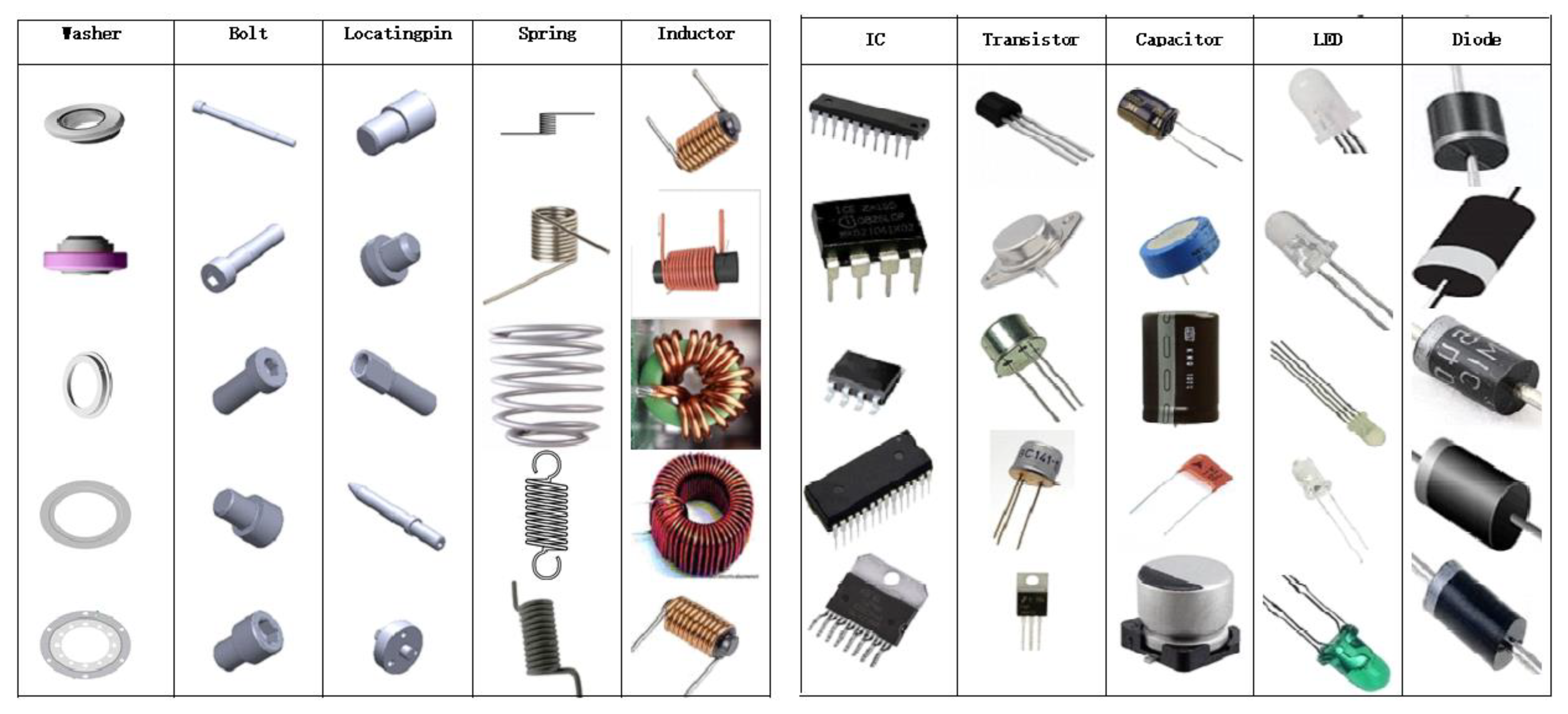
| Electrical Components | Size | Mechanical Components | Size |
|---|---|---|---|
| Resistor | 5104 | Nut | 1908 |
| Capacitor | 3719 | Plug | 1764 |
| Inductor | 1476 | Washer | 1908 |
| LED | 2004 | Spring | 2074 |
| IC | 2506 | Locating pin | 1908 |
| Transistor | 4504 | Bearing | 2230 |
| Transformer | 2639 | Bolt | 1908 |
| Diode | 3391 | ||
| Push button | 2508 | ||
| Potentiometer | 2694 | ||
| Total | 30,545 | Total | 13,700 |
| Model | Training Accuracy | Validation Accuracy | No. of Trainable Parameters | |
|---|---|---|---|---|
| Densenet201 | 97.3 | 94.9 | 18,216,977 | |
| Densenet121 | 98.9 | 93.5 | 7,020,561 | |
| EfficientNetB1 | 98.56 | 91.6 | 6,596,273 | |
| Resnet50 | 97.03 | 69.8 | 23,666,833 | |
| VGG16 | 84.4 | 86.5 | 15,010,769 | |
| VGG19 | 83.9 | 84.8 | 20,320,465 | |
| InceptionV3 | 94.4 | 95.6 | 21,900,593 | |
| Xception | 98.8 | 97.5 | 21,987,769 | |
| Our Model | Block 1 | 92.02 | 90.45 | 60,433 |
| Block 2 | 92.47 | 91.39 | 80,913 | |
| IMCCM | 98.15 | 141,346 | ||
| Datasets | CNN | Top-1 Accuracy | Top-5 Accuracy | No. of Trainable Parameters | Image Size |
|---|---|---|---|---|---|
| CIFAR-10 | Block 1 | 67.98 | 97.26 | 47,690 | 32 × 32 |
| Block 2 | 71.4 | 98 | 47,690 | ||
| MNIST | Block 1 | 98.25 | 99.98 | 46,538 | 28 × 28 |
| Block 2 | 97.76 | 99.97 | 54,794 | ||
| Machine Components | Block 1 | 92.02 | 99.72 | 60,433 | 100 × 100 |
| Block 2 | 92.47 | 99.64 | 80,913 |
Disclaimer/Publisher’s Note: The statements, opinions and data contained in all publications are solely those of the individual author(s) and contributor(s) and not of MDPI and/or the editor(s). MDPI and/or the editor(s) disclaim responsibility for any injury to people or property resulting from any ideas, methods, instructions or products referred to in the content. |
© 2023 by the authors. Licensee MDPI, Basel, Switzerland. This article is an open access article distributed under the terms and conditions of the Creative Commons Attribution (CC BY) license (https://creativecommons.org/licenses/by/4.0/).
Share and Cite
Batool, A.; Dai, Y.; Ma, H.; Yin, S. Industrial Machinery Components Classification: A Case of D-S Pooling. Symmetry 2023, 15, 935. https://doi.org/10.3390/sym15040935
Batool A, Dai Y, Ma H, Yin S. Industrial Machinery Components Classification: A Case of D-S Pooling. Symmetry. 2023; 15(4):935. https://doi.org/10.3390/sym15040935
Chicago/Turabian StyleBatool, Amina, Yaping Dai, Hongbin Ma, and Sijie Yin. 2023. "Industrial Machinery Components Classification: A Case of D-S Pooling" Symmetry 15, no. 4: 935. https://doi.org/10.3390/sym15040935