Special Functions and Its Application in Solving Two Dimensional Hyperbolic Partial Differential Equation of Telegraph Type

Abstract

In this article, we use the applications of special functions in the form of Chebyshev polynomials to find the approximate solution of hyperbolic partial differential equations (PDEs) arising in the mathematical modeling of transmission line subject to appropriate symmetric Dirichlet and Neumann boundary conditions. The special part of the model equation is discretized using a Chebyshev differentiation matrix, which is centro-asymmetric using the symmetric collocation points as grid points, while the time derivative is discretized using the standard central finite difference scheme. One of the disadvantages of the Chebyshev differentiation matrix is that the resultant matrix, which is obtained after replacing the special coordinates with the derivative of Chebyshev polynomials, is dense and, therefore, needs more computational time to evaluate the resultant algebraic equation. To overcome this difficulty, an algorithm consisting of fast Fourier transformation is used. The main advantage of this transformation is that it significantly reduces the computational cost needed for N collocation points. It is shown that the proposed scheme converges exponentially, provided the data are smooth in the given equations. A number of numerical experiments are performed for different time steps and compared with the analytical solution, which further validates the accuracy of our proposed scheme.

1. Introduction

Special functions play a key role in solving and providing the inside details in theories of differential equations. They are most commonly used to solve partial and ordinary differential equations (ODEs). In recent years, the application of these functions has been extended for the solution of fractional, integro-differential and stochastic differential equations arising during the mathematical modeling of many real word problems in science and engineering. These special functions especially arise while solving partial differential equations; when it is reduced, the set of equations consists of ODEs by the separation of variables with partial derivatives. The most common special functions are Gamma, Zeta, Bessel, Legendre, Laguerre, Hermite, Chebyshev polynomials, hypergeometric and many more functions. Orthogonal polynomials and their sophisticated properties are considered to be the backbone of the solution of differential equations. They are used to solve these differential equations more accurately and with high precision of accuracy. Their orthogonal properties are used with respect to some weight functions and are used for some choices of parameters involved in these differential equations to investigate their accuracy and stability region, especially in the investigation of approximate solutions for PDEs, which are time-dependent [1]. Many numerical methods for the approximate solution of differential equations use polynomials as an approximation to the unknown function. One such method that uses orthogonal polynomials as a basis function is known as a spectral method.

Spectral methods use the global approach during the approximation of any unknown function. In this approach, the computation depends at any point on the entire domain in addition to the neighboring points opposite the local approaches, where the computation only depends on the neighboring points. These methods are mostly used for the discretization of special coordinates. Their formulation mainly depends on the approximation and test functions, also called the trail and weight functions, respectively. The linear combination of these trail functions is used as an approximating function to get the approximate solution of differential equations. To ensure that the differential equations are subject to appropriate conditions, either initial or boundaries, are satisfied, the test function’s truncated series expansion is used. A suitable norm is used to achieve this by minimizing the error instead of the exact solution using the solution of truncated series and receiving the implicit or explicit residual counts. This is one of the reasons that spectral methods were treated as a special case of the method of residuals, which is equivalent to a suitable orthogonality condition being satisfied by the residual subject to some test functions. The feature that distinguishes the early version of the spectral method from its finite element and finite difference counterpart is the choice of a trial function. The earliest three types of spectral methods that distinguish them from each other is the choice of the test function, that is Galerkin, Tau and collocation methods. For the periodic function, Fourier spectral methods are used for discrete data, while for the non-periodic domain, the theory of orthogonal polynomials, such as Legendre or Chebyshev polynomials, basis functions are the best choice [2,3]. In this research work, we will use the applications of Chebyshev polynomials together with the FFT to solve the hyperbolic PDEs of telegraph type. High-order methods and their analysis based on the polynomial approximation and their properties are studied in detail [4,5,6,7,8,9,10,11,12,13].

Oliver Heaviside was the first person who worked on telegraph equations and studied, in detail, the second-order hyperbolic PDEs that arise from the mathematical modeling of the voltage and current on an electrical transmission line with distance. This model explains that the wave sequence that can form with the line and the electromagnetic waves can be reflected on the wire. Recently, it has been discovered that the telegraph equation is the best candidate as an alternative to the diffusion equation while investigating turbulence transport in its early phase. This is because, in early times, the movement of the particles was ballistic, and they scattered with the passage of time. The coefficient of diffusion during the running time, was determined numerically for example, for instance, by tracing the mean square displacement of ensemble particles. The reflection of this behavior is increasing linearly with respect to ballistic motion. The other problem is that the speed of the particles is finitely propagated, which is also considered as there is no magnetostatic turbulence at all or is very limited. Due to the fixed energy of the particles, it cannot have a finite probability of filling the space when the source is at a large distance. In contrast, the telegraph equation has great potential to differentiate between the early ballistic motion of particles and the diffusive transport at a later stage. This is due to the fact that the telegraph equation consists of an additional scale of time, which produces behavior like a wave. For this reason, the telegraph equation is used for the mathematical description of pulse propagation along a wire. At the beginning, at least, this behavior looks to have a very good agreement with the propagation of particle speed charged by the available energy [14]. The telegraph equation is most commonly used for the transmission of electrical signals and their propagation in signal analysis. In biological sciences, the telegraph equation can be used for the linearization of neurons of nerves and in muscle cells, the telegraph equations lead to how the pressure waves of pulsating blood flow in the arteries are reproduced. The movement of an insect through a fence in one dimension can also be studied by the telegraphic equation [15].

Unlike the other PDEs, such as parabolic and elliptic, the hyperbolic PDEs are considered to be more useful in many research fields of science and technology, especially in the field of applied sciences, where these equations are used to understand the most important features of some real-world problems. A numerical algorithm is used to solve the hyperbolic PDEs of telegraph type in [16,17]. There are numerous areas in which telegraph equations are being used, and most of them are related to the field of engineering and sciences. For example, the structure of vibrations, signal analysis in a cable of transmission line, wave propagation and the theory of random walk [18,19,20]. To solve the hyperbolic PDEs based on telegraph equation, analysis is usually difficult, and, therefore, numerical methods are the alternate choices. The most common numerical schemes to solve hyperbolic PDEs are based on the classical finite difference, finite elements and spectral schemes, where the first two use the local approach while the latter one uses the global approach, which makes it superior compared to other ones. In the past few years, many mathematicians have worked on the development of numerical schemes to solve the hyperbolic equation of order two along the constant coefficients. Some scientists have applied the finite element method for solving non-homogeneous telegraph equations. For short compact support, the multi-wavelet bases that were explained by Albert are infinitely differentiable. That means one can use these bases for both finite difference and spectral methods. Albert multi-wavelet are the bases that can be used to find the solution to the nonlinear time-dependent partial differential equations [21]. Some other multi-wavelet methods have been introduced in [22,23,24].

Various other numerical methods have been used to solve the hyperbolic PDEs; for example, a mesh-less method using the radial basis function has been used to solve the Klein–Gordon equation in [25]. The method of finite difference for the approximate solution of nonlinear obstacles has been used in the two-dimension equation by Ling et al. [26], while Abbas et al. proposed a numerical scheme using the shifted form of Chebyshev polynomials and its operational matrices derived from its derivative and integrals [27]. A numerical approach based on dual reciprocity boundary integral equations (DRBI) was used in [28], while differential quadrature methods for the proposed model in two dimensions with appropriate boundary and initial conditions were investigated and derived in [29]. The telegraph equations in two-dimensional initial value problems consisting of hyperbolic PDEs were solved by the local Petrov Galerkin method [30]. An alternating direction for implicit schemes consisting of a compact difference scheme of order four for telegraph equations is used in [31], the mesh-less hybrid method [32] and by mesh-less collocation method [33]. These equations in early work were solved by the non-polynomial spline method [34], the discrete eigenfunctions method [35], the differential transform method [36], Adomian method [37] and the kernel method, which was used to solve the nonlinear telegraph equations [38], which depends upon the Rothe’s approximation method. The generalized finite difference scheme is applied in [39], while the multi-wavelet Galerkin method is discussed by [40].

The telegraph equation of fractional order using the analytical approach based on the Shehu transform was investigated in [41], where the technique was applied to one, two and three-dimensional equations. A method based on the decomposition method for a multi-dimensional equation of telegraph type with a fractional order using Elzaki transform has been studied in [42]. A numerical scheme using radial function as a basis combined with collocation points for the approximate solution for the hyperbolic equation in one dimension is used by the authors in [43]. The idea of this technique is similar to a finite difference scheme. Berna et al. introduced an efficient numerical approximation technique using Taylor’s polynomial approach to solve the constant coefficients of hyperbolic PDEs [44]. This technique was the improved version of Taylor’s matrix scheme, which is commonly used for solving ordinary, integral and differential equations. A stable and accurate finite difference scheme of level three in the compact form of order four is examined in detail for a second-order, two-dimensional hyperbolic equation in [45]. In recent years, some numerical techniques that are based on the Bernoulli Collocation method and Chebyshev collocation in combination with the Runge–Kutta method were investigated in [46,47], unlike our proposed scheme, which is also based on Chebyshev polynomials in conjunction with FFTs in special coordinates, the second-order finite difference scheme was in temporal one. Recently, these methods have been successfully applied while investigating some real word problems [48,49,50,51,52,53]. For more applications of special functions, we refer the reader to [54,55,56].

The main purpose of the current paper is to construct an efficient numerical scheme for solving two-dimensional hyperbolic PDEs based on the telegraph equation with appropriate boundary conditions. For this reason, a spectral collocation method based on a Chebyshev polynomial in conjunction with fast Fourier transform (FFT) is used in special coordinates, while the temporal part is evaluated using a second-order finite difference scheme. The almost antisymmetric Chebyshev differentiation matrix, which results from discretizing the special part, is evaluated using the symmetric collocation points based on Gauss–Lobatto points, which are the roots of Chebyshev polynomials with the help of FFT. Our motivation is further enhanced by the high precision and low phase error of spectral methods for solving the proposed problem. The main advantage of spectral methods is that the error decay is exponential; that is, the convergence rate is infinite in space for a very small number of collocations points. They are very flexible in terms of choosing a basis function. One can choose any basis function depending on the problem. The disadvantage is that they are hard to implement, and they use global functions as a basis function. For this reason, they are not well suited to handle the local features as well as Sharp gradients, for example, the Gibbs phenomenon.

The remaining structure of the paper includes the method and mathematical formulations in Section 2. Some preliminaries needed for the analysis of the proposed scheme are introduced in Section 3. Numerical simulations for different time steps to confirm the exponential convergence are obtained in Section 4, while a conclusion is drawn in Section 5.

2. Mathematical Model and Method Description

In general second-order PDEs of parabolic, elliptic or hyperbolic types, linear or nonlinear plays an essential role in many applications in science and engineering. The telegraph PDEs which is formulated from a line of telegraph is used for a signal as transmission medium is one of these applications. Due to the hyperbolic nature of telegraph PDEs, unlike elliptic and parabolic PDEs, there is no inherited physical dissipation in hyperbolic PDEs. This means that a very small error for any resolved phenomena under consideration can cause any numerical scheme to be unstable. This stability issue is more severe in spectral techniques compared to any other technique used for the approximate solutions of these hyperbolic PDEs. This is one of the reasons that it does not accept the higher-order methods, particularly the spectral collocation method for the Gibbs phenomenon appearing in the solution, which causes discontinuity in the solution during a finite time interval. If the stability is, however, maintained for a sufficiently long time step, it appears only to be first-order, which makes the use of high-order methods questionable. All these issues are very genuine, and careful attention is needed for them. However, if spectral collocation methods are applied correctly, they are not causing any problems.

The generalized telegraph equation is a non-homogeneous telegraph along the boundary, and the initial conditions are demonstrated as

$$v_{tt}(x,y,t)+2\xi v_t(x,y,t)+{\eta }^{2}v(x,y,t)=v_{xx}(x,y,t)+v_{yy}(x,y,t)+g(x,y,t),$$

(1)

where $\xi$ and $\eta$ are constants that are real along with initial and Dirichlet boundary conditions. Equation (1) becomes the damped wave motion when $\xi >0$ and $\eta$ = 0.

$$v(x,y,0)=g_0(x,y),\frac{\partial v}{\partial t}(x,y,0)=g_1(x,y),$$

(2)

$$v(-1,y,t)=f_0(y,t),v(1,y,t)=f_1(y,t),v(x,-1,t)=f_2(x,t),v(x,1,t)=f_3(x,t)$$

(3)

Chebyshev spectral differentiation via FFT (Fast Fourier transform) is used to approximate the spatial domain in the x and y-directions, and the Finite difference scheme of order two approximates the time domain. For a unit circle $\left|z\right|=1$, suppose z is a complex number. Suppose $\varphi$ is the argument of z that can be found up to the multiples of $2\pi$. Suppose $x=Real\left(z\right)=cos\left(\varphi \right)$ for every $x\in [-1,1]$, and their two complex conjugates are

$$x=Real\left(z\right)=\frac{1}{2}(z+z^{-1})=cos\left(\varphi \right)\in [-1,1]$$

(4)

The $mth$ Chebyshev polynomial is represented by $T_m$. Then, generally, $T_{m+1}$ can be defined by

$$T_{m+1}\left(x\right)=\frac{1}{2}(z^{m+1}-z^{-m-1})=\frac{1}{2}(z^m+z^{-m})(z+z^{-1})-\frac{1}{2}(z^{m-1}+z^{1-m})$$

(5)

For recurrence relation

$$T_{m+1}\left(x\right)=2x{T}_m\left(x\right)-T_{m-1}\left(x\right)$$

(6)

First, the derivatives in the x-direction, with the help of the spectral method, are iterated by taking the points $u_0,u_1,u_2,\dots ,u_M$ at Chebyshev points $x_0=1\dots x_{M-1}$ and expanding these data to the vector Y of length $2N$ with

$$Y_{2M-j}=u_j$$

(7)

where $j=1,2,\dots ,M-1$.

Now we are using fast Fourier transform to solve the equation.

$$Y_k=\frac{\pi }{N}\sum _{i=1}^{2M}ex{p}^{-\iota k{\varphi }_j}{Y}_j,$$

(8)

$k=-M+1,\dots ,M.$

At this point, we could define a new assumption as.

$$S=\iota k{u}_k,$$

(9)

rather than $Y_N=0.$ Now by using FFT to calculate the derivative of trigonometric interpolant P on an equispaced grid.

$$S_j=\frac{1}{2\pi }\sum _{k=-M+1}^{M}ex{p}^{\iota k{\varphi }_j}{S}_k,$$

(10)

where $j=1,2,\dots ,M.$ Now for algebraic polynomial interpolant p, compute the derivative on interior grid points by

$$s_j=-\frac{Z_j}{\sqrt{1-x_j^2}}.$$

(11)

where $j=1,\dots ,M-1,$ with special endpoint formulas:

$$s_j=\frac{1}{2\pi }{\sum _{m=0}^M}^{}{m}^2{u}_m,$$

(12)

$$s_M=\frac{1}{2\pi }{\sum _{m=0}^M}^{}{(-1)}^{m+1}{m}^2{u}_m,$$

(13)

and the terms $m=0,\dots ,M$ are multiplied by $\frac{1}{2}$. We can explain the above formulas by solving discrete inverse Fourier transform at $\varphi$.

$$Q\left(\varphi \right)=\frac{1}{2\pi }\sum _{k=-M+1}^{M}ex{p}^{ik\varphi }{u}_k=\sum _{m=0}^M{b}_{m}cosm\varphi ,$$

(14)

Now the algebraic polynomial interpolant of $u_j$ is $q\left(x\right)=Q\left(\varphi \right),$ where $x=cos\left(\varphi \right)$, now by calculating its derivative,

$$p^{\prime }\left(x\right)=\frac{P^{\prime }\left(\varphi \right)}{\frac{dx}{d\varphi }}=\frac{-{\sum }_{m=0}^{M}m{b}_{m}sinm\varphi }{-sin\varphi }=\frac{{\sum }_{m=0}^{M}m{b}_{m}sinm\varphi }{\sqrt{1-x^2}}.$$

(15)

To calculate the value of $p^{\prime }\left(x\right)$ at $x=\pm 1,$ we apply L’Hospital’s rule, which gives

$$p^{\prime }\left(1\right)=\sum _{m=0}^M{m}^2{b}_m,p^{\prime }{(-1)}^{m+1}{m}^2{b}_m,$$

(16)

Similarly, if the second derivative is required

$$p^{″}\left(x\right)=\frac{x{P}^{\prime }\varphi }{{(1-x^2)}^{\frac{3}{2}}}+\frac{P^{″}\left(\varphi \right)}{1-x^2},$$

(17)

If $S_j$ and $S_j^{\left(2\right)}$ are the first and second derivatives on an equispaced grid, then the second derivative of the Chebyshev grid is expressed as

$$s_j^{\left(2\right)}=\frac{-x{S}_j}{{(1-x_j^2)}^{\frac{3}{2}}}+\frac{S_j^{\left(2\right)}}{1-x_j^{\left(2\right)}},1\le j\le M-1$$

(18)

where $S_j$ and $S_j^{\left(2\right)}$ are the derivatives of the first and second orders on the equispace grid, respectively. For simplicity, let us suppose that ${\nu }_{xx}=s_j^{\left(2\right)}$. Now we have to solve the time derivative with finite difference method with a central difference.

$$\frac{\partial v}{\partial t}(x,t)=\frac{v^{i+1}-v^{i-1}}{2\Delta t},$$

(19)

and

$$\frac{{\partial }^{2}v}{{\partial }^{2}t}(x,t)=\frac{v^{i+1}-2v^j+v^{i-1}}{{(\Delta t)}^2},$$

(20)

Now we are solving the left-hand side of the general equation. We put the values on the left-hand side of the general equation

$$\frac{v^{i+1}-2v^i+v^{i-1}}{{(\Delta t)}^2}+2\eta \left(\frac{v^{i+1}-v^{i-1}}{2\Delta t}\right)+{\xi }^2{v}^i={\nu }_{xx}+{\nu }_{yy}+g,$$

(21)

$$\frac{v^{i+1}-2v^i+v^{i-1}}{{(\Delta t)}^2}+\left(\frac{\eta v^{i+1}-\eta v^{i-1}}{\Delta t}\right)+{\xi }^2{v}^i={\nu }_{xx}+{\nu }_{yy}+g,$$

(22)

$$\frac{v^{i+1}-2v^i+v^{i-1}+\eta \Delta t{v}^{i+1}-\eta \Delta t{v}^{i-1}+\Delta t^2{\xi }^2{v}^i}{\Delta t^2}={\nu }_{xx}+{\nu }_{yy}+g,$$

(23)

$$\frac{v^{i+1}(1+\eta \Delta t)+v^i(\Delta t^2{\xi }^2-2)+v^{i-1}(1-\eta \Delta t)}{\Delta t^2}={\nu }_{xx}+{\nu }_{yy}+g,$$

(24)

$$v^{i+1}=\frac{1}{1+\eta \Delta t}[\Delta t^2\left({\nu }_{xx}+{\nu }_{yy}\right)+\Delta t^{2}g-v^i(\Delta t^2{\xi }^2-2)-v^{i-1}(1-\eta \Delta t)],$$

(25)

by putting the value of ${\nu }_{xx},$ we receive the resulting equation as

$$\begin{array}{c}{v}^{i+1}=\frac{1}{1+\eta \Delta t}\left[\Delta t^2\left[\left(\frac{-x{S}_j}{{\left(1-x_j^2\right)}^{\frac{3}{2}}}+\frac{S_j^{\left(2\right)}}{1-x_j^2}\right)+\left(\left(\frac{-y{S}_j}{{\left(1-y_j^2\right)}^{\frac{3}{2}}}+\frac{S_j^{\left(2\right)}}{1-y_j^2}\right)\right]\right.\right.\\ +\Delta t^{2}g-v^i\left(\Delta t^2{\xi }^2-2\right)-v^{i-1}(1-\eta \Delta t).\end{array}$$

(26)

Fast Fourier Transformation

In this subsection, we will introduce the Fourier and fast Fourier transformation, in which the latter one we use together with the Chebyshev polynomials to speed up the simulations.

The use of Fourier transformation plays a key role in solving differential equations due to the fact that it converts the equation into a much easier one. Its resultant differential operator becomes the multiplicative operator and can be used for the derivative elimination of one independent variable. The use of inverse transformation recovers the original variable solution. To evaluate the discrete Fourier transform (DFT) and its inverse for a sequence, an algorithm called the fast Fourier transform is used. The main advantage of the FFT is that it converts the $O\left(N^2\right)$ calculations to $O\left(N\mathit{log}N\right)$ calculations, due to which a significant improvement can be seen while evaluating algebraic equations. The fast development algorithms for DFT date back to Carl Friedrich Gauss’s unpublished work in 1805, where he wanted it to interpolate the orbit of asteroids Pallas and Juno from pattern observations. Later on, in 1965, his method turned out to be very similar to the one used by James Cooley and John Tukey, who were credited commonly for their invention of the FFT set of rules of the modern day [57]. FFT is the most useful tool in any field of engineering sciences, especially in signal processing. The convolution of FFT uses the multiplication principle in the domain of frequency, which corresponds to the convolution in the time domain. DFT is used to transform the signal into an input in the frequency domain and then used for the inverse DFT to transform it back to the time domain. Since the days of Fourier, this technique has been known but was not pointed out by anyone. One of the reasons for this is that DFT takes a lot of time compared to the time taken for directly calculating the convolution. The definition of DFT is as follows

Let $y_0,y_1,y_2,\dots ,y_{M-1}$ be complex numbers, then the DFT is defined as

$$Y_k=\sum _{m=0}^{M-1}{y}_m{e}^{\frac{-2\iota \pi km}{M}},$$

(27)

where $k=0,1,\dots ,M-1$ and $e^{\frac{2\iota \pi }{M}}$ is elementary $mth$ root of 1.

3. Some Preliminaries and Error Analysis

In this section, before we state some results for the error analysis of the numerical scheme under consideration, we write some preliminary results, which are necessary for the theoretical analysis of the model equation and are used in numerical discretization as well. These results are based on the same theory as in [1,2,3].

The first kind of Chebyshev polynomial $T_m\left(x\right)$ is the solution to a singular S-L boundary value problem of the form

$$\frac{d}{dx}\left(\sqrt{1-x^2}\frac{d{T}_m\left(x\right)}{dx}\right)+\frac{m^2}{\sqrt{1-x^2}},$$

(28)

where $T_m\left(x\right)$ is bounded for all $x\in [-1,1]$.

The explicit form of Chebyshev polynomials is given by

$$T_m\left(x\right)=cos\left(narccosx\right).$$

(29)

Thus, $T_0\left(x\right)=1,T_1\left(x\right)=x,T_2\left(x\right)=2x^2-1,T_3\left(x\right)=4x^3-3x$, and so on…

The orthogonality condition of Chebyshev polynomials on $L_w^2\left(I\right),I:[-1,1]$ implies that:

$${\int }_{-1}^1{T}_m\left(x\right)T_n\left(x\right)=\frac{\pi }{2}{c}_m{\delta }_{nm},$$

(30)

where

$$c_m=\left\{\begin{array}{cc}2& n=0,\\ \\ 1& otherwise.\end{array}\right.$$

(31)

For any boundary value problem, the symmetric Chebyshev Gauss–Lobatto quadrature collocation points are:

$$x_k=-cos\frac{\pi }{M}k,$$

(32)

with

$$w_m=\left\{\begin{array}{cc}\frac{\pi }{2M}& k=0,M\\ \\ \frac{\pi }{M}& k\in [1,\dots ,M-1].\end{array}\right.$$

(33)

These are among the most popular collocation points for solving any boundary value problems, as it includes the end-points. It is, therefore, a clear advantage when one needs to impose boundary conditions.

The constant of normalization is given by:

$$\widehat{{\gamma }_m}=\left\{\begin{array}{cc}\frac{\pi }{2}& k\in [1,\dots ,M-1]\\ \\ \pi & k=0,M.\end{array}\right.$$

(34)

The resultant discrete expansion coefficients are then given by:

$$\widehat{u_m}=\frac{1}{\widehat{{\gamma }_m}}\sum _{k=0}^{M}u\left(x_k\right)T_m\left(x_k\right)w_k.$$

(35)

The relation given in Equation (30) is the roots of $(1-x^2)T_M^{\prime }\left(x\right)$, whose corresponding differentiation matrix entries are given by:

$$D_{ik}=\left\{\begin{array}{cc}\frac{-2M^2}{6}& i=k=0,\\ \\ \frac{\widehat{c_i}}{\widehat{c_k}}\frac{{(-1)}^{i+k+m}}{x_i-x_k}& i\ne k\\ \\ -\frac{x_i}{2(1-x_i^2)}& 0<i=k<M\\ \\ \frac{2M^2+1}{6}& i=k=M.\end{array}\right.$$

(36)

where $\widehat{c_0}=2=\widehat{c_M}$ and $\widehat{c_k}=1$, otherwise. One can easily see that this differentiation matrix is centro asymmetric as a result of the reflection symmetry of the nodal points. That is, $D_{ik}=-D_{M-i,M-k}$.

Lemma 1

([58]). Assume that $F_i\left(t\right)$ is the i-th Lagrange interpolation polynomial with the $(M+1)$-point Gauss Chebyshev, or Gauss–Radau Chebyshev, or Gauss–Lobatto Chebyshev points ${\left\{x_k\right\}}_{k=0}^M$. Then

$$\underset{t\in I}{max}\sum _{i=0}^N\left|F_i\left(t\right)\right|\le C\sqrt{N}.$$

Lemma 2.

Let $y\in H^m[-1,1]$ and denote $I_{N}y$, the polynomial interpolation polynomial with respect to $(M+1)$-Gauss type points ${\left\{x_k\right\}}_{k=0}^M$. Then

$${∥y-I_{M}y∥}_{L^2\left(I\right)}\le C{M}^{-m}{\left|y\right|}_{m,M}[-1,1],$$

$${∥y-I_{M}y∥}_{L^{\infty }\left(I\right)}\le C{M}^{3/4-m}{\left|y\right|}_{m,M}\left(I\right).$$

Using Lemmas 1 and 2, one can easily state and prove the following main results.

Theorem 1.

Assume that $u\left(x\right)\in H_w^p[-1,1]$ with $p>1/2$ and $0<p<q$, there exists a positive constant C, independent of M, such that

$$\parallel u-I_M{u\parallel }_{H_w^p[-1,1]}\le C{M}^{2p-q}{\left|u\right|}_{H_w^p[-1,1]}.$$

Similarly, if we consider the error estimate in $L_{\infty },$ in the discrete version of Chebyshev expansion, one loses a factor $M^{\frac{1}{2}}$ and achieves the following main results.

Theorem 2.

Assume that $u\left(x\right)\in H_w^p[-1,1]$ with $p>1/2$, there exists a positive constant C, independent of M, such that

$$\parallel u-I_M{u\parallel }_{H_w^p[-1,1]}\le C{M}^{\frac{1}{2}-p}{\left|u\right|}_{H_w^p[-1,1]}.$$

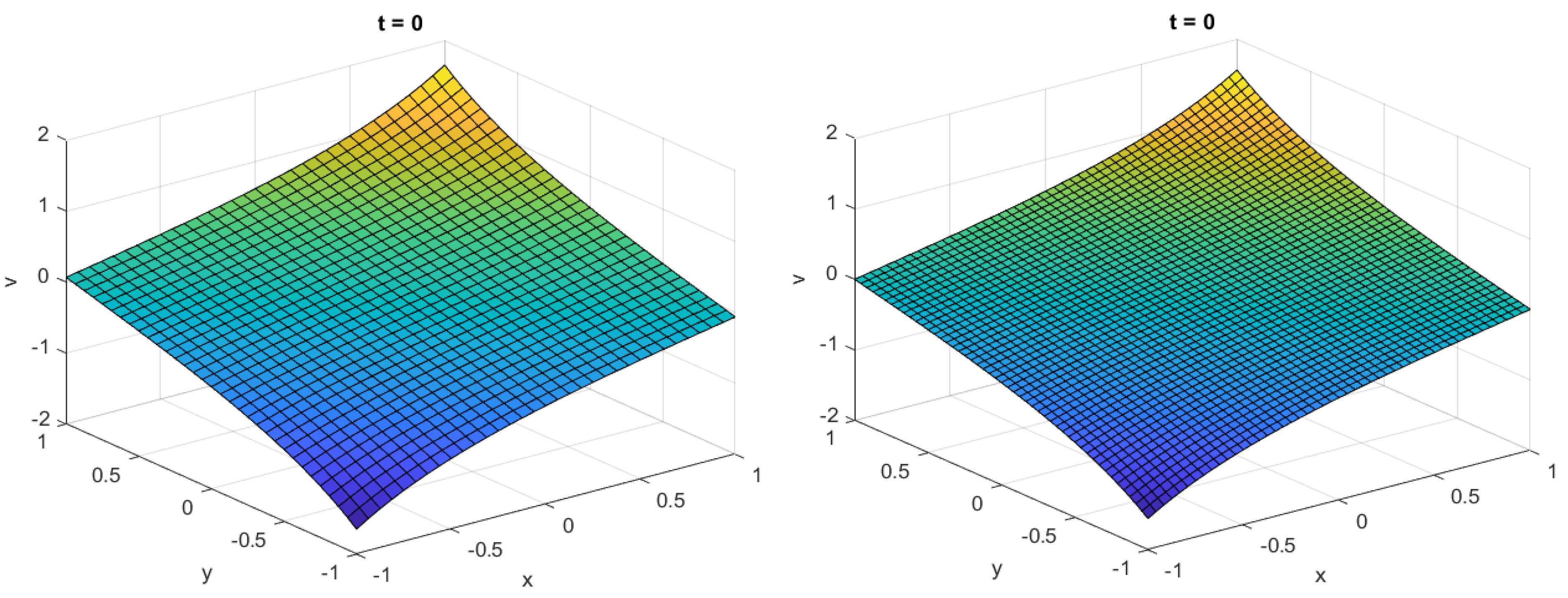
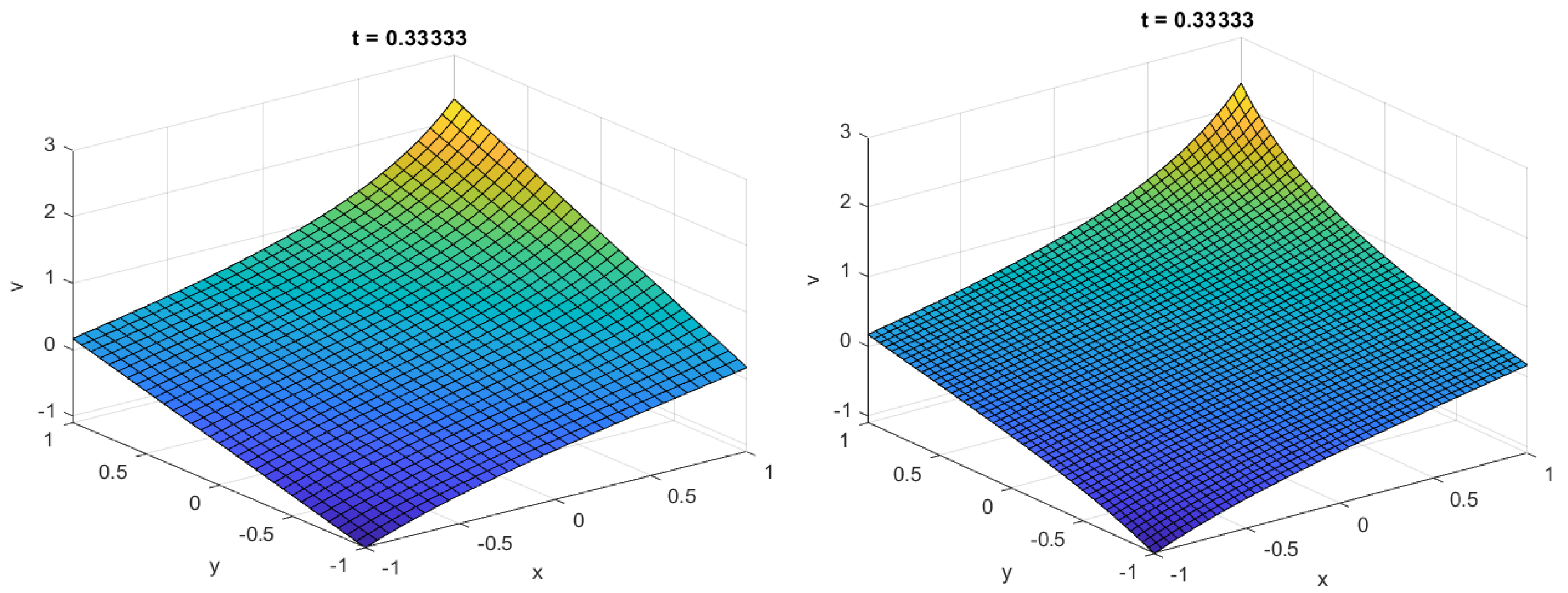
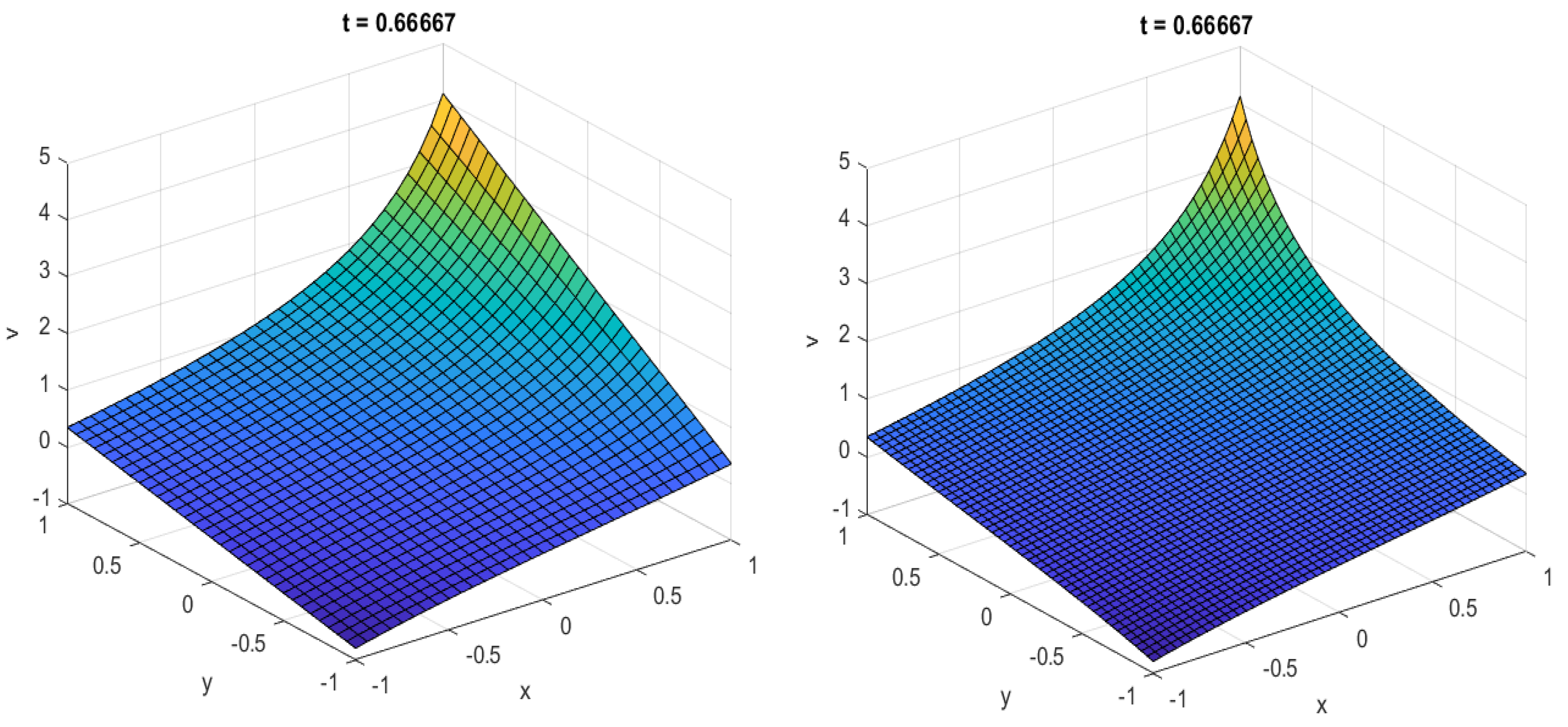
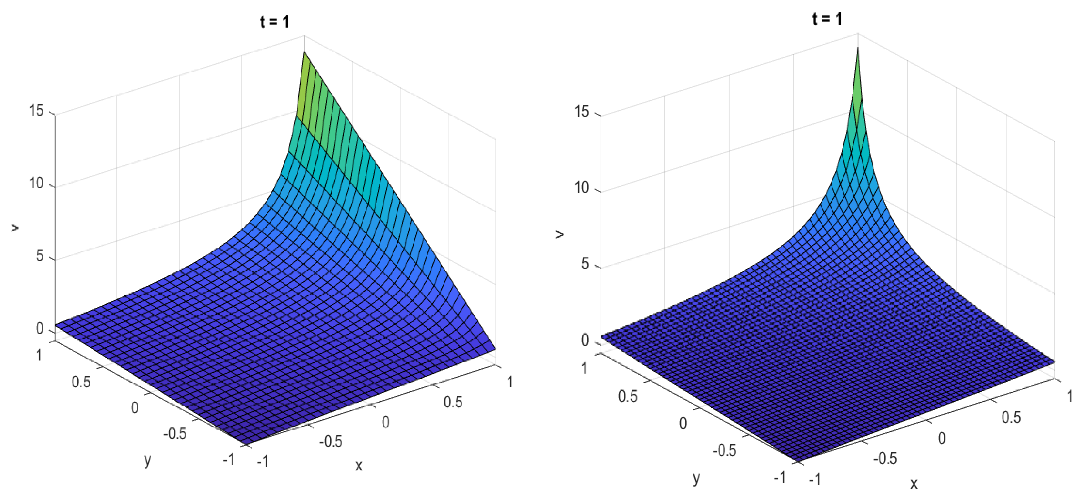
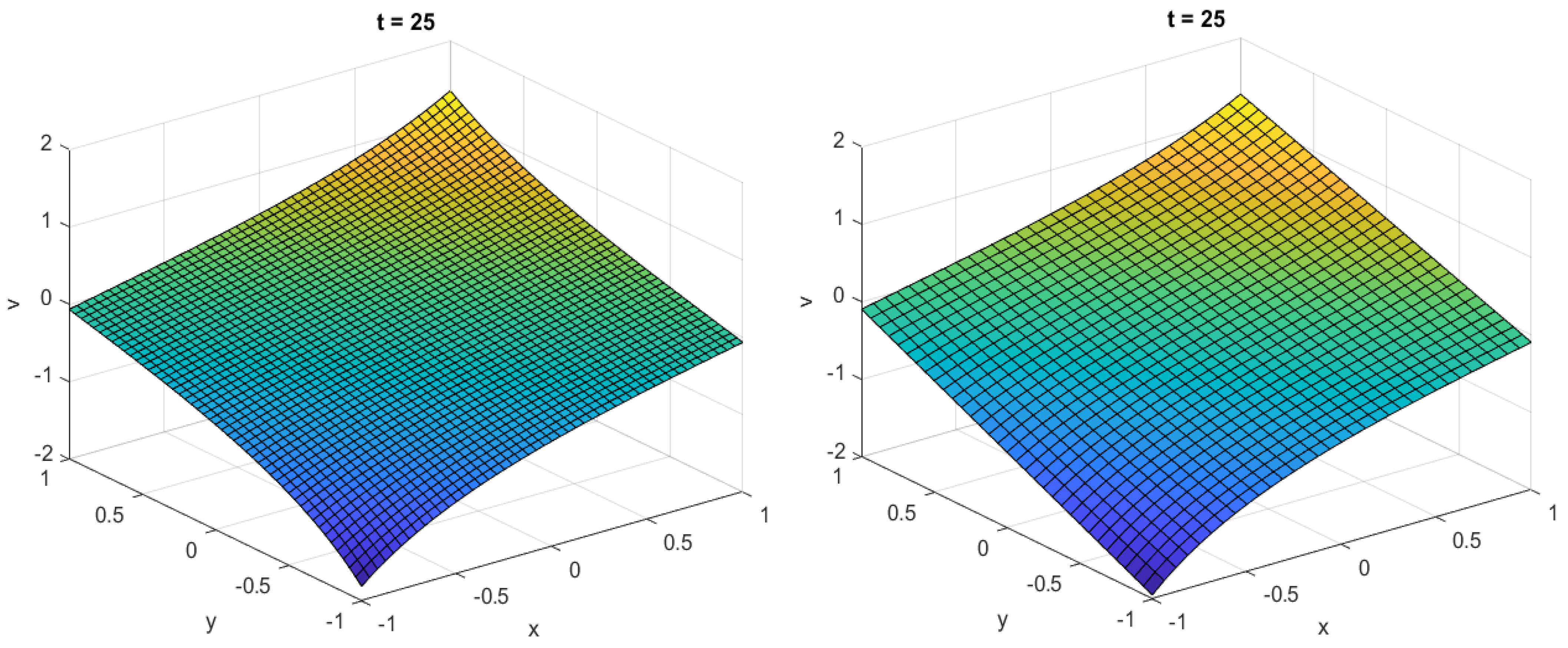
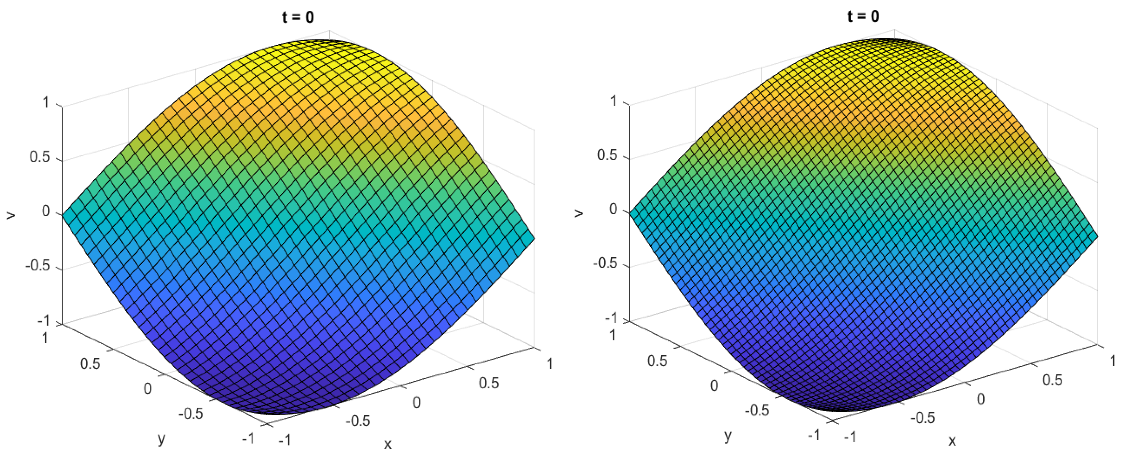
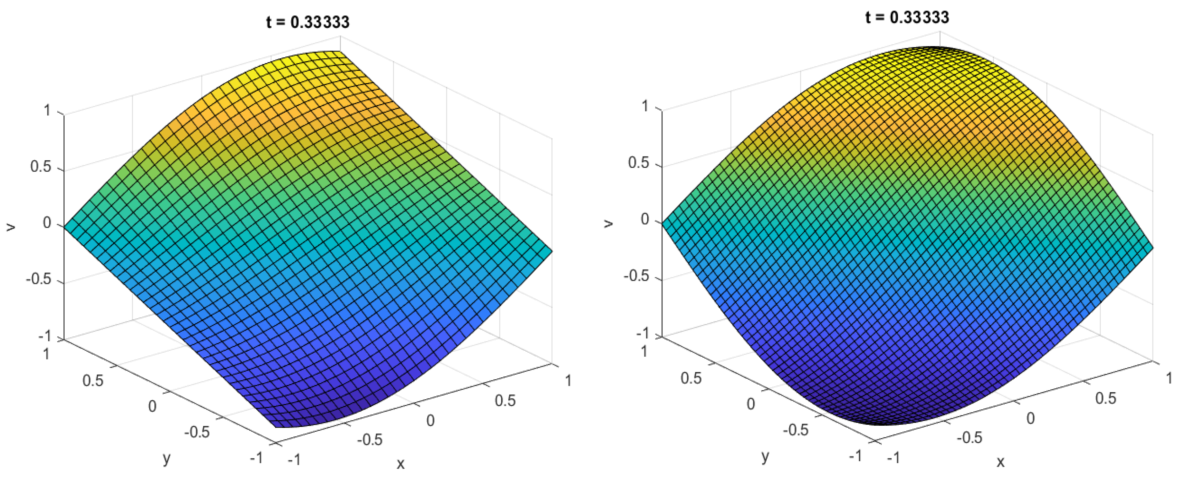
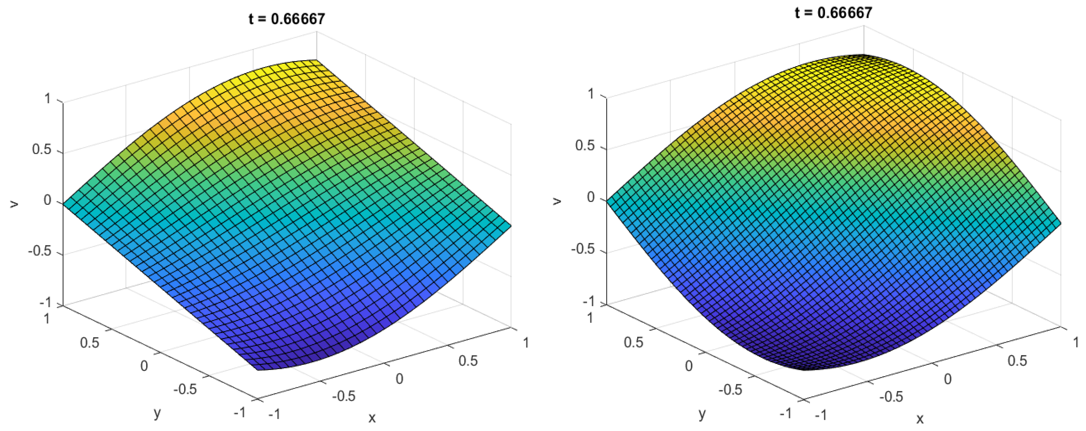
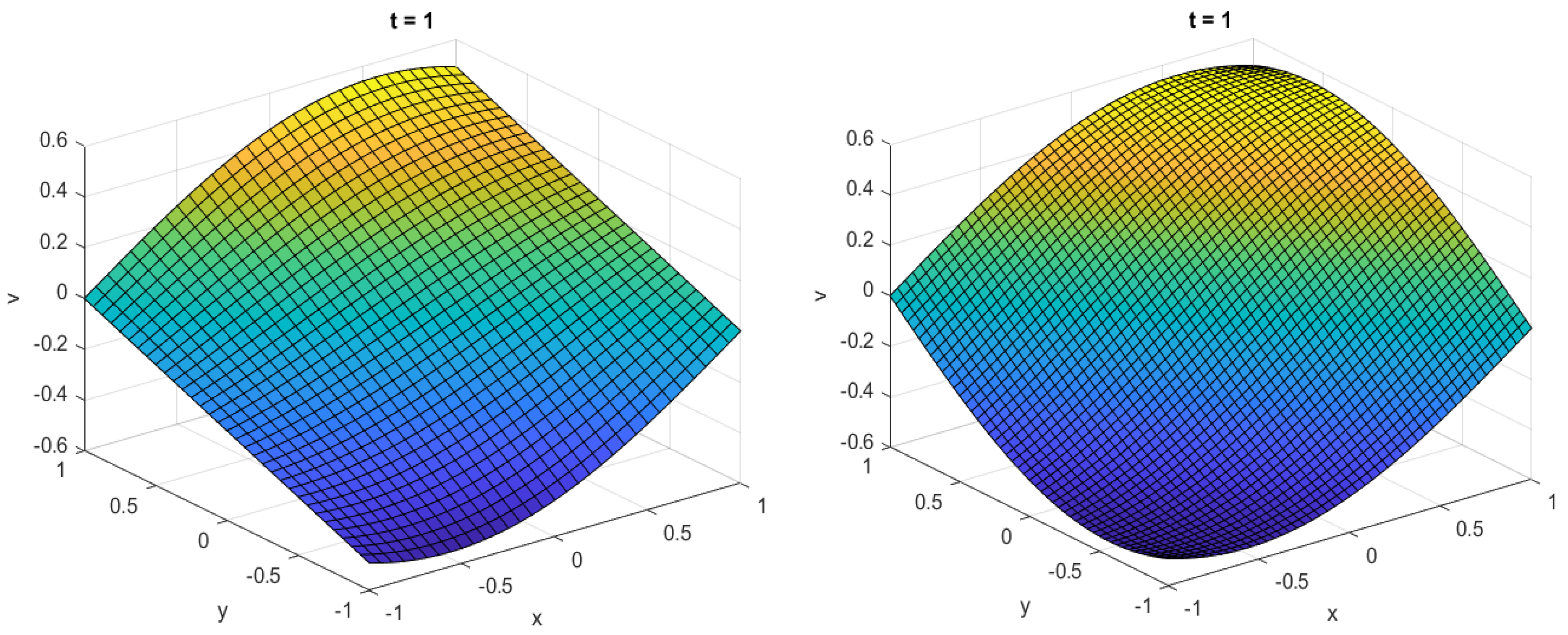
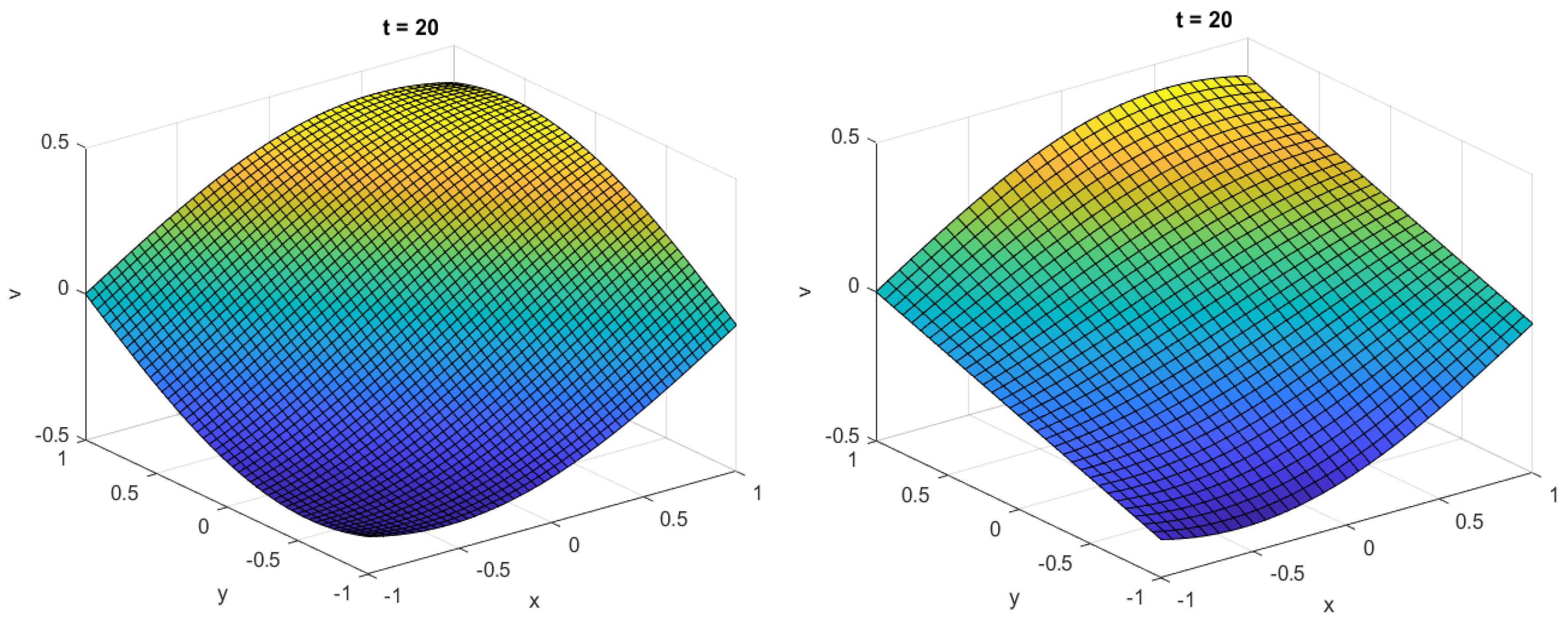
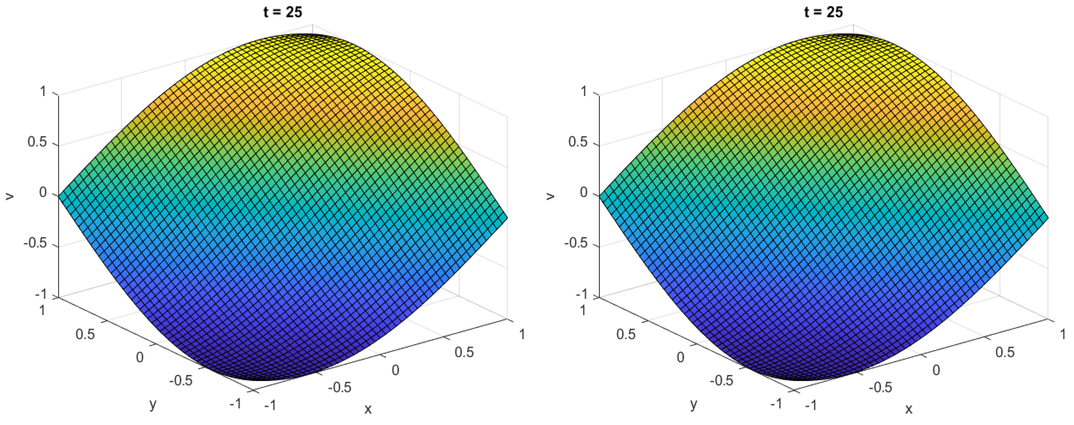
4. Numerical Examples

Two numerical examples of telegraph-type PDEs are presented in this section for the confirmation of the efficiency and the convergence rate, which are exponential using the method under consideration. The numerical solutions obtained were compared with their analytical counterparts for both lower and higher time steps to confirm the stability and accuracy. Figure 1, Figure 2, Figure 3, Figure 4, Figure 5 and Figure 6 show the comparison of the mentioned time steps, for example 1. Figure 7, Figure 8, Figure 9, Figure 10, Figure 11 and Figure 12 show the comparison, for example 2, with the exact solution. Table 1 and Table 2 represent the error behaviors of the exact and approximate solutions for using different norms for examples 1 and 2, respectively. From all these figures and tables, one can easily see the exponential rate of convergence for our scheme, the best possible one, which confirms the theoretical results given in the form of Theorems 1 and 2.

4.1. Example 1

Consider the following telegraph PDEs of hyperbolic type subject to appropriate initial and boundary conditions.

$$\begin{array}{c}\hfill v_{tt}+20v_t+25v=v_{xx}+v_{yy}+\xi se{c}^2\left(\frac{x+y+t}{2}\right)+{\eta }^{2}tan\left(\frac{x+y+t}{2}\right)\\ \hfill +se{c}^2\left(\frac{x+y+t}{2}\right)tan\left(\frac{x+y+t}{2}\right),\end{array}$$

(37)

subject to

$$\begin{array}{c}v(x,y,0)=tan\left(\frac{x+y}{2}\right)\\ \frac{\partial v}{\partial t}=\frac{1}{2}se{c}^2\left(\frac{x+y}{2}\right)\end{array}$$

(38)

$$\begin{array}{c}v(-1,y,t)=tan\left(\frac{t+y-1}{2}\right),\\ v(1,y,t)=tan\left(\frac{1+y+t}{2}\right),\\ v(x,-1,t)=tan\left(\frac{t+x-1}{2}\right),\\ v(x,1,t)=tan\left(\frac{1+x+t}{2}\right),\end{array}$$

(39)

for $\Delta t=0.0024,$ the exact solution for the corresponding equation is $v(x,y,t)=tan\left(\frac{x+y+t}{2}\right)$. Table 1 represents the error calculated with the comparison of analytical solutions at a different level of time. First, by keeping the time $t=0$, no error is computed because of the given initial conditions, but as the time increases, we find the error values, as shown in Table 1.

Table 1. Example 1: Exact vs. numerical solution error behavior.

Error	$\mathit{t}=0$	$\mathit{t}=0.333$	$\mathit{t}=0.666$	$\mathit{t}=1$	$\mathit{t}=20$	$\mathit{t}=25$
$L_{\infty }$	0	$8.6618\times {10}^{-16}$	$4.4409\times {10}^{-15}$	$4.2633\times {10}^{-14}$	$2.0250\times {10}^{-13}$	$4.0523\times {10}^{-15}$
$L_2$	0	$1.0671\times {10}^{-15}$	$6.0633\times {10}^{-15}$	$6.0120\times {10}^{-14}$	$2.0852\times {10}^{-13}$	$6.9549\times {10}^{-15}$
$L_1$	0	$2.9976\times {10}^{-15}$	$1.5501\times {10}^{-14}$	$1.0356\times {10}^{-13}$	$2.5224\times {10}^{-13}$	$1.2046\times {10}^{-14}$

Table 1. Example 1: Exact vs. numerical solution error behavior.

Error	$\mathit{t}=0$	$\mathit{t}=0.333$	$\mathit{t}=0.666$	$\mathit{t}=1$	$\mathit{t}=20$	$\mathit{t}=25$
$L_{\infty }$	0	$8.6618\times {10}^{-16}$	$4.4409\times {10}^{-15}$	$4.2633\times {10}^{-14}$	$2.0250\times {10}^{-13}$	$4.0523\times {10}^{-15}$
$L_2$	0	$1.0671\times {10}^{-15}$	$6.0633\times {10}^{-15}$	$6.0120\times {10}^{-14}$	$2.0852\times {10}^{-13}$	$6.9549\times {10}^{-15}$
$L_1$	0	$2.9976\times {10}^{-15}$	$1.5501\times {10}^{-14}$	$1.0356\times {10}^{-13}$	$2.5224\times {10}^{-13}$	$1.2046\times {10}^{-14}$

Figure 1. Example 1: Analytical (left) vs. approximate solution (right) at time $t=0$.

Figure 1. Example 1: Analytical (left) vs. approximate solution (right) at time $t=0$.

Figure 2. Example 1: Analytical (left) vs. approximate solution (right) at time $t=0.333$.

Figure 2. Example 1: Analytical (left) vs. approximate solution (right) at time $t=0.333$.

Figure 3. Example 1: Analytical (left) vs. approximate solution (right) at time $t=0.666$.

Figure 3. Example 1: Analytical (left) vs. approximate solution (right) at time $t=0.666$.

Figure 4. Example 1: Analytical (left) vs. approximate solution (right) at time $t=1.0$.

Figure 4. Example 1: Analytical (left) vs. approximate solution (right) at time $t=1.0$.

Figure 5. Example 1: Analytical (left) vs. approximate solution (right) at time $t=20$.

Figure 5. Example 1: Analytical (left) vs. approximate solution (right) at time $t=20$.

Figure 6. Example 1: Analytical (left) vs. approximate solution (right) at time $t=25$.

Figure 6. Example 1: Analytical (left) vs. approximate solution (right) at time $t=25$.

4.2. Example 2

Consider the following telegraph-type hyperbolic PDEs:

$$v_{tt}+20v_t+25v=v_{xx}+v_{yy}+(1+{\eta }^2)sin(x+y)cost-2\xi sin(x+y)sint,$$

(40)

subject to

$$\begin{array}{c}v(x,y,0)=sin(x+y)\\ \frac{\partial v(x,y,0)}{\partial t}=-sin(x+y)sint,\end{array}$$

(41)

$$\begin{array}{c}v(-1,y,t)=sin(y-1)cost,\\ v(1,y,t)=sin(1+y)cost,\\ v(x,-1,t)=sin(x-1)cost,\\ v(x,1,t)=sin(x+1)cost,\end{array}$$

(42)

for $\Delta t=0.0024,$ the exact solution for the corresponding equation is $v(x,y,t)=sin(x+y)cost$. Table 2 represents the error calculated with the comparison of analytical solutions at different levels of time. First, by keeping the time $t=0$, no error is computed because of the given initial conditions, but as the time increases, we find the error values, as shown in Table 2.

Table 2. Example 2: Exact and numerical solution error behavior.

Error	$\mathit{t}=0$	$\mathit{t}=0.333$	$\mathit{t}=0.666$	$\mathit{t}=1$	$\mathit{t}=20$	$\mathit{t}=25$
$L_{\infty }$	0	$3.2714\times {10}^{-12}$	$3.1828\times {10}^{-12}$	$8.4134\times {10}^{-12}$	$1.4094\times {10}^{-13}$	$1.1102\times {10}^{-14}$
$L_2$	0	$2.2305\times {10}^{-11}$	$4.2154\times {10}^{-11}$	$5.7362\times {10}^{-11}$	$9.6074\times {10}^{-13}$	$7.5708\times {10}^{-14}$
$L_1$	0	$1.5915\times {10}^{-10}$	$3.0079\times {10}^{-10}$	$4.0930\times {10}^{-10}$	$6.8553\times {10}^{-12}$	$5.4023\times {10}^{-13}$

Table 2. Example 2: Exact and numerical solution error behavior.

Error	$\mathit{t}=0$	$\mathit{t}=0.333$	$\mathit{t}=0.666$	$\mathit{t}=1$	$\mathit{t}=20$	$\mathit{t}=25$
$L_{\infty }$	0	$3.2714\times {10}^{-12}$	$3.1828\times {10}^{-12}$	$8.4134\times {10}^{-12}$	$1.4094\times {10}^{-13}$	$1.1102\times {10}^{-14}$
$L_2$	0	$2.2305\times {10}^{-11}$	$4.2154\times {10}^{-11}$	$5.7362\times {10}^{-11}$	$9.6074\times {10}^{-13}$	$7.5708\times {10}^{-14}$
$L_1$	0	$1.5915\times {10}^{-10}$	$3.0079\times {10}^{-10}$	$4.0930\times {10}^{-10}$	$6.8553\times {10}^{-12}$	$5.4023\times {10}^{-13}$

Figure 7. Example 2: Analytical (left) vs. approximate solution (right) at time $t=0$.

Figure 7. Example 2: Analytical (left) vs. approximate solution (right) at time $t=0$.

Figure 8. Example 2: Analytical (left) vs. approximate solution (right) at time $t=0.333$.

Figure 8. Example 2: Analytical (left) vs. approximate solution (right) at time $t=0.333$.

Figure 9. Example 2: Analytical (left) vs. approximate solution (right) at time $t=0.666$.

Figure 9. Example 2: Analytical (left) vs. approximate solution (right) at time $t=0.666$.

Figure 10. Example 2: Analytical (left) vs. approximate solution (right) at time $t=1.0$.

Figure 10. Example 2: Analytical (left) vs. approximate solution (right) at time $t=1.0$.

Figure 11. Example 2: Analytical (left) vs. approximate solution (right) at time $t=20$.

Figure 11. Example 2: Analytical (left) vs. approximate solution (right) at time $t=20$.

Figure 12. Example 2: Analytical (left) vs. approximate solution (right) at time $t=25$.

Figure 12. Example 2: Analytical (left) vs. approximate solution (right) at time $t=25$.

5. Conclusions

Special functions in the form of orthogonal functions based on Chebyshev polynomials have been used to find a robust and stable approximate solution of hyperbolic PDEs of telegraph type. The coefficients of a differentiation matrix obtained after discretizing the special part are efficiently evaluated using FFTs. It is shown that the error behaviors between the exact and numerical solutions using different norms decay exponentially. This means that one can achieve very high accuracy for a small number of collocation points. The proposed scheme is very simple, where the boundary conditions are automatically adjusted in the first and last row of the obtained differential matrix of Chebyshev polynomials. The theoretical justification of the error analysis has been confirmed through numerical simulations. We found that our numerical scheme has a very good agreement with the exact solution.

References

1. Canuto, H.; Quaterolli, Z. Spectral Methods; Springer: Berlin/Heidelberg, Germany, 2006. [Google Scholar]
2. Gottlieb, D.; Orszag, S.A. Numerical Analysis of Spectral Methods: Theory and Applications; SIAM: Philadelphia, PA, USA, 1977. [Google Scholar]
3. Trefethen, L.N. Spectral Methods in MATLAB; SIAM: Philadelphia, PA, USA, 2000. [Google Scholar]
4. Ali, I.; Khan, S.U. A Dynamic Competition Analysis of Stochastic Fractional Differential Equation Arising in Finance via Pseudospectral Method. Mathematics 2023, 11, 1328. [Google Scholar] [CrossRef]
5. Ali, I.; Saleem, M.T. Spatiotemporal Dynamics of Reaction-Diffusion System and Its Application to Turing Pattern Formation in a Gray-Scott Model. Mathematics 2023, 11, 1459. [Google Scholar] [CrossRef]
6. Khan, S.U.; Ali, M.; Ali, I. A spectral collocation method for stochastic Volterra integro-differential equations and its error analysis. Adv. Differ. Equ. 2019, 1, 161. [Google Scholar] [CrossRef] [Green Version]
7. Ali, A.; Khan, S.U.; Ali, I.; Khan, F.U. On dynamics of stochastic avian influenza model with asymptomatic carrier using spectral method. Math. Methods Appl. Sci. 2022, 45, 8230–8246. [Google Scholar] [CrossRef]
8. Khan, S.U.; Ali, I. Convergence and error analysis of a spectral collocation method for solving system of nonlinear Fredholm integral equations of second kind. Comput. Appl. Math. 2019, 38, 125. [Google Scholar] [CrossRef]
9. Dang, W.; Guo, J.; Liu, M.; Liu, S.; Yang, B.; Yin, L.; Zheng, W. A Semi-Supervised Extreme Learning Machine Algorithm Based on the New Weighted Kernel for Machine Smell. Appl. Sci. 2022, 12, 9213. [Google Scholar] [CrossRef]
10. Lu, S.; Guo, J.; Liu, S.; Yang, B.; Liu, M.; Yin, L.; Zheng, W. An Improved Algorithm of Drift Compensation for Olfactory Sensors. Appl. Sci. 2022, 12, 9529. [Google Scholar] [CrossRef]
11. Lu, S.; Ban, Y.; Zhang, X.; Yang, B.; Yin, L.; Liu, S.; Zheng, W. Adaptive control of time delay teleoperation system with uncertain dynamics. Front. Neurorobot. 2022, 16, 152. [Google Scholar] [CrossRef]
12. Ma, J.; Hu, J. Safe consensus control of cooperative-competitive multi-agent systems via differential privacy. Kybernetika 2022, 58, 426–439. [Google Scholar] [CrossRef]
13. Liu, Q.; Peng, H.; Wang, Z.-A. Convergence to nonlinear diffusion waves for a hyperbolic-parabolic chemotaxis system modelling vasculogenesis. J. Differ. Equ. 2022, 314, 251–286. [Google Scholar] [CrossRef]
14. Tautz, R.C.; Lerche, I. Application of the three-dimensional telegraph equation to cosmic-ray transport. Res. Astron. Astrophys. 2016, 16, 162. [Google Scholar] [CrossRef] [Green Version]
15. Debnath, L.; Mikusinski, P. Introduction to Hilbert Spaces with Applications; Academic Press: Cambridge, MA, USA, 2005. [Google Scholar]
16. El-Azab, M.S.; El-Gamel, M. A numerical algorithm for the solution of telegraph equations. Appl. Math. Comput. 2007, 190, 757–764. [Google Scholar] [CrossRef]
17. Patel, V.K.; Bahuguna, D. Numerical and approximate solutions for two-dimensional hyperbolic telegraph equation via wavelet matrices. Proc. Natl. Acad. Sci. India Sect. Phys. Sci. 2022, 92, 605–623. [Google Scholar] [CrossRef]
18. Metaxas, A.C.; Meredith, R.J. (Eds.) Industrial Microwave Heating; Peter Peregrinus Ltd.: London, UK, 1993. [Google Scholar]
19. Weston, V.H.; He, S. Wave splitting of the telegraph equation in R3and its application to inverse scattering. Inverse Probl. 1993, 9, 789. [Google Scholar] [CrossRef]
20. Banasiak, J.; Mika, J.R. Singularly perturved telegraph equations with applications in the random walk theory. J. Appl. Math. Stoch. Anal. 1998, 11, 9. [Google Scholar] [CrossRef] [Green Version]
21. Alpert, B.; Beylkin, G.; Gines, D.; Vozovoi, L. Adaptive solution of partial differential equations in multi-wavelet bases. J. Comput. Phys. 2002, 182, 149–190. [Google Scholar] [CrossRef] [Green Version]
22. Dehghan, M.; Saray, B.N.; Lakestani, M. Mixed finite difference and Galerkin methods for solving Burgers equations using interpolating scaling functions. Math. Method Appl. Sci. 2014, 37, 894–912. [Google Scholar] [CrossRef]
23. Hovhannisyan, N.; Muller, S.; Schafer, R. Adaptive multiresolution discontinuous Galerkin schemes—For conservation laws. Math. Comput. 2014, 83, 113–151. [Google Scholar] [CrossRef] [Green Version]
24. Saray, B.N.; Lakestani, M.; Cattani, C. Evaluation of mixed Crank-Nicolson scheme and Tau method for the solution of Klein-Gordon equation. Appl. Math. Comput. 2018, 331, 169–181. [Google Scholar]
25. Dehghan, M.; Mohammadi, V. Two numerical meshless techniques based on radial basis functions (RBFs) and the method of generalized moving least squares (GMLS) for simulation of coupled Klein Gordon Schrodinger (KGS) equations. Comput. Math. Appl. 2016, 71, 892–921. [Google Scholar] [CrossRef]
26. Chan, H.F.; Fan, C.M.; Kuo, C.W. Generalized finite difference method for solving two-dimensional non-linear obstacle problems. Eng. Anal. Bound. Elem. 2013, 37, 1189–1196. [Google Scholar] [CrossRef]
27. Dehghan, M.; Saadatmandi, A. Numerical solution of hyperbolic telegraph equation using the Chebyshev tau method. Numer. Methods Partial Differ. Equ. 2010, 26, 239–252. [Google Scholar]
28. Dehghan, M.; Ghesmati, A. Solution of the second-order one-dimensional hyperbolic telegraph equation by using the dual reciprocity boundary integral equation (DRBIE) method. Eng. Anal. Bound. Elem. 2010, 34, 51–59. [Google Scholar] [CrossRef]
29. Jiwari, R.; Pandit, S.; Mittal, R.C. A differential quadrature algorithm for solution of the second order one dimensional hyperbolic telegraph equation. For. Ecol. Manag. 2012, 249, 5–17. [Google Scholar]
30. Dehghan, M.; Ghesmati, A. Combination of meshless local weak and strong (MLWS) forms to solve the two dimensional hyperbolic telegraph equation. Eng. Anal. Bound. Elem. 2010, 34, 324–336. [Google Scholar] [CrossRef]
31. Xie, S.S.; Yi, S.C.; Kwon, T.I. Fourth-order compact difference and alternating direction implicit schemes for telegraph equations. Comput. Phys. Commun. 2012, 183, 552–569. [Google Scholar] [CrossRef]
32. Dehghan, M.; Satehi, R. A method based on meshless approach for the numerical solution of the two-space dimensional hyperbolic telegraph equation. Math. Methods Appl. Sci. 2012, 35, 220–1233. [Google Scholar] [CrossRef]
33. Lin, J.; Chen, F.; Zhang, Y.; Lu, J. An accurate meshless collocation technique for solving two- dimensional hyperbolic telegraph equations in arbitrary domains. Eng. Anal. Bound. Elem. 2019, 108, 372–384. [Google Scholar] [CrossRef]
34. Ding, H.; Zhang, Y.; Cao, J.; Tian, J. A class of difference scheme for solving telegraph equation by new non-polynomial spline methods. Appl. Math. Comput. 2012, 218, 4671–4683. [Google Scholar] [CrossRef]
35. Aloy, R.; Casaban, M.C.; Caudillo-Mata, L.A.; Jodar, L. Computing the variable coefficient telegraph equation using a discrete eigenfunctions method. Comput. Math. Appl. 2007, 54, 448–458. [Google Scholar] [CrossRef] [Green Version]
36. Biazar, J.; Eslami, M. Analytic solution for Telegraph equation by differential transform method. Phys. Lett. A 2010, 374, 2904–2906. [Google Scholar] [CrossRef]
37. Biazar, J.; Ebrahimi, H. An approximation to the solution of telegraph equation by adomian decomposition method. Int. Math. Forum 2007, 2, 2231–2236. [Google Scholar] [CrossRef] [Green Version]
38. Yao, H. Reproducing kernel method for the solution of nonlinear hyperbolic telegraph equation with an integral condition. Numer. Methods Partial Differ. Equ. 2011, 27, 867–886. [Google Scholar] [CrossRef]
39. Urena, F.; Gavete, L.; Benito, J.J.; Garcia, A.; Vargas, A.M. Solving the telegraph equation in 2-D and 3-D using generalized finite difference method (GFDM). Eng. Anal. Bound. Elem. 2020, 112, 13–24. [Google Scholar] [CrossRef]
40. Jebreen, H.B.; Cano, Y.C.; Dassios, I. An efficient algorithm based on the multi-wavelet Galerkin method for telegraph equation. AIMS Math. 2021, 6, 1296–1308. [Google Scholar] [CrossRef]
41. Kapoor, M.; Shah, N.A.; Saleem, S.; Weera, W. An Analytical Approach for Fractional Hyperbolic Telegraph Equation Using Shehu Transform in One, Two and Three Dimensions. Mathematics 2022, 10, 1961. [Google Scholar] [CrossRef]
42. Shah, N.A.; Dassios, I.; Chung, J.D. A Decomposition Method for a Fractional-Order Multi-Dimensional Telegraph Equation via the Elzaki Transform. Symmetry 2021, 13, 8. [Google Scholar] [CrossRef]
43. Dehghan, M.; Shokri, A. A numerical method for solving the hyperbolic telegraph equation. Numer. Methods Partial Differ. Equ. 2008, 24, 1080–1093. [Google Scholar] [CrossRef]
44. Bulbul, B.; Sezer, M. Taylor polynomial solution of hyperbolic type partial differential equations with constant coefficients. Int. J. Comput. 2011, 88, 533–544. [Google Scholar] [CrossRef]
45. Ding, H.; Zhang, Y. A new fourth-order compact finite difference scheme for the two-dimensional second-order hyperbolic equation. J. Comput. Appl. Math. 2009, 230, 626–632. [Google Scholar] [CrossRef] [Green Version]
46. Erdem Bicer, K.; Yalcinba, S. Numerical solution of telegraph equation using Bernoulli collocation method. Proc. Natl. Acad. Sci. India Sect. Phys. Sci. 2019, 89, 769–775. [Google Scholar] [CrossRef]
47. Javidi, M. Chebyshev Spectral Collocation Method for Computing Numerical Solution of Telegraph Equation. Comput. Methods Differ. Equ. 2013, 1, 16–29. [Google Scholar]
48. Karp, D.; Prilepkina, E. Beyond the Beta Integral Method: Transformation Formulas for Hypergeometric Functions via Meijer’s G Function. Symmetry 2022, 14, 1541. [Google Scholar] [CrossRef]
49. Ali, I.; Saleem, M.T. Applications of Orthogonal Polynomials in Simulations of Mass Transfer Diffusion Equation Arising in Food Engineering. Symmetry 2023, 15, 527. [Google Scholar] [CrossRef]
50. Sitnik, S.M.; Yadrikhinskiy, K.V.; Fedorov, V.E. Symmetry Analysis of a Model of Option Pricing and Hedging. Symmetry 2022, 14, 1841. [Google Scholar] [CrossRef]
51. Ali, I.; Khan, S.U. Asymptotic Behavior of Three Connected Stochastic Delay Neoclassical Growth Systems Using Spectral Technique. Mathematics 2022, 10, 3639. [Google Scholar] [CrossRef]
52. Ali, I.; Khan, S.U. Threshold of Stochastic SIRS Epidemic Model from Infectious to Susceptible Class with Saturated Incidence Rate Using Spectral Method. Symmetry 2022, 14, 1838. [Google Scholar] [CrossRef]
53. Ali, I.; Khan, S.U. Dynamics and simulations of stochastic COVID-19 epidemic model using Legendre spectral collocation method. AIMS Math. 2023, 8, 4220–4236. [Google Scholar] [CrossRef]
54. Caratelli, D.; Ricci, P.E. A Note on the Orthogonality Properties of the Pseudo-Chebyshev Functions. Symmetry 2020, 12, 1273. [Google Scholar] [CrossRef]
55. Reynolds, R.; Stauffer, A. A Note on the Summation of the Incomplete Gamma Function. Symmetry 2021, 13, 2369. [Google Scholar] [CrossRef]
56. Abd-Elhameed, W.M.; Alkhamisi, S.O. New Results of the Fifth-Kind Orthogonal Chebyshev Polynomials. Symmetry 2021, 13, 2407. [Google Scholar] [CrossRef]
57. Heideman, M.T.; Johnson, D.H.; Burrus, C.S. Gauss and the history of the fast Fourier transform. Arch. Hist. Exact Sci. 1985, 34, 265–277. [Google Scholar] [CrossRef] [Green Version]
58. Mastroianni, G.; Occorsio, D. Optional systems of nodes for Lagrange interpolation on bounded intervals. J. Comput. Appl. Math. 2001, 134, 325–341. [Google Scholar] [CrossRef] [Green Version]
Disclaimer/Publisher’s Note: The statements, opinions and data contained in all publications are solely those of the individual author(s) and contributor(s) and not of MDPI and/or the editor(s). MDPI and/or the editor(s) disclaim responsibility for any injury to people or property resulting from any ideas, methods, instructions or products referred to in the content.