Geometric Aggregation Operators for Solving Multicriteria Group Decision-Making Problems Based on Complex Pythagorean Fuzzy Sets

Abstract

The Complex Pythagorean fuzzy set (CPyFS) is an efficient tool to handle two-dimensional periodic uncertain information, which has various applications in fuzzy modeling and decision making. It is known that the aggregation operators influence decision-making processes. Algebraic aggregation operators are the important and widely used operators in decision making techniques that deal with uncertain problems. This paper investigates some complex Pythagorean fuzzy geometric aggregation operators, such as complex Pythagorean fuzzy weighted geometric (CPyFWG), complex Pythagorean fuzzy ordered weighted geometric (CPyFOWG), complex Pythagorean fuzzy hybrid geometric (CPyFHG), induced complex Pythagorean fuzzy ordered weighted geometric (I-CPyFOWG), and induced complex Pythagorean fuzzy hybrid geometric (I-CPyFHG), and their structure properties, such as idempotency, boundedness, and monotonicity. In addition, we compare the proposed model with their existing models, such as complex fuzzy set and complex intuitionistic fuzzy set. We analyze an example involving the selection of an acceptable location for hospitals in order to demonstrate the effectiveness, appropriateness, and efficiency of the novel aggregation operators.

1. Introduction

Decision making is the procedure in which experts assess the performance of alternatives based on a set of criteria to select the most optimal alternative. Making decisions is one of the best ways to sort through a selection of choices and pick the best one. In the past, it has been widely believed that all the data pertaining and relating to the alternative’s criteria and associated weights are given as clear numbers. However, most decisions in the real world are made in environments where aims and restrictions are often unclear or not well-defined.

To deal with these real-life situations, Zadeh [1] introduced the idea of the fuzzy set (FS), which has only one component called the membership grade (MEG) and describes the level of satisfaction of an object without disclosing the object’s dissatisfaction. Thus, scholars have not considered dissatisfaction independently. For example, if an element’s satisfaction is $0.3$, then its dissatisfaction should be considered as $1-0.3=0.7$. In order to address this weakness, Atanassov [2] presented the theory of intuitionistic fuzzy set (IFSs) by impressing each element in the form order, such that: $\left(Ъ,ф\right)$ where $Ъ$, $ф$ respectively, stand for membership grade (MeG) and non-membership grade (NMeG) under restriction, such as $0\prec Ъ+ф\le 1$. So, IFS is the most effective model for addressing the problems in comparison to fuzzy set. However, the selected model has some weaknesses. For example, if $Ъ=0.7$, $ф=0.6$, then $Ъ+ф=0.7+0.6=1.3\succ 1$. Thus, IFS is unable to solve these problems. Later on, Yager [3] extended the commencement of IFSs to Pythagorean fuzzy sets (PyFS), which relaxes the limitation of IFS to $0\prec {Ъ}^2+{ф}^2\le 1$. Hence, PFS is a more powerful tool for decision making compared to IFS. However, the proposed model has some weaknesses. For example, if $Ъ=0.8,ф=0.8$, then ${Ъ}^2+{ф}^2={\left(0.8\right)}^2+{\left(0.8\right)}^2=64+64=1.28\succ 1$. Senapati and Yager [4] extended PyFS to Fermatean fuzzy sets (FeFS), which reduces the limitation of PyFS to $0\prec {Ъ}^3+{ф}^3\le 1$. Thus, Fermatean fuzzy set is the more powerful tool for decision making compared to the IF environment and PyFS environment.

The most striking and imperative tools for handling decision cases in an IF environment, PyF environment, and FeF environment are aggregation operators. Several researchers studied the prominence of operators related to the IF environment in [5,6,7,8,9,10] and presented many operators with this domain for different challenges. Ahmmad et al. [11] introduced the Intuitionistic Fuzzy Rough Aczel-Alsina Aggregation Operators. Rahman et al. [12,13,14,15] studied various methods in the PyF environment, such as PFWG operator, PFOWG operator, PFHG operator, PFWA operator, PFOWA operator, and PFHA operator. Garg [16,17] settled Einstein arithmetic and Einstein geometric methods under PyFNs and proved their advantages, compensations, and applications. Zulqarnain et al. [18,19,20] introduced PFSEOWA operator, PFSEOWG operator, and PFSEWA operator, respectively, and also applied them to a group decision making problem. Zulqarnain and Dayan [21] introduced the Topsis method under the intuitionistic fuzzy environment.

These methods are unable to describe the partial ignorance of the data and their volatility throughout a specific time period, according to the literature study mentioned above. As a result, only non-periodic information may be handled by any of the FS theory extensions indicated above. However, in complex data sets, ambiguity and vagueness also coexist with changes to the periodicity of the data. For instance, complex data sets may contain substantial amounts of information from various sources, such as government biometric databases, audio, image analysis, facial recognition, and medical research. These databases also contain a lot of contradictory and incomplete information. To avoid these situations, Ramot et al. [22] presented the idea of complex fuzzy set (CFS), where the complex membership grade (CMEG) is represented by complex fuzzy numbers (CFNs) instead of real integers in the unit circle. Later on, Alkouri and Salleh [23] generalized this idea by introducing the idea of complex intuitionistic fuzzy set (CIFS), based on the complex membership grade (CMEG) $Ъe^{iл}$ and complex non-membership grade (CNMEG) $фe^{i\tau }$ with environment, such as $0\prec Ъ+ф\le 1$ and $0\le \frac{л}{2\pi }+\frac{\tau }{2\pi }\le 1$, where $0\prec Ъ,ф\le 1$, $л,\tau \in \left[0, 2\pi \right]$. Later, Ma et al. [24] used CFNs and presented a new method to address multi-periodic factors, called the CFS-based method. Dick et al. [25] have published several applicable and important laws addressing the decision-making problems. The results of [26] were modified by Liu and Zhang [27] and presented in a brand new, sophisticated manner. Garg and Rani [28], Kumar and Bajaj [29], and Rani and Garg [30] studied different types of aggregation operators in CIF environments. Greenfield et al. [31] introduced the idea of complex interval-valued fuzzy set (CIVFSs). Garg and Rani [32] presented the idea of robust correlation coefficient and their applications in decision making under complex intuitionistic fuzzy numbers. Later on, Ullah et al. [33] extended the notion of CIFS to the complex Pythagorean fuzzy set (CPyFS), which reduces and relaxes the limitation and drawback of CIFS. CPFS is also based on the complex value membership grade $Ъe^{iл}$ and complex value non-membership grade $фe^{i\tau }$ under restriction, such as $0\prec {Ъ}^2+{ф}^2\le 1$ and $0\prec {\left(\frac{л}{2\pi }\right)}^2+{\left(\frac{\tau }{2\pi }\right)}^2\le 1$, where $Ъ,ф \left[0,1\right]$ and $л,\tau \in \left[0,2\pi \right]$. Liu et al. [29] presented the idea of complex q-rung orthopair fuzzy sets and developed several aggregation operators using the proposed model. Some related work is found in [34,35,36,37]. Ali et al. [38] introduced several complex interval-valued Pythagorean fuzzy geometric aggregation operators and their application to decision making problems. Rahman et al. [39] and Rahman and Iqbal [40] introduced a set of aggregation operators based on complex Pythagorean fuzzy numbers and applied them to the group decision making problem.

Motivated by [39], where the authors developed several arithmetic aggregation operators, such as the CPyFWA operator, the CPyFOWA operator, the CPyFHA operator, the I-CPyFOWA operator, and the I-CPyFHA operator and applied them to the decision-making problem. However, we know that geometric aggregation operators are a good alternative to arithmetic aggregation operators. Therefore, in this paper, we introduce some geometric aggregation operators, namely the CPyFWG operator, the CPyFOWG operator, the CPyFHG operator, the I-CPyFOWG operator, and the I-CPyFHG operator, along with examples, properties, and application.

The following paper is planned as follows. Section 2 presents fundamental definitions and Section 3 presents basic operation laws under CPyFNs. In Section 4, different operators under the CPyF environment are studied. Section 5 includes an emergency decision-making model under the novel approach. Section 6 provides an illustrative example under different techniques. Section 7 presents a comparative analysis. Section 8 presents a sensitivity analysis. Finally, Section 9 presents the conclusion.

2. Preliminaries

Definition 1

[22]. Let $\AE$ be the complex fuzzy set defined on the finite fixed universal set $\yen$ as: with condition, such that , and then ${Ъ}_{\AE }\left(c\right)$ is called the CMeG of $c$ with $i=\sqrt{-1}$ and ${л}_{\AE }\left(c\right)$ be the function of the real value.

Definition 2

[23]. Let $Ï$ be the complex intuitionistic fuzzy set defined on the finite fixed universal set $\yen$ as: , where $i=\sqrt{-1}$, ${Ъ}_{Ï}\left(c\right)\in [0,1]$ ${ф}_{Ï}\left(c\right)\in [0,1]$ are called the CMeG and the CNMeG of $c$, respectively, with situation, such as $0\prec {Ъ}_{Ï}\left(c\right)+{ф}_{Ï}\left(c\right)\le 1$. Moreover, ${л}_{Ï}\left(c\right)\in [0,2\pi ]$ and ${\tau }_{Ï}\left(c\right)\in [0,2\pi ]$ with restriction, such as, $0\prec \frac{{л}_{Ï}\left(c\right)}{2\pi }+\frac{{\tau }_{Ï}\left(c\right)}{2\pi }\le 1$, .

Definition 3

[32]. Let $\mathfrak{M}$ be the complex Pythagorean fuzzy set defined on the finite fixed universal set $\yen$ as: , $i=\sqrt{-1}$, ${Ъ}_{\mathfrak{M}}\left(c\right)\in [0,1],{ф}_{\mathfrak{M}}\left(c\right)\in [0,1]$, are called the CMeG and the CNMeG of, $c$ respectively, with condition, such as $0\prec {\left({Ъ}_{\mathfrak{M}}\left(c\right)\right)}^2+{\left({ф}_{\mathfrak{M}}\left(c\right)\right)}^2\le 1$. Moreover, ${л}_{\mathfrak{M}}\left(c\right)\in [0,2\pi ]$ and ${\tau }_{\mathfrak{M}}\left(c\right)\in [0,2\pi ]$ with $0\prec {\left(\frac{{л}_{\mathfrak{M}}\left(c\right)}{2\pi }\right)}^2+{\left(\frac{{\tau }_{\mathfrak{M}}\left(c\right)}{2\pi }\right)}^2\le 1$, .

Definition 4

[35]. Let $Ћ=\left(Ъe^{iл},фe^{i\tau }\right)$ be a CPyFN, then its score and accuracy are given by: $Sc\left(Ћ\right)=\left({Ъ}^2-{ф}^2\right)+\frac{1}{4{\pi }^2}\left({л}^2-{\tau }^2\right)$ and $Ac\left(Ћ\right)=\left({Ъ}^2+{ф}^2\right)+\frac{1}{4{\pi }^2}\left({л}^2+{\tau }^2\right)$ with $Sc\left(Ћ\right)\in \left[-2,2\right],Ac\left(Ћ\right)\in \left[0,2\right]$, respectively.

Definition 5

[35]. Let ${Ћ}_j=\left({Ъ}_j{e}^{i{л}_j},{ф}_j{e}^{i{\tau }_j}\right)\left(1\le j\le 2\right)$ be group of CPyFNs, then

(1)

If,$Sc\left({Ћ}_1\right)\succ Sc\left({Ћ}_2\right)\iff {Ћ}_1\succ {Ћ}_2$

(2)

If,$Sc\left({Ћ}_1\right)\prec Sc\left({Ћ}_2\right)\iff {Ћ}_1\prec {Ћ}_2$, then${Ћ}_1\prec {Ћ}_2$

(3)

If,$Sc\left({Ћ}_1\right)=Sc\left({Ћ}_2\right)$, then there are three conditions:

(i)

If,$Ac\left({Ћ}_1\right)\succ Ac\left({Ћ}_2\right)\iff {Ћ}_1\succ {Ћ}_2$

(ii)

If,$Ac\left({Ћ}_1\right)\prec Ac\left({Ћ}_2\right)\iff {Ћ}_1\prec {Ћ}_2$

(iii)

If,$Ac\left({Ћ}_1\right)=Ac\left({Ћ}_2\right)\iff {Ћ}_1={Ћ}_2$

3. Basic Operations under CPyFNs

Definition 6.

Let${Ћ}_j=\left({Ъ}_j{e}^{i{л}_j},{ф}_j{e}^{i{\tau }_j}\right)\left(1\le j\le 2\right)$be a family of CPyFNs, then

(i)

${Ћ}_1\oplus {Ћ}_2=\left(\sqrt{{Ъ}_1^2+{Ъ}_2^2-{Ъ}_1^2{Ъ}_2^2}{e}^{i2\pi \sqrt{{\left(\frac{{л}_1}{2\pi }\right)}^2+{\left(\frac{{л}_2}{2\pi }\right)}^2-{\left(\frac{{л}_1}{2\pi }\right)}^2{\left(\frac{{л}_2}{2\pi }\right)}^2}},\left({ф}_1{ф}_2\right)e^{\left(\frac{{\tau }_1}{2\pi }\right)\left(\frac{{\tau }_2}{2\pi }\right)}\right)$

(ii)

${Ћ}_1\otimes {Ћ}_2=\left(\left({Ъ}_1{Ъ}_2\right)e^{\left(\frac{{л}_1}{2\pi }\right)\left(\frac{{л}_2}{2\pi }\right)},\sqrt{{ф}_1^2+{ф}_2^2-{ф}_1^2{ф}_2^2}{e}^{i2\pi \sqrt{{\left(\frac{{\tau }_1}{2\pi }\right)}^2+{\left(\frac{{\tau }_2}{2\pi }\right)}^2-{\left(\frac{{\tau }_1}{2\pi }\right)}^2{\left(\frac{{\tau }_2}{2\pi }\right)}^2}}\right)$

(iii)

$\varrho \left({Ћ}_1\right)=\left(\sqrt{1-{\left(1-{Ъ}_1^2\right)}^{\varrho }}{e}^{\sqrt[i2\pi ]{1-{\left(1-{\left(\frac{{л}_1}{2\pi }\right)}^2\right)}^{\varrho }}},{\left({ф}_1\right)}^{\varrho }{e}^{i2\pi {\left(\frac{{\tau }_1}{2\pi }\right)}^{\varrho }}\right)$

(iv)

${\left({Ћ}_1\right)}^{\varrho }=\left({\left({Ъ}_1\right)}^{\varrho }{e}^{i2\pi {\left(\frac{{л}_1}{2\pi }\right)}^{\varrho }},\sqrt{1-{\left(1-{ф}_1^2\right)}^{\varrho }}{e}^{\sqrt[i2\pi ]{1-{\left(1-{\left(\frac{{\tau }_1}{2\pi }\right)}^2\right)}^{\varrho }}}\right)$

Example 1.

To develop the above definition, here we consider an example. Let${Ћ}_1=\left(0.7e^{i2\pi \left(0.6\right)},0.3e^{i2\pi \left(0.5\right)}\right)$and${Ћ}_2=\left(0.6e^{i2\pi \left(0.5\right)},0.5e^{i2\pi \left(0.3\right)}\right)$and$\varrho =2$, then

$$\begin{array}{l}{Ћ}_1\oplus {Ћ}_2\\ =\left(\sqrt{{\left(0.7\right)}^2+{\left(0.6\right)}^2-{\left(0.7\right)}^2{\left(0.6\right)}^2} e^{i2\pi \sqrt{{\left(\frac{0.6}{2\pi }\right)}^2+{\left(\frac{0.5}{2\pi }\right)}^2-{\left(\frac{0.6}{2\pi }\right)}^2{\left(\frac{0.5}{2\pi }\right)}^2}},\left(0.3\right)\left(0.5\right)e^{\left(\frac{0.5}{2\pi }\right)\left(\frac{0.3}{2\pi }\right)}\right)\\ =\left(0.78e^{i2\pi \left(0.69\right)},0.15e^{i2\pi \left(0.15\right)}\right)\\ {Ћ}_1\otimes {Ћ}_2\\ =\left(\left(0.7\right)\left(0.6\right)e^{\left(\frac{0.6}{2\pi }\right)\left(\frac{0.5}{2\pi }\right)},\sqrt{{\left(0.3\right)}^2+{\left(0.5\right)}^2-{\left(0.3\right)}^2{\left(0.5\right)}^2}{e}^{i2\pi \sqrt{{\left(\frac{0.5}{2\pi }\right)}^2+{\left(\frac{0.3}{2\pi }\right)}^2-{\left(\frac{0.5}{2\pi }\right)}^2{\left(\frac{0.3}{2\pi }\right)}^2}}\right)\\ =\left(0.42e^{i2\pi \left(0.30\right)},0.56e^{i2\pi \left(0.56\right)}\right)\\ {}^{\varrho }\left(Ћ\right)=\left(\sqrt{1-{\left(1-{\left(0.7\right)}^2\right)}^2}{e}^{\sqrt[i2\pi ]{1-{\left(1-{\left(\frac{0.6}{2\pi }\right)}^2\right)}^2}},{\left(0.3\right)}^2{e}^{i2\pi {\left(\frac{0.5}{2\pi }\right)}^2}\right)=\left(\begin{array}{l}0.86e^{i2\pi \left(0.76\right)},\\ 0.09e^{i2\pi \left(0.25\right)}\end{array}\right)\\ {\left(Ћ\right)}^{\varrho }=\left({\left(0.7\right)}^2{e}^{i2\pi {\left(\frac{0.6}{2\pi }\right)}^2},\sqrt{1-{\left(1-{\left(0.3\right)}^2\right)}^2}{e}^{\sqrt[i2\pi ]{1-{\left(1-{\left(\frac{0.5}{2\pi }\right)}^2\right)}^2}}\right)=\left(\begin{array}{l}0.49e^{i2\pi \left(0.36\right)},\\ 0.41e^{i2\pi \left(0.66\right)}\end{array}\right)\end{array}$$

Theorem 1.

Let${Ћ}_j=\left({Ъ}_j{e}^{i{л}_j},{ф}_j{e}^{i{\tau }_j}\right)\left(1\le j\le 2\right)$be a family of CPyFNs, then

1.

Symmetry property of score function: Let ${Ћ}_j=\left({Ъ}_j{e}^{i{л}_j},{ф}_j{e}^{i{\tau }_j}\right)\left(1\le j\le 2\right)$ be a group of CPyFNs, and let ${\left({Ћ}_j\right)}^c=\left({ф}_j{e}^{i{\tau }_j},{Ъ}_j{e}^{i{л}_j}\right)\left(1\le j\le 2\right)$ be their corresponding complements, then $Sc\left({Ћ}_1\right)\le Sc\left({Ћ}_2\right)\iff Sc{\left({Ћ}_1\right)}^c\ge Sc{\left({Ћ}_2\right)}^c$.

Proof. 

As $Sc\left({Ћ}_1\right)=\left({Ъ}_1^2-{ф}_1^2\right)+\frac{1}{4{\pi }^2}\left({л}_1^2-{\tau }_1^2\right)$ and $Sc\left({Ћ}_2\right)=\left({Ъ}_2^2-{ф}_2^2\right)+\frac{1}{4{\pi }^2}\left({л}_2^2-{\tau }_2^2\right)$. □

Now by Definition 4, we have $Sc\left({Ћ}_1\right)\le Sc\left({Ћ}_2\right)$, then

$$\begin{array}{l}\iff Sc\left({Ћ}_1\right)=\left({Ъ}_1^2-{ф}_1^2\right)+\frac{1}{4{\pi }^2}\left({л}_1^2-{\tau }_1^2\right)\le Sc\left({Ћ}_2\right)=\left({Ъ}_2^2-{ф}_2^2\right)+\frac{1}{4{\pi }^2}\left({л}_2^2-{\tau }_2^2\right)\\ \iff Sc\left({Ћ}_1\right)=\left(-{Ъ}_1^2+{ф}_1^2\right)+\frac{1}{4{\pi }^2}\left(-{л}_1^2+{\tau }_1^2\right)\ge Sc\left({Ћ}_2\right)=\left(-{Ъ}_2^2+{ф}_2^2\right)+\frac{1}{4{\pi }^2}\left(-{л}_2^2+{\tau }_2^2\right)\\ \iff Sc\left({Ћ}_1\right)=\left({ф}_1^2-{Ъ}_1^2\right)+\frac{1}{4{\pi }^2}\left({\tau }_1^2-{л}_1^2\right)\ge Sc\left({Ћ}_2\right)=\left({ф}_2^2-{Ъ}_2^2\right)+\frac{1}{4{\pi }^2}\left({\tau }_2^2-{л}_2^2\right)\\ \iff Sc{\left({Ћ}_1\right)}^c\ge Sc{\left({Ћ}_2\right)}^c\end{array}$$

2.

Monotonicity property of score functions: If $Ћ=\left(Ъe^{iл},фe^{i\tau }\right)$ be a CPyFN, then $Sc\left(Ћ\right)=\left({Ъ}^2-{ф}^2\right)+\frac{1}{4{\pi }^2}\left({л}^2-{\tau }^2\right)$ is monotonically decreasing when $ф,\tau$ are increasing and monotonically increasing with $Ъ$ and $л$ decreasing.

Proof. 

The proof is simple; so it is omitted here. □

3.

Symmetry property of accuracy function: If $Ћ=\left(Ъe^{iл},фe^{i\tau }\right)$ be a CPyFN and ${Ћ}^c=\left(фe^{i\tau },Ъe^{iл}\right)$ be their corresponding complement function, then $Ac\left(Ћ\right)=Ac{\left(Ћ\right)}^c$.

Proof. 

Since $Sc\left(Ћ\right)=\left({Ъ}^2-{ф}^2\right)+\frac{1}{4{\pi }^2}\left({л}^2-{\tau }^2\right)$. As $Ac\left(Ћ\right)=Ac{\left(Ћ\right)}^c$, then we have $Ac\left(Ћ\right)=\left({Ъ}^2+{ф}^2\right)+\frac{1}{4{\pi }^2}\left({л}^2+{\tau }^2\right)=\left({ф}^2+{Ъ}^2\right)+\frac{1}{4{\pi }^2}\left({\tau }^2+{л}^2\right)=Ac{\left(Ћ\right)}^c$. □

4.

Monotonicity property of accuracy functions: If $Ћ=\left(Ъe^{iл},фe^{i\tau }\right)$ be a CPyFN, then the accuracy function $Ac\left(Ћ\right)=\left({Ъ}^2+{ф}^2\right)+\frac{1}{4{\pi }^2}\left({л}^2+{\tau }^2\right)$ is monotonically increasing with the terms $Ъ,л,ф$ and $\tau$ are increasing.

Proof. 

The proof is simple; so it is omitted here. □

Theorem 2.

Let${Ћ}_j=\left({Ъ}_j{e}^{i{л}_j},{ф}_j{e}^{i{\tau }_j}\right)\left(1\le j\le 3\right)$be a family of CPyFNs, then

(1)

Commutative laws:

(i)

${Ћ}_1\oplus {Ћ}_2={Ћ}_2\oplus {Ћ}_1$

(ii)

${Ћ}_1\otimes {Ћ}_2={Ћ}_2\otimes {Ћ}_1$

(2)

Associative laws:

(i)

$\left({Ћ}_1\oplus {Ћ}_2\right)\oplus {Ћ}_3={Ћ}_1\oplus \left({Ћ}_2\oplus {Ћ}_3\right)$

(ii)

$\left({Ћ}_1\otimes {Ћ}_2\right)\otimes {Ћ}_3={Ћ}_1\otimes \left({Ћ}_2\otimes {Ћ}_3\right)$

(3)

Distributive laws:

(i)

${Ћ}_1\otimes \left({Ћ}_2\oplus {Ћ}_3\right)={Ћ}_1\otimes {Ћ}_2\oplus {Ћ}_1\otimes {Ћ}_3$

(ii)

$\left({Ћ}_1\oplus {Ћ}_2\right)\otimes {Ћ}_3={Ћ}_1\otimes {Ћ}_3\oplus {Ћ}_2\otimes {Ћ}_3$

Proof. 

We prove only 1, and the remaining parts can be proved by the same process.

$$\begin{array}{ll}{Ћ}_1\oplus {Ћ}_2& =\left(\sqrt{{Ъ}_1^2+{Ъ}_2^2-{Ъ}_1^2{Ъ}_2^2}{e}^{i2\pi \sqrt{{\left(\frac{{л}_1}{2\pi }\right)}^2+{\left(\frac{{л}_2}{2\pi }\right)}^2-{\left(\frac{{л}_1}{2\pi }\right)}^2{\left(\frac{{л}_2}{2\pi }\right)}^2}},\left({ф}_1{ф}_2\right)e^{\left(\frac{{\tau }_1}{2\pi }\right)\left(\frac{{\tau }_2}{2\pi }\right)}\right)\\ & =\left(\sqrt{{Ъ}_2^2+{Ъ}_1^2-{Ъ}_2^2{Ъ}_1^2}{e}^{i2\pi \sqrt{{\left(\frac{{л}_2}{2\pi }\right)}^2+{\left(\frac{{л}_1}{2\pi }\right)}^2-{\left(\frac{{л}_2}{2\pi }\right)}^2{\left(\frac{{л}_1}{2\pi }\right)}^2}},\left({ф}_2{ф}_1\right)e^{\left(\frac{{\tau }_2}{2\pi }\right)\left(\frac{{\tau }_1}{2\pi }\right)}\right)\\ & ={Ћ}_2\oplus {Ћ}_1\\ {Ћ}_1\otimes {Ћ}_2& =\left(\left({Ъ}_1{Ъ}_2\right)e^{\left(\frac{{л}_1}{2\pi }\right)\left(\frac{{л}_2}{2\pi }\right)},\sqrt{{ф}_1^2+{ф}_2^2-{ф}_1^2{ф}_2^2}{e}^{i2\pi \sqrt{{\left(\frac{{\tau }_1}{2\pi }\right)}^2+{\left(\frac{{\tau }_2}{2\pi }\right)}^2-{\left(\frac{{\tau }_1}{2\pi }\right)}^2{\left(\frac{{\tau }_2}{2\pi }\right)}^2}}\right)\\ & =\left(\left({Ъ}_2{Ъ}_1\right)e^{\left(\frac{{л}_2}{2\pi }\right)\left(\frac{{л}_1}{2\pi }\right)},\sqrt{{ф}_2^2+{ф}_1^2-{ф}_2^2{ф}_1^2}{e}^{i2\pi \sqrt{{\left(\frac{{\tau }_2}{2\pi }\right)}^2+{\left(\frac{{\tau }_1}{2\pi }\right)}^2-{\left(\frac{{\tau }_2}{2\pi }\right)}^2{\left(\frac{{\tau }_1}{2\pi }\right)}^2}}\right)\\ & ={Ћ}_2\otimes {Ћ}_1\end{array}$$

□

Theorem 3.

Let${Ћ}_j=\left({Ъ}_j{e}^{i{л}_j},{ф}_j{e}^{i{\tau }_j}\right)\left(1\le j\le 2\right)$be a family of CPyFNs, then${Ћ}_1\otimes {Ћ}_2\subseteq {Ћ}_1\oplus {Ћ}_2$

Proof. 

Since we have ${Ћ}_1$ and ${Ћ}_2$ are two CPyFNs, then we have

$$\begin{array}{l}{Ћ}_1\oplus {Ћ}_2=\left(\sqrt{1-{\displaystyle \prod _{j=1}^2\left(1-{Ъ}_j^2\right)}} e^{i2\pi \sqrt{1-{\displaystyle \prod _{j=1}^{2}1-{\left(\frac{{л}_j}{2\pi }\right)}^2}}},{\displaystyle \prod _{j=1}^2\left({ф}_j\right)} e^{i2\pi {\displaystyle \prod _{j=1}^2\left(\frac{{\tau }_j}{2\pi }\right)}}\right)\\ {Ћ}_1\otimes {Ћ}_2=\left({\displaystyle \prod _{j=1}^2\left({Ъ}_j\right)} e^{i2\pi {\displaystyle \prod _{j=1}^2\left(\frac{{л}_j}{2\pi }\right)}},\sqrt{1-{\displaystyle \prod _{j=1}^2\left(1-{ф}_j^2\right)}} e^{\sqrt[{}^{i2\pi }]{{}^{1-{\displaystyle \prod _{j=1}^{2}1-{\left(\frac{{\tau }_j}{2\pi }\right)}^2}}}}\right)\end{array}$$

As geometric mean always less than or equal to their arithmetic mean for any positive real numbers. So, $\frac{{Ъ}_1\oplus {Ъ}_2}{2}\ge \sqrt{{Ъ}_1{Ъ}_2}\ge {Ъ}_1{Ъ}_2$, it follows that ${Ъ}_1\oplus {Ъ}_2-{Ъ}_1{Ъ}_2\ge {Ъ}_1{Ъ}_2$, it follows that $\sqrt{{Ъ}_1^2\oplus {Ъ}_2^2-{Ъ}_1^2{Ъ}_2^2}\ge \sqrt{{Ъ}_1^2{Ъ}_2^2}$, which implies that $\sqrt{1-{\displaystyle \prod _{j=1}^2\left(1-{Ъ}_j^2\right)}}\ge {\displaystyle \prod _{j=1}^2\left({Ъ}_j^2\right)}$. Similarly, $\sqrt{1-{\displaystyle \prod _{j=1}^2\left(1-{ф}_j^2\right)}}\ge {\displaystyle \prod _{j=1}^2\left({ф}_j\right)}$, $\sqrt[2\pi ]{1-{\displaystyle \prod _{j=1}^{2}1-{\left(\frac{{л}_j}{2\pi }\right)}^2}}\ge {\displaystyle \prod _{j=1}^2\left(\frac{{л}_j}{2\pi }\right)}$ and $\sqrt[2\pi ]{1-{\displaystyle \prod _{j=1}^{2}1-{\left(\frac{{\tau }_j}{2\pi }\right)}^2}}\ge {\displaystyle \prod _{j=1}^2\left(\frac{{\tau }_j}{2\pi }\right)}$. Hence, we have the following ${Ћ}_1\otimes {Ћ}_2\subseteq {Ћ}_1\oplus {Ћ}_2$. □

Theorem 4.

Let$Ћ=\left(Ъe^{iл},фe^{i\tau }\right)$be a CPyFN and$\varrho \succ 0$be a positive number, then

(i)

${Ћ}^{\varrho }\subseteq \varrho Ћ\iff 1\prec \varrho \le 1$

(ii)

$\varrho Ћ\subseteq {Ћ}^{\varrho }\iff 1\prec \varrho \le 1$.

Proof. 

(i) By Definition 6, we have

$$\varrho \left(Ћ\right)=\left(\sqrt{1-{\left(1-{Ъ}^2\right)}^{\varrho }}{e}^{\sqrt[i2\pi ]{1-{\left(1-{\left(\frac{л}{2\pi }\right)}^2\right)}^{\varrho }}},{\left(ф\right)}^{\varrho }{e}^{i2\pi {\left(\frac{\tau }{2\pi }\right)}^{\varrho }}\right)$$

$${\left(Ћ\right)}^{\varrho }=\left({\left(Ъ\right)}^{\varrho }{e}^{i2\pi {\left(\frac{л}{2\pi }\right)}^{\varrho }},\sqrt{1-{\left(1-{ф}^2\right)}^{\varrho }}{e}^{\sqrt[i2\pi ]{1-{\left(1-{\left(\frac{\tau }{2\pi }\right)}^2\right)}^{\varrho }}}\right)$$

Thus, we have $\sqrt{1-\left(1-{Ъ}^2\right)}\ge Ъ$, this implies that $\sqrt{1-{\left(1-{Ъ}^2\right)}^{\varrho }}\succ {Ъ}^{\varrho }$ for $\varrho \ge 1$.

Similarly, $\sqrt[2\pi ]{1-{\left(1-{\left(\frac{л}{2\pi }\right)}^2\right)}^{\varrho }}\ge 2\pi {\left(\frac{л}{2\pi }\right)}^{\varrho }$, $\sqrt{1-{\left(1-{ф}^2\right)}^{\varrho }}\ge {ф}^{\varrho }$ $\sqrt[2\pi ]{1-{\left(1-{\left(\frac{\tau }{2\pi }\right)}^2\right)}^{\varrho }}\ge 2\pi {\left(\frac{\tau }{2\pi }\right)}^{\varrho }$. Thus, we obtain ${Ћ}^{\varrho }\subseteq \varrho Ћ$. Similarly, the second part can be proved by the same way. □

Theorem 5.

Let${Ћ}_j=\left({Ъ}_j{e}^{i{л}_j},{ф}_j{e}^{i{\tau }_j}\right)\left(1\le j\le 2\right)$be a family of CPyFNs,$\varrho ,{\varrho }_1,{\varrho }_2\succ 0$, then

(i)

$\varrho \left({Ћ}_1\oplus {Ћ}_2\right)=\varrho {Ћ}_1\oplus \varrho {Ћ}_2$

(ii)

${\left({Ћ}_1\otimes {Ћ}_2\right)}^{\varrho }={\left({Ћ}_1\right)}^{\varrho }\otimes {\left({Ћ}_2\right)}^{\varrho }$

(iii)

${\varrho }_1{Ћ}_1\oplus {\varrho }_2{Ћ}_1=\left({\varrho }_1\oplus {\varrho }_2\right){Ћ}_1$

(iv)

${\left({Ћ}_1\right)}^{{\varrho }_1}\otimes {\left({Ћ}_1\right)}^{{\varrho }_2}={\left({Ћ}_1\right)}^{{\varrho }_1\oplus {\varrho }_2}$

Proof. 

We show (i, iii), and (ii, iv) can be easily proved by the same way.

(i)

By Definition 6, we have

$$\begin{array}{l}\varrho \left({Ћ}_1\oplus {Ћ}_2\right)=\varrho \left(\sqrt{1-{\displaystyle \prod _{j=1}^2\left(1-{Ъ}_j^2\right)}}{e}^{i2\pi \sqrt{1-{\displaystyle \prod _{j=1}^2\left(1-{\left(\frac{{л}_j}{2\pi }\right)}^2\right)}}},{\displaystyle \prod _{j=1}^2\left({ф}_j\right)e^{i2\pi {\displaystyle \prod _{j=1}^2\left(\frac{{\tau }_j}{2\pi }\right)}}}\right)\\ =\left(\sqrt{1-{\displaystyle \prod _{j=1}^2{\left(1-{Ъ}_j^2\right)}^{\varrho }}}{e}^{i2\pi \sqrt{1-{\displaystyle \prod _{j=1}^2{\left(1-{\left(\frac{{л}_j}{2\pi }\right)}^2\right)}^{\varrho }}}},{\displaystyle \prod _{j=1}^2\left({ф}_j^{\varrho }\right)e^{i2\pi {\displaystyle \prod _{j=1}^2{\left(\frac{{\tau }_j}{2\pi }\right)}^{\varrho }}}}\right)\\ =\left(\sqrt{1-{\left(1-{Ъ}_1^2\right)}^{\varrho }}{e}^{\sqrt[i2\pi ]{1-{\left(1-{\left(\frac{{л}_1}{2\pi }\right)}^2\right)}^{\varrho }}},{ф}_1^{\varrho }{e}^{i2\pi {\left(\frac{{\tau }_1}{2\pi }\right)}^{\varrho }}\right)\oplus \left(\sqrt{1-{\left(1-{Ъ}_2^2\right)}^{\varrho }}{e}^{\sqrt[i2\pi ]{1-{\left(1-{\left(\frac{{л}_2}{2\pi }\right)}^2\right)}^{\varrho }}},{ф}_2^{\varrho }{e}^{i2\pi {\left(\frac{{\tau }_2}{2\pi }\right)}^{\varrho }}\right)\\ =\varrho {Ћ}_1\oplus \varrho {Ћ}_2\end{array}$$

(ii)

Using Definition 6, with ${\varrho }_1,{\varrho }_2\succ 0$, we have

$$\begin{array}{l}{\varrho }_1{Ћ}_1\oplus {\varrho }_2{Ћ}_1=\\ \left(\sqrt{1-{\left(1-{Ъ}_1^2\right)}^{{\varrho }_1}}{e}^{\sqrt[i2\pi ]{1-{\left(1-{\left(\frac{{л}_1}{2\pi }\right)}^2\right)}^{{\varrho }_1}}},{ф}_1^{{\varrho }_1}{e}^{i2\pi {\left(\frac{{\tau }_1}{2\pi }\right)}^{{\varrho }_1}}\right)\oplus \left(\sqrt{1-{\left(1-{Ъ}_1^2\right)}^{{\varrho }_2}}{e}^{\sqrt[i2\pi ]{1-{\left(1-{\left(\frac{{л}_1}{2\pi }\right)}^2\right)}^{{\varrho }_2}}},{ф}_1^{{\varrho }_2}{e}^{i2\pi {\left(\frac{{\tau }_1}{2\pi }\right)}^{{\varrho }_2}}\right)\\ =\left(\sqrt{1-{\left(1-{Ъ}_1^2\right)}^{{\varrho }_1+{\varrho }_2}}{e}^{\sqrt[i2\pi ]{1-{\left(1-{\left(\frac{{л}_1}{2\pi }\right)}^2\right)}^{{\varrho }_1+{\varrho }_2}}},{ф}_1^{{\varrho }_1+{\varrho }_2}{e}^{i2\pi {\left(\frac{{\tau }_1}{2\pi }\right)}^{{\varrho }_1+{\varrho }_2}}\right)\\ =\left({\varrho }_1+{\varrho }_2\right){Ћ}_1\end{array}$$

□

Theorem 6.

Let${Ћ}_j=\left({Ъ}_j{e}^{i{л}_j},{ф}_j{e}^{i{\tau }_j}\right)\left(1\le j\le 2\right)$be a family of CPyFNs and$\varrho \succ 0$, then

(i)

${\left({Ћ}^c\right)}^{\varrho }={\left(\varrho Ћ\right)}^c$

(ii)

$\varrho \left({Ћ}^c\right)={\left({Ћ}^{\varrho }\right)}^c$

(iii)

${Ћ}_1\cup {Ћ}_2={Ћ}_2\cup {Ћ}_1$

(iv)

${Ћ}_1\cap {Ћ}_2={Ћ}_2\cap {Ћ}_1$

(v)

$\varrho \left({Ћ}_1\cup {Ћ}_2\right)=\varrho {Ћ}_1\cup \varrho {Ћ}_2$

(vi)

${\left({Ћ}_1\cup {Ћ}_2\right)}^{\varrho }={Ћ}_1^{\varrho }\cup {Ћ}_2^{\varrho }$

(vii)

$\varrho \left({Ћ}_1\cap {Ћ}_2\right)=\varrho {Ћ}_1\cap \varrho {Ћ}_2$

(viii)

${\left({Ћ}_1\cap {Ћ}_2\right)}^{\varrho }={Ћ}_1^{\varrho }\cap {Ћ}_2^{\varrho }$

Proof. 

We show (i, iii), and the other parts can be easily proved by the same way.

$$\begin{array}{ll}{\left({Ћ}^c\right)}^{\partial }& =\left({ф}^{\varrho }{e}^{i2\pi {\left(\frac{\tau }{2\pi }\right)}^{\varrho }},\sqrt{1-{\left(1-{Ъ}^2\right)}^{\varrho }}{e}^{\sqrt[i2\pi ]{1-{\left(1-{\left(\frac{л}{2\pi }\right)}^2\right)}^{\varrho }}}\right)\\ & ={\left(\sqrt{1-{\left(1-{Ъ}^2\right)}^{\varrho }}{e}^{\sqrt[i2\pi ]{1-{\left(1-{\left(\frac{л}{2\pi }\right)}^2\right)}^{\varrho }}},{ф}^{\varrho }{e}^{i2\pi {\left(\frac{\tau }{2\pi }\right)}^{\varrho }}\right)}^c={\left({Ћ}^{\varrho }\right)}^c\end{array}$$

□

(iii)

Since ${Ћ}_j=\left({Ъ}_j{e}^{i{л}_j},{ф}_j{e}^{i{\tau }_j}\right)\left(1\le j\le 2\right)$ are CPyFNs, then

$$\begin{array}{ll}{Ћ}_1\cup {Ћ}_2& =\left(\left[\max \left\{{Ъ}_1,{Ъ}_2\right\}{e}^{i\left[\max \left\{{л}_1,{л}_2\right\}\right]},\min \left\{{ф}_1,{ф}_2\right\}{e}^{i\left[\min \left\{{\tau }_1,{\tau }_2\right\}\right]}\right]\right)\\ & =\left(\left[\max \left\{{Ъ}_2,{Ъ}_1\right\}{e}^{i\left[\max \left\{{л}_2,{л}_1\right\}\right]},\min \left\{{ф}_2,{ф}_1\right\}{e}^{i\left[\min \left\{{\tau }_2,{\tau }_1\right\}\right]}\right]\right)\\ & ={Ћ}_2\cup {Ћ}_1\end{array}$$

Theorem 7.

Let${Ћ}_j=\left({Ъ}_j{e}^{i{л}_j},{ф}_j{e}^{i{\tau }_j}\right)\left(1\le j\le 2\right)$be a family of CPFNs, then

(i)

${\left({Ћ}_1\cap {Ћ}_2\right)}^c={\left({Ћ}_1\right)}^c\cup {\left({Ћ}_2\right)}^c$

(ii)

${\left({Ћ}_1\cup {Ћ}_2\right)}^c={\left({Ћ}_1\right)}^c\cap {\left({Ћ}_2\right)}^c$

(iii)

${\left({Ћ}_1\otimes {Ћ}_2\right)}^c={\left({Ћ}_1\right)}^c\oplus {\left({Ћ}_2\right)}^c$

(iv)

${\left({Ћ}_1\oplus {Ћ}_2\right)}^c={\left({Ћ}_1\right)}^c\otimes {\left({Ћ}_2\right)}^c$

Proof. 

We prove only (i) and the remaining parts can be proved by the same methods.

(i)

Since ${Ћ}_1=\left({Ъ}_1{e}^{i{л}_1},{ф}_1{e}^{i{\tau }_1}\right)$ and ${Ћ}_2=\left({Ъ}_2{e}^{i{л}_2},{ф}_2{e}^{i{\tau }_2}\right)$ are CPyFNs, then

$$\begin{array}{ll}{\left({Ћ}_1\cap {Ћ}_2\right)}^c& =\left(\left[\max \left\{{ф}_1,{ф}_2\right\}{e}^{i\left[\min \left\{{\tau }_1,{\tau }_2\right\}\right]},\min \left\{{Ъ}_1,{Ъ}_2\right\}{e}^{i\left[\max \left\{{л}_1,{л}_2\right\}\right]}\right]\right)\\ & =\left({ф}_1{e}^{i{\tau }_1},{Ъ}_1{e}^{i{л}_1}\right)\cup \left({ф}_2{e}^{i{\tau }_2},{Ъ}_2{e}^{i{л}_2}\right)\\ & ={\left({Ћ}_1\right)}^c\cup {\left({Ћ}_2\right)}^c\end{array}$$

□

Theorem 8.

Let${Ћ}_j=\left({Ъ}_j{e}^{i{л}_j},{ф}_j{e}^{i{\tau }_j}\right)\left(1\le j\le 2\right)$be a family of CPyFNs, then

(i)

$\left({Ћ}_1\cup {Ћ}_2\right)\cap {Ћ}_2={Ћ}_2$

(ii)

$\left({Ћ}_1\cap {Ћ}_2\right)\cup {Ћ}_2={Ћ}_2$

(iii)

$\left({Ћ}_1\cup {Ћ}_2\right)\oplus \left({Ћ}_1\cap {Ћ}_2\right)={Ћ}_1\oplus {Ћ}_2$

(iv)

$\left({Ћ}_1\cup {Ћ}_2\right)\otimes \left({Ћ}_1\cap {Ћ}_2\right)={Ћ}_1\otimes {Ћ}_2$

Proof. 

Here we prove only (i) and the other parts can be proved by the same process.

(i)

Since, ${Ћ}_1=\left({Ъ}_1{e}^{i{л}_1},{ф}_1{e}^{i{\tau }_1}\right)$ and ${Ћ}_2=\left({Ъ}_2{e}^{i{л}_2},{ф}_2{e}^{i{\tau }_2}\right)$ are CPyFNs, then

$$\begin{array}{l}\left({Ћ}_1\cup {Ћ}_2\right)\cap {Ћ}_2\\ =\left(\left[\max \left\{{Ъ}_1,{Ъ}_2\right\}{e}^{i\left[\max \left\{{л}_1,{л}_2\right\}\right]},\min \left\{{ф}_1,{ф}_2\right\}{e}^{i\left[\min \left\{{\tau }_1,{\tau }_2\right\}\right]}\right]\right)\cap \left({Ъ}_2{e}^{i{л}_2},{ф}_2{e}^{i{\tau }_2}\right)\\ =\left(\left[\min \left\{\max \left\{{Ъ}_1,{Ъ}_2\right\},{Ъ}_2\right\}{e}^{i\left[\min \left\{\max \left\{{л}_1,{л}_2\right\},{л}_2\right\}\right]},\max \left\{\min \left\{{ф}_1,{ф}_2\right\},{ф}_2\right\}{e}^{i\left[\max \left\{\min \left\{{\tau }_1,{\tau }_2\right\},{\tau }_2\right\}\right]}\right]\right)\\ =\left({Ъ}_2{e}^{i{л}_2},{ф}_2{e}^{i{\tau }_2}\right)={Ћ}_2\end{array}$$

□

Theorem 9.

Let${Ћ}_j=\left({Ъ}_j{e}^{i{л}_j},{ф}_j{e}^{i{\tau }_j}\right)\left(1\le j\le 3\right)$be a family of CPyFNs, then

(i)

$\left({Ћ}_1\cup {Ћ}_2\right)\cap {Ћ}_3=\left({Ћ}_1\cap {Ћ}_3\right)\cup \left({Ћ}_2\cap {Ћ}_3\right)$

(ii)

$\left({Ћ}_1\cap {Ћ}_2\right)\cup {Ћ}_3=\left({Ћ}_1\cup {Ћ}_3\right)\cap \left({Ћ}_2\cup {Ћ}_3\right)$

(iii)

$\left({Ћ}_1\cup {Ћ}_2\right)\oplus {Ћ}_3=\left({Ћ}_1\oplus {Ћ}_3\right)\cup \left({Ћ}_2\oplus {Ћ}_3\right)$

(iv)

$\left({Ћ}_1\cap {Ћ}_2\right)\oplus {Ћ}_3=\left({Ћ}_1\oplus {Ћ}_3\right)\cap \left({Ћ}_2\oplus {Ћ}_3\right)$

(v)

$\left({Ћ}_1\cup {Ћ}_2\right)\otimes {Ћ}_3=\left({Ћ}_1\otimes {Ћ}_3\right)\cup \left({Ћ}_2\otimes {Ћ}_3\right)$

(vi)

$\left({Ћ}_1\cap {Ћ}_2\right)\otimes {Ћ}_3=\left({Ћ}_1\otimes {Ћ}_3\right)\cap \left({Ћ}_2\otimes {Ћ}_3\right)$

Proof. 

The proof is simple, so it is omitted here. □

4. Complex Pythagorean Fuzzy Geometric Aggregation Operators

In this section, we present several operators, namely the CPyFWG operator, the CPyFOWG operator, the CPyFHG operator, the I-CPyFOWG operator, and the I-CPyFHG operator with their desired properties, such as idempotency, boundedness and monotonicity.

Definition 7.

Let${Ћ}_j=\left({Ъ}_j{e}^{i{л}_j},{ф}_j{e}^{i{\tau }_j}\right)\left(1\le j\le n\right)$be a family of CPyFNs, with weighted vector$Є={\left({Є}_1,{Є}_2,\dots ,{Є}_n\right)}^T$with conditions, such s$\left(1\le {Є}_j\le n\right)$and${\displaystyle \sum _{j=1}^n{Є}_j=1}$, then the CPyFWG operator is mathematically written as:

$$\begin{array}{l}{\mathrm{CPyFWG}}_{Є}\left({Ћ}_1,{Ћ}_2,\dots ,{Ћ}_n\right)\\ =\left({\displaystyle \prod _{j=1}^n{Ъ}_j^{{Є}_j}{e}^{i2\pi {\displaystyle \prod _{j=1}^n{\left(\frac{{л}_j}{2\pi }\right)}^{{Є}_j}}}},\sqrt{1-{\displaystyle \prod _{j=1}^n{\left(1-{ф}_j^2\right)}^{{Є}_j}}}{e}^{i2\pi \sqrt{1-{\displaystyle \prod _{j=1}^n{\left(1-{\left(\frac{{\tau }_j}{2\pi }\right)}^2\right)}^{{Є}_j}}}}\right)\end{array}$$

(1)

Example 2.

To improve Definition 7, we construct an example. consider the following four CPyFVs, such as${Ћ}_1=\left(0.5e^{i2\pi \left(0.7\right)},0.6e^{i2\pi \left(0.5\right)}\right)$,${Ћ}_2=\left(0.8e^{i2\pi \left(0.6\right)},0.5e^{i2\pi \left(0.4\right)}\right)$${Ћ}_3=\left(0.4e^{i2\pi \left(0.5\right)},0.7e^{i2\pi \left(0.6\right)}\right)$,${Ћ}_4=\left(0.4e^{i2\pi \left(0.8\right)},0.8e^{i2\pi \left(0.3\right)}\right)$with their weighted vector$Є=\left(0.10,0.20,0.30,0.40\right)$. First, we have to calculate the following values:${\displaystyle \prod _{j=1}^4{\left({Ъ}_j\right)}^{{Є}_j}}={\left(0.5\right)}^{0.10}{\left(0.8\right)}^{0.20}{\left(0.4\right)}^{0.30}{\left(0.4\right)}^{0.40}=0.469$.

$$\begin{array}{l}\begin{array}{l}{\displaystyle \prod _{j=1}^4{\left(\frac{{л}_j}{2\pi }\right)}^{{Є}_j}}={\left(0.7\right)}^{0.10}{\left(0.6\right)}^{0.20}{\left(0.5\right)}^{0.30}{\left(0.8\right)}^{0.40}=0.647\end{array}\\ \begin{array}{ll}\sqrt{1-{\displaystyle \prod _{j=1}^4{\left(1-{ф}_j^2\right)}^{{Є}_j}}}& =\sqrt{1-{\left(1-{\left(0.6\right)}^2\right)}^{0.10}{\left(1-{\left(0.5\right)}^2\right)}^{0.20}{\left(1-{\left(0.7\right)}^2\right)}^{0.30}{\left(1-{\left(0.8\right)}^2\right)}^{0.40}}\\ & =\sqrt{1-{\left(1-0.36\right)}^{0.10}{\left(1-0.25\right)}^{0.20}{\left(1-0.49\right)}^{0.30}{\left(1-0.64\right)}^{0.40}}\\ & =0.713\end{array}\\ \begin{array}{ll}\sqrt{1-{\displaystyle \prod _{j=1}^4{\left(1-{\left(\frac{{\tau }_j}{2\pi }\right)}^2\right)}^{{Є}_j}}}& =\sqrt{1-{\left(1-{\left(0.5\right)}^2\right)}^{0.10}{\left(1-{\left(0.6\right)}^2\right)}^{0.20}{\left(1-{\left(0.6\right)}^2\right)}^{0.30}{\left(1-{\left(0.3\right)}^2\right)}^{0.40}}\\ & =\sqrt{1-{\left(1-0.25\right)}^{0.10}{\left(1-0.16\right)}^{0.20}{\left(1-0.36\right)}^{0.30}{\left(1-0.09\right)}^{0.40}}\\ & =0.457\end{array}\end{array}$$

Now, using the CPyFWG operator, we obtain

$$\begin{array}{l}{\mathrm{CPyFWG}}_{Є}\left({Ћ}_1,{Ћ}_2,{Ћ}_3,{Ћ}_4\right)\\ =\left({\displaystyle \prod _{j=1}^4{\left({Ъ}_j\right)}^{{Є}_j}{e}^{i2\pi {\displaystyle \prod _{j=1}^4{\left(\frac{{л}_j}{2\pi }\right)}^{{Є}_j}}}},\sqrt{1-{\displaystyle \prod _{j=1}^4{\left(1-{ф}_j^2\right)}^{{Є}_j}}}{e}^{i2\pi \sqrt{1-{\displaystyle \prod _{j=1}^4{\left(1-{\left(\frac{{\tau }_j}{2\pi }\right)}^2\right)}^{{Є}_j}}}}\right)\\ =\left(0.469e^{i2\pi \left(0.647\right)},0.713e^{i2\pi \left(0.457\right)}\right)\end{array}$$

Theorem 10.

Let${Ћ}_j=\left({Ъ}_j{e}^{i{л}_j},{ф}_j{e}^{i{\tau }_j}\right)\left(1\le j\le n\right)$be a family of CPyFVs, if using the CPyFWG operator then their resulting value is still CPyFV, and

$$\begin{array}{l}{\mathrm{CPyFWG}}_{Є}\left({Ћ}_1,{Ћ}_2,\dots ,{Ћ}_n\right)\\ =\left({\displaystyle \prod _{j=1}^n{Ъ}_j^{{Є}_j}{e}^{i2\pi {\displaystyle \prod _{j=1}^n{\left(\frac{{л}_j}{2\pi }\right)}^{{Є}_j}}}},\sqrt{1-{\displaystyle \prod _{j=1}^n{\left(1-{ф}_j^2\right)}^{{Є}_j}}}{e}^{i2\pi \sqrt{1-{\displaystyle \prod _{j=1}^n{\left(1-{\left(\frac{{\tau }_j}{2\pi }\right)}^2\right)}^{{Є}_j}}}}\right).\end{array}$$

(2)

Proof. 

By mathematical induction. The major steps are below:

• Step 1: For n = 2, we have

  $$\begin{array}{l}{\left({Ћ}_1\right)}^{{Є}_1}=\left({\left({Ъ}_1\right)}^{{Є}_1}{e}^{i2\pi {\left(\frac{{л}_1}{2\pi }\right)}^{{Є}_1}},\sqrt{1-{\left(1-{ф}_1^2\right)}^{{Є}_1}}{e}^{i2\pi \sqrt{1-{\left(1-{\left(\frac{{\tau }_1}{2\pi }\right)}^2\right)}^{{Є}_1}}}\right)\\ {\left({Ћ}_2\right)}^{{Є}_2}=\left({\left({Ъ}_2\right)}^{{Є}_2}{e}^{i2\pi {\left(\frac{{л}_2}{2\pi }\right)}^{{Є}_2}},\sqrt{1-{\left(1-{ф}_2^2\right)}^{{Є}_2}}{e}^{i2\pi \sqrt{1-{\left(1-{\left(\frac{{\tau }_2}{2\pi }\right)}^2\right)}^{{Є}_2}}}\right)\end{array}$$
  Thus, we have

  $${\mathrm{CPyFWG}}_{Є}\left({Ћ}_1,{Ћ}_2\right)=\left({\displaystyle \prod _{j=1}^2{\left({Ъ}_j\right)}^{{Є}_j}}{e}^{i2\pi {\displaystyle \prod _{j=1}^2{\left(\frac{{л}_j}{2\pi }\right)}^{{Є}_j}}},\sqrt{1-{\displaystyle \prod _{j=1}^2{\left(1-{ф}_j^2\right)}^{{Є}_j}}}{e}^{i2\pi \sqrt{1-{{\displaystyle \prod _{j=1}^2\left(1-{\left(\frac{{\tau }_j}{2\pi }\right)}^2\right)}}^{{Є}_j}}}\right)$$
  Thus, for n = 2, Equation (2) is true.
• Step 2: Suppose Equation (2) is true for n = k, where k is any positive integer.

  $${\mathrm{CPyFWG}}_{Є}\left({Ћ}_1,\dots ,{Ћ}_k\right)=\left({\displaystyle \prod _{j=1}^k{Ъ}_j^{{Є}_j}}{e}^{i2\pi {\displaystyle \prod _{j=1}^s{\left(\frac{{л}_j}{2\pi }\right)}^{{Є}_j}}},\sqrt{1-{\displaystyle \prod _{j=1}^k{\left(1-{ф}_j^2\right)}^{{Є}_j}}}{e}^{i2\pi \sqrt{1-{{\displaystyle \prod _{j=1}^k\left(1-{\left(\frac{{\tau }_j}{2\pi }\right)}^2\right)}}^{{Є}_j}}}\right)$$
• Step 3: Assume that Equation (2) true for n = k, we show that it is true for n = k + 1.

  $$\begin{array}{l}{\mathrm{CPyFWG}}_{Є}\left({Ћ}_1,{Ћ}_2,\dots ,{Ћ}_{k+1}\right)\\ =\left({\displaystyle \prod _{j=1}^k{Ъ}_j^{{Є}_j}}{e}^{i2\pi {\displaystyle \prod _{j=1}^s{\left(\frac{{л}_j}{2\pi }\right)}^{{Є}_j}}},\sqrt{1-{\displaystyle \prod _{j=1}^k{\left(1-{ф}_j^2\right)}^{{Є}_j}}}{e}^{i2\pi \sqrt{1-{{\displaystyle \prod _{j=1}^k\left(1-{\left(\frac{{\tau }_j}{2\pi }\right)}^2\right)}}^{{Є}_j}}}\right)\\ \otimes \left({Ъ}_{k+1}^{{Є}_{k+1}}{e}^{i2\pi {\left(\frac{{л}_{k+1}}{2\pi }\right)}^{{Є}_{{}_{k+1}}}},\sqrt{1-{\left(1-{ф}_{k+1}^2\right)}^{{Є}_{{}_{k+1}}}}{e}^{i2\pi \sqrt{1-{\left(1-{\left(\frac{{\tau }_{k+1}}{2\pi }\right)}^2\right)}^{{Є}_{{}_{k+1}}}}}\right)\\ =\left({\displaystyle \prod _{j=1}^{k+1}{Ъ}_j^{{Є}_j}}{e}^{i2\pi {\displaystyle \prod _{j=1}^{k+1}{\left(\frac{{л}_j}{2\pi }\right)}^{{Є}_j}}},\sqrt{1-{\displaystyle \prod _{j=1}^{k+1}{\left(1-{ф}_j^2\right)}^{{Є}_j}}}{e}^{i2\pi \sqrt{1-{{\displaystyle \prod _{j=1}^{k+1}\left(1-{\left(\frac{{\tau }_j}{2\pi }\right)}^2\right)}}^{{Є}_j}}}\right)\end{array}$$
  Thus, by principle of mathematical induction, Equation (2) holds for all positive integer. □

Property 1

(Idempotency). If ${Ћ}_j=\left({Ъ}_j{e}^{i{л}_j},{ф}_j{e}^{i{\tau }_j}\right)\left(1\le j\le n\right)$ be a group of CPyFVs, and let ${Ћ}_{\ast }$ be another CPyFV such tha ${Ћ}_j={Ћ}_{\ast }$, and their weighted vector is $Є={\left({Є}_1,{Є}_2,\dots ,{Є}_n\right)}^T$, then

$$\begin{array}{l}{\mathrm{CPyFWG}}_{Є}\left({Ћ}_1,{Ћ}_2,\dots ,{Ћ}_n\right)\\ =\left({\displaystyle \prod _{j=1}^n{\left({Ъ}_{\ast }\right)}^{{Є}_j}}{e}^{i2\pi {\displaystyle \prod _{j=1}^n{\left(\frac{{л}_{\ast }}{2\pi }\right)}^{{Є}_j}}},\sqrt{1-{\displaystyle \prod _{j=1}^n{\left(1-{ф}_{\ast }^2\right)}^{{Є}_j}}}{e}^{i2\pi \sqrt{1-{{\displaystyle \prod _{j=1}^n\left(1-{\left(\frac{{\tau }_{\ast }}{2\pi }\right)}^2\right)}}^{{Є}_j}}}\right)\\ =\left({\left({Ъ}_{\ast }\right)}^{{\displaystyle \sum _{j=1}^n{Є}_j}}{e}^{i2\pi {\left(\frac{{л}_{\ast }}{2\pi }\right)}^{{\displaystyle \sum _{j=1}^n{Є}_j}}},\sqrt{1-{\left(1-{ф}_{\ast }^2\right)}^{{\displaystyle \sum _{j=1}^n{Є}_j}}}{e}^{i2\pi \sqrt{1-{\left(1-{\left(\frac{{\tau }_{\ast }}{2\pi }\right)}^2\right)}^{{\displaystyle \sum _{j=1}^n{Є}_j}}}}\right)\\ =\left({Ъ}_{\ast }{e}^{i{л}_{\ast }},{ф}_{\ast }{e}^{i{\tau }_{\ast }}\right)={Ћ}_{\ast }\end{array}$$

Property 2

(Boundedness). Let ${Ћ}_j=\left({Ъ}_j{e}^{i{л}_j},{ф}_j{e}^{i{\tau }_j}\right)\left(1\le j\le n\right)$ be a family of CPyFVs, with ${Ћ}_{\max }=\left({Ъ}_{\max }{e}^{i{л}_{\max }},{ф}_{\max }{e}^{i{\tau }_{\max }}\right)$ and ${Ћ}_{\min }=\left({Ъ}_{\min }{e}^{i{л}_{\min }},{ф}_{\min }{e}^{i{\tau }_{\min }}\right)$, where ${Ъ}_{\max }=\underset{j}{\max }\left\{{Ъ}_j\right\}$, ${ф}_{\max }=\underset{j}{\max }\left\{{ф}_j\right\}$, ${л}_{\max }=\underset{j}{\max }\left\{{л}_j\right\}$, ${\tau }_{\max }=\underset{j}{\max }\left\{{\tau }_j\right\}$, ${Ъ}_{\min }=\underset{j}{\min }\left\{{Ъ}_j\right\}$, ${ф}_{\min }=\underset{j}{\min }\left\{{ф}_j\right\}$, ${л}_{\min }=\underset{j}{\min }\left\{{л}_j\right\}$ and ${\tau }_{\min }=\underset{j}{\min }\left\{{\tau }_j\right\}$, then

$${Ћ}_{\min }\le {\mathrm{CPyFWG}}_{Є}\left({Ћ}_1,{Ћ}_2,\dots ,{Ћ}_n\right)\le {Ћ}_{\max }$$

(3)

Proof. 

For a CPyFN, we have

$$\begin{array}{l}\sqrt{{\left(\underset{j}{\min }\left\{{Ъ}_{\min }\right\}\right)}^2}\le \sqrt{{Ъ}_j^2}\le \sqrt{{\left(\underset{j}{\max }\left\{{Ъ}_{\max }\right\}\right)}^2}\iff \sqrt{1-{\left(\underset{j}{\max }\left\{{Ъ}_{\max }\right\}\right)}^2}\le \sqrt{1-{Ъ}_j^2}\le \sqrt{1-{\left(\underset{j}{\min }\left\{{Ъ}_{\min }\right\}\right)}^2}\\ \iff \sqrt{{\displaystyle \prod _{j=1}^n{\left(1-{\left(\underset{j}{\max }\left\{{Ъ}_{\max }\right\}\right)}^2\right)}^{{Є}_j}}}\le \sqrt{{\displaystyle \prod _{j=1}^n{\left(1-{Ъ}_j^2\right)}^{{Є}_j}}}\le \sqrt{{\displaystyle \prod _{j=1}^n{\left(1-{\left(\underset{j}{\min }\left\{{Ъ}_{\min }\right\}\right)}^2\right)}^{{Є}_j}}}\\ \iff \sqrt{1-{\left(\underset{j}{\max }\left\{{Ъ}_{\max }\right\}\right)}^2}\le \sqrt{{\displaystyle \prod _{j=1}^n{\left(1-{Ъ}_j^2\right)}^{{Є}_j}}}\le \sqrt{1-{\left(\underset{j}{\min }\left\{{Ъ}_{\min }\right\}\right)}^2}\\ \iff \sqrt{{\left(\underset{j}{\min }\left\{{Ъ}_{\min }\right\}\right)}^2}\le \sqrt{1-{\displaystyle \prod _{j=1}^n{\left(1-{Ъ}_j^2\right)}^{{Є}_j}}}\le \sqrt{{\left(\underset{j}{\max }\left\{{Ъ}_{\max }\right\}\right)}^2}\\ \iff \underset{j}{\min }\left\{{Ъ}_{\min }\right\}\le \sqrt{1-{\displaystyle \prod _{j=1}^n{\left(1-{Ъ}_j^2\right)}^{{Є}_j}}}\le \underset{j}{\max }\left\{{Ъ}_{\max }\right\}\end{array}$$

Thus, $\underset{j}{\min }\left\{{Ъ}_j\right\}\le {Ъ}_j\le \underset{j}{\max }\left\{{Ъ}_j\right\}$. In the same way $\underset{j}{\min }\left\{{л}_j\right\}\le {л}_j\le \underset{j}{\max }\left\{{л}_j\right\}$. Similarly,

$$\begin{array}{l}\iff \underset{j}{\min }\left\{{ф}_j\right\}\le {ф}_j\le \underset{j}{\max }\left\{{ф}_j\right\}\iff {\displaystyle \coprod _{j=1}^n{\left(\underset{j}{\min }\left\{{ф}_j\right\}\right)}^{{Є}_j}}\le {\displaystyle \coprod _{j=1}^n{\left({ф}_j\right)}^{{Є}_j}}\le {\displaystyle \coprod _{j=1}^n{\left(\underset{j}{\max }\left\{{ф}_j\right\}\right)}^{{Є}_j}}\\ \iff {\left(\underset{j}{\min }\left\{{ф}_j\right\}\right)}^{{\displaystyle \sum _{j=1}^n{Є}_j}}\le {\displaystyle \coprod _{j=1}^n{\left({ф}_j\right)}^{{Є}_j}}\le {\left(\underset{j}{\max }\left\{{ф}_j\right\}\right)}^{{\displaystyle \sum _{j=1}^n{Є}_j}}\iff \underset{j}{\min }\left\{{ф}_j\right\}\le {\displaystyle \coprod _{j=1}^n{\left({ф}_j\right)}^{{Є}_j}}\le \underset{j}{\max }\left\{{ф}_j\right\}\end{array}$$

Thus $\underset{j}{\min }\left\{{ф}_j\right\}\le {ф}_j\le \underset{j}{\max }\left\{{ф}_j\right\}$. In the same way $\underset{j}{\min }\left\{{\tau }_j\right\}\le {\tau }_j\le \underset{j}{\max }\left\{{\tau }_j\right\}$. So, we have ${Ћ}_{\min }\le {\mathrm{CPyFWG}}_{Є}\left({Ћ}_1,{Ћ}_2,{Ћ}_3,\dots ,{Ћ}_n\right)\le {Ћ}_{\max }$. Thus, the proof is completed. □

Property 3

(Monotonicity). If two families of CPyFVs, such as ${Ћ}_j=\left({Ъ}_j{e}^{i{л}_j},{ф}_j{e}^{i{\tau }_j}\right)$ and ${Ћ}_j^{\ast }=\left({Ъ}_j^{\ast }{e}^{i{л}_j^{\ast }},{ф}_j^{\ast }{e}^{i{\tau }_j^{\ast }}\right)$ with ${Ъ}_j\le {Ъ}_j^{\ast },{л}_j\le {л}_j^{\ast }$ and ${ф}_j\ge {ф}_j^{\ast },{\tau }_j\ge {\tau }_j^{\ast }$, then

$${\mathrm{CPFWG}}_{Є}\left({Ћ}_1,{Ћ}_2,{Ћ}_3,\dots ,{Ћ}_n\right)\le {\mathrm{CPFWG}}_{Є}\left({Ћ}_1^{\ast },{Ћ}_2^{\ast },{Ћ}_3^{\ast },\dots ,{Ћ}_n^{\ast }\right)$$

(4)

Proof. 

The proof is similar to the above and will not be repeated here. □

Definition 8.

Let${Ћ}_j=\left({Ъ}_j{e}^{i{л}_j},{ф}_j{e}^{i{\tau }_j}\right)\left(1\le j\le n\right)$be a family of CyPFNs with weighted vector$Є={\left({Є}_1,{Є}_2,\dots ,{Є}_n\right)}^T$satisfying the conditions, such as$\left(1\le {Є}_j\le n\right)$and${\displaystyle \sum _{j=1}^n{Є}_j=1}$, then the CPyFOWG operator is mathematically given by the following form:

$$\begin{array}{l}{\mathrm{CPyFOWG}}_{Є}\left({Ћ}_1,{Ћ}_2,\dots ,{Ћ}_n\right)\\ =\left({\displaystyle \prod _{j=1}^n{\left({Ъ}_{\ae \left(j\right)}\right)}^{{Є}_j}{e}^{i2\pi {\displaystyle \prod _{j=1}^n{\left(\frac{{л}_{\ae \left(j\right)}}{2\pi }\right)}^{{Є}_j}}}},\sqrt{1-{\displaystyle \prod _{j=1}^n{\left(1-{ф}_{\ae \left(j\right)}^2\right)}^{{Є}_j}}}{e}^{i2\pi \sqrt{1-{\displaystyle \prod _{j=1}^n{\left(1-{\left(\frac{{\tau }_{\ae \left(j\right)}}{2\pi }\right)}^2\right)}^{{Є}_j}}}}\right) \end{array}$$

(5)

where$\left(\ae \left(1\right),\ae \left(2\right),\dots ,\ae \left(n\right)\right)$can be a rearrangement of$\left(1,2,\dots ,n\right)$with${Ћ}_{\ae \left(j-1\right)}\ge {Ћ}_{\ae \left(j\right)}$for all j.

Example 3.

To improve the above method, here we construct an example. We consider the four CPyFVs, such as${Ћ}_1=\left(0.5e^{i2\pi \left(0.7\right)},0.6e^{i2\pi \left(0.5\right)}\right)$,${Ћ}_2=\left(0.8e^{i2\pi \left(0.6\right)},0.5e^{i2\pi \left(0.4\right)}\right)$,${Ћ}_3=\left(0.4e^{i2\pi \left(0.5\right)},0.7e^{i2\pi \left(0.6\right)}\right)$and${Ћ}_4=\left(0.40e^{i2\pi \left(0.80\right)},0.80e^{i2\pi \left(0.30\right)}\right)$with their weighted vector$Є=\left(0.20,0.10,0.40,0.30\right)$. First, we compute the scores of the proposed values:

$$\begin{array}{l}Sc\left({Ћ}_1\right)=\left({\left(0.5\right)}^2-{\left(0.6\right)}^2\right)+\frac{1}{4{\pi }^2}\left({\left(0.7\right)}^2-{\left(0.5\right)}^2\right)=0.13\\ Sc\left({Ћ}_2\right)=\left({\left(0.8\right)}^2-{\left(0.5\right)}^2\right)+\frac{1}{4{\pi }^2}\left({\left(0.6\right)}^2-{\left(0.4\right)}^2\right)=0.59\\ Sc\left({Ћ}_3\right)=\left({\left(0.4\right)}^2-{\left(0.7\right)}^2\right)+\frac{1}{4{\pi }^2}\left({\left(0.5\right)}^2-{\left(0.6\right)}^2\right)=-0.44\\ Sc\left({Ћ}_4\right)=\left({\left(0.4\right)}^2-{\left(0.8\right)}^2\right)+\frac{1}{4{\pi }^2}\left({\left(0.8\right)}^2-{\left(0.3\right)}^2\right)=0.07\end{array}$$

From the scores function, we have the following ordering values

$${Ћ}_{\ae \left(1\right)}=\left(0.8e^{i2\pi \left(0.6\right)},0.5e^{i2\pi \left(0.4\right)}\right),{Ћ}_{\ae \left(2\right)}=\left(0.5e^{i2\pi \left(0.7\right)},0.6e^{i2\pi \left(0.5\right)}\right)$$

$${Ћ}_{\ae \left(3\right)}=\left(0.4e^{i2\pi \left(0.8\right)},0.8e^{i2\pi \left(0.3\right)}\right),{Ћ}_{\ae \left(4\right)}=\left(0.4e^{i2\pi \left(0.5\right)},0.7e^{i2\pi \left(0.6\right)}\right)$$

First, we have to calculate the following values:

$${\displaystyle \prod _{j=1}^4{\left({Ћ}_{\ae \left(j\right)}\right)}^{{Є}_j}}={\left(0.8\right)}^{0.20}{\left(0.5\right)}^{0.10}{\left(0.4\right)}^{0.40}{\left(0.4\right)}^{0.30}=0.46$$

$${\displaystyle \prod _{j=1}^4{\left(\frac{{л}_{\ae \left(j\right)}}{2\pi }\right)}^{{Є}_j}}={\left(0.6\right)}^{0.20}{\left(0.7\right)}^{0.10}{\left(0.8\right)}^{0.40}{\left(0.5\right)}^{0.30}=0.64$$

$$\sqrt{1-{\displaystyle \prod _{j=1}^4{\left(1-{ф}_{\ae \left(j\right)}^2\right)}^{{Є}_j}}}=\sqrt{1-{\left(1-0.25\right)}^{0.20}{\left(1-0.36\right)}^{0.10}{\left(1-0.64\right)}^{0.40}{\left(1-0.49\right)}^{0.30}}=0.71$$

$$\sqrt{1-{\displaystyle \prod _{j=1}^4{\left(1-{\left(\frac{{\tau }_{\ae \left(j\right)}}{2\pi }\right)}^2\right)}^{{Є}_j}}}=\sqrt{1-{\left(1-0.16\right)}^{0.20}{\left(1-0.25\right)}^{0.10}{\left(1-0.09\right)}^{0.40}{\left(1-0.36\right)}^{0.30}}=0.45$$

Now, using the CPyFOWG operator, we obtain

$$\begin{array}{l}{\mathrm{CPyFOWG}}_{Є}\left({Ћ}_1,{Ћ}_2,{Ћ}_3,{Ћ}_4\right)\\ =\left({\displaystyle \prod _{j=1}^4{\left({Ъ}_{\ae \left(j\right)}\right)}^{{Є}_j}{e}^{i2\pi {\displaystyle \prod _{j=1}^4{\left(\frac{{л}_{\ae \left(j\right)}}{2\pi }\right)}^{{Є}_j}}}},\sqrt{1-{\displaystyle \prod _{j=1}^4{\left(1-{ф}_{\ae \left(j\right)}^2\right)}^{{Є}_j}}}{e}^{i2\pi \sqrt{1-{\displaystyle \prod _{j=1}^4{\left(1-{\left(\frac{{\tau }_{\ae \left(j\right)}}{2\pi }\right)}^2\right)}^{{Є}_j}}}}\right)\\ =\left(0.46e^{i2\pi \left(0.64\right)},0.71e^{i2\pi \left(0.45\right)}\right)\end{array}$$

Definition 9.

Let${Ћ}_j=\left({Ъ}_j{e}^{i{л}_j},{ф}_j{e}^{i{\tau }_j}\right)\left(1\le j\le n\right)$be a family of CyPFNs, then CPyFHG operator is mathematically given by the following form:

$$\begin{array}{l}{\mathrm{CPyFHG}}_{ж,Є}\left({Ћ}_1,{Ћ}_2,\dots ,{Ћ}_n\right)\\ =\left({\displaystyle \prod _{j=1}^n{\left({\stackrel{.}{Ъ}}_{\ae \left(j\right)}\right)}^{{Є}_j}{e}^{i2\pi {\displaystyle \prod _{j=1}^n{\left(\frac{{\stackrel{.}{л}}_{\ae \left(j\right)}}{2\pi }\right)}^{{Є}_j}}}},\sqrt{1-{\displaystyle \prod _{j=1}^n{\left(1-{\left({\stackrel{.}{ф}}_{\ae \left(j\right)}\right)}^2\right)}^{{Є}_j}}}{e}^{i2\pi \left(\sqrt{1-{\displaystyle \prod _{j=1}^n{\left(1-{\left(\frac{{\stackrel{.}{\tau }}_{\ae \left(j\right)}}{2\pi }\right)}^2\right)}^{{Є}_j}}}\right)}\right)\end{array}$$

(6)

where their weighted vector is$Є={\left({Є}_1,{Є}_2,\dots ,{Є}_n\right)}^T$and associated vector is$ж=\left({ж}_1,{ж}_2,\dots ,{ж}_n\right)$satisfying the conditions, such as$\left(1\le {Є}_j\le n\right)$,${\displaystyle \sum _{j=1}^n{Є}_j=1}$,$\left(0\le ж\le 1\right)$and${\displaystyle \sum _{j=1}^n{ж}_j}=1$respectively. Additionally,${\stackrel{.}{Ћ}}_{\ae \left(j\right)}={\left({Ћ}_j\right)}^{n{ж}_j}$with${\stackrel{.}{Ћ}}_j=\left({\stackrel{.}{Ъ}}_j{e}^{i{\stackrel{.}{л}}_j},{\stackrel{.}{ф}}_j{e}^{i{\stackrel{.}{\tau }}_j}\right)$and n can be the balancing coefficient. If the weighted vector, such as$Є={\left({Є}_1,{Є}_2,\dots ,{Є}_n\right)}^T$approaches to${\left(\frac{1}{n},\frac{1}{n},\dots ,\frac{1}{n}\right)}^T$, then${\left({\left({Ћ}_1\right)}^{n{ж}_1},{\left({Ћ}_2\right)}^{n{ж}_2},\dots ,{\left({Ћ}_n\right)}^{n{ж}_n}\right)}^T$approaches to${\left({Ћ}_1,{Ћ}_2,\dots ,{Ћ}_n\right)}^T$.

Definition 10.

Let a family of 2-tuple, such as$〈{И}_j,{Ћ}_j〉\left(1\le j\le n\right)$and their weighted vector is$Є={\left({Є}_1,{Є}_2,\dots ,{Є}_n\right)}^T$under restriction, such as$\left(1\le {Є}_j\le n\right)$and${\displaystyle \sum _{j=1}^n{Є}_j=1}$, then I-CPyFOWG operator is mathematically given by following form:

$$\begin{array}{l}{\mathrm{I}-\mathrm{CPyFOWG}}_{Є}\left(〈{И}_1,{Ћ}_1〉,〈{И}_2,{Ћ}_2〉,\dots ,〈{И}_n,{Ћ}_n〉\right)\\ =\left({\displaystyle \prod _{j=1}^n{\left({Ъ}_{\ae \left(j\right)}\right)}^{{Є}_j}{e}^{i2\pi {\displaystyle \prod _{j=1}^n{\left(\frac{{л}_{\ae \left(j\right)}}{2\pi }\right)}^{{Є}_j}}}},\sqrt{1-{\displaystyle \prod _{j=1}^n{\left(1-{ф}_{\ae \left(j\right)}^2\right)}^{{Є}_j}}}{e}^{i2\pi \sqrt{1-{\displaystyle \prod _{j=1}^n{\left(1-{\left(\frac{{\tau }_{\ae \left(j\right)}}{2\pi }\right)}^2\right)}^{{Є}_j}}}}\right) \end{array}$$

(7)

where$〈{И}_j,{Ћ}_j〉$being the CPyFOWG pair with the jth largest${И}_j\in 〈{И}_j,{Ћ}_j〉$is referred to as the order inducing variable and${Ћ}_j$as the complex Pythagorean fuzzy argument.

Example 4.

To improve the above novel method, we have to construct a numerical example. For this, here we have to consider only the following eight CPyFVs with their corresponding weighted vector$Є={\left(0.10,0.10,0.11,0.12,0.13,0.14,0.15,0.15\right)}^T$as follows:

$$\begin{array}{l}〈{И}_1,{Ћ}_1〉=〈0.9,\left(0.8e^{i2\pi \left(0.8\right)},0.5e^{i2\pi \left(0.4\right)}\right)〉,〈{И}_2,{Ћ}_2〉=〈0.6,\left(0.9e^{i2\pi \left(0.9\right)},0.2e^{i2\pi \left(0.2\right)}\right)〉\\ 〈{И}_3,{Ћ}_3〉=〈0.7,\left(0.2e^{i2\pi \left(0.2\right)},0.9e^{i2\pi \left(0.9\right)}\right)〉,〈{И}_4,{Ћ}_4〉=〈0.4,\left(0.9e^{i2\pi \left(0.9\right)},0.2e^{i2\pi \left(0.2\right)}\right)〉\\ 〈{И}_5,{Ћ}_5〉=〈0.8,\left(0.8e^{i2\pi \left(0.8\right)},0.5e^{i2\pi \left(0.4\right)}\right)〉,〈{И}_6,{Ћ}_6〉=〈0.5,\left(0.6e^{i2\pi \left(0.5\right)},0.6e^{i2\pi \left(0.5\right)}\right)〉\\ 〈{И}_7,{Ћ}_7〉=〈0.3,\left(0.3e^{i2\pi \left(0.3\right)},0.9e^{i2\pi \left(0.8\right)}\right)〉,〈{И}_8,{Ћ}_8〉=〈0.2,\left(0.8e^{i2\pi \left(0.8\right)},0.3e^{i2\pi \left(0.2\right)}\right)〉\end{array}$$

First, we order the above values with respect to the inducing variable, such as:

$$\begin{array}{l}〈{И}_1,{Ћ}_1〉=〈0.9,\left(0.8e^{i2\pi \left(0.8\right)},0.5e^{i2\pi \left(0.4\right)}\right)〉,〈{И}_5,{Ћ}_5〉=〈0.8,\left(0.8e^{i2\pi \left(0.8\right)},0.5e^{i2\pi \left(0.4\right)}\right)〉\\ 〈{И}_3,{Ћ}_3〉=〈0.7,\left(0.2e^{i2\pi \left(0.2\right)},0.9e^{i2\pi \left(0.9\right)}\right)〉,〈{И}_2,{Ћ}_2〉=〈0.6,\left(0.9e^{i2\pi \left(0.9\right)},0.2e^{i2\pi \left(0.2\right)}\right)〉\\ 〈{И}_6,{Ћ}_6〉=〈0.5,\left(0.6e^{i2\pi \left(0.5\right)},0.6e^{i2\pi \left(0.5\right)}\right)〉,〈{И}_4,{Ћ}_4〉=〈0.4,\left(0.9e^{i2\pi \left(0.9\right)},0.2e^{i2\pi \left(0.2\right)}\right)〉\\ 〈{И}_7,{Ћ}_7〉=〈0.3,\left(0.3e^{i2\pi \left(0.3\right)},0.9e^{i2\pi \left(0.8\right)}\right)〉,〈{И}_8,{Ћ}_8〉=〈0.2,\left(0.8e^{i2\pi \left(0.8\right)},0.3e^{i2\pi \left(0.2\right)}\right)〉\end{array}$$

Next, we order the above values with respect to the CPyF argument, such as:

$$\begin{array}{l}〈{И}_{\ae \left(1\right)},{Ћ}_{\ae \left(1\right)}〉=〈0.9,\left(0.8e^{i2\pi \left(0.8\right)},0.5e^{i2\pi \left(0.4\right)}\right)〉,〈{И}_{\ae \left(2\right)},{Ћ}_{\ae \left(2\right)}〉=〈0.8,\left(0.8e^{i2\pi \left(0.8\right)},0.5e^{i2\pi \left(0.4\right)}\right)〉\\ 〈{И}_{\ae \left(3\right)},{Ћ}_{\ae \left(3\right)}〉=〈0.7,\left(0.2e^{i2\pi \left(0.2\right)},0.9e^{i2\pi \left(0.9\right)}\right)〉,〈{И}_{\ae \left(4\right)},{Ћ}_{\ae \left(4\right)}〉=〈0.6,\left(0.9e^{i2\pi \left(0.9\right)},0.2e^{i2\pi \left(0.2\right)}\right)〉\\ 〈{И}_{\ae \left(5\right)},{Ћ}_{\ae \left(5\right)}〉=〈0.5,\left(0.6e^{i2\pi \left(0.5\right)},0.6e^{i2\pi \left(0.5\right)}\right)〉,〈{И}_{\ae \left(6\right)},{Ћ}_{\ae \left(6\right)}〉=〈0.4,\left(0.9e^{i2\pi \left(0.9\right)},0.2e^{i2\pi \left(0.2\right)}\right)〉\\ 〈{И}_{\ae \left(7\right)},{Ћ}_{\ae \left(7\right)}〉=〈0.3,\left(0.3e^{i2\pi \left(0.3\right)},0.9e^{i2\pi \left(0.8\right)}\right)〉,〈{И}_{\ae \left(8\right)},{Ћ}_{\ae \left(8\right)}〉=〈0.2,\left(0.8e^{i2\pi \left(0.8\right)},0.3e^{i2\pi \left(0.2\right)}\right)〉\end{array}$$

Next, we calculate the following values as:

$$\begin{array}{l}{\displaystyle \prod _{j=1}^8{\left({Ъ}_{\ae \left(j\right)}\right)}^{{Є}_j}}={\left(0.8\right)}^{0.10}{\left(0.8\right)}^{0.10}{\left(0.2\right)}^{0.11}{\left(0.9\right)}^{0.12}{\left(0.6\right)}^{0.13}{\left(0.9\right)}^{0.14}{\left(0.3\right)}^{0.15}{\left(0.8\right)}^{0.15}=0.58\\ {\displaystyle \prod _{j=1}^8{\left(\frac{{л}_{\ae \left(j\right)}}{2\pi }\right)}^{{Є}_j}}={\left(0.8\right)}^{0.10}{\left(0.8\right)}^{0.10}{\left(0.2\right)}^{0.11}{\left(0.9\right)}^{0.12}{\left(0.5\right)}^{0.13}{\left(0.9\right)}^{0.14}{\left(0.3\right)}^{0.15}{\left(0.8\right)}^{0.15}=0.57\\ \sqrt{1-{\displaystyle \prod _{j=1}^8{\left(1-{ф}_{\ae \left(j\right)}^2\right)}^{{Є}_j}}}=\sqrt{\begin{array}{l}1-{\left(1-0.25\right)}^{0.10}{\left(1-0.25\right)}^{0.10}{\left(1-0.81\right)}^{0.11}{\left(1-0.04\right)}^{0.12}\\ {\left(1-0.36\right)}^{0.13}{\left(1-0.04\right)}^{0.14}{\left(1-0.81\right)}^{0.15}{\left(1-0.09\right)}^{0.15}\end{array}}=0.66\\ \sqrt{1-{\displaystyle \prod _{j=1}^8{\left(1-{\left(\frac{{\tau }_{\ae \left(j\right)}}{2\pi }\right)}^2\right)}^{{Є}_j}}}=\sqrt{\begin{array}{l}1-{\left(1-0.16\right)}^{0.10}{\left(1-0.16\right)}^{0.10}{\left(1-0.81\right)}^{0.11}{\left(1-0.04\right)}^{0.12}\\ {\left(1-0.25\right)}^{0.13}{\left(1-0.04\right)}^{0.14}{\left(1-0.64\right)}^{0.15}{\left(1-0.04\right)}^{0.15}\end{array}}=0.58\end{array}$$

Now, applying the I-CPyFOWG operator, we obtain the following:

$$\begin{array}{l}{\mathrm{I}-\mathrm{CPyFOWG}}_{Є}\left(〈{И}_1,{Ћ}_1〉,〈{И}_2,{Ћ}_2〉,\dots ,〈{И}_8,{Ћ}_8〉\right)\\ =\left({\displaystyle \prod _{j=1}^8{\left({Ъ}_{\ae \left(j\right)}\right)}^{{Є}_j}{e}^{i2\pi {\displaystyle \prod _{j=1}^8{\left(\frac{{л}_{\ae \left(j\right)}}{2\pi }\right)}^{{Є}_j}}}},\sqrt{1-{\displaystyle \prod _{j=1}^8{\left(1-{ф}_{\ae \left(j\right)}^2\right)}^{{Є}_j}}}{e}^{i2\pi \sqrt{1-{\displaystyle \prod _{j=1}^8{\left(1-{\left(\frac{{\tau }_{\ae \left(j\right)}}{2\pi }\right)}^2\right)}^{{Є}_j}}}}\right)\\ =\left(\left(0.58\right)e^{i2\pi \left(0.57\right),}0.66e^{i2\pi \left(0.58\right)}\right)\end{array}$$

Definition 11.

Let$〈{И}_j,{Ћ}_j〉\left(1\le j\le n\right)$be a family of 2-tuple with weighted vector$Є={\left({Є}_1,{Є}_2,\dots ,{Є}_n\right)}^T$and associated vector$ж={\left({ж}_1,{ж}_2,\dots ,{ж}_n\right)}^T$under conditions, such as$\left(1\le {Є}_j\le n\right)$,${\displaystyle \sum _{j=1}^n{Є}_j=1}$, and$\left(0\le ж\le 1\right)$,${\displaystyle \sum _{j=1}^n{ж}_j}=1$, then I-CPyFHG operators is given by:

$$\begin{array}{l}{\mathrm{I}-\mathrm{CPyFHG}}_{ж,Є}\left(〈{И}_1,{Ћ}_1〉,〈{И}_2,{Ћ}_2〉,\dots ,〈{И}_n,{Ћ}_n〉\right)\\ =\left({\displaystyle \prod _{j=1}^n{\left({\stackrel{.}{Ъ}}_{\ae \left(j\right)}\right)}^{{Є}_j}{e}^{i2\pi {\displaystyle \prod _{j=1}^n{\left(\frac{{\stackrel{.}{л}}_{\ae \left(j\right)}}{2\pi }\right)}^{{Є}_j}}}},\sqrt{1-{\displaystyle \prod _{j=1}^n{\left(1-{\left({\stackrel{.}{ф}}_{\ae \left(j\right)}\right)}^2\right)}^{{Є}_j}}}{e}^{i2\pi \sqrt{1-{\displaystyle \prod _{j=1}^n{\left(1-{\left(\frac{{\stackrel{.}{\tau }}_{\ae \left(j\right)}}{2\pi }\right)}^2\right)}^{{Є}_j}}}}\right)\end{array}$$

(8)

where${\stackrel{.}{Ћ}}_{\ae \left(j\right)}={\left({Ћ}_j\right)}^{n{ж}_j}$with${\stackrel{.}{Ћ}}_j=\left({\stackrel{.}{Ъ}}_j{e}^{i{\stackrel{.}{л}}_j},{\stackrel{.}{ф}}_j{e}^{i{\stackrel{.}{\tau }}_j}\right)$and${\stackrel{.}{Ћ}}_{\ae \left(j\right)}$be the largest value, and n is the balancing coefficient. If$Є={\left({Є}_1,{Є}_2,\dots ,{Є}_n\right)}^T$approaches to${\left(\frac{1}{n},\frac{1}{n},\dots ,\frac{1}{n}\right)}^T$, then${\left({\left({Ћ}_1\right)}^{n{ж}_1},{\left({Ћ}_2\right)}^{n{ж}_2},\dots ,{\left({Ћ}_n\right)}^{n{ж}_n}\right)}^T$approaches to${\left({Ћ}_1,{Ћ}_2,\dots ,{Ћ}_n\right)}^T$. Additionally,$〈{И}_j,{Ћ}_j〉$is the CPyFOWG pair with the jth largest${И}_j\in 〈{И}_j,{Ћ}_j〉$is described to as the order inducing variable and${Ћ}_j$as the complex Pythagorean fuzzy argument.

5. Application of the Novel Approaches

This part of the paper contains several novel techniques, namely the CPyFWG operator, CPyFOWG operator, CPyFHG operator, I-CPyFOWG operator, and I-CPyFHG operator for decision making. For this, we are going to construct the following Algorithm 1.

Algorithm 1. Complex Pythagorean Fuzzy Geometric Aggregation Operators

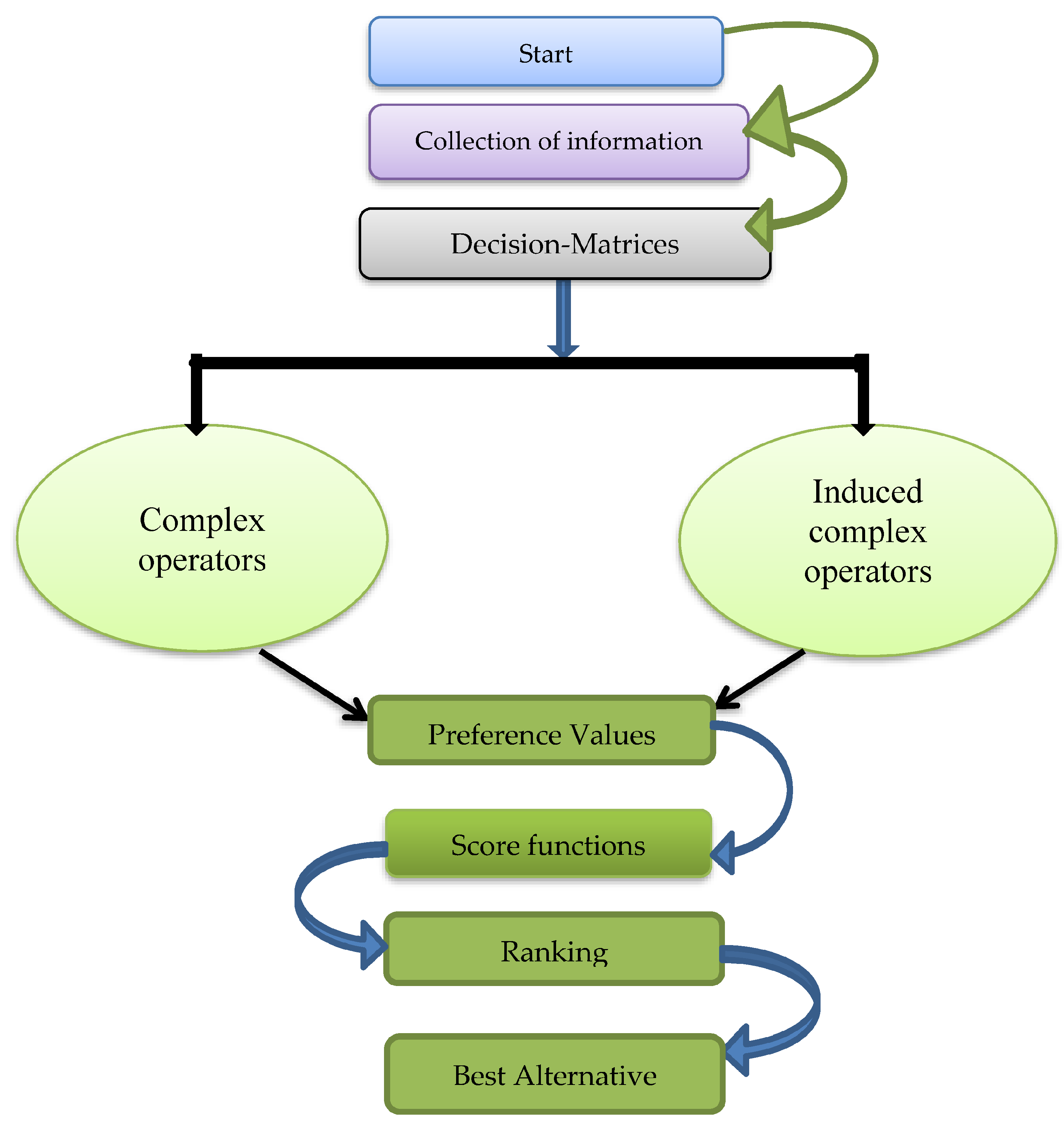
Let $\mathcal{H}=\left\{{\mathcal{H}}_1,{\mathcal{H}}_2,\dots ,{\mathcal{H}}_m\right\}$ be the set of m alternatives and $Ÿ=\left\{{Ÿ}_1,{Ÿ}_2,\dots ,{Ÿ}_n\right\}$ be the set of n criteria whose associated vector is $Є={\left({Є}_1,{Є}_2,\dots ,{Є}_n\right)}^T$ with restriction, such as $\left(1\le {Є}_j\le n\right)$ and ${\displaystyle \sum _{j=1}^n{Є}_j=1}$. ${\displaystyle \sum _{j=1}^n{\upsilon }_j=1}$. Let ${\rm E}=\left\{{{\rm E}}_1,{{\rm E}}_2,\dots ,{{\rm E}}_k\right\}$ be a group of k experts whose weighted vector is $\exists ={\left({\exists }_1,{\exists }_2,\dots ,{\exists }_k\right)}^T$ with settings, such as $\left(1\le {\exists }_j\le n\right)$ and ${\displaystyle \sum _{j=1}^k{\exists }_j}=1$. The main steps are as follows (Figure 1 for explanation): Step 1: Develop matrices based on the expertise of experts. Step 2: Make a single matrix out of all the separate matrices by combining them using the specified operators. Step 3: Again, compute all of the preference values using the specified techniques. Step 4: Calculate the scores using all preference values. Step 5: Choose the one with the highest score value.

6. Illustrative Example

Case study: In this section, we demonstrate an application of the proposed aggregation for China-reported cases of COVID-19. The first case was recorded in Wuhan, China, in December 2019, and the disease spread over the world in March 2020. At the start of 2020, the Chinese government imposed the biggest lockdown in human history, which caused millions of people to experience agony. Because multiple instances of COVID-19 were discovered in several hospitals in Pakistan in March 2020, Pakistan is regarded as the third Asian country with the highest number of coronavirus cases. Recently, certain mathematical models have been developed to clarify the coronavirus infection. These models mostly use real numbers and classical integer-order derivatives, which cannot capture fading memory. Therefore, it is difficult for the world at this time to comprehend and stop the spread of COVID-19. Therefore, the purpose of our paper is to formulate some new techniques, namely complex Pythagorean fuzzy weighted geometric (CPyFWG), complex Pythagorean fuzzy ordered weighted geometric (CPyFOWG), complex Pythagorean fuzzy hybrid geometric (CPyFHG), induced complex Pythagorean fuzzy ordered weighted geometric (I-CPyFOWG) and induced complex Pythagorean fuzzy hybrid geometric (I-CPyFHG) operator, to assess the spreading rate of COVID-19 and suggest particular hospitals for patients in specified geographic locations. So, the Pakistani government made the decision to limit patient access to a select group of hospitals in selected locations in an effort to contain the spread of COVID-19. For this, the government established a committee of four experts/doctors. $E_k\left(k=1,2,3,4\right)$ with a weighted vector $\exists ={\left(0.1,0.2,0.3,0.4\right)}^T$. There are four alternatives in the first section, ${\mathcal{H}}_m\left(m=1,2,3,4\right)$ have been considered for further selection. There are many factors that must be considered while choosing the more suitable location for a hospital, but here we have conceded the following five criteria for the hospital location, whose weight vector is $Є={\left(0.1,0.2,0.2,0.2,0.3\right)}^T$. ${Ÿ}_1$: Traffic Conditions, ${Ÿ}_2$: Building Structure, ${Ÿ}_3$: Facilities Around the Building, ${Ÿ}_4$: More Suitable for Patients, and ${Ÿ}_5$: Low Expenditure.

6.1. By Algebraic Operators

Here we construct 4 Tables, such as

Table 1. Decision of expert ${{\rm E}}_1$.

	${\mathit{Ÿ}}_{\mathbf{1}}$	${\mathit{Ÿ}}_{\mathbf{2}}$	${\mathit{Ÿ}}_{\mathbf{3}}$	${\mathit{Ÿ}}_{\mathbf{4}}$	${\mathit{Ÿ}}_{\mathbf{5}}$
${\mathcal{H}}_1$	$\left(\begin{array}{l}0.60e^{i2\pi \left(0.60\right)},\\ 0.70e^{i2\pi \left(0.50\right)}\end{array}\right)$	$\left(\begin{array}{l}0.70e^{i2\pi \left(0.50\right)},\\ 0.60e^{i2\pi \left(0.70\right)}\end{array}\right)$	$\left(\begin{array}{l}0.70e^{i2\pi \left(0.60\right)},\\ 0.60e^{i2\pi \left(0.70\right)}\end{array}\right)$	$\left(\begin{array}{l}0.70e^{i2\pi \left(0.50\right)},\\ 0.70e^{i2\pi \left(0.70\right)}\end{array}\right)$	$\left(\begin{array}{l}0.70e^{i2\pi \left(0.40\right)},\\ 0.60e^{i2\pi \left(0.70\right)}\end{array}\right)$
${\mathcal{H}}_2$	$\left(\begin{array}{l}0.50e^{i2\pi \left(0.40\right)},\\ 0.50e^{i2\pi \left(0.70\right)}\end{array}\right)$	$\left(\begin{array}{l}0.50e^{i2\pi \left(0.60\right)},\\ 0.60e^{i2\pi \left(0.70\right)}\end{array}\right)$	$\left(\begin{array}{l}0.70e^{i2\pi \left(0.40\right)},\\ 0.70e^{i2\pi \left(0.90\right)}\end{array}\right)$	$\left(\begin{array}{l}0.60e^{i2\pi \left(0.60\right)},\\ 0.70e^{i2\pi \left(0.70\right)}\end{array}\right)$	$\left(\begin{array}{l}0.60e^{i2\pi \left(0.80\right)},\\ 0.60e^{i2\pi \left(0.40\right)}\end{array}\right)$
${\mathcal{H}}_3$	$\left(\begin{array}{l}0.60e^{i2\pi \left(0.80\right)},\\ 0.60e^{i2\pi \left(0.40\right)}\end{array}\right)$	$\left(\begin{array}{l}0.60e^{i2\pi \left(0.60\right)},\\ 0.70e^{i2\pi \left(0.70\right)}\end{array}\right)$	$\left(\begin{array}{l}0.90e^{i2\pi \left(0.60\right)},\\ 0.40e^{i2\pi \left(0.70\right)}\end{array}\right)$	$\left(\begin{array}{l}0.50e^{i2\pi \left(0.60\right)},\\ 0.60e^{i2\pi \left(0.70\right)}\end{array}\right)$	$\left(\begin{array}{l}0.50e^{i2\pi \left(0.40\right)},\\ 0.50e^{i2\pi \left(0.70\right)}\end{array}\right)$
${\mathcal{H}}_4$	$\left(\begin{array}{l}0.70e^{i2\pi \left(0.40\right)},\\ 0.60e^{i2\pi \left(0.70\right)}\end{array}\right)$	$\left(\begin{array}{l}0.70e^{i2\pi \left(0.50\right)},\\ 0.70e^{i2\pi \left(0.70\right)}\end{array}\right)$	$\left(\begin{array}{l}0.50e^{i2\pi \left(0.70\right)},\\ 0.70e^{i2\pi \left(0.70\right)}\end{array}\right)$	$\left(\begin{array}{l}0.70e^{i2\pi \left(0.50\right)},\\ 0.60e^{i2\pi \left(0.70\right)}\end{array}\right)$	$\left(\begin{array}{l}0.60e^{i2\pi \left(0.60\right)},\\ 0.70e^{i2\pi \left(0.50\right)}\end{array}\right)$

,

Table 2. Decision of expert ${{\rm E}}_2$.

	${\mathit{Ÿ}}_{\mathbf{1}}$	${\mathit{Ÿ}}_{\mathbf{2}}$	${\mathit{Ÿ}}_{\mathbf{3}}$	${\mathit{Ÿ}}_{\mathbf{4}}$	${\mathit{Ÿ}}_{\mathbf{5}}$
${\mathcal{H}}_{\mathbf{1}}$	$\left(\begin{array}{l}0.70e^{i2\pi \left(0.60\right)},\\ 0.70e^{i2\pi \left(0.50\right)}\end{array}\right)$	$\left(\begin{array}{l}0.60e^{i2\pi \left(0.60\right)},\\ 0.70e^{i2\pi \left(0.70\right)}\end{array}\right)$	$\left(\begin{array}{l}0.90e^{i2\pi \left(0.60\right)},\\ 0.40e^{i2\pi \left(0.70\right)}\end{array}\right)$	$\left(\begin{array}{l}0.70e^{i2\pi \left(0.50\right)},\\ 0.60e^{i2\pi \left(0.70\right)}\end{array}\right)$	$\left(\begin{array}{l}0.50e^{i2\pi \left(0.40\right)},\\ 0.50e^{i2\pi \left(0.70\right)}\end{array}\right)$
${\mathcal{H}}_2$	$\left(\begin{array}{l}0.60e^{i2\pi \left(0.40\right)},\\ 0.50e^{i2\pi \left(0.70\right)}\end{array}\right)$	$\left(\begin{array}{l}0.50e^{i2\pi \left(0.60\right)},\\ 0.60e^{i2\pi \left(0.70\right)}\end{array}\right)$	$\left(\begin{array}{l}0.70e^{i2\pi \left(0.40\right)},\\ 0.70e^{i2\pi \left(0.90\right)}\end{array}\right)$	$\left(\begin{array}{l}0.60e^{i2\pi \left(0.60\right)},\\ 0.70e^{i2\pi \left(0.70\right)}\end{array}\right)$	$\left(\begin{array}{l}0.60e^{i2\pi \left(0.80\right)},\\ 0.60e^{i2\pi \left(0.40\right)}\end{array}\right)$
${\mathcal{H}}_3$	$\left(\begin{array}{l}0.60e^{i2\pi \left(0.80\right)},\\ 0.60e^{i2\pi \left(0.40\right)}\end{array}\right)$	$\left(\begin{array}{l}0.60e^{i2\pi \left(0.50\right)},\\ 0.60e^{i2\pi \left(0.70\right)}\end{array}\right)$	$\left(\begin{array}{l}0.70e^{i2\pi \left(0.60\right)},\\ 0.60e^{i2\pi \left(0.70\right)}\end{array}\right)$	$\left(\begin{array}{l}0.50e^{i2\pi \left(0.60\right)},\\ 0.60e^{i2\pi \left(0.70\right)}\end{array}\right)$	$\left(\begin{array}{l}0.70e^{i2\pi \left(0.40\right)},\\ 0.60e^{i2\pi \left(0.70\right)}\end{array}\right)$
${\mathcal{H}}_4$	$\left(\begin{array}{l}0.70e^{i2\pi \left(0.40\right)},\\ 0.60e^{i2\pi \left(0.70\right)}\end{array}\right)$	$\left(\begin{array}{l}0.70e^{i2\pi \left(0.50\right)},\\ 0.40e^{i2\pi \left(0.70\right)}\end{array}\right)$	$\left(\begin{array}{l}0.50e^{i2\pi \left(0.70\right)},\\ 0.70e^{i2\pi \left(0.70\right)}\end{array}\right)$	$\left(\begin{array}{l}0.70e^{i2\pi \left(0.50\right)},\\ 0.70e^{i2\pi \left(0.70\right)}\end{array}\right)$	$\left(\begin{array}{l}0.60e^{i2\pi \left(0.60\right)},\\ 0.70e^{i2\pi \left(0.50\right)}\end{array}\right)$

,

Table 3. Decision of expert ${{\rm E}}_3$.

	${\mathit{Ÿ}}_{\mathbf{1}}$	${\mathit{Ÿ}}_{\mathbf{2}}$	${\mathit{Ÿ}}_{\mathbf{3}}$	${\mathit{Ÿ}}_{\mathbf{4}}$	${\mathit{Ÿ}}_{\mathbf{5}}$
${\mathcal{H}}_1$	$\left(\begin{array}{l}0.70e^{i2\pi \left(0.60\right)},\\ 0.30e^{i2\pi \left(0.30\right)}\end{array}\right)$	$\left(\begin{array}{l}0.60e^{i2\pi \left(0.50\right)},\\ 0.40e^{i2\pi \left(0.40\right)}\end{array}\right)$	$\left(\begin{array}{l}0.50e^{i2\pi \left(0.40\right)},\\ 0.50e^{i2\pi \left(0.70\right)}\end{array}\right)$	$\left(\begin{array}{l}0.70e^{i2\pi \left(0.60\right)},\\ 0.30e^{i2\pi \left(0.30\right)}\end{array}\right)$	$\left(\begin{array}{l}0.70e^{i2\pi \left(0.40\right)},\\ 0.60e^{i2\pi \left(0.70\right)}\end{array}\right)$
${\mathcal{H}}_2$	$\left(\begin{array}{l}0.60e^{i2\pi \left(0.50\right)},\\ 0.40e^{i2\pi \left(0.40\right)}\end{array}\right)$	$\left(\begin{array}{l}0.50e^{i2\pi \left(0.60\right)},\\ 0.60e^{i2\pi \left(0.70\right)}\end{array}\right)$	$\left(\begin{array}{l}0.60e^{i2\pi \left(0.50\right)},\\ 0.40e^{i2\pi \left(0.40\right)}\end{array}\right)$	$\left(\begin{array}{l}0.60e^{i2\pi \left(0.60\right)},\\ 0.70e^{i2\pi \left(0.70\right)}\end{array}\right)$	$\left(\begin{array}{l}0.60e^{i2\pi \left(0.80\right)},\\ 0.60e^{i2\pi \left(0.40\right)}\end{array}\right)$
${\mathcal{H}}_3$	$\left(\begin{array}{l}0.60e^{i2\pi \left(0.80\right)},\\ 0.60e^{i2\pi \left(0.40\right)}\end{array}\right)$	$\left(\begin{array}{l}0.60e^{i2\pi \left(0.50\right)},\\ 0.60e^{i2\pi \left(0.70\right)}\end{array}\right)$	$\left(\begin{array}{l}0.70e^{i2\pi \left(0.60\right)},\\ 0.60e^{i2\pi \left(0.70\right)}\end{array}\right)$	$\left(\begin{array}{l}0.60e^{i2\pi \left(0.50\right)},\\ 0.40e^{i2\pi \left(0.40\right)}\end{array}\right)$	$\left(\begin{array}{l}0.60e^{i2\pi \left(0.50\right)},\\ 0.40e^{i2\pi \left(0.40\right)}\end{array}\right)$
${\mathcal{H}}_4$	$\left(\begin{array}{l}0.90e^{i2\pi \left(0.60\right)},\\ 0.40e^{i2\pi \left(0.70\right)}\end{array}\right)$	$\left(\begin{array}{l}0.70e^{i2\pi \left(0.60\right)},\\ 0.30e^{i2\pi \left(0.30\right)}\end{array}\right)$	$\left(\begin{array}{l}0.70e^{i2\pi \left(0.50\right)},\\ 0.70e^{i2\pi \left(0.70\right)}\end{array}\right)$	$\left(\begin{array}{l}0.50e^{i2\pi \left(0.70\right)},\\ 0.70e^{i2\pi \left(0.70\right)}\end{array}\right)$	$\left(\begin{array}{l}0.60e^{i2\pi \left(0.60\right)},\\ 0.30e^{i2\pi \left(0.50\right)}\end{array}\right)$

and

Table 4. Decision of expert ${{\rm E}}_4$.

	${\mathit{Ÿ}}_{\mathbf{1}}$	${\mathit{Ÿ}}_{\mathbf{2}}$	${\mathit{Ÿ}}_{\mathbf{3}}$	${\mathit{Ÿ}}_{\mathbf{4}}$	${\mathit{Ÿ}}_{\mathbf{5}}$
${\mathscr{H}}_1$	$\left(\begin{array}{l}0.60e^{i2\pi \left(0.60\right)},\\ 0.30e^{i2\pi \left(0.20\right)}\end{array}\right)$	$\left(\begin{array}{l}0.70e^{i2\pi \left(0.50\right)},\\ 0.40e^{i2\pi \left(0.40\right)}\end{array}\right)$	$\left(\begin{array}{l}0.80e^{i2\pi \left(0.60\right)},\\ 0.40e^{i2\pi \left(0.70\right)}\end{array}\right)$	$\left(\begin{array}{l}0.70e^{i2\pi \left(0.40\right)},\\ 0.60e^{i2\pi \left(0.70\right)}\end{array}\right)$	$\left(\begin{array}{l}0.70e^{i2\pi \left(0.60\right)},\\ 0.30e^{i2\pi \left(0.30\right)}\end{array}\right)$
${\mathscr{H}}_2$	$\left(\begin{array}{l}0.60e^{i2\pi \left(0.80\right)},\\ 0.60e^{i2\pi \left(0.40\right)}\end{array}\right)$	$\left(\begin{array}{l}0.50e^{i2\pi \left(0.60\right)},\\ 0.60e^{i2\pi \left(0.70\right)}\end{array}\right)$	$\left(\begin{array}{l}0.60e^{i2\pi \left(0.50\right)},\\ 0.40e^{i2\pi \left(0.40\right)}\end{array}\right)$	$\left(\begin{array}{l}0.60e^{i2\pi \left(0.60\right)},\\ 0.70e^{i2\pi \left(0.70\right)}\end{array}\right)$	$\left(\begin{array}{l}0.60e^{i2\pi \left(0.80\right)},\\ 0.60e^{i2\pi \left(0.40\right)}\end{array}\right)$
${\mathscr{H}}_3$	$\left(\begin{array}{l}0.60e^{i2\pi \left(0.50\right)},\\ 0.40e^{i2\pi \left(0.40\right)}\end{array}\right)$	$\left(\begin{array}{l}0.60e^{i2\pi \left(0.50\right)},\\ 0.60e^{i2\pi \left(0.70\right)}\end{array}\right)$	$\left(\begin{array}{l}0.70e^{i2\pi \left(0.50\right)},\\ 0.70e^{i2\pi \left(0.70\right)}\end{array}\right)$	$\left(\begin{array}{l}0.50e^{i2\pi \left(0.70\right)},\\ 0.70e^{i2\pi \left(0.70\right)}\end{array}\right)$	$\left(\begin{array}{l}0.60e^{i2\pi \left(0.50\right)},\\ 0.40e^{i2\pi \left(0.40\right)}\end{array}\right)$
${\mathscr{H}}_4$	$\left(\begin{array}{l}0.80e^{i2\pi \left(0.60\right)},\\ 0.40e^{i2\pi \left(0.70\right)}\end{array}\right)$	$\left(\begin{array}{l}0.70e^{i2\pi \left(0.40\right)},\\ 0.60e^{i2\pi \left(0.70\right)}\end{array}\right)$	$\left(\begin{array}{l}0.70e^{i2\pi \left(0.60\right)},\\ 0.60e^{i2\pi \left(0.70\right)}\end{array}\right)$	$\left(\begin{array}{l}0.60e^{i2\pi \left(0.50\right)},\\ 0.40e^{i2\pi \left(0.40\right)}\end{array}\right)$	$\left(\begin{array}{l}0.60e^{i2\pi \left(0.60\right)},\\ 0.30e^{i2\pi \left(0.50\right)}\end{array}\right)$

, for decision maker’s suggestion, and then combine all tables into a single table, such as

Table 5. Collective decision of all experts.

	${\mathit{Ÿ}}_{\mathbf{1}}$	${\mathit{Ÿ}}_{\mathbf{2}}$	${\mathit{Ÿ}}_{\mathbf{3}}$	${\mathit{Ÿ}}_{\mathbf{4}}$	${\mathit{Ÿ}}_{\mathbf{5}}$
${\mathcal{H}}_1$	$\left(\begin{array}{l}0.70e^{i2\pi \left(0.71\right)},\\ 0.55e^{i2\pi \left(0.68\right)}\end{array}\right)$	$\left(\begin{array}{l}0.64e^{i2\pi \left(0.51\right)},\\ 0.62e^{i2\pi \left(0.60\right)}\end{array}\right)$	$\left(\begin{array}{l}0.65e^{i2\pi \left(0.57\right)},\\ 0.56e^{i2\pi \left(0.66\right)}\end{array}\right)$	$\left(\begin{array}{l}0.66e^{i2\pi \left(0.54\right)},\\ 0.51e^{i2\pi \left(0.48\right)}\end{array}\right)$	$\left(\begin{array}{l}0.66e^{i2\pi \left(0.60\right)},\\ 0.52e^{i2\pi \left(0.45\right)}\end{array}\right)$
${\mathcal{H}}_2$	$\left(\begin{array}{l}0.59e^{i2\pi \left(0.54\right)},\\ 0.65e^{i2\pi \left(0.72\right)}\end{array}\right)$	$\left(\begin{array}{l}0.67e^{i2\pi \left(0.57\right)},\\ 0.56e^{i2\pi \left(0.45\right)}\end{array}\right)$	$\left(\begin{array}{l}0.52e^{i2\pi \left(0.66\right)},\\ 0.46e^{i2\pi \left(0.43\right)}\end{array}\right)$	$\left(\begin{array}{l}0.62e^{i2\pi \left(0.59\right)},\\ 0.50e^{i2\pi \left(0.48\right)}\end{array}\right)$	$\left(\begin{array}{l}0.62e^{i2\pi \left(0.56\right)},\\ 0.47e^{i2\pi \left(0.46\right)}\end{array}\right)$
${\mathcal{H}}_3$	$\left(\begin{array}{l}0.66e^{i2\pi \left(0.65\right)},\\ 0.63e^{i2\pi \left(0.53\right)}\end{array}\right)$	$\left(\begin{array}{l}0.60e^{i2\pi \left(0.50\right)},\\ 0.50e^{i2\pi \left(0.45\right)}\end{array}\right)$	$\left(\begin{array}{l}0.53e^{i2\pi \left(0.55\right)},\\ 0.51e^{i2\pi \left(0.41\right)}\end{array}\right)$	$\left(\begin{array}{l}0.63e^{i2\pi \left(0.50\right)},\\ 0.51e^{i2\pi \left(0.37\right)}\end{array}\right)$	$\left(\begin{array}{l}0.61e^{i2\pi \left(0.50\right)},\\ 0.50e^{i2\pi \left(0.43\right)}\end{array}\right)$
${\mathcal{H}}_4$	$\left(\begin{array}{l}0.68e^{i2\pi \left(0.58\right)},\\ 0.61e^{i2\pi \left(0.71\right)}\end{array}\right)$	$\left(\begin{array}{l}0.55e^{i2\pi \left(0.47\right)},\\ 0.49e^{i2\pi \left(0.44\right)}\end{array}\right)$	$\left(\begin{array}{l}0.65e^{i2\pi \left(0.52\right)},\\ 0.50e^{i2\pi \left(0.45\right)}\end{array}\right)$	$\left(\begin{array}{l}0.68e^{i2\pi \left(0.47\right)},\\ 0.61e^{i2\pi \left(0.50\right)}\end{array}\right)$	$\left(\begin{array}{l}0.62e^{i2\pi \left(0.61\right)},\\ 0.54e^{i2\pi \left(0.51\right)}\end{array}\right)$

:

• Step 1: The decision matrices can be constructed according to the ideas of experts as:

• Step 2: Combine all the individual matrices into one matrix using the CPyFWG operator, where $\exists ={\left(0.1,0.2,0.3,0.4\right)}^T$.

• Step 3: Again, using CPyFWG operator with $Є={\left(0.10,0.20,0.20,0.20,0.30\right)}^T$, and obtain

  $$r_1=\left(0.72e^{i2\pi \left(0.66\right)},0.49e^{i2\pi \left(0.52\right)}\right), r_2=\left(0.60e^{i2\pi \left(0.61\right)},0.54e^{i2\pi \left(0.37\right)}\right)$$

  $$r_3=\left(0.70e^{i2\pi \left(0.58\right)},0.43e^{i2\pi \left(0.51\right)}\right), r_4=\left(0.71e^{i2\pi \left(0.64\right)},0.50e^{i2\pi \left(0.62\right)}\right)$$

• Step 4: Computing the score functions as:

  $$Sc\left(r_1\right)={\left(0.72\right)}^2-{\left(0.49\right)}^2+\frac{1}{4{\pi }^2}\left({\left(0.66\right)}^2-{\left(0.52\right)}^2\right)=0.44$$

  $$Sc\left(r_2\right)={\left(0.60\right)}^2-{\left(0.54\right)}^2+\frac{1}{4{\pi }^2}\left({\left(0.61\right)}^2-{\left(0.37\right)}^2\right)=0.30$$

  $$Sc\left(r_3\right)={\left(0.70\right)}^2-{\left(0.43\right)}^2+\frac{1}{4{\pi }^2}\left({\left(0.58\right)}^2-{\left(0.51\right)}^2\right)=0.38$$

  $$Sc\left(r_4\right)={\left(0.71\right)}^2-{\left(0.50\right)}^2+\frac{1}{4{\pi }^2}\left({\left(0.68\right)}^2-{\left(0.60\right)}^2\right)=0.35$$

• Step 5: Thus, the best option is ${\mathcal{H}}_1$.

6.2. By Induced Aggregation Operators

Here we construct 4 Tables, such as

Table 6. Decision matrix under inducing variable of expert ${{\rm E}}_1$.

	${𝓗}_{\mathbf{1}}$	${𝓗}_{\mathbf{2}}$	${𝓗}_{\mathbf{3}}$	${𝓗}_{\mathbf{4}}$
${Ÿ}_1$	$〈0.9,\left(\begin{array}{l}0.60e^{i2\pi \left(0.60\right)},\\ 0.70e^{i2\pi \left(0.50\right)}\end{array}\right)〉$	$〈0.8,\left(\begin{array}{l}0.50e^{i2\pi \left(0.40\right)},\\ 0.50e^{i2\pi \left(0.70\right)}\end{array}\right)〉$	$〈0.6,\left(\begin{array}{l}0.60e^{i2\pi \left(0.80\right)},\\ 0.60e^{i2\pi \left(0.40\right)}\end{array}\right)〉$	$〈0.7,\left(\begin{array}{l}0.70e^{i2\pi \left(0.40\right)},\\ 0.60e^{i2\pi \left(0.70\right)}\end{array}\right)〉$
${Ÿ}_2$	$〈0.7,\left(\begin{array}{l}0.70e^{i2\pi \left(0.50\right)},\\ 0.60e^{i2\pi \left(0.70\right)}\end{array}\right)〉$	$〈0.6,\left(\begin{array}{l}0.50e^{i2\pi \left(0.60\right)},\\ 0.60e^{i2\pi \left(0.70\right)}\end{array}\right)〉$	$〈0.7,\left(\begin{array}{l}0.60e^{i2\pi \left(0.60\right)},\\ 0.70e^{i2\pi \left(0.70\right)}\end{array}\right)〉$	$〈0.9,\left(\begin{array}{l}0.70e^{i2\pi \left(0.50\right)},\\ 0.70e^{i2\pi \left(0.70\right)}\end{array}\right)〉$
${Ÿ}_3$	$〈0.6,\left(\begin{array}{l}0.70e^{i2\pi \left(0.60\right)},\\ 0.60e^{i2\pi \left(0.70\right)}\end{array}\right)〉$	$〈0.7,\left(\begin{array}{l}0.70e^{i2\pi \left(0.40\right)},\\ 0.70e^{i2\pi \left(0.90\right)}\end{array}\right)〉$	$〈0.5,\left(\begin{array}{l}0.90e^{i2\pi \left(0.60\right)},\\ 0.40e^{i2\pi \left(0.70\right)}\end{array}\right)〉$	$〈0.5,\left(\begin{array}{l}0.50e^{i2\pi \left(0.70\right)},\\ 0.70e^{i2\pi \left(0.70\right)}\end{array}\right)〉$
${Ÿ}_4$	$〈0.8,\left(\begin{array}{l}0.70e^{i2\pi \left(0.50\right)},\\ 0.70e^{i2\pi \left(0.70\right)}\end{array}\right)〉$	$〈0.4,\left(\begin{array}{l}0.60e^{i2\pi \left(0.60\right)},\\ 0.70e^{i2\pi \left(0.70\right)}\end{array}\right)〉$	$〈0.8,\left(\begin{array}{l}0.50e^{i2\pi \left(0.60\right)},\\ 0.60e^{i2\pi \left(0.70\right)}\end{array}\right)〉$	$〈0.5,\left(\begin{array}{l}0.70e^{i2\pi \left(0.50\right)},\\ 0.60e^{i2\pi \left(0.70\right)}\end{array}\right)〉$
${Ÿ}_5$	$〈0.6,\left(\begin{array}{l}0.70e^{i2\pi \left(0.40\right)},\\ 0.60e^{i2\pi \left(0.70\right)}\end{array}\right)〉$	$〈0.8,\left(\begin{array}{l}0.60e^{i2\pi \left(0.80\right)},\\ 0.60e^{i2\pi \left(0.40\right)}\end{array}\right)〉$	$〈0.4,\left(\begin{array}{l}0.50e^{i2\pi \left(0.40\right)},\\ 0.50e^{i2\pi \left(0.70\right)}\end{array}\right)〉$	$〈0.3,\left(\begin{array}{l}0.60e^{i2\pi \left(0.60\right)},\\ 0.70e^{i2\pi \left(0.50\right)}\end{array}\right)〉$

,

Table 7. Decision matrix under inducing variable of expert ${{\rm E}}_2$.

	${𝓗}_1$	${𝓗}_2$	${𝓗}_3$	${𝓗}_4$
${Ÿ}_1$	$〈0.8,\left(\begin{array}{l}0.70e^{i2\pi \left(0.60\right)},\\ 0.70e^{i2\pi \left(0.50\right)}\end{array}\right)〉$	$〈0.9,\left(\begin{array}{l}0.60e^{i2\pi \left(0.40\right)},\\ 0.50e^{i2\pi \left(0.70\right)}\end{array}\right)〉$	$〈0.3,\left(\begin{array}{l}0.60e^{i2\pi \left(0.80\right)},\\ 0.60e^{i2\pi \left(0.40\right)}\end{array}\right)〉$	$〈0.8,\left(\begin{array}{l}0.70e^{i2\pi \left(0.40\right)},\\ 0.60e^{i2\pi \left(0.70\right)}\end{array}\right)〉$
${Ÿ}_2$	$〈0.8,\left(\begin{array}{l}0.60e^{i2\pi \left(0.60\right)},\\ 0.70e^{i2\pi \left(0.70\right)}\end{array}\right)〉$	$〈0.7,\left(\begin{array}{l}0.50e^{i2\pi \left(0.60\right)},\\ 0.60e^{i2\pi \left(0.70\right)}\end{array}\right)〉$	$〈0.5,\left(\begin{array}{l}0.60e^{i2\pi \left(0.50\right)},\\ 0.60e^{i2\pi \left(0.70\right)}\end{array}\right)〉$	$〈0.6,\left(\begin{array}{l}0.70e^{i2\pi \left(0.50\right)},\\ 0.40e^{i2\pi \left(0.70\right)}\end{array}\right)〉$
${Ÿ}_3$	$〈0.4,\left(\begin{array}{l}0.90e^{i2\pi \left(0.60\right)},\\ 0.40e^{i2\pi \left(0.70\right)}\end{array}\right)〉$	$〈0.5,\left(\begin{array}{l}0.70e^{i2\pi \left(0.40\right)},\\ 0.70e^{i2\pi \left(0.90\right)}\end{array}\right)〉$	$〈0.7,\left(\begin{array}{l}0.70e^{i2\pi \left(0.60\right)},\\ 0.60e^{i2\pi \left(0.70\right)}\end{array}\right)〉$	$〈0.4,\left(\begin{array}{l}0.50e^{i2\pi \left(0.70\right)},\\ 0.70e^{i2\pi \left(0.70\right)}\end{array}\right)〉$
${Ÿ}_4$	$〈0.4,\left(\begin{array}{l}0.70e^{i2\pi \left(0.50\right)},\\ 0.60e^{i2\pi \left(0.70\right)}\end{array}\right)〉$	$〈0.3,\left(\begin{array}{l}0.60e^{i2\pi \left(0.60\right)},\\ 0.70e^{i2\pi \left(0.70\right)}\end{array}\right)〉$	$〈0.7,\left(\begin{array}{l}0.50e^{i2\pi \left(0.60\right)},\\ 0.60e^{i2\pi \left(0.70\right)}\end{array}\right)〉$	$〈0.4,\left(\begin{array}{l}0.70e^{i2\pi \left(0.50\right)},\\ 0.70e^{i2\pi \left(0.70\right)}\end{array}\right)〉$
${Ÿ}_5$	$〈0.2,\left(\begin{array}{l}0.50e^{i2\pi \left(0.40\right)},\\ 0.50e^{i2\pi \left(0.70\right)}\end{array}\right)〉$	$〈0.3,\left(\begin{array}{l}0.60e^{i2\pi \left(0.80\right)},\\ 0.60e^{i2\pi \left(0.40\right)}\end{array}\right)〉$	$〈0.9,\left(\begin{array}{l}0.70e^{i2\pi \left(0.40\right)},\\ 0.60e^{i2\pi \left(0.70\right)}\end{array}\right)〉$	$〈0.2,\left(\begin{array}{l}0.60e^{i2\pi \left(0.60\right)},\\ 0.70e^{i2\pi \left(0.50\right)}\end{array}\right)〉$

,

Table 8. Decision matrix under inducing variable of expert ${{\rm E}}_3$.

	${𝓗}_1$	${𝓗}_2$	${𝓗}_3$	${𝓗}_4$
${Ÿ}_1$	$〈0.7,\left(\begin{array}{l}0.70e^{i2\pi \left(0.60\right)},\\ 0.30e^{i2\pi \left(0.30\right)}\end{array}\right)〉$	$〈0.6,\left(\begin{array}{l}0.60e^{i2\pi \left(0.50\right)},\\ 0.40e^{i2\pi \left(0.40\right)}\end{array}\right)〉$	$〈0.5,\left(\begin{array}{l}0.60e^{i2\pi \left(0.80\right)},\\ 0.60e^{i2\pi \left(0.40\right)}\end{array}\right)〉$	$〈0.9,\left(\begin{array}{l}0.90e^{i2\pi \left(0.60\right)},\\ 0.40e^{i2\pi \left(0.70\right)}\end{array}\right)〉$
${Ÿ}_2$	$〈0.9,\left(\begin{array}{l}0.60e^{i2\pi \left(0.50\right)},\\ 0.40e^{i2\pi \left(0.40\right)}\end{array}\right)〉$	$〈0.8,\left(\begin{array}{l}0.50e^{i2\pi \left(0.60\right)},\\ 0.60e^{i2\pi \left(0.70\right)}\end{array}\right)〉$	$〈0.6,\left(\begin{array}{l}0.60e^{i2\pi \left(0.50\right)},\\ 0.60e^{i2\pi \left(0.70\right)}\end{array}\right)〉$	$〈0.7,\left(\begin{array}{l}0.70e^{i2\pi \left(0.60\right)},\\ 0.30e^{i2\pi \left(0.30\right)}\end{array}\right)〉$
${Ÿ}_3$	$〈0.7,\left(\begin{array}{l}0.50e^{i2\pi \left(0.40\right)},\\ 0.50e^{i2\pi \left(0.70\right)}\end{array}\right)〉$	$〈0.4,\left(\begin{array}{l}0.60e^{i2\pi \left(0.50\right)},\\ 0.40e^{i2\pi \left(0.40\right)}\end{array}\right)〉$	$〈0.4,\left(\begin{array}{l}0.70e^{i2\pi \left(0.60\right)},\\ 0.60e^{i2\pi \left(0.70\right)}\end{array}\right)〉$	$〈0.3,\left(\begin{array}{l}0.70e^{i2\pi \left(0.50\right)},\\ 0.70e^{i2\pi \left(0.70\right)}\end{array}\right)〉$
${Ÿ}_4$	$〈0.5,\left(\begin{array}{l}0.70e^{i2\pi \left(0.60\right)},\\ 0.30e^{i2\pi \left(0.30\right)}\end{array}\right)〉$	$〈0.7,\left(\begin{array}{l}0.60e^{i2\pi \left(0.60\right)},\\ 0.70e^{i2\pi \left(0.70\right)}\end{array}\right)〉$	$〈0.5,\left(\begin{array}{l}0.60e^{i2\pi \left(0.50\right)},\\ 0.40e^{i2\pi \left(0.40\right)}\end{array}\right)〉$	$〈0.3,\left(\begin{array}{l}0.50e^{i2\pi \left(0.70\right)},\\ 0.70e^{i2\pi \left(0.70\right)}\end{array}\right)〉$
${Ÿ}_5$	$〈0.4,\left(\begin{array}{l}0.70e^{i2\pi \left(0.40\right)},\\ 0.60e^{i2\pi \left(0.70\right)}\end{array}\right)〉$	$〈0.5,\left(\begin{array}{l}0.60e^{i2\pi \left(0.80\right)},\\ 0.60e^{i2\pi \left(0.40\right)}\end{array}\right)〉$	$〈0.3,\left(\begin{array}{l}0.60e^{i2\pi \left(0.50\right)},\\ 0.40e^{i2\pi \left(0.40\right)}\end{array}\right)〉$	$〈0.5,\left(\begin{array}{l}0.60e^{i2\pi \left(0.60\right)},\\ 0.30e^{i2\pi \left(0.50\right)}\end{array}\right)〉$

and

Table 9. Decision matrix under inducing variable of expert ${{\rm E}}_4$.

	${𝓗}_1$	${𝓗}_2$	${𝓗}_3$	${𝓗}_4$
${Ÿ}_1$	$〈0.5,\left(\begin{array}{l}0.60e^{i2\pi \left(0.60\right)},\\ 0.30e^{i2\pi \left(0.20\right)}\end{array}\right)〉$	$〈0.4,\left(\begin{array}{l}0.60e^{i2\pi \left(0.80\right)},\\ 0.60e^{i2\pi \left(0.40\right)}\end{array}\right)〉$	$〈0.8,\left(\begin{array}{l}0.60e^{i2\pi \left(0.50\right)},\\ 0.40e^{i2\pi \left(0.40\right)}\end{array}\right)〉$	$〈0.6,\left(\begin{array}{l}0.80e^{i2\pi \left(0.60\right)},\\ 0.40e^{i2\pi \left(0.70\right)}\end{array}\right)〉$
${Ÿ}_2$	$〈0.4,\left(\begin{array}{l}0.70e^{i2\pi \left(0.50\right)},\\ 0.40e^{i2\pi \left(0.40\right)}\end{array}\right)〉$	$〈0.3,\left(\begin{array}{l}0.50e^{i2\pi \left(0.60\right)},\\ 0.60e^{i2\pi \left(0.70\right)}\end{array}\right)〉$	$〈0.2,\left(\begin{array}{l}0.60e^{i2\pi \left(0.50\right)},\\ 0.60e^{i2\pi \left(0.70\right)}\end{array}\right)〉$	$〈0.3,\left(\begin{array}{l}0.70e^{i2\pi \left(0.40\right)},\\ 0.60e^{i2\pi \left(0.70\right)}\end{array}\right)〉$
${Ÿ}_3$	$〈0.5,\left(\begin{array}{l}0.80e^{i2\pi \left(0.60\right)},\\ 0.40e^{i2\pi \left(0.70\right)}\end{array}\right)〉$	$〈0.9,\left(\begin{array}{l}0.60e^{i2\pi \left(0.50\right)},\\ 0.40e^{i2\pi \left(0.40\right)}\end{array}\right)〉$	$\left(0.8,\left(\begin{array}{l}0.70e^{i2\pi \left(0.50\right)},\\ 0.70e^{i2\pi \left(0.70\right)}\end{array}\right)\right)$	$〈0.9,\left(\begin{array}{l}0.70e^{i2\pi \left(0.60\right)},\\ 0.60e^{i2\pi \left(0.70\right)}\end{array}\right)〉$
${Ÿ}_4$	$〈0.3,\left(\begin{array}{l}0.70e^{i2\pi \left(0.40\right)},\\ 0.60e^{i2\pi \left(0.70\right)}\end{array}\right)〉$	$〈0.6,\left(\begin{array}{l}0.60e^{i2\pi \left(0.60\right)},\\ 0.70e^{i2\pi \left(0.70\right)}\end{array}\right)〉$	$〈0.9,\left(\begin{array}{l}0.50e^{i2\pi \left(0.70\right)},\\ 0.70e^{i2\pi \left(0.70\right)}\end{array}\right)〉$	$〈0.7,\left(\begin{array}{l}0.60e^{i2\pi \left(0.50\right)},\\ 0.40e^{i2\pi \left(0.40\right)}\end{array}\right)〉$
${Ÿ}_5$	$〈0.7,\left(\begin{array}{l}0.70e^{i2\pi \left(0.60\right)},\\ 0.30e^{i2\pi \left(0.30\right)}\end{array}\right)〉$	$〈0.4,\left(\begin{array}{l}0.60e^{i2\pi \left(0.80\right)},\\ 0.60e^{i2\pi \left(0.40\right)}\end{array}\right)〉$	$〈0.8,\left(\begin{array}{l}0.60e^{i2\pi \left(0.50\right)},\\ 0.40e^{i2\pi \left(0.40\right)}\end{array}\right)〉$	$〈0.4,\left(\begin{array}{l}0.60e^{i2\pi \left(0.60\right)},\\ 0.30e^{i2\pi \left(0.50\right)}\end{array}\right)〉$

, for decision maker’s suggestion, and then combine all tables into a single table, such as

Table 10. Collective decision matrix under inducing variables.

	${𝓗}_1$	${𝓗}_2$	${𝓗}_3$	${𝓗}_4$
${Ÿ}_1$	$\left(\begin{array}{l}0.66e^{i2\pi \left(0.67\right)},\\ 0.48e^{i2\pi \left(0.53\right)}\end{array}\right)$	$\left(\begin{array}{l}0.62e^{i2\pi \left(0.58\right)},\\ 0.50e^{i2\pi \left(0.59\right)}\end{array}\right)$	$\left(\begin{array}{l}0.66e^{i2\pi \left(0.65\right)},\\ 0.65e^{i2\pi \left(0.43\right)}\end{array}\right)$	$\left(\begin{array}{l}0.72e^{i2\pi \left(0.61\right)},\\ 0.64e^{i2\pi \left(0.54\right)}\end{array}\right)$
${Ÿ}_2$	$\left(\begin{array}{l}0.64e^{i2\pi \left(0.59\right)},\\ 0.56e^{i2\pi \left(0.50\right)}\end{array}\right)$	$\left(\begin{array}{l}0.67e^{i2\pi \left(0.67\right)},\\ 0.53e^{i2\pi \left(0.50\right)}\end{array}\right)$	$\left(\begin{array}{l}0.70e^{i2\pi \left(0.60\right)},\\ 0.60e^{i2\pi \left(0.46\right)}\end{array}\right)$	$\left(\begin{array}{l}0.75e^{i2\pi \left(0.67\right)},\\ 0.47e^{i2\pi \left(0.48\right)}\end{array}\right)$
${Ÿ}_3$	$\left(\begin{array}{l}0.65e^{i2\pi \left(0.57\right)},\\ 0.56e^{i2\pi \left(0.46\right)}\end{array}\right)$	$\left(\begin{array}{l}0.72e^{i2\pi \left(0.66\right)},\\ 0.66e^{i2\pi \left(0.53\right)}\end{array}\right)$	$\left(\begin{array}{l}0.63e^{i2\pi \left(0.65\right)},\\ 0.58e^{i2\pi \left(0.51\right)}\end{array}\right)$	$\left(\begin{array}{l}0.65e^{i2\pi \left(0.62\right)},\\ 0.50e^{i2\pi \left(0.55\right)}\end{array}\right)$
${Ÿ}_4$	$\left(\begin{array}{l}0.70e^{i2\pi \left(0.74\right)},\\ 0.61e^{i2\pi \left(0.38\right)}\end{array}\right)$	$\left(\begin{array}{l}0.62e^{i2\pi \left(0.69\right)},\\ 0.50e^{i2\pi \left(0.48\right)}\end{array}\right)$	$\left(\begin{array}{l}0.63e^{i2\pi \left(0.70\right)},\\ 0.51e^{i2\pi \left(0.47\right)}\end{array}\right)$	$\left(\begin{array}{l}0.70e^{i2\pi \left(0.77\right)},\\ 0.71e^{i2\pi \left(0.60\right)}\end{array}\right)$
${Ÿ}_5$	$\left(\begin{array}{l}0.65e^{i2\pi \left(0.70\right)},\\ 0.51e^{i2\pi \left(0.55\right)}\end{array}\right)$	$\left(\begin{array}{l}0.72e^{i2\pi \left(0.59\right)},\\ 0.67e^{i2\pi \left(0.46\right)}\end{array}\right)$	$\left(\begin{array}{l}0.67e^{i2\pi \left(0.70\right)},\\ 0.60e^{i2\pi \left(0.60\right)}\end{array}\right)$	$\left(\begin{array}{l}0.67e^{i2\pi \left(0.71\right)},\\ 0.60e^{i2\pi \left(0.41\right)}\end{array}\right)$

:

• Step 1: Construct the following same matrices based on experts’ ideas:

• Step 2: Combine all the individual matrices into a single matrix using 1-CPFOWG aggregation operator, where $\psi ={\left(0.4,0.3,0.2,0.1\right)}^T$.

• Step 3: Again, using I-CPyFOWG operator, where $Є={\left(0.1,0.2,0.2,0.2,0.3\right)}^T$, and obtain all the preference values as below:

  $$r_1=\left(0.68e^{i2\pi \left(0.66\right)},0.58e^{i2\pi \left(0.52\right)}\right), r_2=\left(0.70e^{i2\pi \left(0.68\right)},0.63e^{i2\pi \left(0.55\right)}\right)$$

  $$r_3=\left(0.68e^{i2\pi \left(0.54\right)},0.67e^{i2\pi \left(0.59\right)}\right), r_4=\left(0.61e^{i2\pi \left(0.46\right)},0.68e^{i2\pi \left(0.60\right)}\right)$$

• Step 4: Again, computing the score functions as below.

  $$Sc\left(r_1\right)={\left(0.68\right)}^2-{\left(0.58\right)}^2+\frac{1}{4{\pi }^2}\left({\left(0.66\right)}^2-{\left(0.52\right)}^2\right)=0.29$$

  $$Sc\left(r_2\right)={\left(0.70\right)}^2-{\left(0.63\right)}^2+\frac{1}{4{\pi }^2}\left({\left(0.68\right)}^2-{\left(0.55\right)}^2\right)=0.25$$

  $$Sc\left(r_3\right)={\left(0.68\right)}^2-{\left(0.67\right)}^2+\frac{1}{4{\pi }^2}\left({\left(0.54\right)}^2-{\left(0.59\right)}^2\right)=0.27$$

  $$Sc\left(r_4\right)={\left(0.61\right)}^2-{\left(0.68\right)}^2+\frac{1}{4{\pi }^2}\left({\left(0.46\right)}^2-{\left(0.60\right)}^2\right)=0.26$$

• Step 5: Thus, the best option is ${\mathcal{H}}_1$.

Now, we construct

Table 11. Score of all methods.

Methods	Scores	Ranking
CPyFWG	$Sc\left(r_1\right)\succ Sc\left(r_3\right)\succ Sc\left(r_4\right)\succ Sc\left(r_2\right)$	${\mathcal{H}}_1\succ {\mathcal{H}}_3\succ {\mathcal{H}}_4\succ {\mathcal{H}}_2$
CPyFOWG	$Sc\left(r_1\right)\succ Sc\left(r_3\right)\succ Sc\left(r_4\right)\succ Sc\left(r_2\right)$	${\mathcal{H}}_1\succ {\mathcal{H}}_3\succ {\mathcal{H}}_4\succ {\mathcal{H}}_2$
CPyFHG	$Sc\left(r_1\right)\succ Sc\left(r_3\right)\succ Sc\left(r_4\right)\succ Sc\left(r_2\right)$	${\mathcal{H}}_1\succ {\mathcal{H}}_3\succ {\mathcal{H}}_4\succ {\mathcal{H}}_2$
I-CPyFOWG	$Sc\left(r_1\right)\succ Sc\left(r_3\right)\succ Sc\left(r_4\right)\succ Sc\left(r_2\right)$	${\mathcal{H}}_1\succ {\mathcal{H}}_3\succ {\mathcal{H}}_4\succ {\mathcal{H}}_2$
I-CPyFHG	$Sc\left(r_1\right)\succ Sc\left(r_3\right)\succ Sc\left(r_4\right)\succ Sc\left(r_2\right)$	${\mathcal{H}}_1\succ {\mathcal{H}}_3\succ {\mathcal{H}}_4\succ {\mathcal{H}}_2$

: for all aggregation operators and their score function:

7. Comparative Analysis

The Complex Pythagorean fuzzy set is a refinement of earlier studies, such as fuzzy sets, intuitionistic fuzzy sets, Pythagorean fuzzy sets, Fermatean fuzzy sets, complex fuzzy sets, and complex intuitionistic fuzzy sets, taking into account significantly more details about an object when processing it and managing two-dimensional data as a single set. For example, fuzzy sets have only one element membership grade under a real valued function, and there is no concept of non-membership function. Intuitionistic fuzzy sets, Pythagorean fuzzy sets, and Fermatean fuzzy sets have both degrees, such as membership grade and non-membership grade under real valued functions under conditions such as their sum, square sum, and cubic sum, which are equal to or less than one, respectively. On the other hand, complex fuzzy sets have only membership grade under complex valued function. For complex intuitionistic fuzzy sets and complex Pythagorean fuzzy sets, 55 have the membership grade and non-membership grade under complex-valued functions. Thus, compared to their earlier and preceding studies, the novel proposed model is more flexible and effective.

8. Sensitivity Analysis

Complex Pythagorean fuzzy set is one of the successful extensions of complex fuzzy set and complex intuitionistic fuzzy set. Complex Pythagorean fuzzy set not only applicable to complex Pythagorean fuzzy data, as it may be applicable to intuitionistic fuzzy data and Pythagorean fuzzy data by considering the phase terms to zero. Therefore, we can say that the proposed model is more elastic and flexible compared to the previous model, such as intuitionistic fuzzy set and Pythagorean fuzzy set. In the following

Table 12. Stated the sensitivity analysis.

Model	Uncertainty	Falsity	Hesitation	Periodicity	2-D Information	Square in Power
FSs	✓	✕	✕	✕	✕	✕
IFSs	✓	✓	✓	✕	✕	✕
PyFSs	✓	✓	✓	✕	✕	✕
FeFSs	✓	✓	✓	✕	✕	✕
CFSs	✓	✕	✕	✓	✓	✕
CIFSs	✓	✓	✓	✓	✓	✕
CPyFSs	✓	✓	✓	✓	✓	✓

: we show that our proposed model is more flexible as compared to their existing models.

9. Conclusions

In this research, we have improved several novel geometric aggregation operators based on complex Pythagorean fuzzy numbers, namely CPyFWG operator, CPyFOWG operator, CPyFHG operator, I-CPyFOWG operator, and I-CPyFHG operator, along with some examples and their structure properties, such as monotonicity, boundedness, and idempotency. To demonstrate the usefulness and efficiency of the proposed approach, an example involving the selection of a hospital location that is most appropriate is taken into consideration. A new comparison of the methodology and sensitivity analyses was also provided. Finally, a comparison and sensitivity analysis of the innovative model is given, demonstrating the potency of the strategy being offered.

Furthermore, this research can be expanded to complex Logarithmic aggregation operators, complex Dombi aggregation operators, complex symmetric aggregation operators, complex linguistic terms, complex power aggregation operators, complex Hamacher operators, complex Einstein approaches, complex confidence level, complex interval-valued aggregation operators, complex Dombi interval aggregation operators, complex Einstein interval-valued aggregation operators, and complex Hamacher interval-valued aggregation operators, etc.

References

1. Zadeh, L.A. Fuzzy sets. Inf. Control. 1965, 8, 338–353. [Google Scholar] [CrossRef] [Green Version]
2. Atanassov, K.T. Intuitionistic fuzzy sets. Fuzzy Sets Syst. 1986, 20, 87–96. [Google Scholar] [CrossRef]
3. Yager, R.R. Pythagorean Membership Grades in Multicriteria Decision Making. IEEE Trans. Fuzzy Syst. 2013, 22, 958–965. [Google Scholar] [CrossRef]
4. Senapati, T.; Yager, R.R. Fermatean fuzzy sets. J. Ambient. Intell. Humaniz. Comput. 2019, 11, 663–674. [Google Scholar] [CrossRef]
5. Xu, Z. Intuitionistic Fuzzy Aggregation Operators. IEEE Trans. Fuzzy Syst. 2007, 15, 1179–1187. [Google Scholar] [CrossRef]
6. Xu, Z.; Yager, R.R. Some geometric aggregation operators based on intuitionistic fuzzy sets. Int. J. Gen. Syst. 2006, 35, 417–433. [Google Scholar] [CrossRef]
7. Wang, W.; Liu, X. Intuitionistic fuzzy geometric aggregation operators based on einstein operations. Int. J. Intell. Syst. 2011, 26, 1049–1075. [Google Scholar] [CrossRef]
8. Wang, W.; Liu, X. Intuitionistic Fuzzy Information Aggregation Using Einstein Operations. IEEE Trans. Fuzzy Syst. 2012, 20, 923–938. [Google Scholar] [CrossRef]
9. Rahman, K.; Abdullah, S.; Jamil, M.; Khan, M.Y. Some Generalized Intuitionistic Fuzzy Einstein Hybrid Aggregation Operators and Their Application to Multiple Attribute Group Decision Making. Int. J. Fuzzy Syst. 2018, 20, 1567–1575. [Google Scholar] [CrossRef]
10. Rahman, K. Some new logarithmic aggregation operators and their application to group decision making problem based on t-norm and t-conorm. Soft Comput. 2022, 26, 2751–2772. [Google Scholar] [CrossRef]
11. Ahmmad, J.; Mahmood, T.; Mehmood, N.; Urawong, K.; Chinram, R. Intuitionistic Fuzzy Rough Aczel-Alsina Average Aggregation Operators and Their Applications in Medical Diagnoses. Symmetry 2022, 14, 2537. [Google Scholar] [CrossRef]
12. Rahman, K.; Khan, M.S.A.; Ullah, M.; Fahmi, A. Multiple Attribute Group Decision Making for Plant Location Selection with Pythagorean Fuzzy Weighted Geometric Aggregation Operator. Nucleus 2017, 54, 66–74. [Google Scholar]
13. Rahman, K.; Abdullah, S.; Hussain, F.; Khan, M.S.A.; Shakeel, M. Pythagorean Fuzzy Ordered Weighted Geometric Aggregation Operator and Their Application to Multiple Attribute Group Decision Making. J. Appl. Environ. Biol. Sci. 2017, 7, 67–83. [Google Scholar]
14. Rahman, K.; Abdullah, S.; Khan, M.S.A.; Shakeel, M. Pythagorean fuzzy hybrid geometric operator and their application to multiple attribute decision making. Int. J. Comput. Sci. Inf. Secur. 2016, 14, 837–854. [Google Scholar]
15. Rahman, K.; Khan, M.S.A.; Ullah, M. New Approaches to Pythagorean Fuzzy Averaging Aggregation Operators. Math. Lett. 2017, 3, 29. [Google Scholar] [CrossRef]
16. Garg, H. A New Generalized Pythagorean Fuzzy Information Aggregation Using Einstein Operations and Its Application to Decision Making. Int. J. Intell. Syst. 2016, 31, 886–920. [Google Scholar] [CrossRef]
17. Garg, H. Generalized Pythagorean fuzzy geometric aggregation operators using Einstein t-norm and t-conorm for multicriteria decision-making process. Int. J. Intell. Syst. 2017, 32, 597–630. [Google Scholar] [CrossRef]
18. Zulqarnain, R.M.; Siddique, I.; Ahmad, S.; Iampan, A.; Jovanov, G.; Vranješ, D.; Vasiljević, J. Pythagorean Fuzzy Soft Einstein Ordered Weighted Average Operator in Sustainable Supplier Selection Problem. Math. Probl. Eng. 2021, 2021, 1–16. [Google Scholar] [CrossRef]
19. Zulqarnain, R.M.; Siddique, I.; Ei-Morsy, S. Einstein-Ordered Weighted Geometric Operator for Pythagorean Fuzzy Soft Set with Its Application to Solve MAGDM Problem. Math. Probl. Eng. 2022, 2022, 1–14. [Google Scholar] [CrossRef]
20. Zulqarnain, R.M.; Siddique, I.; Jarad, F.; Hamed, Y.S.; Abualnaja, K.M.; Iampan, A. Einstein Aggregation Operators for Pythagorean Fuzzy Soft Sets with Their Application in Multiattribute Group Decision-Making. J. Funct. Spaces 2022, 2022, 1–21. [Google Scholar] [CrossRef]
21. Zulqarnain, R.M.; Dayan, F. Selection of Best Alternative for An Automotive Company by Intuitionistic Fuzzy TOPSIS Method. Int. J. Sci. Technol. Res. 2017, 6, 126–132. [Google Scholar]
22. Ramot, D.; Milo, R.; Friedman, M.; Kandel, A. Complex fuzzy sets. IEEE Trans Fuzzy Syst. 2002, 10, 171–186. [Google Scholar] [CrossRef]
23. Alkouri, A.S.; Salleh, A.R. Complex intuitionistic fuzzy sets. AIP Conf. Proc. 2012, 1482, 464–470. [Google Scholar] [CrossRef]
24. Ma, J.; Zhang, G.; Lu, J. A Method for Multiple Periodic Factor Prediction Problems Using Complex Fuzzy Sets. IEEE Trans. Fuzzy Syst. 2011, 20, 32–45. [Google Scholar] [CrossRef]
25. Dick, S.; Yager, R.R.; Yazdanbakhsh, O. On Pythagorean and Complex Fuzzy Set Operations. IEEE Trans. Fuzzy Syst. 2015, 24, 1009–1021. [Google Scholar] [CrossRef]
26. Liu, L.; Zhang, X. Comment on Pythagorean and Complex Fuzzy Set Operations. IEEE Trans. Fuzzy Syst. 2018, 26, 3902–3904. [Google Scholar] [CrossRef]
27. Garg, H.; Rani, D. Some Generalized Complex Intuitionistic Fuzzy Aggregation Operators and Their Application to Multicriteria Decision-Making Process. Arab. J. Sci. Eng. 2018, 44, 2679–2698. [Google Scholar] [CrossRef]
28. Kumar, T.; Bajaj, R.K. On Complex Intuitionistic Fuzzy Soft Sets with Distance Measures and Entropies. J. Math. 2014, 2014, 1–12. [Google Scholar] [CrossRef] [Green Version]
29. Rani, D.; Garg, H. Complex intuitionistic fuzzy power aggregation operators and their applications in multicriteria decision-making. Expert Syst. 2018, 35, e12325. [Google Scholar] [CrossRef]
30. Greenfield, S.; Chiclana, F.; Dick, S. Interval-valued complex fuzzy logic. In Proceedings of the 2016 IEEE International Conference on Fuzzy Systems (FUZZ-IEEE), Vancouver, BC, Canada, 24–29 July 2016. [Google Scholar]
31. Garg, H.; Rani, D. A robust correlation coefficient measure of complex intuitionistic fuzzy sets and their applications in decision-making. Appl. Intell. 2018, 49, 496–512. [Google Scholar] [CrossRef]
32. Ullah, K.; Mahmood, T.; Ali, Z.; Jan, N. On some distance measures of complex Pythagorean fuzzy sets and their applications in pattern recognition. Complex Intell. Syst. 2019, 6, 15–27. [Google Scholar] [CrossRef] [Green Version]
33. Liu, P.; Mahmood, T.; Ali, Z. Complex q-Rung Orthopair Fuzzy Aggregation Operators and Their Applications in Multi-Attribute Group Decision Making. Information 2019, 11, 5. [Google Scholar] [CrossRef] [Green Version]
34. Zhou, X.; Deng, Y.; Huang, Z.; Yan, F.; Li, W. Complex Cubic Fuzzy Aggregation Operators with Applications in Group Decision-Making. IEEE Access 2020, 8, 223869–223888. [Google Scholar] [CrossRef]
35. Akram, M.; Naz, S. A Novel Decision-Making Approach under Complex Pythagorean Fuzzy Environment. Math. Comput. Appl. 2019, 24, 73. [Google Scholar] [CrossRef] [Green Version]
36. Qiyas, M.; Naeem, M.; Abdullah, L.; Riaz, M.; Khan, N. Decision Support System Based on Complex Fractional Orthotriple Fuzzy 2-Tuple Linguistic Aggregation Operator. Symmetry 2023, 15, 251. [Google Scholar] [CrossRef]
37. Bi, L.; Dai, S.; Hu, B. Complex Fuzzy Geometric Aggregation Operators. Symmetry 2018, 10, 251. [Google Scholar] [CrossRef] [Green Version]
38. Ali, Z.; Mahmood, T.; Ullah, K.; Khan, Q. Einstein Geometric Aggregation Operators using a Novel Complex Interval-valued Pythagorean Fuzzy Setting with Application in Green Supplier Chain Management. Rep. Mech. Eng. 2021, 2, 105–134. [Google Scholar] [CrossRef]
39. Rahman, K.; Khan, H.; Abdullah, S. Mathematical calculation of COVID-19 disease in Pakistan by emergency response modeling based on complex Pythagorean fuzzy information. J. Intell. Fuzzy Syst. 2022, 43, 3411–3427. [Google Scholar] [CrossRef]
40. Rahman, K.; Iqbal, Q. Multi-attribute group decision-making problem based on some induced Einstein aggregation operators under complex fuzzy environment. J. Intell. Fuzzy Syst. 2023, 44, 421–453. [Google Scholar] [CrossRef]
Figure 1. Flowchart of the proposed model.
Symmetry 15 00826 g001