Adaptability of Bony Armor Elements of the Threespine Stickleback Gasterosteus aculeatus (Teleostei: Gasterosteidae): Ecological and Evolutionary Insights from Symmetry Analyses

Abstract

Differentiation in the defensive armor of the threespine stickleback, Gasterosteus aculeatus, is caused by predator-driven divergent selection. Most studies considered armor traits related to swimming behavior, hence combining pre- and post-capture responses to gape-limited predators. Here, we focus exclusively on the defensive complex (DC), the post-capture predator defense. This complex consists of a series of bony elements surrounding the anterior part of the abdomen. Relaxation from predation pressure not only drives reduction of bony elements but is also expected to increase asymmetry in the DC. To test this hypothesis, we used four Austrian freshwater populations that differed distinctly in the formation of the DC. We found significant left–right asymmetries in the DC in the population with a distinctly reduced DC and, surprisingly, also in the population with a significantly enhanced DC. These populations occur in vastly different habitats (stream and lake) characterized by distinct regimes of gape-limited predators (none vs. many). Apparently, both a shift to very low and very high pressure by gape-limited predators can boost asymmetry. We conclude that greater asymmetries in the two populations at the opposite ends of the predatory gradient result from an ongoing process of adaptation to decreased or increased environmental stress.

1. Introduction

Vertebrates are bilaterally symmetric. Nevertheless, differences between paired structures (left side–right side; L–R) occur, although generally at low frequencies. Such departures from bilateral symmetry may be an indication of developmental instability induced by genetic or environmental factors [1,2,3]. Two general types of asymmetries are discerned: (1) asymmetries with a side bias (“directional asymmetry” DA and “antisymmetry” AS) and (2) random L–R asymmetries (“fluctuating asymmetry” FA; [4]). Directional asymmetry is a consistent side bias, whereas in AS, left and right dominance is equally common [5]. FA can cause morphological traits to be less effective and functionally impact predator–prey interactions [6,7,8]. It was commonly associated with stress and poor fitness, and consequently with developmental instability (e.g., [9,10]), although other studies failed to find such relationships (e.g., [2,11]). These conflicting results are believed, among other factors, to reflect diverging analytical and statistical analyses (for details see [12]). Nevertheless, previous studies showed that FA is more expressed in functionally less important bilateral traits than in functionally important traits [7,13,14,15].

The threespine stickleback Gasterosteus aculeatus Linnaeus 1758, a model species in evolutionary biology, inhabits marine, brackish and freshwaters and is characterized by high phenotypic plasticity, most obvious in the divergent patterns of the lateral plates (summarized in [16]). This fish lacks typical teleost scales. Instead, a series of bony plates, the so-called lateral plates, extend in a row on each side of the body from the head to the base of the caudal (tail) fin [16]. Freshwater sticklebacks, contrary to conspecifics from marine habitats, developed countless, often drastically divergent phenotypes [17,18]. This invasion of freshwater habitats was accompanied by what is often termed “loss of armor” [19,20,21,22,23], particularly a drastic reduction of the non-structural posterior lateral plates [24,25]. This reduction primarily reflects a shift from sustained long-distance swimming in marine habitats to burst swimming and maneuverability in freshwaters [26,27,28]. It often led to asymmetries in the total number of lateral plates [17,29,30,31,32,33,34]. In some populations, the shift resulted in FA [7], in some in DA, possibly because of a preferred escape movement, i.e., bending to the same side for a fast start [35,36,37]. Distinct lateral plate asymmetry also occurred in highly dystrophic water [7,38]. This, however, is likely an effect of relaxed predation there because many piscivore fishes rely on vision for hunting success [39,40,41].

Predation pressure has a high potential to affect the morphology of an organism and is a major driver of natural selection [42,43,44]. Predation involves three stages from the perspective of the prey: recognition, escape and defense/resistance. Each of them has the potential to prove successful in the evolutionary arm’s race. Much attention in fishes was attributed to the third stage, defense and resistance, and has been studied in e.g., the crucian carp (Carassius Carassius Linnaeus 1758) [45], the pumpkinseed (Lepomis gibbosus Linnaeus 1758) [46] or the perch (Perca fluviatilis Linnaeus 1758) [47]. These fishes develop deeper bodies and/or longer spines in the presence of predators, which increase handling time, make prey less vulnerable and decrease the frequency of predation attempts [45,46,47].

Another fish species that has developed morphological structures that are very effective defensive mechanisms post-capture is the threespine stickleback. Irrespective of the environment, this small fish (<10 cm) developed a functionally important unit of bony elements that helps counter predation pressure [31,32], the so-called “defensive complex” (DC; [48,49]). This complex of bony structures contributes to post-capture defense and acts effectively against gape-limited predators (i.e., fishes and birds that are able to feed only on prey smaller than their mouth [30,31,32,50,51,52,53]). The number and size of the included bony elements are positively correlated with the number and/or density of piscivorous fishes [52,53,54]. The DC experiences the most physical stress when the fish is handled by a predator [31].

The dorsal part of the DC consists of unpaired elements (dorsal spines and their bony supports). In contrast, the lateral parts (structural lateral plates) and the ventral parts (pelvic bones + pelvic spines) consist of paired elements [31,55,56]. These bilateral elements are generally highly symmetric in number, shape and size. They were found to exhibit low left–right (L–R) asymmetry in populations under predation [7,31,57]. Accordingly, predation seems to be the most important driver of the symmetry of the DC of the threespine stickleback.

The symmetry of the structural lateral plates (connecting the dorsal and ventral parts of the DC) is crucial for the effectiveness of the DC post-capture. These plates are less variable in their positional asymmetry than nonstructural plates [7,29,58,59], probably because the latter are also linked to swimming behavior [26,53]. Numerical asymmetry caused by lateral plate reduction of the DC has been directly associated with low or absent pressure by gape-limited predators (e.g., [30,31,33,57,59]).

Beyond the role of the structural lateral plates, the pelvic complex (pelvis + pelvic spines) is important within the DC. The pelvis is a massive paired bony structure and contributes, together with the paired pelvic spines, significantly to predatory defense [30,31,60]. Asymmetry in the pelvis of the threespine stickleback, correlated with the lack of Pitx1 expression, has attracted much attention [36,51,61]. Here, we do not refer to reductions or loss of the pelvis caused by the lack of Pitx1 expression as discussed in various studies (e.g., [51,62,63]). The present study was designed to investigate how (the lack of) predatory pressure affects the post-capture defense structure of threespine sticklebacks. Most previous studies compared two categories (low vs. high predation), and we advanced this approach by selecting four populations along a predation gradient. We sampled four freshwater populations from (a) a stream with low abundance of gape-limited predators, (b) a stream with moderate abundance, (c) a stream with high abundance of predators, and (d) a lake habitat with very high abundance of such predators. We predicted two evolutionary paths in response to potential changes in predation pressure, based on the typical configuration of the defensive complex in the studied areas [33,49], which consists of five structural plates and two forks on each side. On the one hand, for lowered predation pressure [(a) and (b)], we expected: (1) higher asymmetry in the lateral plate number and fewer lateral plates in the DC, (2) higher directional and fluctuating asymmetry in length measures, (3) higher asymmetry and fewer plates overlapped by the ascending branch, as well as (4) higher asymmetry and fewer forks in the ascending branch itself, because a relaxation of predation pressure increased the degree of fluctuating asymmetry [7,12,59]. Moreover, relaxed selection for armor in threespine sticklebacks was repeatedly reported in freshwater habitats where predatory fish were absent or rare, favoring a reduction in number and size of the bony elements of the DC [36,38,64,65,66,67,68]. On the other hand, studies have shown a stabilizing effect of predation on the DC [7,29,54], so that, high and very high predation pressure [(c) and (d)] were expected to result in more symmetric (in number and lengths of the bony elements) and more strongly armed individuals, i.e., having five structural lateral plates and two forks on each side.

2. Materials and Methods

2.1. Sampling Sites

We investigated 130 threespine sticklebacks from four localities in Austria, one lake and three streams (see below). The populations were selected to reflect various degrees of expression of structural defenses in the DC.

Low predation pressure: Aiglbach (AB), 48°03′42″ N, 16°35′18″ E, tributary of the Danube River, eastern Austria: 32 specimens collected on 25 August 1994 and 10 May 1995 by H. Belanyecz and team. Fish were sampled using electrofishing gear and via dip net. They were anaesthetized using MS-222 and killed by an overdose, fixed in 6% formalin and later transferred into 75% ethanol. They were cleared and stained (Alicarin Red S) and ultimately stored in glycerol [33]. Other fish species occurring were the gudgeon Gobio gobio (Linnaeus 1758) and the stone loach Barbatula barbatula (Linnaeus 1758), both in large numbers. The Aiglbach is a small brook, 40–50 cm deep and 2 m wide with a stony and sandy bottom. Both riverbanks were steep and high (>2 m) and densely covered by vegetation. No potential predatory bird species were observed during a series of observations (pers. comm. H. Belanyecz).

Moderate predation pressure: Neubach near Himberg (HN), tributary of the Danube River, eastern Austria: 48°05′39″ N, 16°26′27″ E: 34 specimens collected on 3 June 1997 by A. Weissenbacher and team by dip net. Fish were fixed in 6% formalin and later transferred in 75% ethanol, subsequently cleared and stained (Alicarin Red S), and ultimately stored in glycerol. Chub Squalius cephalus (Linnaeus 1758) occurred in small numbers. Additionally, stone loach Barbatula barbatula and gudgeon Gobio gobio were sampled, also in low quantities. The dominating species was G. aculeatus. The Neubach is a small brook, 40–50 cm deep and 2 m wide with rip-rap reinforced banks.

High predation pressure: Lustenauer Kanal (LK), 47°27′24″ N, 9°40′15″ E, tributary of Lake Constance, western Austria: 31 specimens collected on 13 06 2014 by A. Dünser and A. Lunardon. Fishes were killed by an overdose of glove oil (1 drop per liter) and stored in 75% alcohol. Four potential predatory species were eel Anguilla anguilla (Linnaeus 1758), pike Esox esox (Linnaeus 1758), perch Perca fluviatilis and chub Squalius cephalus. Other fish species observed were stone loach Barbatula barbatula and tench Tinca tinca (Linnaeus 1758). The Lusternauer Kanal is a man-made canal, about 100 cm deep and 3 m wide with reinforced straight banks.

Very high predation pressure: Fussacher Bay (FB), 47°29′41″ N, 9°39′32″ E, bay of Lake Constance, western Austria: 33 specimens collected in May 2008 by A. Lunardon. Freshly dead sticklebacks from one station in the bight, originally prepared as bait for eel traps by professional fishermen, were stored in ethanol (75%). The fishes were collected in one attempt at one site about 40 m from the shore. Common predators (including seven fish species) observed at this part of the lake were eel Anguilla anguilla, pike Esox lucius, lake trout Salmo trutta lacustris Linnaeus 1758, zander Sander lucioperca (Linnaeus 1758), perch Perca fluviatilis, wels Silurus glanis Linnaeus 1758, chub Squalius cephalus, cormorant Phalacrocorax carbo (Linnaeus 1758) and great crested grebe Podiceps cristatus (Linnaeus 1758) (pers. comm. A. Lunardon).

The presence of predatory fish species was determined via visual census (the lake population FB) or via visual census plus sampling (the three stream populations LK, HN and AB). The presence of eel at FB is based on information of local fishermen.

2.2. Predation Pressure

The populations of the threespine stickleback in Austria are potentially exposed to predators. However, the quantification of actual predatory pressure in the wild is difficult [43,69]. In addition, predatory fish such as the pike Esox lucius, the sander Sander luioperca, the perch Perca fluviatlis, the trout Salmo trutta, the eel Anguilla anguilla or the chub Squalius cephalus (Linnaeus 1758); piscivorous birds such as the great cormorant Phalacrocorax carbo, the crested grebe Podiceps cristatus, the common merganser Mergus merganser (Linnaeus 1758), the grey heron Ardea cinerea (Linnaeus 1758) or the common kingfisher Alcedo atthis (Linnaeus 1758); and a series of other potential predators occur in Austria, including the grass snake Natrix natrix (Linnaeus 1758), the fish otter Lutra lutra (Linnaeus 1758), and insects such as back-swimmers (Notonectidae) or dragonfly naiads (Odonata). Many other potential piscivore bird species occur seasonally.

All four investigated habitats of this study differ distinctly in the presence or absence of potential predators, especially of gape-limited piscivores (compare Section 2.1). Two of the investigated populations (the canal population LK and the lake population FB) are located in areas where most potential predators occur, including fishes and birds, the largest and most diverse number of them in the lake. As expected, these populations show no reduction in the number of the elements of defense structures (see below Section 2.4). On the contrary, the number of structural lateral plates increased in the FB population beyond the typical five on each side. As predation by birds but not by predatory fishes is associated with a reduction in lateral plate number [7,32], avian predation may have less impact on the structure of the DC than predation by piscivore fishes. The two other populations (AB, HN), both inhabiting small brooks, are obviously under distinctly different predation pressure. The AB population is likely experiencing very low pressure as fish predators are absent and the brook is hardly accessible to piscivorous birds due to the steep, high and densely overgrown banks. Predatory fishes, except for single chub, are also absent at the other locality (HN). However, we cannot exclude predation by birds. Threespine sticklebacks of both populations (AB, HN) showed reductions in the number of the structural defense (see Section 2.3 and Section 2.4.1), and consequently, a reduction of the function of the defensive complex. Various factors can limit the development of bony elements like e.g., calcium concentration or temperature. However, calcium concentration is sufficient in the brooks and streams of the region, the southern Vienna Basin. If predation pressure were high in these two DC deficient populations, we would expect a completely developed defensive complex similar to that in other populations. A series of threespine stickleback populations from brooks, canals, thermal brooks, cold ground water fed brooks and gravel pits from the area (southern Vienna Basin) had been investigated earlier and showed no reductions in the defense structures ([33,70], HA unpublished).

We cannot exclude the influence of other extrinsic factors that can affect the development of bony structures as a number of biotic and abiotic differences between the investigated sites are very likely. Nevertheless, we assume that the most plausible explanation for differences in the developmental degree of the defensive complex between the investigated populations is the high (LK, FB) and low (AB, HN) presence of predatory species. We are aware that differences in the number and composition of predatory species do not automatically explain predatory pressure, and that the amount of different predatory species drives selection in the traits of the DC of the threespine stickleback [32]. Still, it has been shown that the number of bony lateral plates is positively correlated with pressure from gape-limited predators (e.g., [31,32,33]) and spine length with the number of predatory fish species [54,62,63,71]. Given the striking utility of the defensive complex as defense against predation, divergent development of this post-capture structure is likely explained by different predation pressure.

Estimating the predation risk of threespine sticklebacks by piscivore birds is challenging, especially in habitats near each other. Birds are very mobile and can easily move between water-bodies. The lake (FB) and the canal (LK) habitats and also the two brook habitats (AB and HN) are within a few kilometers of each other. If avian predation was to prevail, we would expect to see similar reduced DCs in all populations. Therefore, we assume that predation pressure, or the lack of, in these four investigated populations is closely linked to piscivore fishes.

Predation by avian piscivores is also known to result in lower number of lateral plates [15,17,31,32]. We found a reduction in the number of structural plates (plates within the DC) only in two out of the four investigated habitats, namely AB and HN. Predation by birds is very unlikely in the AB habitat (population with distinctly reduced DC) with its special morphology of high, steep banks and dense vegetation, which makes it difficult to reach the water. Additionally, during several visits, no predatory birds were observed at this site, but we cannot exclude predation completely and attributed therefore “low predation pressure” to this population. Additionally, birds grasp their prey with the beak, which results in predator-induced injuries such as lacerations (“aviscars”, parallel lines running vertical on the body of the fish) or spine fractures [32]. However, the investigated sticklebacks showed no such injuries, even in habitats where piscivore birds are abundant (FB and LK).

Taken together, it seems reasonable to link the investigated populations to the potential abundance of different predators, resulting in distinct predation pressures, and to compare them along the following gradient: predation pressure (i) low, Aiglbach (AB); (ii) moderate, Neubach at Himberg (HN); (iii) high, Lusternauer Kanal (LK); and (iv) very high, Lake Constance, Fussacher Bucht (FB).

2.3. The Lateral Plates

Characteristic for the threespine stickleback is a series of bony plates, the so-called lateral plates, which extend in a row on each side of the body from the head to the base of the caudal (tail) fin [16,18]. These lateral plates offer the fish protection against predators but also have hydrodynamic functions. Each plate is associated with a myomere and can be identified by its numbered position [31] (Figure 1). Some of these bony plates are included into the post-capture defense of the threespine stickleback, the defensive complex (detailed description in Section 2.4). All plates included into the DC are generally termed “structural plates”. These are the five lateral plates 4–8 (Figure 1), but in rare cases also plates 3 and 9 may become structural. On the contrary, plates not included into the defensive complex are termed “non-structural plates” [7]. Generally, these are the lateral plates 1–3 and those starting from plate 9 backwards (Figure 1).

The ancestral form of the freshwater sticklebacks migrates, often hundreds of kilometers in the ocean and also, to reach its spawning grounds, many kilometers upstream (summarized in [71]). The bony plates immediately anterior to the caudal fin are laterally wing-like extended this way, forming a keel. This keel is convergent to the keels of other sustained swimming and long-distance migrating species (e.g., tunas or white and blue sharks,) and is efficient against drag (e.g., [72]). The bony plates anterior to the keel-plates support the threespine stickleback in keeping the body straight during swimming, because this fish, contrary to many other fish species that produce thrust by lateral movements of their tail and caudal fin, produces thrust with the pectoral fins [26,73].

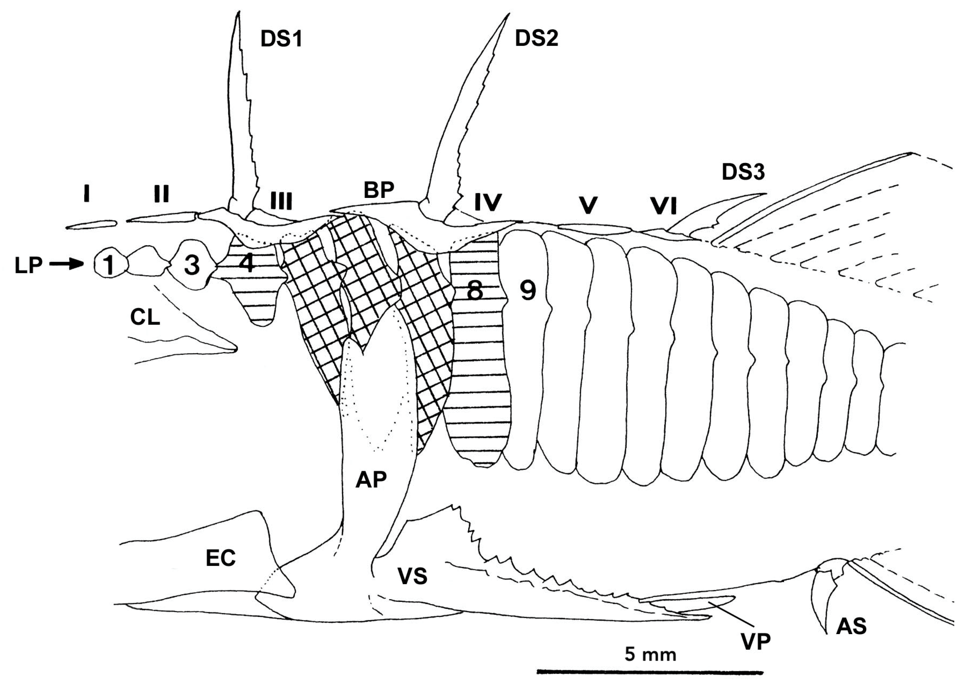
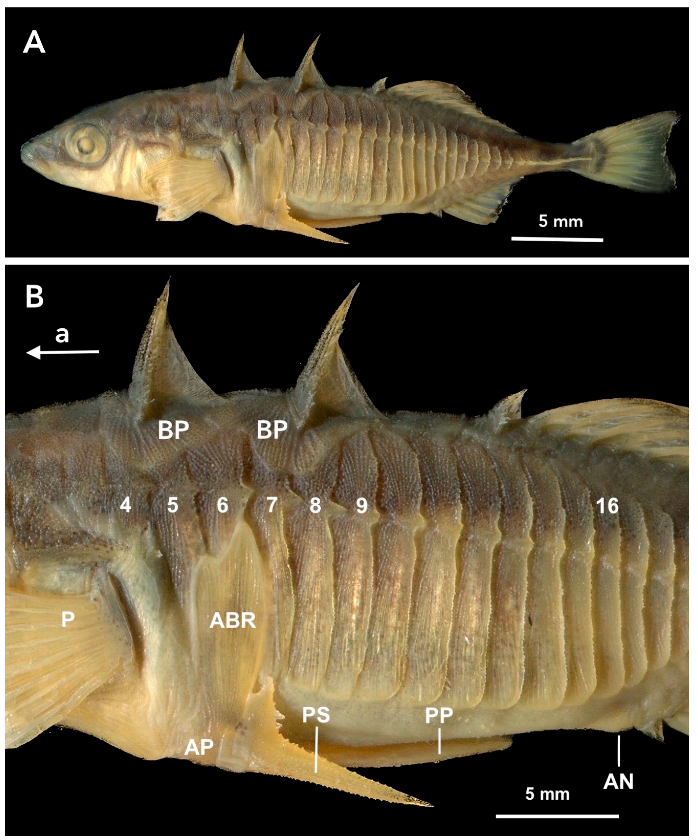
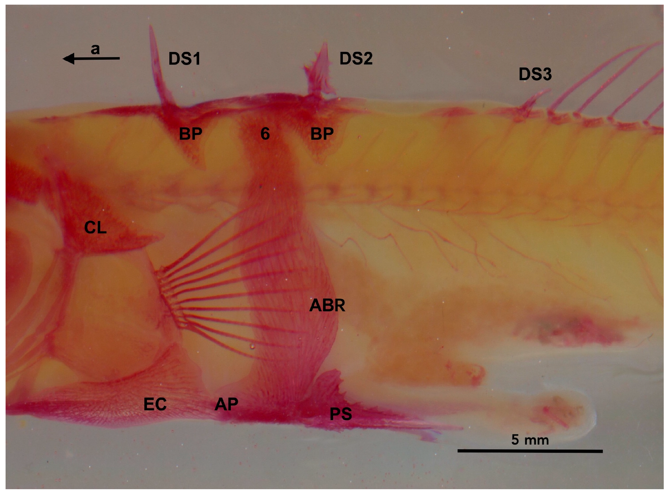
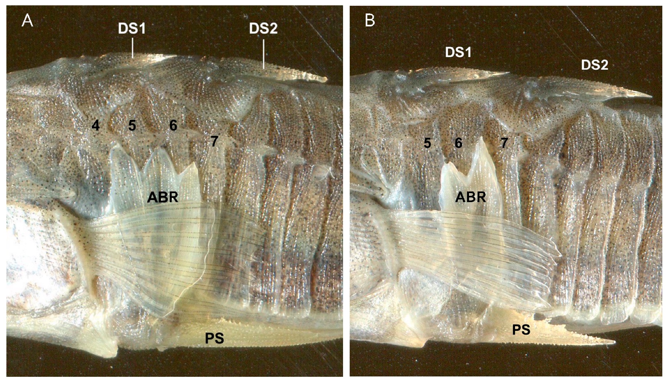
2.4. The Defensive Complex (DC)

The DC is a post-capture defense of bony elements that surrounds the anterior part of the abdomen in a ring-like manner. It consists of the first two dorsal spines, their basal plates, the pelvis with the pelvic spines, and the associated lateral plates (Figure 1; [31,50]). This complex aids against injuries of the skin and underlying muscles during capture and against compression of the internal organs. The completely developed DC typically consists of 20 bony elements combined into three units: (1) the dorsal unit with the first and second dorsal spines along with their basal plates (pterygiophores), (2) the lateral unit with the lateral plates 4–8 and the ascending branch of the pelvis, and (3) the ventral unit with the pelvis (paired) and the two pelvic spines (the pelvic complex). A completely developed DC is separated in two sections, a central and a peripheral one [49]. The structural lateral plates of the central defensive complex (CDC) generally comprise plates 5, 6 and 7. These plates dorsally buttress the first and second dorsal spines and ventrally the ascending branch of the pelvis. The lateral plates anterior and posterior to them, plates 4 and 8, only buttress the first dorsal spine (plate 4) and the second dorsal spine (plate 8), but not the ascending branch of the pelvic complex and are therefore part of the peripheral DC (Figure 1). In our study, we focus solely on the paired elements of the DC, i.e., the structural lateral plates and the pelvic complex.

2.4.1. Structural Lateral Plates

We define those lateral plates as structural plates that connect and support the dorsal and ventral parts of the DC. In a typically completely developed DC, five paired structural lateral plates (typically 4–8) extend on each side in the anterior part of the abdomen (Figure 1). This number can increase if additional plates support the dorsal parts of the DC, e.g., the plates on position 9 (Figure 2). These lateral plates buttress the basal plates that carry the first and second dorsal spines and, in part (plates 5–7), the ascending branch of the pelvis (Figure 1 and Figure 2). In this manner, the forces acting on the fish during an attack of a gape-limited predator on the first and second dorsal and the pelvic spines become distributed over the whole DC [31,32,49]. To avoid ontogenetic bias, we only considered specimens > 34 mm SL (=standard length), at which size lateral plate development is completed [74,75].

Some studies found directional asymmetry in the total plate number [35,36,37]. On a closer look, DA solely resulted from a divergent number of posterior non-structural plates (and not from a divergent number of structural lateral plates). The number of posterior non-structural plates has mainly been linked to swimming behavior [26,53]. Because structural plates are less variable in their positional asymmetry than non-structural plates [7,29,58,59], and to avoid any bias by adaptation to a preferred swimming mode, we focused solely on the structural lateral plates, i.e., the plates included into the DC. These plates face the most physical stress during handling by a predator [31].

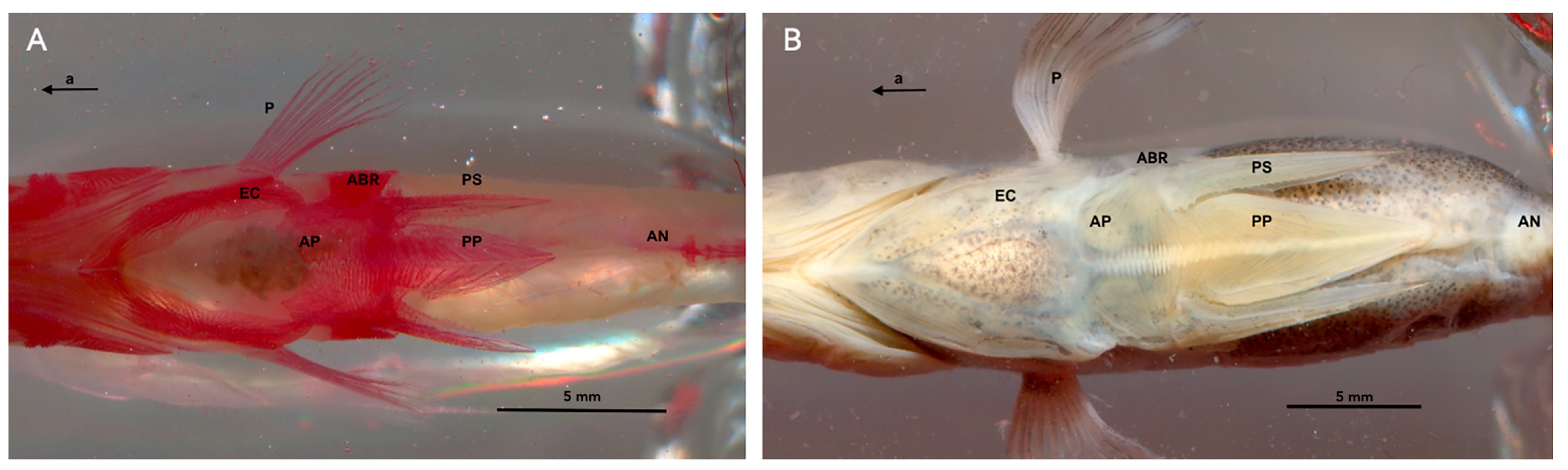
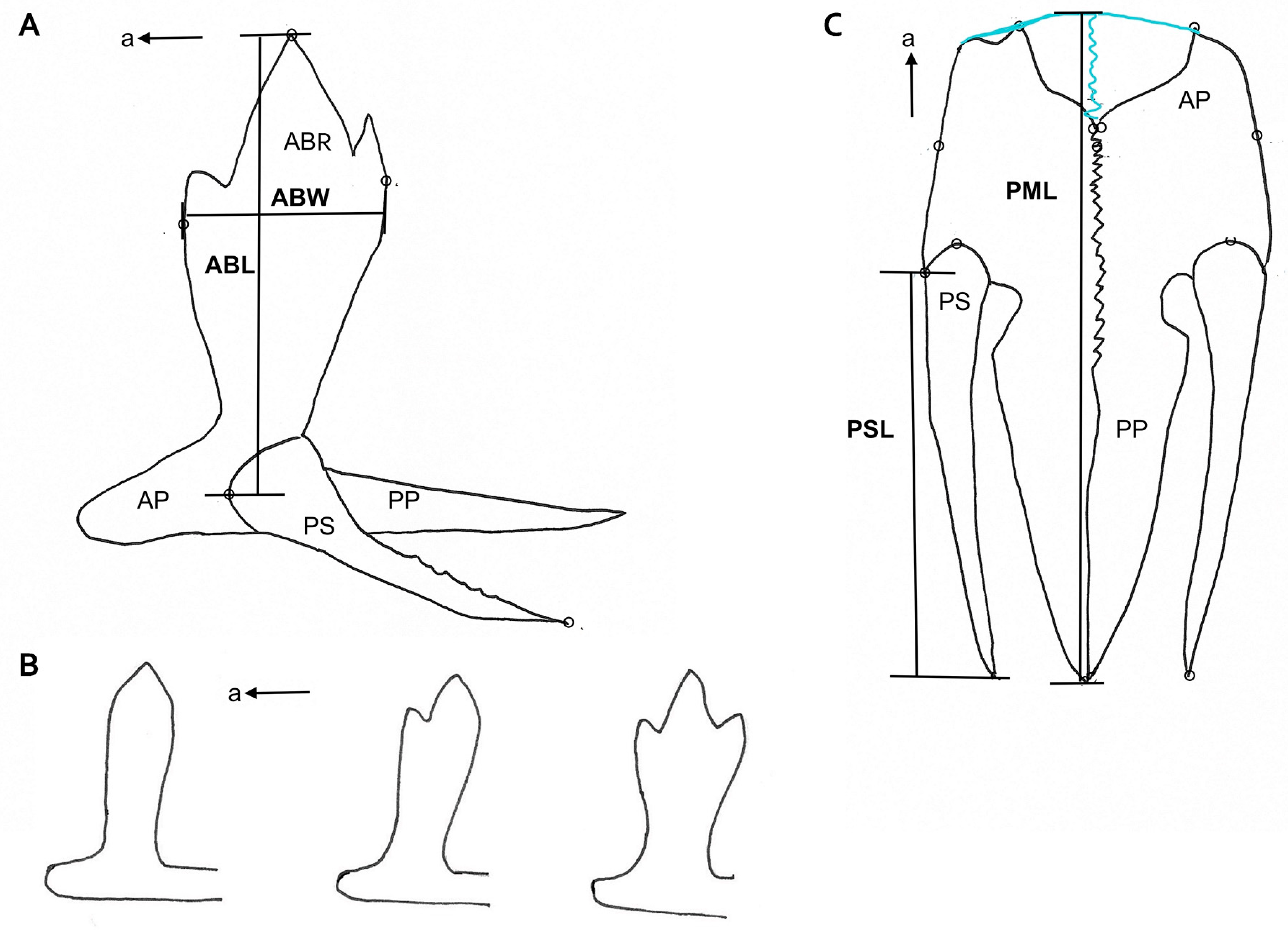
2.4.2. The Pelvic Complex

The pelvic complex consists of the pelvis (a bilateral structure of two medially sutured bony plates) and the two spines of the pelvic fin (pelvic spines) inserted by a joint [21]. Three processes of the pelvis are distinguished: the lateral ascending branch as well as the anterior and the posterior processes of the ventral pelvic plate [31,32,66] (Figure 3). We consider the entire length of the pelvic plate and do not differentiate between the anterior and posterior process. Nevertheless, to avoid confusion with the term “anterior process”, we term the ascending process “ascending branch” [21,61]. Furthermore, we measured along the midline of the pelvis because the anterior edge varied considerably in the four investigated populations—from convex to distinctly concave (Figure 4).

2.5. Data Acquisition

For counting the plates and the forks, fishes were inspected under a binocular microscope (Wild Heerbrugg M5), from the left and right side. To assess the asymmetry of the pelvic complex, the fishes were scanned on a flatbed scanner [76] from both sides and from ventral. Traits were digitally measured on the obtained images using tpsDig2 [77]. Altogether, we took four measurements from four bony structures of the pelvic complex. Two measurements were taken from the lateral side of the pelvis: the length and the width of the ascending branch (ABL and ABW, Figure 4A). Two measurements were taken from the ventral side of the pelvic complex: length of the pelvis in midline (PML) and length of the pectoral spine (PSL, Figure 4A). All measurements are given in mm. Standard length (SL) is defined as the distance from the tip of the snout to the end of the vertebral column. The measurements were taken twice using a digital caliper (±0.01 mm). The mean of the measurements was used. Two addition characters were counted: the number of the structural lateral plates (Figure 2) and the number of forks of the ascending branch of the pelvis (Figure 4B), which are generally associated with the width of the branch.

2.6. Statistical Analyses

Standardized left–right differences were calculated as follows: (L − R)/((L + R)/2). For population comparisons of metric traits, we used a one-way ANOVA or its nonparametric equivalent, the Kruskal-Wallis test. When the number of numerical categories was low, comparisons were realized through Pearson Chi Square tests. Standardized residuals of ±1.96 are to be interpreted as significantly contributing to the overall chi-square statistic [78]. Furthermore, relative variability was calculated by dividing the standard deviation by the mean. This coefficient of variation, also known as relative standard deviation, is reported as a percentage and allows comparing variability between disparate groups and traits. Testing for equality of coefficients of variations from two or more populations was realized following [79], as implemented in the cvequality package in R by [80]. For non-normally distributed data, the Siegel-Turkey test was used instead, with 100,000 permutations. Directional asymmetries were tested with one sample t-tests. p-values are two-tailed, and the overall significance level is 0.05. We used IBM SPSS Statistics (Version 25 and Version 27), PAST (Version 3, [81]), and R (Version 3, [82]) together with the packages cvequality [80], jmuOutlier [83], as well as BoxPlotR (http://shiny.chemgrid.org/boxplotr/, accessed 10 September 2020). Pelvis shape comparisons were performed using the geometric morphometric toolkit with a Procrustes superimposition of the 2D coordinates of the four relevant measurement points [84], followed by a permutational one-way multivariate analysis of variance (MANOVA). Subsequent pairwise tests were reported with Bonferroni corrections. Procrustes superimposition and the graphical realization of individual and group differences were realized in Morpheus et al. [85].

3. Results

Loss of bony elements forming the DC affected only the number of structural lateral plates. All other elements—the first two dorsal spines and their supporting basal plates (pterygiophores) as well as the pelvis with the pelvic spines—were present in all populations. The three processes of the pelvis were developed in all specimens, although to different extents. The reduction of the anterior process in populations under low and moderate predation pressure changed the shape of the anterior part of the pelvis: its margin is normally distinctly concave, but became almost straight in most specimens under high and very high predation pressure. The relevant shape information is depicted in Figure 5. An overall permutational MANOVA showed significant group differences (p = 0.0001, 9999 permutations). Pairwise-tests with Bonferroni adjustments showed that the both the populations under lower predation pressure, AB and HN, as well as the two populations under higher predation pressure, LK and FB, do not differ significantly in shape (p = 0.462 and p = 1.000). All other pairwise comparisons were statistically significant with p = 0.0006.

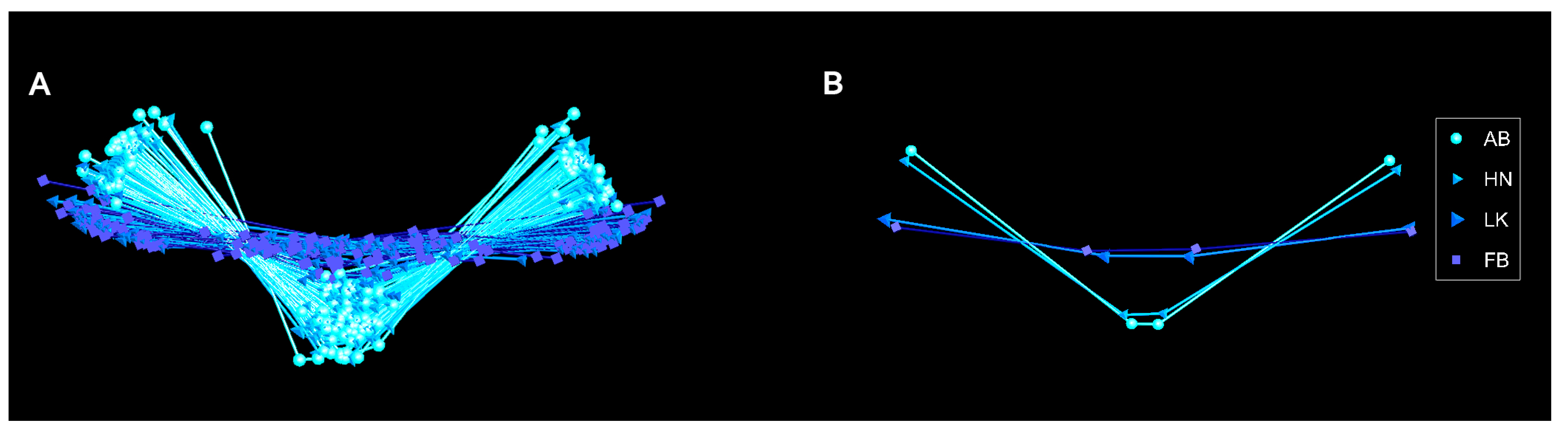
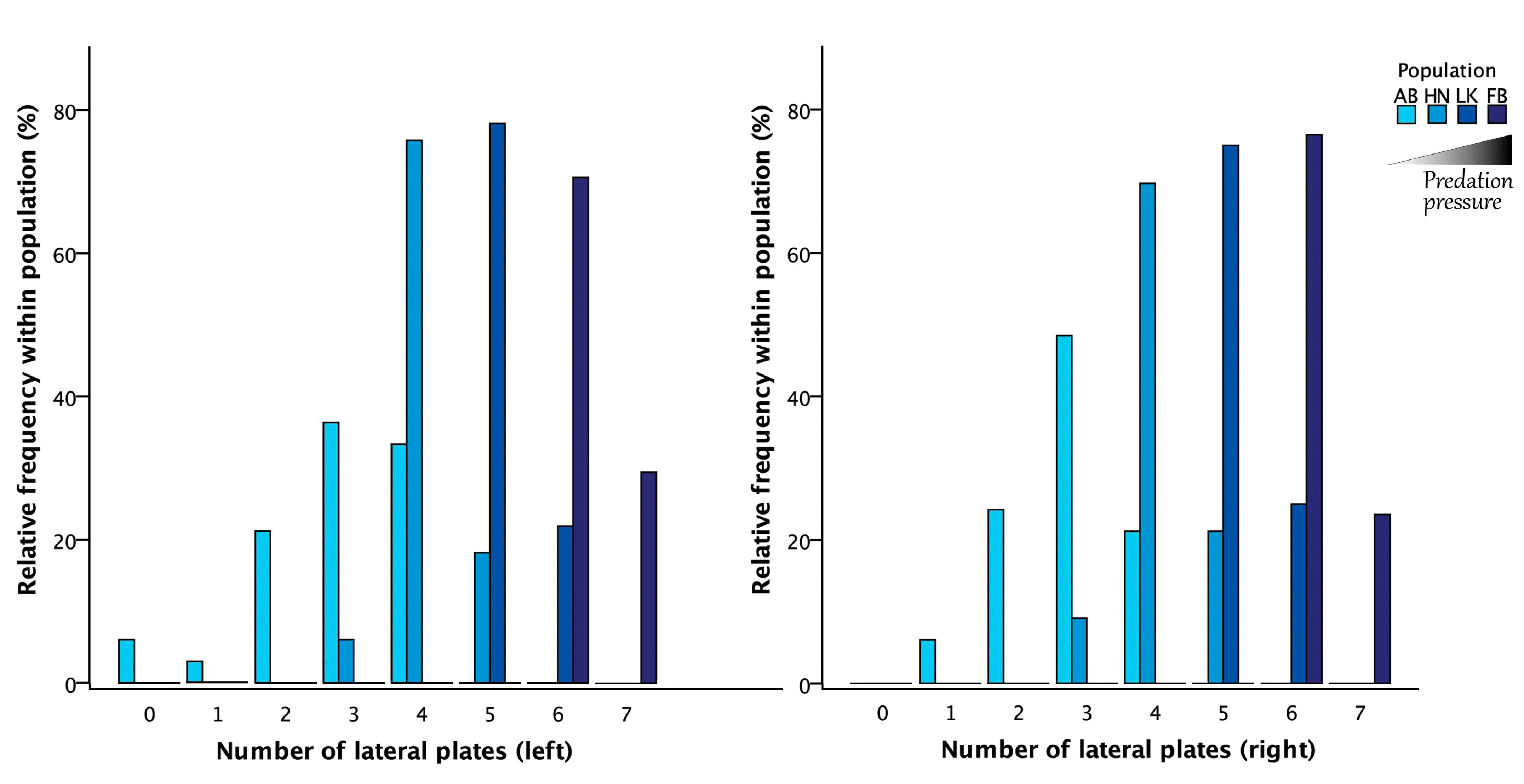
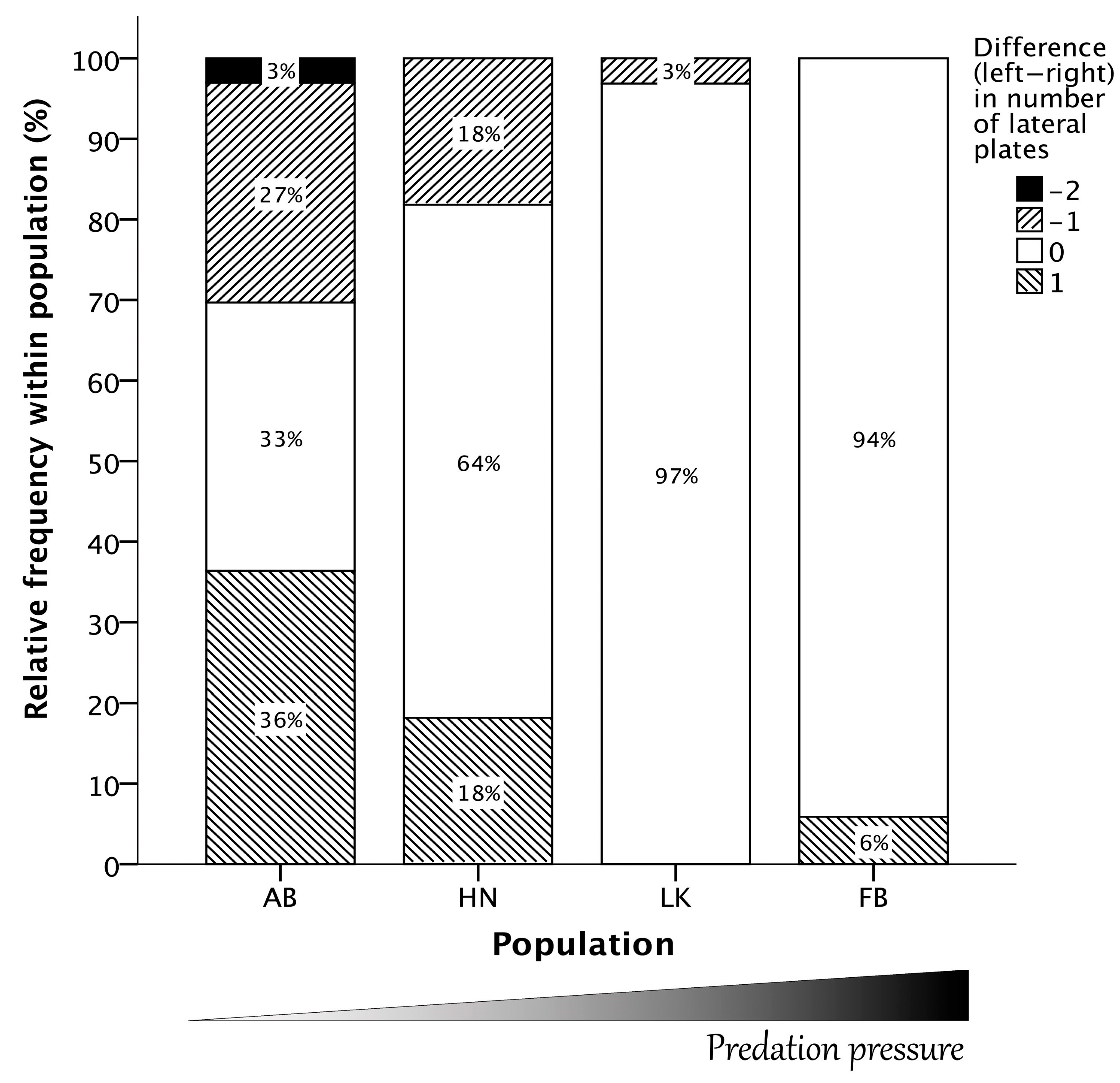
3.1. Symmetry Analyses of the Structural Lateral Plate Numbers

The number of structural lateral plates differed between all four populations, with high numbers of structural plates in the populations from habitats with many predatory fish species (LK, FB) and, in case of the lake population (FB), also predatory birds, and decreasing numbers in the populations with moderate (HN) and low predation pressure (AB). A drastic reduction of structural plates in the AB population led to the nearly complete functional loss of the DC in many specimens. Distributions are given in Figure 6.

The highest number of structural lateral plates was recorded in the lake population FB. The means of the left and right sides averaged 6.3 lateral plates, with an averaged SD of 0.45. The lowest number of functional plates was counted in the stream population AB (M = 2.6, SD = 1.16). Reduced lateral plate numbers (and thus reduced effectiveness of the DC as a unit against gape-limited predators) was evident in the two stream populations with moderate (HN; M = 4.1, SD = 0.51) and low (AB) predation pressure. We also found distinct differences in plate numbers between the populations under high predation pressure, with the sticklebacks from the lake population FB having a more structural lateral plates than those from the stream population LK (M = 5.2, SD = 0.43). A Welch ANOVA (left side: F = 162.0, p < 0.001; right side: F = 191.8, p < 0.001) and pairwise Tamhane’s T2 tests (Appendix A) confirmed that all populations are significantly different. Moreover, intraspecific variation was significantly different between populations (left side: D’AD = 149.85, p < 0.001; right side: D’AD = 93.02, p < 0.001). The lower the predation pressure, the more variable the number of lateral plates: AB showed by far the largest variation, followed by HN, LK, and FB (

Table 1. Descriptive statistics and pairwise population differences in the coefficient of variation.

	Number of Lateral Plates				Pairwise-Tests
Population	Sample Size	Mean	Standard Deviation	Coefficient of Variation (%)	D’AD	p-Value (Uncorrected)
	Left side of the fish
AB	33	2.89	1.11	38.6	AB–HN: 32.27	1.34 × 108
HN	33	4.12	0.48	11.8	HN–LK: 4.31	0.038
LK	32	5.22	0.42	8.0	LK–FB: 0.07	0.012
FB	34	6.29	0.46	7.3
	Right side of the fish
AB	33	2.85	0.83	29.3	AB–HN: 16.72	4.34 × 105
HN	33	4.12	0.55	13.2	HN–LK: 6.16	0.013
LK	32	5.25	0.44	8.4	LK–FB: 1.18	0.277
FB	34	6.24	0.43	6.9

).

There was no directional L–R asymmetry in the structural plates in any of the four populations, and almost perfect symmetry in populations facing high predation pressure (LK, FB; Figure 7). At moderate predation pressure, e.g., in HN, the maximum plate difference was one, with the higher value being equally distributed between both sides. Such asymmetries occurred in one-third of the sampled HN individuals, whereas the other two-thirds were symmetric (Figure 7). Low predation pressure, as in AB, was associated with two-thirds of the population showing an asymmetric count and only one-third the symmetric count (Figure 7). One individual even displayed a difference in the two plates between its left and right sides. Combined, the higher the predation pressure, the less L–R asymmetry was observed in the lateral plate number in the defensive complex.

3.2. Symmetry Analyses of the Pelvic Complex

In terms of L–R asymmetries within the pelvic complex, we found no convincing evidence for directional asymmetries in the four populations (Figure 8,

Table 2. One-sample t-tests per trait in the pelvic complex and population. The standardized left–right differences are compared against a mean value of 0. All p-values are uncorrected and two-sided. After Bonferroni correction, no relevant directional asymmetries remain.

Population	Trait	t	df	p
AB (n = 32)	Pelvic spine length (PSL)	−2.4	31	0.021
	Pelvic length (PML)	0.8	31	0.459
	Ascending branch width (ABW)	−0.9	31	0.390
	Ascending branch length (ABL)	0.9	31	0.350
HN (n = 34)	Pelvic spine length (PSL)	−0.8	33	0.435
	Pelvic length (PML)	0.1	33	0.889
	Ascending branch width (ABW)	0.3	33	0.778
	Ascending branch length (ABL)	−1.8	33	0.088
LK (n = 31)	Pelvic spine length (PSL)	−2.2	30	0.038
	Pelvic length (PML)	0.8	30	0.428
	Ascending branch width (ABW)	2.1	30	0.040
	Ascending branch length (ABL)	0.3	30	0.794
FB (n = 33)	Pelvic spine length (PSL)	−0.9	32	0.359
	Pelvic length (PML)	0.6	32	0.576
	Ascending branch width (ABW)	−1.3	32	0.205
	Ascending branch length (ABL)	−1.2	32	0.255

).

There were, however, significant differences in the magnitude of L–R asymmetries in the pelvic complex between the four populations (Figure 9). The populations differed significantly with regard to the left–right difference in the length of the pelvis in midline (PML, Kruskal-Wallis H = 34.26, p < 1.75 × 10⁷) and the width of the ascending process (ABW, Kruskal-Wallis H = 10.17, p = 0.017). This was not the case for pelvic spine length (PSL, Kruskal-Wallis H = 5.33, p = 0.149) or ascending process length (ABL, Kruskal-Wallis H = 0.70, p = 0.874). If one considers the result for PSL a trend, then this trend is rooted in the difference between AB and FB—the two extremes in terms of predation pressure.

For PML, pairwise comparisons with Bonferroni correction showed that the two populations of low predation pressure, AB and HN, were not significantly different from each other. Moreover, the two populations with high predation pressure, LK and FB, did not differ significantly from each other. All other pairwise comparisons were significant with p-values less than 0.001 after Bonferroni correction, indicating that high predation pressure is related to less asymmetry.

For ABW, pairwise tests remained significant after Bonferroni correction between HN and FB only (p = 0.045), with higher values for FB; there might be a trend for a difference between AB and FB (p = 0.149 after Bonferroni correction, uncorrected p = 0.025), again higher values for FB. Thus, ascending process width becomes increasingly asymmetric with very low as well as with very high predation pressure. This called for further investigations of the defensive complex: we therefore counted the number of overlapped lateral plates as well as the number of forks as additional defensive measures and compared them between populations (Section 3.3). In terms of intraspecific variation of the left–right differences, only PML showed significant population differences (

Table 3. Results of the Siegel–Tukey tests to see if one population has more widely dispersed standardized-left–right differences in the length measures of the pelvic complex than the other. All p-values are uncorrected and two-sided. Applying Bonferroni correction per trait, the new significance level is p ≤ 0.008. Rank sums are included for significant differences only.

	PML				ABW
Population	AB	HN	LK	FB	AB	HN	LK	FB
AB	-----	0.855	1 × 10−5 a	2 × 10−5 b	-----	0.955	0.133	0.030
HN	0.321	-----	4 × 10−5 c	3 × 10−5 d	0.690	-----	0.176	0.010
LK	0.695	0.912	-----	0.964	0.729	0.139	-----	0.270
FB	0.130	0.488	0.469	-----	0.639	0.724	0.248	-----
	PSL				ABL

Rank sums (lower rank => more dispersed): ^a AB 703.6, LK 1312.4; ^b AB 730.625, FB 1414.375; ^c HN 811.5, LK 1333.5; ^d HN 822.5, FB 1455.5.

). Here, the populations under lower predation pressure (AB, HN) were significantly more variable than the two populations under higher predation pressure (LK, FB).

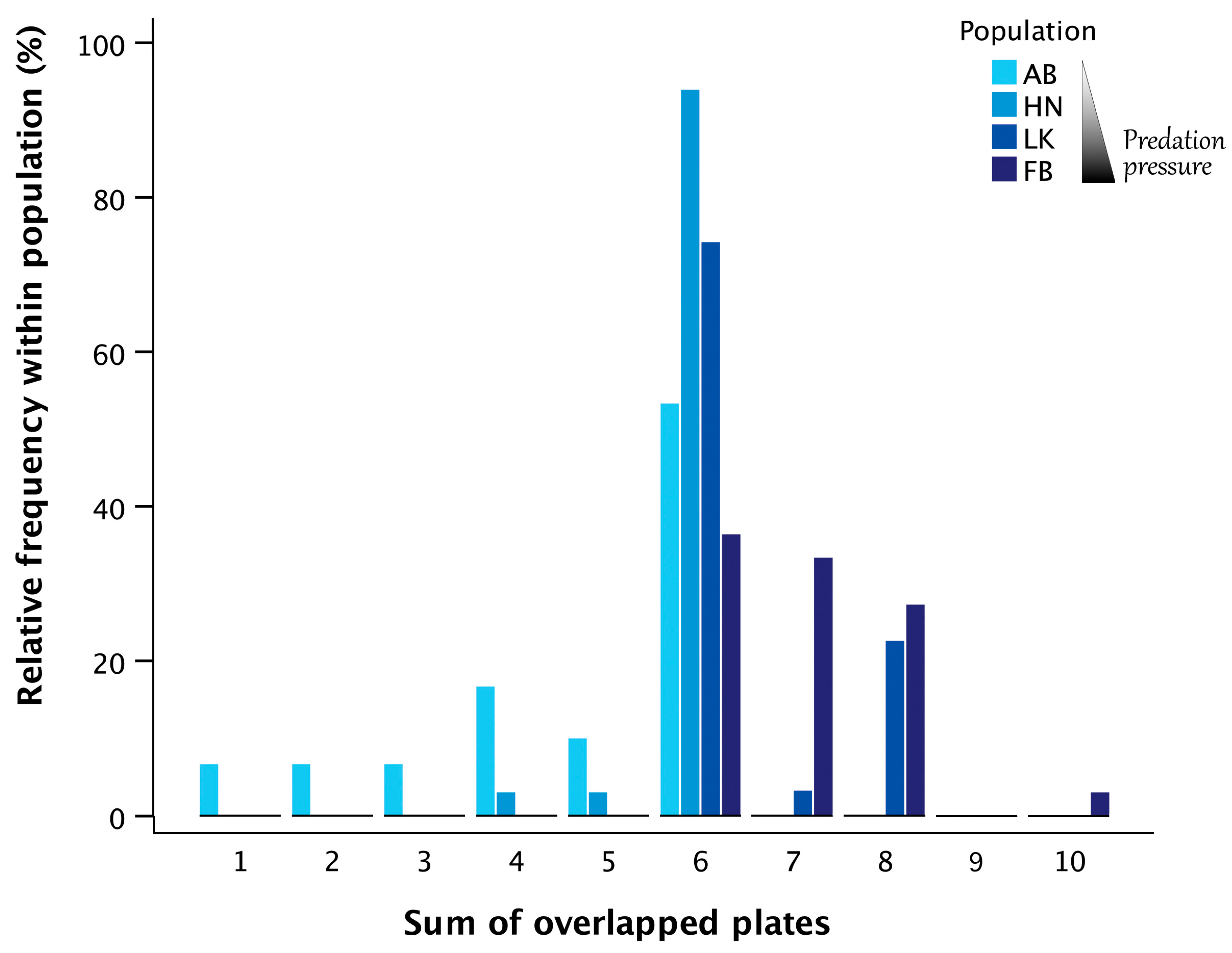
3.3. Symmetry Analyses of the Structural Plates of the Central Defensive Complex (CDC)

The numbers of structural plates of the CDC simultaneously overlapped dorsally and ventrally by the ascending branch of the pelvic complex differed significantly between populations (Kruskal-Wallis H = 50.48, p < 0.001, n = 127). Pairwise posthoc tests showed that HN, and especially AB individuals, had significantly fewer plates overlapped than LK or FB specimens (Figure 10 and Figure 11,

Table 4. Pairwise population comparisons in the total number of overlapped plates by the pelvic complex. The populations exposed to lower predation pressure have significantly fewer plates overlapped than fishes of populations under higher predation pressure. The two populations with the lowest predation pressure did not significantly differ from each other in this trait.

Population Difference	Test Statistic	Std. Error	Std. Test Statistic	Sig.	Adj. Sig. a
AB–HN	−20.342	7.921	−2.568	0.010	0.061
AB–LK	−38.390	8.042	−4.774	<0.001	<0.001
AB–FB	−57.509	7.921	−7.260	<0.001	<0.001
HN–LK	−18.048	7.854	−2.298	0.022	0.129
HN–FB	−37.167	7.730	−4.808	<0.001	<0.001
LK–FB	−19.119	7.854	−2.434	0.015	0.090

^a Significance values adjusted by Bonferroni correction for multiple tests.

).

FB individuals tended to have more overlapped plates than LK individuals. The total number of such plates by population is given in Figure 11. Both reduction and increase were achieved basically in a symmetric manner. In HN and LK, 97% of the individuals were symmetric with regard to the number of overlapped plates. In AB, the value was 83%, and in FB, 67%. Left and right sides differed by a maximum of one plate only in all populations (Appendix B). If there was one overlapped plate, it was plate number 6. In the case of two, either the fifth or the seventh plates were added. In the case of three overlapped plates, numbers 5, 6 and 7 were covered. In the case of four plates, plate number 8 was added, and the individual that had five plates covered at each side had plates 4 to 8 overlapped by the pelvic complex.

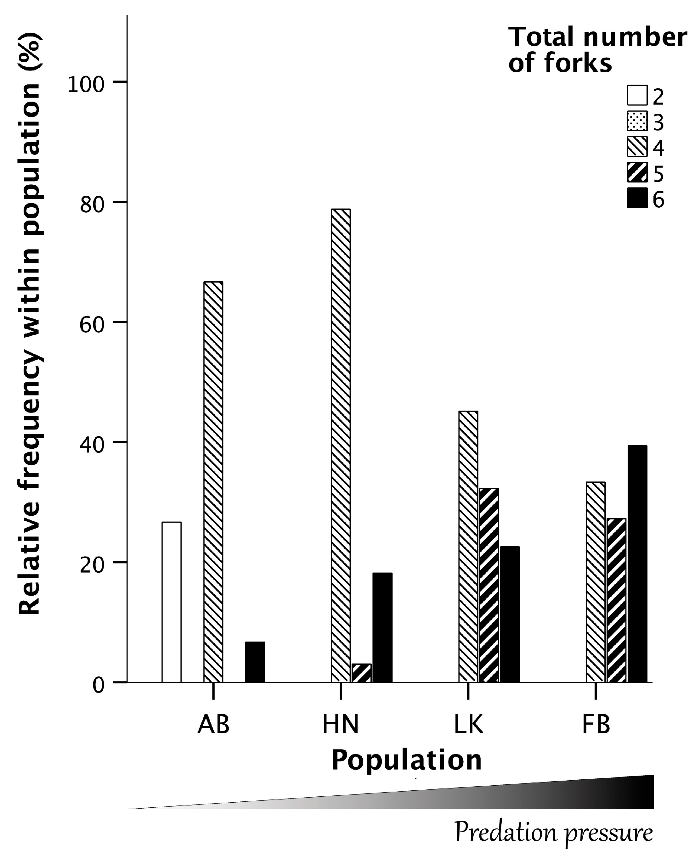
3.4. Symmetry Analyses of the Forks of the Ascending Branch of the Pelvis

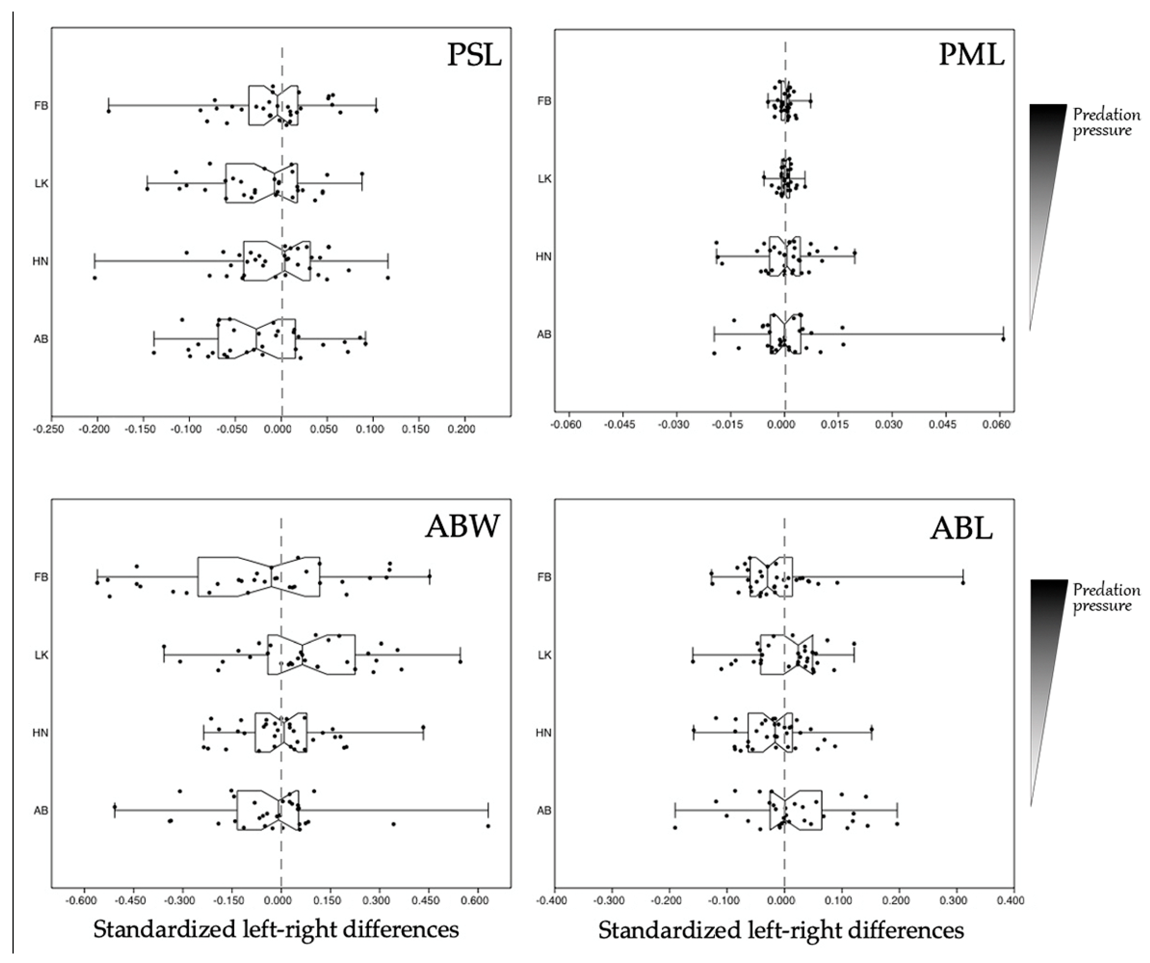
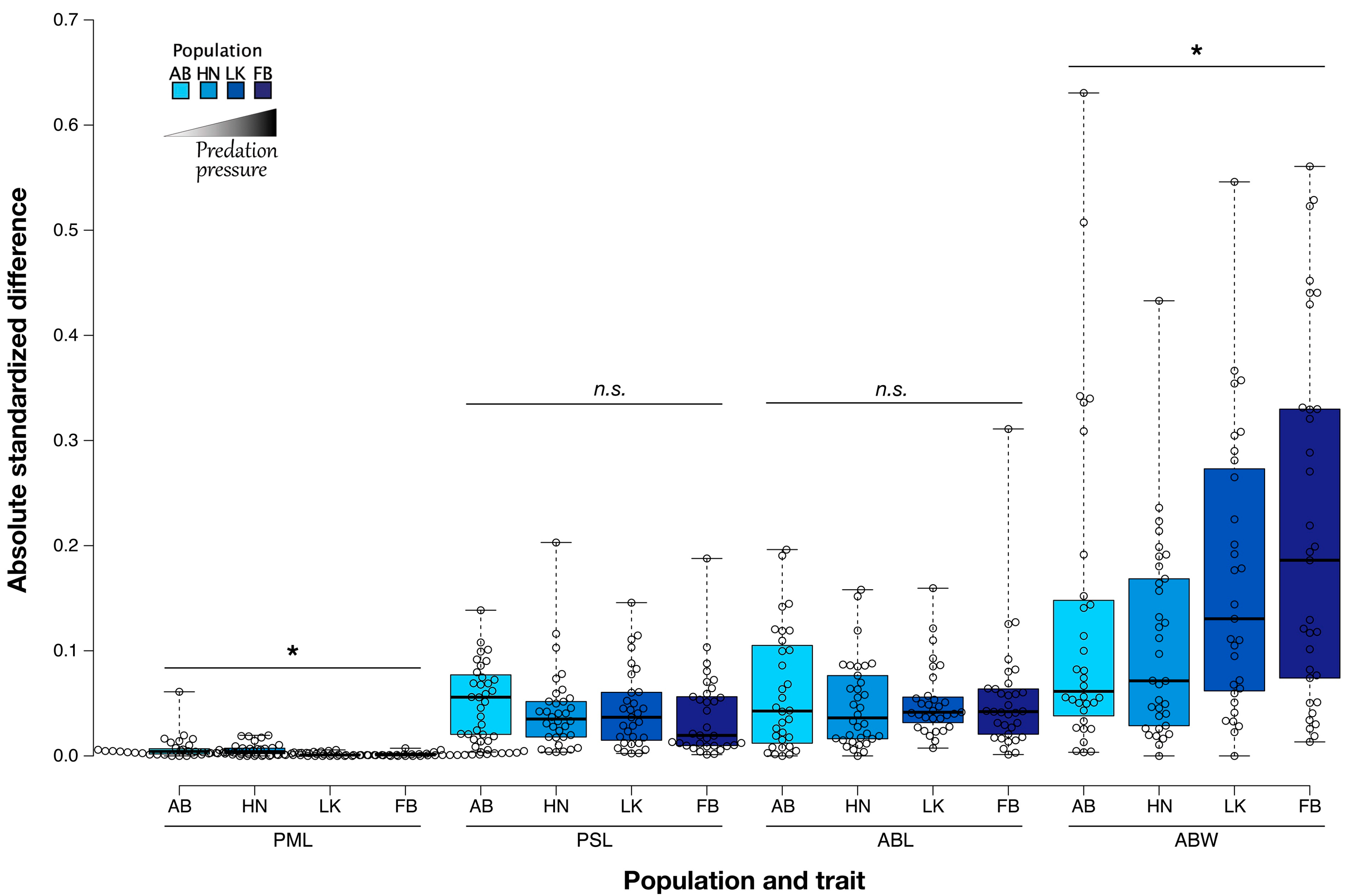
In AB, 8 individuals (27%) had a total number of two forks. All other individuals had at least four forks (Figure 12). In order to meet the requirements for a Pearson Chi-Square test, only the latter were included in the statistical analyses. The test confirms that the four populations differ significantly in the total number of forks in the ascending branches (Χ² = 30.42, p < 0.001, n = 119).

Standardized residuals showed that low and moderate predation pressure was associated with a predominance of four forks, whereas higher predation pressure was associated with a higher total number of forks and fewer individuals with four forks only (Figure 13,

Table 5. Cross-tabulation of population versus the total number of forks in the ascending branch. Fewer forks were significantly associated with low predation pressure and vice versa. Significance within cells is indicated by a standardized residual larger than 2 (in absolute value, bold-face).

			Total Number of Forks			Total
			4	5	6
Population	AB	Count	20	0	2	22
		Expected count	13.1	3.7	5.2
		% within population	90.9	0.0	9.1
		Std. residual	1.9	−1.9	−1.4
	HN	Count	26	1	6	33
		Expected count	19.7	5.5	7.8
		% within population	78.8	3.0	18.2
		Std. residual	1.4	−1.9	−0.6
	LK	Count	14	10	7	31
		Expected count	18.5	5.2	7.3
		% within population	45.2	32.3	22.6
		Std. residual	−1.0	2.1	−0.1
	FB	Count	11	9	13	33
		Expected count	19.7	5.5	7.8
		% within population	33.3	27.3	39.4
		Std. residual	−2.0	1.5	1.9
Total		Count	71	20	28	119

). The decrease and increase in forks were realized primarily in a symmetric manner. No fish had more than one fork difference between its left and right sides (Appendix C).

3.5. Pelvis Length

The populations differed significantly in the length of the pelvis (PML) relative to SL (F = 103.28, p < 0.001). All pairwise comparisons between populations were statistically significant after Bonferroni correction (all p < 0.001) with the exception of LK versus FB (here p = 1.000). Thus, LK and FB had the longest PMLs relative to SL, followed by HN and AB. Accordingly, the relative length of PML decreases in populations with lower predation pressure. Intrapopulation variation was higher in populations with lower predation pressure (D’AD = 16.70, p = 8.14 × 10⁻⁴). HN was the most variable (SD was 11.8% of the mean), followed by AB with 10.9%. LK varied significantly less (7.6%) than HN, but somewhat more than FB (7.5%). Detailed test statistics are given in

Table 6. Descriptive statistics and population comparisons for intrapopulation variation for ventral length measures of the pelvic complex relative to SL. For this, pelvic length and pelvic spine length were divided by SL.

	Descriptive Statistics (%)				Pairwise-Tests
Population	Sample Size	Mean	Standard Deviation	Coefficient of Variation	D’AD	p-Value (Uncorrected)
	Pelvic length/standard length
AB	32	18.22	1.99	10.9	AB–HN: 4.05	0.044
HN	34	20.42	1.56	11.8	HN–LK: 4.58	0.032
LK	31	24.18	1.25	7.6	LK–FB: 4.30	0.038
FB	33	24.48	1.84	7.5
	Pelvic spine length/standard length
AB	32	11.63	1.37	11.8	Overall test n.s.
HN	34	13.80	1.40	10.2
LK	31	15.42	1.29	8.4
FB	33	14.85	1.57	10.6

.

3.6. Pelvic Spine Length

A similar pattern was evident for relative pelvic spine length (F = 44.20, p < 0.001). All pairwise comparisons between populations were statistically significant after Bonferroni correction (all ps ≤ 0.018) with the exception of LK versus FB (here p = 0.679). In LK and FB, the pelvic spines were relatively larger than that in HN. HN, in turn, showed relatively larger pelvic spines than AB (Table 6). The coefficient of variation was not significantly different between populations (D’AD = 3.40, p = 0.333). The standard deviations range between 8.4% and 11.8% of the respective means (Table 6).

3.7. Fish Size

The four populations differed significantly in standard length (Kruskal-Wallis H = 89.47, p < 0.001). All pairwise comparisons were significant with an adjusted p-value of 0.033 or less. HN was the smallest population, followed by AB, LK and FB (

Table 7. Descriptive statistics of fish length (standard length, SL) per population.

Population	Percentiles SL (in mm)			n	Predation
	25	50	75		Pressure
AB	43.2	45.1	48.4	32	low
HN	36.7	37.4	38.3	34	moderate
LK	47.9	49.8	51.8	31	high
FB	51.4	57.2	60.8	33	very high

). Comparing the three stream populations, size was apparently correlated with the size of the habitat. The Lustenauer Kanal (LK) is the widest and deepest stream, the Neubach (NB) the narrowest and shallowest. These differences suggest that size was correlated to the habitat and not to predation.

4. Discussion

Our results showed that increasing size, number and symmetry of the paired elements of the defensive complex (DC), a post-capture defense, of the threespine stickleback, occur in populations under divergent amounts of potential predators, from very low (AB) to many (FB). It appears that the number of potential predators is a more important driver of population differences in the development of the DC than the intensity of predation [32].

In general, high predation pressure from gape-limited fishes tends to result in a reinforced DC [31,32], while a reduction in predatory pressure leads to a reduction in this defense structure. Although water birds (beaked predators) are likely predators in the lake (FB) and the canal (LK) habitats, avian predation, which is often associated with a reduction in the number of lateral plates (non-structural and structural) [7,32], is possibly less distinct compared to predation by numerous piscivorous fish species (toothed predators). However, threespine sticklebacks from LK and FB habitats show no reductions in the number of structural plates. On the contrary, the number of these plates increased beyond the typical five in the lake population. Moreover, birds are highly mobile and have easy access to water bodies, if they are located nearby like the two small brooks that have threespine sticklebacks with a reduced DC. It is expected that avian predation would have led to a similar morphology of the DC in both populations; however, the specimens from these two habitats do differ distinctly in the number of structural plates. Moreover, we found no individuals with predator-induced injuries caused by bills of birds such as lacerations or spine fractures [32].

When high predation selects for a reinforced DC [31,32], relaxed predation should allow for a less costly, reduced DC. This is what we found: a reinforced DC in habitats with many potential predators (FB, LK), and a reduced DC, which was even further reduced, respectively, in the populations with a low (HN) or very low (AB) amounts of potential predators. Nevertheless, not all elements of the DC were affected evenly. Considerable asymmetry was found in three of five investigated traits: the number of structural lateral plates, the width of the ascending branch of the pelvis and the length of the pelvis. Nearly perfect symmetry occurred in the length of the ascending branch and in the length of the pelvic spines. Although DA in the lateral plate number [36,86] and in the pelvic complex [15,87,88] has been reported for some North American populations, we found no trait that expressed directional asymmetry (DA) in these Austrian populations. Future studies of comparable populations are needed to help deciding if our findings result from low statistical power or the lack of directional asymmetries. Unfortunately, increasing sample sizes for the original populations is not possible, because one population got extinct due to polluted water (AB, the only known one with such reduced armor in Austria) and others were diminished through habitat restructuring.

Studies have shown a stabilizing effect of predation on DC [7,29,31,54,89]. Such predation pressure seems to select for symmetry and canalization (reduced phenotypic variation) in the paired traits that are crucial for the effectiveness of the DC post-capture [7]. Along these lines, we found asymmetries in lateral plate number to decrease along a predatory gradient: two-thirds of the individuals were asymmetric in the population barely exposed to predatory fish (AB) to almost purely symmetric individuals in the two populations with the highest predatory pressure (LK, FB). The population under moderate predatory pressure (HN) was intermediate, with one-third of the sampled fish being asymmetric. This fits with the stabilizing selection of predation on defense structures [36,89], which is clearly also repressing intrapopulation variation. The highest variation was observed in the population with low predation risk and with an ineffective DC. This suggests that the rapid increase in variation and asymmetry was linked to a major reduction of the function of the DC. Despite this, all but one of the examined asymmetric specimens had a single plate difference between the left and right sides only, which is also seen in a North American lake population [15].

Relative length measures showed that standardized left–right differences were more dispersed in populations with lower predatory pressure when it came to the length of the pelvis in the midline. No such differences were observed for pelvic spine length and the two linear measures of the ascending branch. Furthermore, the length of the pelvic spines and the length of the ascending branch in the pelvic complex showed no population differences in asymmetry. In contrast, asymmetry in the length of the pelvis at the midline increased when predatory pressure is low. Against expectations, the opposite pattern appeared for the asymmetry of the width of the ascending branch, which increased with increasing predatory pressure. Thus, the investigated morphological traits of the pelvic complex responded differently along a predatory gradient. It remains unclear why the width of the ascending branch showed population differences in asymmetry but the length did not. For example, in Canadian populations (Haida Gwaii Island), the length of the ascending branch had the highest level of asymmetry (FA) [38]. Generally, the width of the ascending branch was associated with the number of forks. A narrow ascending branch ends in a single fork, while a wide branch ends in up to three forks [38,88]. The increase of predation pressure clearly favored an increase in fork width and number. In populations with a high total number of forks per individual (LK, FB), significantly more individuals were asymmetric when comparing the number of forks between the left and right sides. Thus, high predatory pressures might have led to a strengthening of the DC by increasing ascending branch width and fork number in these populations, at the cost of bilateral symmetry in these traits. Lacking longitudinal samples across many generations, it remains unclear whether the observed condition represents a transitory stage ultimately ending in symmetric individuals with a more potent DC, or whether concurring costs favor a certain number of asymmetric individuals in the population over the long run. In the lake population (FB, highest predation pressure), not only did the number of structural plates and therefore the area of the abdomen covered by the DC increase, but the number of these plates that were overlapped by a wider ascending branch also increased. Again, this was associated with a higher percentage of individuals, i.e., one-third, having an asymmetric count of overlapped plates. In contrast, the other two stream populations under high (LK) and moderate (HN) predation pressure were almost entirely symmetric. The stream population with low predatory pressure (AB) was intermediate (one-fifth asymmetric). The increase in width and fork number is in accordance with an increased resistance against compression of the abdomen post-capture and generally correlates to predation pressure [38,89].

Asymmetry in pelvis length, however, could result from its decrease in length. Piscine predation is known to affect pelvis length, which is longer under high predation pressure [89,90,91]. A short pelvis, leaving large areas of the abdomen uncovered, is generally found in populations with low predation pressure. This pattern was confirmed in our findings on relative pelvic length. In populations with a shorter pelvis, we also identified concave—as opposed to straight—anterior pelvic outlines. Straight anterior outlines afford more bony investment, but increase stability and protection, which seemed, together with an overall longer pelvis, worthwhile in the two populations in habitats with many predatory species. Apparently, relaxation of this pressure resulted not only in a relative shortening of the pelvis, but also in L–R asymmetries. Similarly, for the overall number of structural lateral plates, variability was the highest in the populations with relaxed predation pressure.

Such variations along a predatory gradient in traits that are important for the effectiveness of the DC post-capture suggest an ongoing ecological process, reflecting adaptation to different predatory pressure. Reduced predation resulted, as expected [31,52,54,60,89,90], in gradually fewer structural plates, shorter pelvises with a concave anterior outline, narrower ascending branches, and shorter pelvic spines (see below) in the two populations under low and moderate predation pressure. What was unexpected, however, was that the number of structural lateral plates and the width and number of forks of the ascending process showed significant variation and asymmetry in the lake population, which faced the highest predation pressure. This was surprising because functional structures are under stabilizing selection and are expected to be symmetric if predation is strong [4,15,36,89]. Therefore, clearly, not only a decrease but also an increase of predation pressure may favor L–R asymmetries in the DC of the threespine stickleback.

It also remains unclear why reduced pelvis length was correlated to asymmetry and variability, yet the reduction in pelvic spine length was not significantly so. As expected, pelvic spine length decreased along the predatory gradient because predation favors long spines [89], but there were no significant population differences in asymmetry. This could either reflect the small sample sizes or be the result of assortative mating. Females select male sticklebacks for pelvic spine symmetry [92,93], but not for their lengths [94]. Pelvic spines are important for males not only for defense [31,50], but also for display in agonistic behavior [94,95,96]. Similar considerations might hold true for the ascending branch of the pelvis.

Asymmetries and reductions in the DC have been documented for various populations of the threespine stickleback (e.g., [30,58,64,97]). Such reductions were also found in the ninespine stickleback (Pungitius pungitius (Linnaeus 1758)) and in the brook stickleback (Culaea inconstans (Kirtland 1840)) [12,58,98] and were also attributed to low or absent predation pressure. This parallelism is a strong indication that predation pressure, or the lack thereof, acts selectively on the bony armor of threespine sticklebacks and that it is the main driver of variation, an effect already observed at negligible predation [12].

A reduction in bilateral developed armor traits is apparently often correlated with asymmetries, and some studies found a positive association between asymmetries and fitness [89,99]. Accordingly, reduced bony armor in response to relaxed predation pressure reduces fitness costs and may enable faster growth and earlier maturity [100]. This may also hold true in reverse, i.e., the assemblage of armor traits increases in response to increasing predation pressure by gape-limited predators. Possibly there is a “normative” DC in the number as well as in the size and the shape of paired elements, whereby predation pressure selects for symmetry in these traits within this “optimum” [7,12,26,37]. These traits would then respond with deviations to environmental changes such as predation [3] Nevertheless, some traits seem to be more canalized (e.g., pelvic spines) than others (e.g., structural lateral plates). Moreover, in most studies, “armor” was investigated in a general sense, and if specific elements of the DC were mentioned, non-structural plates were also included in the analysis [88]. These non-structural plates may serve additional purposes such as improving hydrodynamic performance.

We assume that threespine sticklebacks that experienced extremely divergent environmental conditions, i.e., low predation pressure vs. very high predation pressure, were involved in an ongoing ecological process as a result of adaptation to relaxed vs. increased predation. Both reduction and strengthening of the DC in these populations suggest adaptability and increasing fitness. Importantly, our results showed that traits of the DC respond differently to predation pressure and that the asymmetry of traits may not correlate with the asymmetry of other traits. Environmental stress has the potential to increase phenotypic variation and to destabilize development in the threespine stickleback. The shift of this stress may alter complex traits [101], thus influencing the response to selection. Our results show that relaxation of environmental stress, i.e., relaxation of predatory pressure, may have a similar effect. Further investigation is needed to fully understand the impact of the inherent bias in meristic traits on the interpretation of the results [102,103]. Another area for future research is the development of innovative methods to sample for quantifying predators, including the use of remote sensing (e.g., [104,105]) and sonar technologies (e.g., [106,107]). Together with a wider range of populations and an increase in sample sizes, it will then be possible to detect finer details in the patterns of predator–prey interactions and to better understand the mechanisms driving these interactions.

References

1. Palmer, A.R.; Strobeck, C. Fluctuating asymmetry as a measure of developmental stability: Implications of non-normal distributions and power of statistical tests. Acta Zool. Fennica 1992, 191, 57–72. [Google Scholar]
2. Van Dongen, S. Fluctuating asymmetry and developmental instability in evolutionary biology: Past, present and future. European Soc. Evol. Biol. 2006, 19, 1727–1743. [Google Scholar] [CrossRef] [PubMed]
3. Kenney, L.A.; von Hippel, F.A. Morphological asymmetry of insular freshwater populations of threespine stickleback. Environ. Biol. Fish. 2014, 97, 225–232. [Google Scholar] [CrossRef]
4. Van Valen, L. A study of fluctuating asymmetry. Evolution 1962, 16, 125–142. [Google Scholar] [CrossRef]
5. Palmer, A.R. Symmetry breaking and the evolution of development. Science 2004, 306, 828–833. [Google Scholar] [CrossRef] [Green Version]
6. Martin, J.; López, P. Hindlimb asymmetry reduces escape performance in the lizard Psammodromus algirus. Physiol. Biochem. Zool. 2001, 74, 619–624. [Google Scholar] [CrossRef]
7. Bergstrom, C.A.; Reimchen, T.E. Asymmetry in structural defenses: Insights into selective predation in the wild. Evolution 2003, 57, 2128–2138. [Google Scholar]
8. Galeotti, P.; Sacchi, R.; Vicario, V. Fluctuating asymmetry in body traits increases predation risks: Tawny owl selection against asymmetric woodmice. Evol. Ecol. 2005, 19, 405–418. [Google Scholar] [CrossRef]
9. Møller, A.P. Developmental stability and fitness: A review. Am. Nat. 1997, 149, 916–932. [Google Scholar] [CrossRef]
10. Møller, A.P. Asymmetry as a predictor of growth, fecundity and survival. Ecol. Lett. 1999, 2, 149–156. [Google Scholar] [CrossRef]
11. Lens, L.; van Dongen, S.; Kark, S.; Matthysen, E. Fluctuating asymmetry as an indicator of fitness: Can we bridge the gap between studies? Biol. Rev. 2002, 77, 27–38. [Google Scholar] [CrossRef] [Green Version]
12. Trokovic, N.; Herczeg, G.; Ab Ghani, N.I.; Shikano, T.; Merilä, J. High levels of fluctuating asymmetry in isolated stickleback populations. BMC Evol. Biol. 2012, 12, 115. [Google Scholar] [CrossRef] [Green Version]
13. Gummer, D.L.; Brigham, R.M. Does fluctuating asymmetry reflect the importance of traits in little brown bats (Myotis lucifugus)? Can. Zool. 1995, 73, 990–992. [Google Scholar] [CrossRef]
14. Karvonen, E.; Merilä, J.; Rintamäki, P.T.; van Dongen, S. Geography of fluctuating asymmetry in the greenfinch, Carduelis chloris. Oikos 2003, 100, 507–516. [Google Scholar] [CrossRef]
15. Reimchen, T.E.; Bergstrom, C.A. The ecology of asymmetry in stickleback defense structures. Evolution 2009, 63, 115–126. [Google Scholar] [CrossRef]
16. Wootton, R.J. The Darwinian stickleback Gasterosteus aculeatus: A history of evolutionary studies. J. Fish. Biol. 2009, 75, 1919–1942. [Google Scholar] [CrossRef]
17. Campbell, R.N. Morphological variation in the three-spined stickleback (Gasterosteus aculeatus) in Scotland. Behaviour 1985, 93, 161–168. [Google Scholar] [CrossRef] [Green Version]
18. Bell, M.A.; Foster, S.A. The Evolutionary Biology of the Threespine Stickleback; Oxford University Press: Oxford, UK, 1994. [Google Scholar]
19. Kingsley, D.M.; Zhu, B.; Osoegawa, K.; De Jong, P.J.; Schein, J.; Marra, M.; Peichel, C.; Amemiya, C.; Schluter, D.; Balhabhadra, S.; et al. New genomic tools for molecular studies of evolutionary change in threespine sticklebacks. Behaviour 2004, 141, 1331–1344. [Google Scholar]
20. Raeymaekers, J.A.M.; Maes, G.E.; Audenaert, E.; Volckaert, F.A.M. Detecting Holocene divergence in the anadromous-freshwater three-spined stickleback (Gasterosteus aculeatus) system. Mol. Ecol. 2005, 14, 1001–1014. [Google Scholar] [CrossRef]
21. Song, J.; Reichert, S.; Kalli, I.; Gazit, D.; Wund, M.; Boyce, M.C.; Ortiz, C. Quantitative microstructural studies of armor of the marine threespine stickleback (Gasterosteus aculeatus). J. Struct. Biol. 2010, 171, 318–331. [Google Scholar] [CrossRef]
22. Defaveri, J.; Merilä, J. Evidence for adaptive phenotypic differentiation in Baltic Sea sticklebacks. J. Evol. Biol. 2013, 26, 1700–1715. [Google Scholar] [CrossRef] [PubMed]
23. Smith, C.; Zieba, G.; Spence, R.; Klepaker, T.; Przybylski, M. Three-spined stickleback armour predicted by body size, minimum winter temperature and pH. J. Zool. 2020, 311, 13–22. [Google Scholar] [CrossRef]
24. Marchinko, K.B.; Schluter, D. Parallel evolution by correlated response: Lateral plate reduction in threespine stickleback. Evolution 2007, 61, 1084–1090. [Google Scholar] [CrossRef]
25. Cresko, W.C. Armor development and fitness. Science 2008, 322, 204–206. [Google Scholar] [CrossRef] [PubMed] [Green Version]
26. Taylor, E.B.; McPhail, J.D. Prolonged and burst swimming in anadromous and freshwater threespine stickleback, Gasterosteus aculeatus. Can. J. Zool. 1986, 64, 416–420. [Google Scholar] [CrossRef]
27. Walker, J.A. Ecological morphology of lacustrine threespine stickleback Gasterosteus aculeatus L. (Gasterosteidae) body shape. Biol. J. Linn. Soc. 1997, 61, 3–50. [Google Scholar] [CrossRef] [Green Version]
28. Bergstrom, C.A. Fast-start swimming performance and reduction in lateral plate number in threespine stickleback. Can. J. Zool. 2002, 80, 207–213. [Google Scholar] [CrossRef]
29. Moodie, G.E.E.; Reimchen, T.E. Phenetic variation and habitat differences in Gasterosteus populations of the Queen Charlotte islands. Syst. Zool. 1976, 25, 49–61. [Google Scholar] [CrossRef]
30. Gross, H.P. Natural selection by predators on the defensive apparatus of the three-spined stickleback, Gasterosteus aculeatus L. Can. J. Zool. 1978, 56, 398–413. [Google Scholar] [CrossRef]
31. Reimchen, T.E. Structural relationships between spines and lateral plates in threespine stickleback (Gasterosteus aculeatus). Evolution 1983, 37, 931–946. [Google Scholar]
32. Reimchen, T.E. Predators and morphological evolution in threespine stickleback. In The Evolutionary Biology of the Threespine Stickleback; Bell, M.A., Foster, S.A., Eds.; Oxford University Press: Oxford, UK, 1994; pp. 240–276. [Google Scholar]
33. Ahnelt, H.; Pohl, H.; Hilgers, H.; Splechtna, H. The threespine stickleback in Austria (Gasterosteus aculeatus L., Pisces: Gasterosteidae) morphological variations. Ann. Naturhist. Mus. Wien 1998, 100B, 395–404. [Google Scholar]
34. Bell, M.A.; Aguirre, W.E.; Buck, N.J. Twelve years of contemporary armor evolution in a threespine stickleback population. Evolution 2004, 58, 814–824. [Google Scholar]
35. Francis, R.C.; Havens, A.C.; Bell, M.A. Unusual lateral plate variation of threespine sticklebacks (Gasterosteus aculeatus) from Knik Lake, Alaska. Copeia 1985, 1985, 619–624. [Google Scholar] [CrossRef]
36. Reimchen, T.E.; Nosil, P. Lateral plate asymmetry, diet and parasitism in threespine stickleback. J. Evol. Biol. 2001, 14, 632–645. [Google Scholar] [CrossRef]
37. Loehr, J.; Leinonen, T.; Herczeg, G.; O’Hara, R.B.; Merilä, J. Heritability of asymmetry and lateral plate number in the threespine stickleback. PLoS ONE 2012, 7, e39843. [Google Scholar] [CrossRef]
38. Bergstrom, C.A.; Reimchen, T.E. Geographical variation in asymmetry in Gasterosteus aculeatus. Biol. J. Linn. Soc. 2002, 77, 9–22. [Google Scholar] [CrossRef] [Green Version]
39. Hobson, E.S. Interactions between piscivorous fishes and their prey. In Predator-Prey Systems in Fisheries Management; Clepper, H., Ed.; Sport Fishing Institute: Washington, DC, USA, 1979; pp. 231–242. [Google Scholar]
40. Sturat-Smith, R.D.; Richardson, A.M.M.; White, R.W.G. Increasing turbidity significantly alters the diet of brown trout: A multi-year longitudinal study. J. Fish Biol. 2004, 65, 376–388. [Google Scholar] [CrossRef]
41. Turesson, H.; Brönmark, C. Predator-prey encounter rates in freshwater piscivores: Effects of prey density and water transparency. Oecologia 2007, 153, 281–290. [Google Scholar] [CrossRef]
42. Kingsolver, J.G.; Hoekstra, H.E.; Hoekstra, J.M.; Berrigan, D.; Vignieri, S.N.; Hill, C.E.; Hoang, A.; Gilbert, P.; Berli, P. The strength of phenotypic selection in natural populations. Am. Nat. 2001, 157, 246–261. [Google Scholar] [CrossRef]
43. Nosil, P.; Crespi, B.J. Experimental evidence that predation promotes divergence in adaptive radiation. Proc. Natl. Acad. Sci. USA 2006, 103, 9090–9095. [Google Scholar] [CrossRef] [Green Version]
44. Ishikawa, M.; Kase, T.; Tsutsui, H. Deciphering deterministic factors of predation pressures in deep time. Sci. Rep. 2018, 8, 17532. [Google Scholar] [CrossRef] [PubMed] [Green Version]
45. Bronmark, C.; Miner, J.G. Predator-induced phenotypical change in body morphology in Crucian carp. Science 1992, 258, 1348–1350. [Google Scholar] [CrossRef] [PubMed]
46. Januszkiewicz, A.J.; Robinson, B.W. Divergent walleye (Sander vitreus)-mediated inducible defenses in the centrarchid sunfish (Lepomis gibbosus). Biol. J. Linn. Soc. 2007, 90, 25–36. [Google Scholar] [CrossRef]
47. Persson, L.; Andersson, J.; Wahlstrom, E.; Eklov, P. Size-specific interactions in lake systems: Predator gape limitation and prey growth rate and mortality. Ecology 1996, 77, 900–911. [Google Scholar] [CrossRef]
48. Baumgartner, J.V. Spatial variation of morphology in a freshwater population of thethreespine stickleback, Gasterosteus aculeatus. Can. J. Zool. 1992, 70, 1140–1148. [Google Scholar] [CrossRef]
49. Ahnelt, H.; Pohl, H.; Milković, N.; Hilgers, H. Phenotypic diversity in the threespine stickleback Gasterosteus aculeatus Linnaeus 1758 (Teleostei: Gasterosteidae) in western Austria the four-spined form. Ann. Des Nat. Mus. Wien 2006, 107B, 25–38. [Google Scholar]
50. Hoogland, R.; Morris, D.; Tinbergen, N. The spines of sticklebacks (Gasterosteus and Pygosteus) as means of defense against predators (Perca and Esox). Behaviour 1956, 10, 205–236. [Google Scholar]
51. Bell, M.A. Directional asymmetry of pelvic vestiges in threespine sticklebacks. J. Exper. Zool. (Mol. Dev. Evol.) 2007, 308B, 189–199. [Google Scholar] [CrossRef]
52. Vamosi, S.M. Predation sharpens the adaptive peaks: Survival trade-offs in sympatric sticklebacks. Ann. Zool. Fenn. 2002, 39, 237–248. [Google Scholar]
53. Marchinko, K.B. Predation’s role in repeated phenotypic and genetic divergence of armor in threespine stickleback. Evolution 2009, 63, 127–138. [Google Scholar] [CrossRef]
54. Miller, S.E.; Metcalf, D.; Schluter, D. Intraguild predation leads to genetically based character shifts in the threespine stickleback. Evolution 2015, 69, 3194–3203. [Google Scholar] [CrossRef]
55. Bell, M.A. Bridging the gap between population biology and palaeobiology in stickleback fishes. Trends. Ecol. Evol. 1988, 3, 320–325. [Google Scholar] [CrossRef]
56. Bowne, P.S. Systematics and morphology of the Gasterosteiformes. In The Evolutionary Biology of the Threespine Stickleback; Bell, M.A., Foster, S.A., Eds.; Oxford University Press: Oxford, UK, 1994. [Google Scholar]
57. Vamosi, S.M.; Schluter, D. Character shifts in the defensive armor of sympatric sticklebacks. Evolution 2004, 58, 376–385. [Google Scholar]
58. Bell, M.A. Reduction and loss of the pelvic girdle in Gasterosteus (Pisces). A case ofparallel evolution. Nat. Hist. Mus. Los Angeles Co. Contrib. Sci. 1974, 257, 1–36. [Google Scholar]
59. Bergstrom, C.A.; Reimchen, T.E. Functional implications of fluctuating asymmetry among endemic populations of Gasterosteus aculeatus. Behaviour 2000, 137, 1097–1112. [Google Scholar]
60. Reimchen, T.E. Predator handling failures of lateral plate morphs in Gasterosteus aculeatus: Functional implications for the ancestral plate condition. Behaviour 2000, 137, 1081–1096. [Google Scholar] [CrossRef] [Green Version]
61. Klepaker, T.; Østbye, K.; Bell, M.A. Regressive evolution of the pelvic complex in stickleback fishes: A study of convergent evolution. Evol. Ecol. Res. 2013, 15, 413–435. [Google Scholar]
62. Cresko, W.C.; McGuigan, K.L.; Phillips, P.C.; Postlethwait, J.H. Studies of threespine stickleback developmental evolution: Progress and promise. Genetica 2007, 129, 105–126. [Google Scholar] [CrossRef]
63. Xie, K.T.; Wang, G.; Thompson, A.C.; Wucherpfennig, J.L.; Reimchen, T.E.; MacColl, A.D.C.; Schluter, D.; Bell, M.A.; Vasquez, K.M.; Kingsley, D.M. DNA fragility in the parallel evolution of pelvic reduction in stickleback fish. Science 2019, 362, 81–84. [Google Scholar] [CrossRef] [Green Version]
64. Giles, N. The possible role of environmental calcium levels during the evolution of phenotypic diversity in Outer Hebridean populations of the Three-spined stickleback, Gasterosteus aculeatus. J. Zool. 1983, 199, 535–544. [Google Scholar] [CrossRef]
65. Barrett, R.D.H. Adaptive evolution of lateral plates in three-spined stickleback Gasterosteus aculeatus: A case study in functional analysis of natural variation. J. Fish Biol. 2010, 77, 311–328. [Google Scholar] [CrossRef] [PubMed]
66. Spence, R.; Wootton, R.J.; Barber, I.; Przybylski, M.; Smith, C. Ecological causes of morphological evolution in the three-spined stickleback. Ecol. Evol. 2013, 3, 1717–1726. [Google Scholar] [CrossRef] [PubMed] [Green Version]
67. Wassermann, B.A.; Paccard, A.; Apgar, T.M.; Des Roches, S.; Barrett, R.D.H.; Hendry, A.P.; Palkovacs, E.P. Ecosystem size shapes antipredator trait evolution in estuarine threespine stickleback. Oikos 2020, 129, 1795–1806. [Google Scholar] [CrossRef]
68. Vamosi, S.M. The presence of other fish species affects speciation in threespine sticklebacks. Evol. Ecol. Res. 2003, 5, 717–730. [Google Scholar]
69. Le Rouzic, A.; Østbye, K.; Klepaker, T.O.; Hansen, T.F.; Bernatchez, L.; Schluter, D.; Vøllestad, A. Strong and consistent natural selection associated with armour reduction in sticklebacks. Mol. Ecol. 2011, 20, 2483–2493. [Google Scholar] [CrossRef]
70. Ahnelt, H. Zum Vorkommen des Dreistachligen Stichlings (Gasterosteus aculeatus, Pisces: Gastrosteidae) im österreichischen Donauraum. Ann. Naturhist. Mus. Wien 1986, 88/89B, 309–314. [Google Scholar]
71. Ahnelt, H.; Ramler, D.; Madsen, M.Ø.; Jensen, L.F.; Windhager, S. Diversity and sexual dimorphism in the head lateral line system in North Sea populations of threespine sticklebacks, Gasterosteus aculeatus (Teleostei: Gasterosteidae). Zoomorphology 2021, 140, 103–117. [Google Scholar] [CrossRef]
72. Zhang, J.-D.; Sung, H.J.; Huang, W.-X. Specialization of tuna: A numerical study on the function of caudal keels. Phys. Fluids 2020, 32, 111902. [Google Scholar] [CrossRef]
73. Walker, J.A. Dynamics of pectoral fin rowing in a fish with an extreme rowing stroke: The threespine stickleback (Gasterosteus aculeatus). J. Experiment. Biol. 2004, 207, 1925–1939. [Google Scholar] [CrossRef] [Green Version]
74. Hagen, D.W.; Moodie, G.E.E. Polymorphism for plate morphs in Gasterosteus aculeatus on the east coast of Canada and a hypothesis for their global distribution. Can. J. Zool. 1982, 60, 1032–1042. [Google Scholar] [CrossRef]
75. Bell, M.A. Lateral plate evolution in threespine stickleback: Getting nowhere fast. Genetica 2001, 112–113, 445–461. [Google Scholar] [CrossRef]
76. Herler, J.; Lipej, L.; Makovec, T. A simple technique for digital imaging of live and preserved small fish specimens. Cybium 2007, 31, 39–44. [Google Scholar]
77. Rohlf, F.J. The tps series of software. Hystrix 2015, 26, 9–12. [Google Scholar] [CrossRef]
78. Field, A. Discovering Statistics Using IBM SPSS Statistics, 4th ed.; Sage: Los Angeles, CA, USA; London, UK; New Dehli, India, 2013. [Google Scholar]
79. Feltz, C.J.; Miller, G.E. An asymptotic test for the equality of coefficients of variation from k populations. Stat. Med. 1996, 15, 646–658. [Google Scholar] [CrossRef]
80. Marwick, B.; Krishnamoorthy, K. cvequality: Tests for the Equality of Coefficients of Variation from Multiple Groups. R Software Package Version 0.1. 7 January 2019. Available online: https://github.com/benmarwick/cvequality (accessed on 8 August 2019).
81. Hammer, Ø.; Harper, D.A.T.; Ryan, P.D. PAST: Paleontological statistics software package for education and data analysis version. Palaeontol. Electron. 2001, 4, 1–9. Available online: http://palaeo-electronica.org/2001_1/past/issue1_01.htm (accessed on 14 March 2023).
82. R Core Team. R: A Language and Environment for Statistical Computing; R Foundation for Statistical Computing: Vienna, Austria, 2016; Available online: https://www.R-project.org/ (accessed on 14 March 2023).
83. Garren, S. Permutation tests for nonparametric statistics using R. Asian Res. J. Math. 2017, 5, 1–8. [Google Scholar] [CrossRef] [Green Version]
84. Bookstein, F. Morphometric Tools for Landmark Data: Geometry and Biology; Cambridge University Press: Cambridge, UK, 1991. [Google Scholar]
85. Slice, D.E. Morpheus et al. Java Edition. [Computer software] Department of Scientific Computing, The Florida State University, Tallahassee, Florida, USA. Available online: http:/morphlab.sc.fsu.edu/ (accessed on 14 March 2023).
86. Reimchen, T.E.; Ingram, T.; Hansen, S.C. Assessing niche differences of sex, armour and asymmetry phenotypes using stable isotope analyses in Haida Gwaii sticklebacks. Behaviour 2008, 145, 561–577. [Google Scholar] [CrossRef] [Green Version]
87. Bell, M.A. Developmental osteology of the pelvic complex of Gasterosteus aculeatus. Copeia 1985, 1985, 789–792. [Google Scholar] [CrossRef]
88. Reimchen, T.E. Spine deficiency and polymorphism in a population of Gasterosteus aculeatus: An adaptation to predators? Can. J. Zool. 1980, 58, 1232–1244. [Google Scholar] [CrossRef]
89. Miller, S.E.; Barrueto, M.; Schluter, D. A comparative analysis of experimental selection on the stickleback pelvis. J. Evol. Biol. 2017, 30, 1165–1176. [Google Scholar] [CrossRef] [Green Version]
90. Kitano, J.; Bolnick, D.I.; Beauchamp, D.A.; Mazur, M.M.; Mori, S.; Nakano, T.; Peichel, C.L. Reverse evolution of armor plates in the threespine stickleback. Current Biol. 2008, 18, 769–774. [Google Scholar] [CrossRef] [PubMed] [Green Version]
91. Banbura, J.; Przybylski, M.; Frankiewicz, P. Selective predation of the pike Esox lucius: Comparison of lateral plates and some metric features of the three-spined stickleback Gasterosteus aculeatus. Zool. Scr. 1989, 18, 303–309. [Google Scholar] [CrossRef]
92. Reimchen, T.E. Parasitism of asymmetrical pelvic phenotypes in stickleback. Can. J. Zool. 1997, 75, 2084–2094. [Google Scholar] [CrossRef]
93. Mazzi, D.; Künzler, R.; Bakker, T.C.M. Female preference for symmetry in computer-animated three-spined stickleback, Gasterosteus aculeatus. Behav. Ecol. Sociobiol. 2003, 54, 156–161. [Google Scholar] [CrossRef]
94. Symons, P.E.K. Analysis of spine-raising in the male three-spined stickleback. Behaviour 1966, 26, 1–75. [Google Scholar] [CrossRef]
95. Huntingford, F.A. The relationship between anti-predator behavior and aggression among conspecifics in the three-spined stickleback, Gasterosteus aculeatus. Anim. Behav. 1976, 24, 245–260. [Google Scholar] [CrossRef]
96. Reimchen, T.E.; Steeves, D.; Bergstrom, C.A. Sex matters for defense and trophic traits of threespine stickleback. Evol. Ecol. Res. 2016, 17, 459–485. [Google Scholar]
97. Klepaker, T.; Østbye, K. Pelvic anti-predator armour reduction in Norwegian populations of the threespine stickleback: A rare phenomenon with adaptive implications? J. Zool. 2008, 276, 81–88. [Google Scholar] [CrossRef]
98. Nelson, J.S. Absence of the pelvic complex in ninespine sticklebacks, Pungitius pungitius, collected in Ireland and Wood Buffalo National Park Region, Canada, with notes on meristic variation. Copeia 1971, 1971, 707–717. [Google Scholar] [CrossRef]
99. Moodie, G.E.E.; Moodie, P.F. Do asymmetric sticklebacks make better fathers? Proc. R. Soc. Lond. B 1996, 263, 535–539. [Google Scholar]
100. MacColl, A.D.C.; El Nagar, A.; de Roil, J. The evolutionary ecology of dwarfism in three-spined sticklebacks. J. Anim. Ecol. 2013, 82, 642–652. [Google Scholar] [CrossRef]
101. Ramler, D.; Mitteroecker, P.; Shama, L.N.S.; Wegner, K.M.; Ahnelt, H. Non-linear effects of temperature on body form and on developmental canalization in the threespine stickleback. J. Evol. Biol. 2014, 27, 497–507. [Google Scholar] [CrossRef] [Green Version]
102. Swain, M.W. A problem with the use of meristic characters to estimate developmental stability. Am. Nat. 1987, 129, 761–768. [Google Scholar] [CrossRef]
103. Young, J.R. Removing bias for fluctuating asymmetry in meristic characters. J. Agric. Biol. Environ. St. 2007, 12, 485–497. [Google Scholar] [CrossRef]
104. Burr, P.C.; Samiappan, S.; Hathcock, L.A.; Moorhead, R.J.; Dorr, B.S. Estimating waterbird abundance on catfish aquaculture ponds using an unmanned aerial system. Hum.-Wildl. Interact. 2019, 13, 317–330. [Google Scholar]
105. Bakó, G.; Tolnai, M.; Takács, Á. Introduction and testing of a monitoring and colony-mapping method for waterbird populations that uses high-speed and ultra-detailed aerial remote sensing. Sensors 2014, 14, 12828–12846. [Google Scholar] [CrossRef]
106. Able, K.W.; Grothues, T.M.; Rackovan, J.L.; Buderman, F.E. Application of mobile dual-frequency identification sonar (DIDSON) on fish in estuarine habitats. Northeast. Nat. 2014, 21, 192–209. [Google Scholar] [CrossRef]
107. Jones, R.E.; Griffin, R.A.; Unsworth, R.K.F. Adaptive resolution imaging sonar (ARIS) as a tool for marine fish identification. Fish. Res. 2021, 243, 106092. [Google Scholar] [CrossRef]
Figure 1. Structural associations between spines and lateral plates in a threespine stickleback. The typical five structural plates of the defensive complex are hatched (lateral plates of the peripheral part of the defensive complex) and crosshatched (lateral plates of the central part of the complex); for further explanation see text. “ABR”: ascending branch of the pelvis; “AP”: anterior process of the pelvis; “AS”: anal spine; “BP”: basal plates of pterygiophores of the first and second dorsal spines; “CL”: cleithrum; “D”: soft dorsal fin; “DS1–DS3”: first, second and third dorsal spines; “EC”: ectocoracoid; “LP”: lateral plates; “PP”: posterior process of the pelvis; “PS”: spine of the pelvic fin (“pelvic spine”); “VP”: ventral process of the pelvic girdle; “VS”: ventral spine; “1–9”: lateral plates. Scale bar: 5 mm. From [49], modified. “I–VI”: first to sixth dorsal pterygiophores.
Symmetry 15 00811 g001
Figure 2. Increase in the number of lateral plates in the defensive complex under high predation pressure. (Panel A): A completely plated threespine stickleback from Lake Constance, lateral view. (Panel B): Left abdominal region of the same specimen with six (4–9) instead the typical five (4–8) structural plates of the defensive complex. “AN”: anus, “P”: pectoral fin, “a”: anterior; for other abbreviations see Figure 1. Scale bar: 5 mm.
Symmetry 15 00811 g002
Figure 3. Threespine stickleback, ventral view of the pelvic complex (pelvis + pelvic spine). (Panel A): Stream population HN, moderate predation pressure; pelvis short, ends distinctly anterior to the anus. (Panel B): Stream population LK, very high predation pressure; pelvis long, reaches close to the anus. “AN”: anus; “P”: pectoral fin; “a”: anterior; for other abbreviations see Figure 1. Scale bar: 5 mm.
Symmetry 15 00811 g003
Figure 4. Bilateral linear measurements. (Panel A): Pelvic complex of the threespine stickleback on the lateral view. “ABR”: ascending branch of the pelvis; “ABL”: length of the ascending branch; “ABW”: width of the ascending branch. (Panel B): Individual and species-specific variation in the number of forks of the ascending branch of the pelvis, from 1 fork (left) to 3 forks (right). Fork number is generally correlated with ABR width. (Panel C): Measurements of the pelvic complex in the ventral view. The anterior margin of the pelvis is mostly straight or convex in specimens under high and very high predation pressure (cyan line), and mostly concave in specimens under low and moderate predation pressure (black line). “AP”: anterior process; “PML”: length of the pelvis in midline”; “PP”: posterior process; “PS”: spine of the pelvic fin (pelvic spine); “PSL”: length of the pelvic spine; “a”: anterior.
Symmetry 15 00811 g004
Figure 5. Shape differences in the anterior part of the pelvis. (Panel A) shows the shape of the anterior part of the pelvis for all specimens (landmark configurations after Procrustes superimposition), color-coded by population. (Panel B) gives the four population mean configurations superimposed and that depicts a concave shape for AB and HN as well as significant different shape, i.e., a mostly straight outline, for the populations LK and FB, which are under higher predation pressure. The four relevant landmarks, aka measurement points, are introduced in Figure 4C and connected by straight lines.
Symmetry 15 00811 g005
Figure 6. Relative frequencies of the number of lateral plates on the left and the right side of the defensive complex, color-coded by population. The higher the predatory pressure, the more lateral plates are expressed.
Symmetry 15 00811 g006
Figure 7. Relative frequencies of left–right asymmetries in the lateral plates of the defensive complex within populations. The lower the predation pressure, the higher the proportion of asymmetric individuals.
Symmetry 15 00811 g007
Figure 8. Standardized left–right differences in the linear measures of the pelvic complex by population. There were no significant differences in directional asymmetries between the four populations. Dashed line: perfect bilateral symmetry.
Symmetry 15 00811 g008
Figure 9. Boxplots for standardized left–right differences (absolute values) in the linear measures in the pelvic complex. Significant population differences (*) were found for PML and ABW. PML asymmetries increased with lower predation pressure, whereas the greatest asymmetry in ABW was generally found in FB, a population under high predation pressure. “ABL”: length of the ascending branch of the pelvis; “ABW”: width of the ascending branch; “PML”: length of the pelvis along the midline; “PSL”: pelvic spine length.
Symmetry 15 00811 g009
Figure 10. Threespine stickleback (cleared and stained) from stream population AB, no predation pressure. The number of structural lateral plates is reduced to one (plate 6). For abbreviations, see Figure 1. “a”: anterior. Scale bar: 5 mm.
Symmetry 15 00811 g010
Figure 11. Relative frequencies of total number of plates (left + right side) included in the central defensive complex and overlapped by the ascending branch of the pelvis. Lower numbers of overlapped plates (<6) were found only when the population was exposed to low (AB) or moderate (HN) predation pressure. Populations under high predation pressure (LK, FB) had more plates (at least 6) overlapped by the ascending branch.
Symmetry 15 00811 g011
Figure 12. Distributions of relative frequencies in terms of total number (left + right) of forks of the ascending branch of the pelvis from no predation pressure (AB) to very high predation pressure (FB). Low numbers of forks (<4) were recorded only when the population was exposed to no (AB) predation pressure. No specimen had a total number of three forks. Populations under high predation pressure (LK, FB) had many (at least 4) forks.
Symmetry 15 00811 g012
Figure 13. Threespine stickleback, left lateral view, lake population FB. Both specimens show an unusually high number of structural plates (six on each side) included into the defensive complex. (Panel A): Three-forked ascending branch (ABR) covering four lateral plates (4–7; with lateral plate 4 included into the central defensive complex; for detailed explanation, see text). (Panel B): Two-forked ABR covering three lateral plates (5–7) of the central defensive complex. For further abbreviations, see Figure 1.
Symmetry 15 00811 g013