A Data-Driven Machine Learning Algorithm for Predicting the Outcomes of NBA Games

Abstract

We propose a new, data-driven model for the prediction of the outcomes of NBA and possibly other basketball league games by using machine learning methods. The paper starts with a strict mathematical formulation of the basketball statistical quantities and the performance indicators derived from them. The backbone of our model is the extended team efficiency index, which consists of two asymmetric parts: (i) the team efficiency index, generally based on some individual efficiency index—in our case, the NBA player efficiency index, and (ii) the comparing part, in which the observed team is rewarded for every selected feature in which it outperforms its rival. Based on the average of the past extended indices, the predicted extended indices are calculated symmetrically for both teams competing in the observed future game. The relative value of those indices defines the win function, which predicts the game outcome. The prediction model includes the concept of the optimal time window (OTW) for the training data. The training datasets were extracted from maximally four and the testing datasets from maximally two of the five consecutive observed NBA seasons (2013/2014–2017/2018). The model uses basic, derived, advanced, and league-wise basketball game elements as its features, whose preparation and extraction were briefly discussed. The proposed model was tested for several choices of the training and testing sets’ seasons, without and with OTWs. The average obtained prediction accuracy is around 66%, and the maximal obtained accuracy is around 78%. This is satisfactory and in the range of better results in the works of other authors.

1. Introduction

Over the past few decades, the prediction of sports results based on artificial intelligence (AI) methods has become increasingly popular among sports professionals and fans alike. Apart from those engaged in sports betting—who are obviously vitally interested in this matter(!)—the objective forecasts of sporting events are important for team coaches and other sports experts for several reasons, such as foreseeing the development of players and teams, preventing their overloads and injuries, as well as making all kinds of decisions on a daily, monthly, or yearly basis.

In this paper, we present a machine-learning model for predicting the outcome of NBA games. The NBA (National Basketball Association) is the North American professional basketball league composed of 30 teams. In simple terms, machine learning (ML) is a subfield of artificial intelligence that uses known history in the form of sample data or previous experience to develop optimal inference methods for deducing unknown future data and information of the same class (see, e.g., [1]). For sports outcome and score prediction, the most common supervised ML methods involve manually labeling the test input data consisting of the statistics of players and teams, with the corresponding output values, i.e., the results of the games they played. If we choose an appropriate ML model and the corresponding learning criteria and optimization methods, we can expect that applying this model to the test data or previously unseen statistical data will lead to a prediction of the results that is (significantly) better than random guessing.

This particular problem is most often considered as a supervised binary classification problem [2]. The conclusion follows the results in [3,4,5], which showed that of the two major ML categories: classification and regression, the former is better for predicting the outcomes of team sports games. The data-driven model for predicting NBA game outcomes that we present here also uses a supervised ML model. In addition to the basic NBA statistics known as the score box, we will also use the advanced and team-specific league statistics as input data for our model. One of the novelties in the proposed model will be the introduction of a specially tailored team efficiency index and investigation of the use of the so-called optimal time window for the training data.

1.1. Outline of the Paper

In the next subsection of this introduction, we first briefly review previous similar research on this topic. Section 2 focuses on the NBA player and team efficiency indices, which are the basis for our evaluation of the player and team performances. Section 3 describes the input data and features of our model, as well as the procedure used to compute the optimal time window. In Section 4, we outline and discuss our ML model for predicting basketball game outcomes, and in Section 5, we present the obtained outcome prediction accuracy. Section 6 concludes the paper and suggests some guidelines for possible improvements to the proposed model.

1.2. Review of the Related Works

A broader review of the use of machine learning in predicting match outcomes for a few team sports is provided in [6], while here, we concentrate on basketball. Since the results of such analysis highly depend on the type and especially on the amount of input data, we focus primarily on the results of predicting the outcome of the NBA games.

The authors in [7] used three types of neural networks and achieved the best accuracy (74.3%) with a feed-forward network. In [8], the authors used Naïve Bayes for outcome prediction and achieved 67% accuracy. For the outcome dispersion (the difference in outcomes between the two competing teams, by default expressed in absolute numbers), they used the multivariate linear regression and achieved an accuracy of only 10%. However, this result cannot be considered bad because this kind of prediction is rather difficult.

The authors in [9] achieved the top accuracy of 72.8% by using dozens of algorithms from the Weka AI and ML tool [10]. In [11], the author used several ML algorithms and two different datasets and achieved an accuracy of 70.0% by using backward elimination methods for feature selection on four different feature sets and two ML methods for game outcome prediction. Support Vector Machine (SVM) achieved 70.0% accuracy with the first feature set, while logistic regression achieved 69.7% accuracy with the best relative feature set. The author in [12] used a multilayer perceptron, linear regression, and the maximum likelihood classifier and achieved maximum accuracy of 68.4%, 68.0%, and 66.8%, respectively. In [13], the authors used several ML algorithms and concluded that the winning record of past games plays a crucial role in predicting the outcome of basketball games. They achieved the best accuracy of 65.2% using the random forest method.

The author in [14] proposed a model based on matrix factorization and achieved the top accuracy of 71.0% using a single training season. In [15], the authors proposed a maximum entropy model and obtained the best accuracy of 74.4%. In [16], the authors used different classification and regression ML methods to predict the game results and obtained an accuracy of 65.5% with Gaussian discriminant analysis. The authors in [17] used the SVM prediction model and the feature selection algorithm to achieve prediction correctness of 85.2%. In [18], the authors proposed an ML model based on stacked Bayesian regressions and achieved a maximum accuracy of 85.3%. In [19], the authors used four different feature sets and obtained the best accuracy of 88.1%.

There is a large number of other research on this topic that—although not related to the NBA league games—provide valuable results in predicting the basketball game outcomes [20,21,22,23].

Most of the above studies used features based on some kind of team performance and standing within the observed league or competition. In general, it is not easy to transfer the methods from one league to another and prescribe a universal framework that would meet all requirements for an observed sport. For this reason, the presented prediction results depend largely on the amount of data used and the competitiveness of the league analyzed.

Moreover, the nuances in the feature selection and extraction methods often varied and depended on the particular research approach and the game aspects that were considered crucial for the game outcomes. On the other hand, this phase forms the basis of the whole ML procedure and highly influences prediction results. In this paper, we will emphasize the importance of selecting the right features depicted by the data obtained from the optimal time frames and show how that influences the prediction results.

2. Player’s and Team’s Efficiencies and the Game Outcomes

Nowadays, the performance of players and teams is objectively evaluated using various efficiency indices. A simple and commonly used indicator of player performance in the NBA league is the NBA player efficiency index [24]. Its original form refers to the efficiency of a single player per one game, but can also be averaged over several games or calculated for an entire team.

2.1. NBA Player Efficiency Index

The NBA player efficiency index takes into account thirteen basic elements of the basketball game that are captured in the standard tables of NBA basketball statistics called box scores. These elements are listed in

Table 1. Thirteen basic basketball game elements: 8 positive (+), 3 neutral (0), and 2 negative (−).

Element (Type)	Abbreviation	Description
Basic (+)	gmd2F(3F)(FT)	Goals made 2-field (3-field) (free throws)
	asts	Assists
	blcks	Blocks
	rbd, rbo	Rebounds defensive, offensive
	stls	Steals
Basic (0)	gat2F(3F)(FT)	Goals attempted 2-fld. (3-fld.) (free throws)
Basic (−)	fls	Personal fouls
	tos	Turnovers

. The abbreviations that we use are somewhat different from the usual ones used in basketball and especially the NBA jargon. The rationale behind that change was to have a more consistent notation that would also better suit mathematical expressions. The abbreviations refer to the properties of the elements following—whenever appropriate—the principle of naming from the general to the specific, and are more suitable to appear in the subscripts of the corresponding integer or rational quantity.

That is, regarding the basic game elements, we say that each element (or feature) e of the basketball game from Table 1 is associated with a non-negative integer, $N_e$. For example, $N_{\text{gmd2F}}$ is the number of goals scored in the 2-field, and $N_{\text{gmd2F}}$ is the number of goals attempted in the 2-field, etc. All the basic game elements represent the positive game outcomes. Similarly, for the ratios that are non-negative rational numbers, we will use the labels of the form $r_{e_2/e_1}$, where $r_{e_2/e_1}=N_{e_2}/N_{e_1}$.

The standard game elements give rise to several additional useful game elements, which we call derived elements and list in

Table 2. Eight derived basketball game elements: 3 positive (+), 1 neutral (0), and 4 negative (−).

Element (Type)	Abbreviation	Description
Derived (+)	pts	Total points scored
	gmdFld	Goals made from (both 2- and 3-) field.
	rbs	Rebounds total
Derived (0)	gatFld	Goals attempted from (2- and 3-) field.
Derived (−)	ms2(3)F	Goals missed from 2(3)-field
	msFld(FT)	Goals missed from 2- and 3-field (free throws)

. The first two of them, i.e., the elements representing the total number of points scored and the total number of rebounds, respectively, are the positive game results (marked “+” in the first column), and the remaining four elements have a negative character, marked with “−” in the first column.

The values of the derived elements follow from their description:

$$\begin{array}{cc}\hfill N_{\mathrm{pts}}& =2\times N_{\text{gmd2F}}+3\times N_{\text{gmd3F}}+N_{\mathrm{gmdFT}},\hfill \end{array}$$

(1a)

$$\begin{array}{cc}\hfill N_{\mathrm{rbs}}& =N_{\mathrm{rbd}}+N_{\mathrm{rbo}},\hfill \end{array}$$

(1b)

$$\begin{array}{cc}\hfill N_{\text{ms2F}}& =N_{\text{gat2F}}-N_{\text{gmd2F}},\hfill \end{array}$$

(1c)

$$\begin{array}{cc}\hfill N_{\text{ms3F}}& =N_{\text{gat3F}}-N_{\text{gmd3F}},\hfill \end{array}$$

(1d)

$$\begin{array}{cc}\hfill N_{\mathrm{msFld}}& =N_{\text{ms2F}}+N_{\text{ms3F}},\hfill \end{array}$$

(1e)

$$\begin{array}{cc}\hfill N_{\mathrm{msFT}}& =N_{\mathrm{gatFT}}-N_{\mathrm{gmdFT}}.\hfill \end{array}$$

(1f)

Now the NBA efficiency index of an individual player, $I_{\mathrm{NBA}}$, is defined as a cumulative quantity that adds the numbers of the positive game elements and subtracts from them the numbers of the negative game elements, according to the following formula:

$$I_{\mathrm{NBA}}=N_{\mathrm{pts}}+N_{\mathrm{rbs}}+N_{\mathrm{asts}}+N_{\mathrm{stls}}+N_{\mathrm{blcks}}-(N_{\mathrm{msFld}}+N_{\mathrm{msFT}}+N_{\mathrm{tos}}).$$

(2)

It should be stressed that the NBA player efficiency index is a per game and not a per minute efficiency index. That is, it does not represent a player’s “performance power” but his or her “game contribution”. In physical terms, it is the total “work” he or she does during a game, while the coach decides whether one (good) player stays in the game for a longer time and another (bad) player for a shorter time [in a tough game], or vice versa [in an easy game]. In other words, this index combines the player’s power and his or her total playing time into an overall contribution that depends not only on the player’s quality but also on the coach’s decision on how to use that quality.

In conclusion, $I_{\mathrm{NBA}}$ is an absolute indicator of the player’s efficiency in a game G and—as mentioned above—it can also be calculated for an entire team by simply adding the efficiency indices of all of its players. We formalize this further and introduce the correct notation in the next subsection.

2.2. Notation of the Games, Teams, and Players

For the sake of generality, in the rest of this section, we observe some general efficiency index I, and denote its value for a player p from a team $Tm$ in a game G as $I_{T{m}_{G,p}}$ or $I_{G_{Tm,p}}$ whichever is preferable in the given context. By denoting the set of all games by ${\mathcal{G}}_{all}$, the set of (all) teams by $\mathcal{T}m$, and the set of players on the observed team by ${\mathcal{P}}_{Tm}$, we define the indices as $G\in {\mathcal{G}}_{all},Tm\in \mathcal{T}m$ and $p\in {\mathcal{P}}_{Tm}$.

We also establish the chronological order in the set of games,

$${\mathcal{G}}_{all}=\left\{G_{all,1},G_{all,2},\dots ,G_{all,i},\dots ,G_{all,n_{all}}\right\},$$

(3a)

by requesting that the game $G_i$ is played in a discrete time $t_i$, $i=1,2,\dots ,n$, that comes after the game $G_{i-1}$, i.e., that $t_{i-1}<t_i$.

In a particular game G, an ordered pair $TmPai{r}_G=(T{m}_1,T{m}_2)$ of opponent teams compete, $T{m}_1,T{m}_2\in \mathcal{T}m$. The first member of a pair is normally the home team.

We restrict the set of all games from Equation (3a) to the set of games played only by an observed team $Tm$, with the chronological order preserved,

$${\mathcal{G}}_{Tm}=\left\{G_{Tm,1},G_{Tm,2},\dots ,G_{Tm,i},\dots ,G_{Tm,n_{Rm}}\right\}.$$

(3b)

In the theoretical deliberation of this section, we will deal with the quantities of a single observed team $Tm$ [$T{m}_1$ or $T{m}_2$ from the pair $(T{m}_1,T{m}_2)$], so we abbreviate the quantities in the previous equation by omitting the subscript $Tm$ and writing:

$${\mathcal{G}}_{Tm}=\mathcal{G}=\left\{G_1,G_2,\dots ,G_i,\dots ,G_n\right\}.$$

(3c)

In the same manner, we abbreviate the set of the team’s players simply as as

$${\mathcal{P}}_{Tm}=\mathcal{P}.$$

(4)

2.3. Team Efficiency Indices—Absolute and Relative

After having sorted out our basic notation, here we define the team (NBA) efficiency index, which measures the performance of the $Tm$ team in a game G. It is the sum of the players’ efficiency indices in that game, and we can write it as either $I_{T{m}_G}$ or $I_{G_{Tm}}$:

$$I_{T{m}_G}=I_{G_{Tm}}=\sum _{p\in \mathcal{P}}{I}_{G_{Tm,p}},G\in \mathcal{G},Tm\in \mathcal{T}m.$$

(5)

Whenever $I_{G_{Tm,p}}$ is a linear function of the constituent game elements—as is the NBA efficiency index—this same result can be obtained by summing directly all the players’ positive and subtracting their negative contributions.

Such a simple, unweighted sum is justified as a team efficiency index whenever a per-game player efficiency index is used, such as the NBA efficiency index. We have already explained the rationale for using it as a team efficiency index in the discussion at the end of Subsection 2.1. On the other hand, if a per-minute index is used, the times spent on the court must appear as the weighting factors in the sum of Equation (5).

The fact that the best player(s) can additionally influence the performance of the other players is not explicitly added but is reflected in the better efficiency indices of those players. The possibility of quantification of such a statistically unmeasurable contribution is included in our CPE (Comprehensive Player Efficiency) index via the so-called X-factor. A positive or negative X value can be assigned to the player at a discretion of a basketball coach or analyst. The CPE index will be presented elsewhere.

With known efficiency indices $I_{G_{T{m}_1}}$ and $I_{G_{T{m}_2}}$ for both of the teams in the game G, we observe the ratio of these indices and define the relative team efficiency indices as

$$i_{G_{T{m}_1/T{m}_2}}=\frac{I_{G_{T{m}_1}}}{I_{G_{T{m}_2}}},i_{G_{T{m}_2/T{m}_1}}=\frac{I_{G_{T{m}_2}}}{I_{G_{T{m}_1}}}.$$

(6)

2.4. Relative Score and the Game Real and Estimated Win Functions

Let the total scores of the teams $T{m}_1$ and $T{m}_2$ in a game G be $N_{\mathrm{pts},G_{T{m}_1}}$ and $N_{\mathrm{pts},G_{T{m}_2}}$, respectively, then we define the relative score, $r_{\mathrm{pts},G_{T{m}_1/T{m}_2}}$, of that game, normalized to the total score of the team $T{m}_2$,

$$r_{\mathrm{pts},G_{T{m}_1/T{m}_2}}=\frac{N_{\mathrm{pts},G_{T{m}_1}}}{N_{\mathrm{pts},G_{T{m}_2}}}.$$

(7a)

“Symmetrically”, one can also observe the reciprocal $r_{\mathrm{pts}},{\mathrm{G}}_{{\mathrm{Tm}}_2/{\mathrm{Tm}}_1}$ relative score, normalized to the team $T{m}_1$ score:

$$r_{\mathrm{pts}},{\mathrm{G}}_{{\mathrm{Tm}}_2/{\mathrm{Tm}}_1}=\frac{N_{\mathrm{pts},G_{T{m}_2}}}{N_{\mathrm{pts},G_{T{m}_1}}}.$$

(7b)

For the general choice of the non-negative numbers $N_{\mathrm{pts},G_{T{m}_1}}$ and $N_{\mathrm{pts},G_{T{m}_2}}$, Equation (7) give the ratio in the range from zero to infinity, and when both of them are zero, also an indefinite value. In the NBA league and most other leagues, a basketball game cannot finish in a tie, meaning that $r_{\mathrm{pts}},{\mathrm{G}}_{{\mathrm{Tm}}_1/{\mathrm{Tm}}_2}\ne 1$. Also, due to the usual high game scores, although possible, the values of $r_{\mathrm{pts}},{\mathrm{G}}_{{\mathrm{Tm}}_1/{\mathrm{Tm}}_2}=0$ and $r_{\mathrm{pts}},{\mathrm{G}}_{{\mathrm{Tm}}_1/{\mathrm{Tm}}_2}=\infty$ are highly improbable.

The above values determine the outcome of the game G with a pair $TMPai{r}_G=(T{m}_1,T{m}_2)$ of opponent teams. We formalize this by introducing a discrete ${\omega }_G$ win function,

$${\omega }_G={\omega }_{G_{(T{m}_1,T{m}_2)}}=\left\{\begin{array}{cc}+1,\hfill & r_{\mathrm{pts}},{\mathrm{G}}_{{\mathrm{Tm}}_1/{\mathrm{Tm}}_2}>1,T{m}_1\mathrm{wins};\hfill \\ 0,\hfill & r_{\mathrm{pts}},{\mathrm{G}}_{{\mathrm{Tm}}_1/{\mathrm{Tm}}_2}=1,\mathrm{a}\mathrm{tie};\hfill \\ -1,\hfill & r_{\mathrm{pts}},{\mathrm{G}}_{{\mathrm{Tm}}_1/{\mathrm{Tm}}_2}<1,T{m}_2\mathrm{wins}.\hfill \end{array}\right.$$

(8a)

If a tie is not allowed and must be resolved by playing overtime, then

$$r_{\mathrm{pts}},{\mathrm{G}}_{{\mathrm{Tm}}_1/{\mathrm{Tm}}_2}\ne 1and{\omega }_{G_{(T{m}_1,T{m}_2)}}\ne 0.$$

(8b)

In addition to the real ${\omega }_G$ win function, calculated on the basis of the real game score, we also introduce the estimated win function, ${\omega }_G^{\prime }$ derived from the relative $i_{G_{T{m}_1/T{m}_2}}$ team efficiency index (Equation (6)) of the two teams for that particular game. Although rarely, a tie can occur here. We resolve it in favor of the home team (the first one). The justification for this will be given in Subsection 4.2. Now the estimated win function is:

$${\omega }_G^{\prime }={\omega }_{G_{(T{m}_1,T{m}_2)}}^{\prime }=\left\{\begin{array}{cc}+1,\hfill & i_{G_{T{m}_1/T{m}_2}}\ge 1,T{m}_1\mathrm{wins};\hfill \\ -1,\hfill & i_{G_{T{m}_1/T{m}_2}}<1,T{m}_2\mathrm{wins}.\hfill \end{array}\right.$$

(9)

2.5. Predicted Team Efficiency Index, Absolute and Relative

Having determined a posteriori values based on the collected statistics, we can define the corresponding predicted efficiency indices for players and teams. Since only the latter is important in our case, we proceed immediately to the definition of predicted team efficiency index, ${\widehat{I}}_{G_{n+k,Tm}}$ of a team $Tm$ with known n games $G_i,i=1,2,\dots ,n$, for its future game $G_{n+k},k=1,2,\dots$. It is the mean value of the team efficiency indices in the previous n games:

$${\widehat{I}}_{G_{n+k,Tm}}=\frac{1}{n}\sum _{i=1}^n{I}_{G_{i,Tm}},k\ge 1,G\in \mathcal{G},Tm\in \mathcal{T}m.$$

(10a)

Of course, the predictions will be better for small k values. In practical use, we will perform predictions for the very next game, that is, for $k=1$.

The general predicted team efficiency index can be restricted to the games played by team $Tm$ against a given opponent team, $TmOpp\in \mathcal{T}m$, which we write as follows:

$${\widehat{I}}_{G_{n+k,Tm\leftrightarrow TmOpp}}=\frac{1}{n}\sum _{i=1}^n{I}_{G_{i,Tm\leftrightarrow TmOpp}},G\in \mathcal{G},Tm\&TmOpp\in TmPai{r}_G.$$

(10b)

This index is more specific than the former one, but the number of previous games played against the given opponent is usually much smaller than the total number of games played by the observed team. Thus, both indices have their advantages and disadvantages.

Now, from (either kind of) the above indices, ${\widehat{I}}_{G_{n+k,T{m}_1}}$ and ${\widehat{I}}_{G_{m+k,T{m}_2}}$, of the opponents in a “future” game $G_{n+k}=G_{m+k}=G$, we define the predicted relative team efficiency index,

$${\widehat{i}}_{G_{T{m}_1/T{m}_2}}=\frac{{\widehat{I}}_{G_{Tm1}}}{{\widehat{I}}_{G_{T{m}_2}}}.$$

(11)

2.6. Predicted Game Outcome

By using ${\omega }_G$ function from Equation (8a), one can determine the outcome of the game G only if it is finished and its final score is known. On the other hand, from the predicted relative team efficiency indices, we can determine the predicted outcome, ${\widehat{\omega }}_G$, for a future game G analogously to the estimated ${\omega }_G^{\prime }$ outcome defined in (9):

$${\widehat{\omega }}_G={\widehat{\omega }}_{G_{(T{m}_1,T{m}_2)}}=\left\{\begin{array}{cc}+1,\hfill & {\widehat{i}}_{G_{T{m}_1/T{m}_2}}\ge 1,T{m}_1\mathrm{wins};\hfill \\ -1,\hfill & {\widehat{i}}_{G_{T{m}_1/T{m}_2}}<1,T{m}_2\mathrm{wins}.\hfill \end{array}\right.$$

(12)

Additionally, by assuming a linear correlation between the predicted relative team efficiency index (Equation (11)) and the relative score (Equation (7)), one can also derive the predicted relative score, ${\widehat{r}}_{\mathrm{pts},G_{T{m}_1/T{m}_2}}$, and from it even estimate the absolute score of the game. However, we will leave the elaboration of these values for the paper dealing with the already mentioned CPE index (see the comment before the end of Subsection 2.3).

3. Data Collection and Preparation

A well-prepared input dataset helps data mining and machine learning algorithms to be more efficient and faster [25,26,27]. In this section, we briefly describe data collection and preparation performed in this paper and discuss the procedure of feature extraction and selection. After that, we give an overview of the Optimal Time Window.

3.1. Data Collection

For this study, we have analyzed a total of 6567 basketball games from five consecutive NBA seasons, starting with the season 2013/2014 and ending with the season 2017/2018 (this number can be obtained by summing all the games from Table 7). For this purpose, we programmed a web-scraping script that examines the NBA statistics website [28]. The collected data were stored in and processed with the aid of our Basketball Coach Assistant (BCA) information system, which we presented in [29,30,31].

In [30], we have shown that the best results in predicting the outcomes of basketball games can be expected by using data from one to three training seasons and a single testing season, and by applying the data segmentation validation method [32]. In order to confirm this, we have used slightly larger datasets: three or at most four seasons for the training dataset and up to two seasons for the testing dataset. Both the training and testing data were chronologically ordered, according to the deliberation in Subsection 2.2.

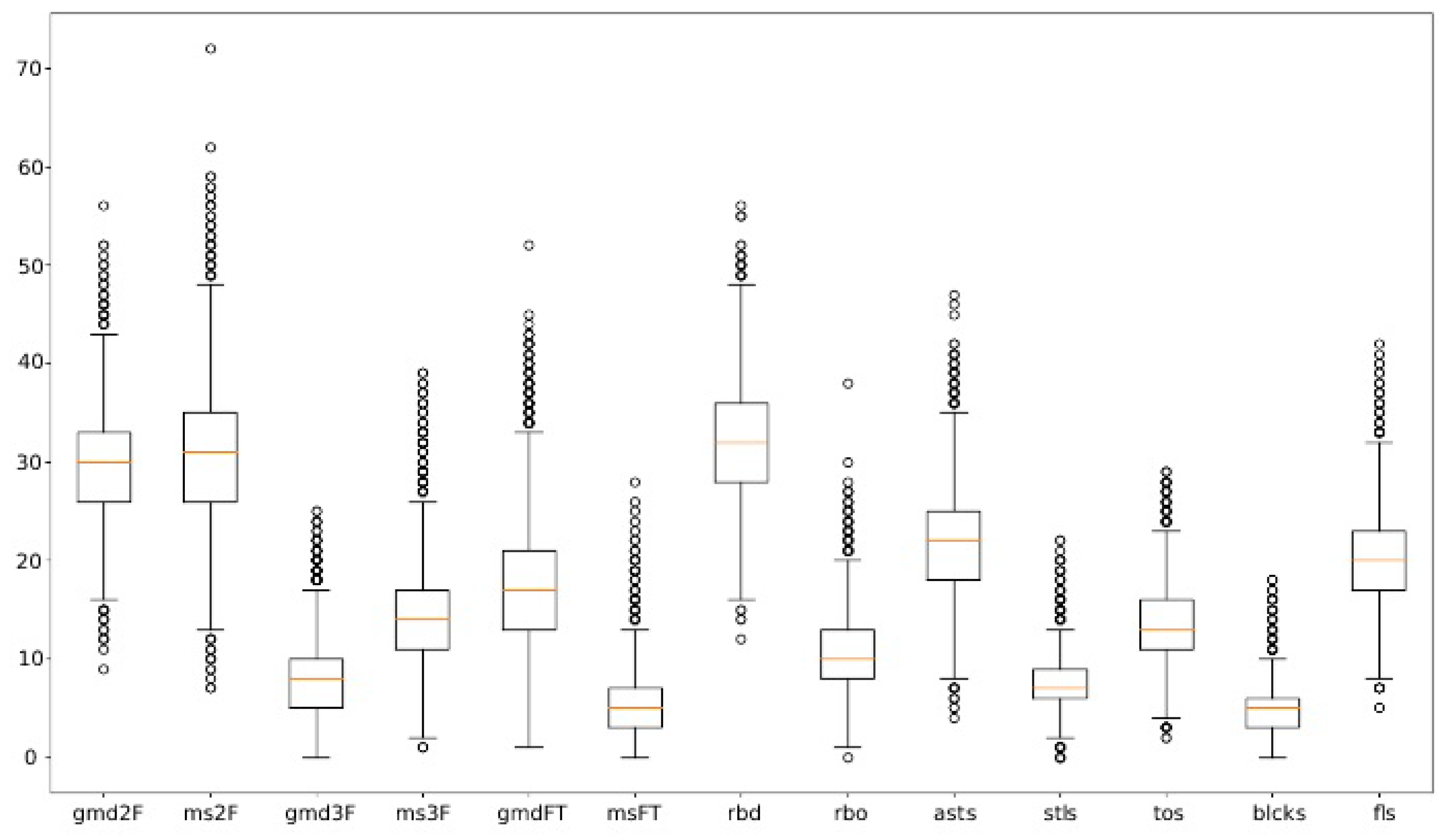
3.2. Data Preparation and Feature Extraction

Data preparation in ML includes proper feature extraction, which consists of feature engineering, feature selection, and if needed, dimensionality reduction. As for the feature engineering, we addressed it in Section 2, where we discussed the basic and advanced basketball elements and derived other indicators from them, such as the NBA team efficiency index. In the context of ML, all these indicators can be treated as features. From them, we manually select those features that will contribute most to the particular goal of the data analysis. In general, feature extraction is a process of reducing the dimensionality of the original, raw dataset into one that is more manageable for processing [33].

In this work, we pursued two main goals and, thus, two types of feature extraction. First, we wanted to determine how accurately the NBA team efficiency index reflects the outcome of a game on average. To accomplish that, we used the first set of features, consisting of thirteen basic game-specific elements listed in Table 1. These features were collected separately for each game so that we could verify how well the estimated ${\omega }_G^{\prime }$ outcomes based on the $I_{\mathrm{NBA}}$ matched the actual ${\omega }_G$ outcomes of those games. The same is then repeated with the reduced set of basic features, obtained by the feature selection based on the information gain calculated for those features with respect to the estimated outcome of all games $G_i$ played by both teams from the observed pair $(T{m}_1,T{m}_2)$. In this feature selection process, only the features that had information gain greater than the average information gain of all the features in the starting set remained in the reduced set. The final feature set was the union of the reduced feature sets for both teams. However, such a reduction spoiled the prediction accuracy significantly and turned out to be counterproductive. This is elaborated in Subsection 5.1 and can be inspected in Table 8. Because of that, we kept the integral set of basic features without applying dimensionality reduction. The statistical presentation of those features, collected from the observed NBA games belonging to the whole training set, are shown in the form of a box plot in Figure 1.

The second purpose of the data preparation was to determine the average team performance indicators from the training season dataset or the optimal time window and the league rating characteristics based on the entire training dataset. To do that, the features from the four sets of basketball game elements or data features were used in this work, in whole or partly: (1) the set of thirteen basic game elements, listed in Table 1; (2) the set containing eight derived game elements, given in Table 2; (3) the set of thirteen advanced game elements, suggested mostly by the NBA analyst and statistician Dean Oliver [34] presented here, in

Table 3. Thirteen advanced basketball game elements that constitute the advanced feature set.

Game el. / Feature Abbrev.	Description	Calculation Formula
gScsFld,  gScsFT	Field goal, and free throw success ratio	$r_{\mathrm{gScsFld}}=\frac{N_{\mathrm{gmdFld}}}{N_{\mathrm{gatFld}}},r_{\mathrm{gScsFT}}=\frac{N_{\mathrm{gmdFT}}}{N_{\mathrm{gatFT}}}$
gEffFld	Effective field goals (usually in %)	$r_{\mathrm{gEffFld}}=\frac{2\times N_{\text{gmd2F}}+3\times N_{\text{gmd3F}}}{2\times N_{\mathrm{gatFld}}}=\frac{N_{\mathrm{gmdFld}}+0.5\times N_{\text{gmd3F}}}{N_{\mathrm{gatFld}}}$
ScsTruSht	True shooting success ratio (usually in %).	$r_{\mathrm{ScsTruSht}}=\frac{N_{\mathrm{pts}}}{2\times (N_{\mathrm{gatFld}}+0.44\times N_{\mathrm{gatFT}})}$
gatFT/gatFld	Free throw attempt to field goal attempt ratio (free throw rate).	$r_{\text{gatFT/gatFld}}=\frac{N_{\mathrm{gatFT}}}{N_{\mathrm{gatFld}}}$
rbd/rbs,  rbo/rbs	Defensive and offensive rebound ratio	$r_{\text{rbd/rbs}}=\frac{N_{\mathrm{rbd}}}{N_{\mathrm{rbs}}},r_{\text{rbo/rbs}}=\frac{N_{\mathrm{rbo}}}{N_{\mathrm{rbs}}}$
asts/Pts	Ratio of the numbers of assists and total points	$r_{\text{asts/pts}}=\frac{N_{\mathrm{asts}}}{N_{\mathrm{pts}}}$
blcks/OppGatFld	Ratio showing the number of blocks per one opponent-team field goal attempt	$r_{\text{blcks/OppGatFld}}=\frac{N_{\mathrm{blcks}}}{N_{\mathrm{OppGatFld}}}$
poss	Number of ball possessions.	$N_{\mathrm{poss}}=0.96\times (N_{\mathrm{gatFld}}+0.44N_{\mathrm{gatFT}}+N_{\mathrm{tos}}-N_{\mathrm{rbo}})$
Offens%	Offensive rating (percentage)	$r_{\text{Offens\%}}=\frac{N_{\mathrm{pts}}}{N_{\mathrm{poss}}}/\times 100\%$
tos/poss%	Turnover to possessions percentage	$r_{\text{tos/poss\%}}=\frac{N_{\mathrm{tos}}}{N_{\mathrm{poss}}}\times 100\%$
GmScr	Hollinger’s Game Score	$N_{\mathrm{GmScr}}=N_{\mathrm{pts}}+0.4N_{\mathrm{gmdFld}}-0.7N_{\mathrm{gatFld}}-0.4(N_{\mathrm{gatFT}}-N_{\mathrm{gmdFT}})+N_{\mathrm{fls}}]+0.7[N_{\mathrm{rbo}}+N_{\mathrm{asts}}+N_{\mathrm{blcks}}]+0.3N_{\mathrm{rbd}}+N_{\mathrm{stls}}+N_{\mathrm{tos}}$

; and (4) the set consisting of eight league-wise team game elements, listed in

Table 4. Eight league-wise basketball game elements that constitute the league-standing feature set.

Game el. / Feature Abbrev.	Description	Label and Formula
WLR10LstGms	Win-loss record, i.e., the ratio (percentage) of the games won in the last 10 games.	$r_{\text{WLR10LstGms}}=N_{\text{gmsWn,10LstGms}}/10$
WLR10LG, HTHG	Win-loss record for a home team (HT) in (the last 10) home games (HG).	$r_{\text{WLR10LG,HTHG}}=N_{\text{gmsWn10LG,HTHG}}/10$
WLR10LG, GTGG	Win-loss record for a guest team (GT) in (the last 10) guest games (GG).	$r_{\text{WLR10LG,GTGG}}=N_{\text{gmsWn10LG,GTGG}}/10$
WLR10LG, HTMG	Win-loss record for a home team (HT) in (the last 10) mutual games (MG) with an opponent.	$r_{\text{WLR10LG,HTGG}}=N_{\text{gmsWn10,GTGG}}$
WLR, TstPer	Win-loss record in the testing period	$r_{\text{WLR,TstPer}}=N_{\text{gmsWn,TstPer}}/N_{\text{gmsTot,TstPer}}$
WnStrk	Winning streak = the number of games won in a row.	$N_{\mathrm{WnStrk}}\ge 0$
GmsIn10LstDys	Number of games in the last 10 days.	$N_{\text{GmsIn10LstDys}}$
RstDys	Number of the rest days (the whole days without playing any game) before some observed game.	$N_{\text{GmsIn,10LstDys}}\ge 0$

. In this approach, we simply considered all the stated features.

In general, the problem of missing or sparse values should be addressed before performing feature extraction. Since we worked with a relatively small and complete dataset, with about 6000 rows, this problem did not arise. If the problem does occur, one should fill in the missing data with generated replacement values, e.g., by using the k-nearest neighbors method. In a similar manner, we only crudely checked the full sets of exact data for possible outliers. Since there were no significant deviations in the data values, we did not perform any outlier elimination. Finally, for an efficient ML model, all input data must be normalized, by default to the fixed interval of 0 to 1.

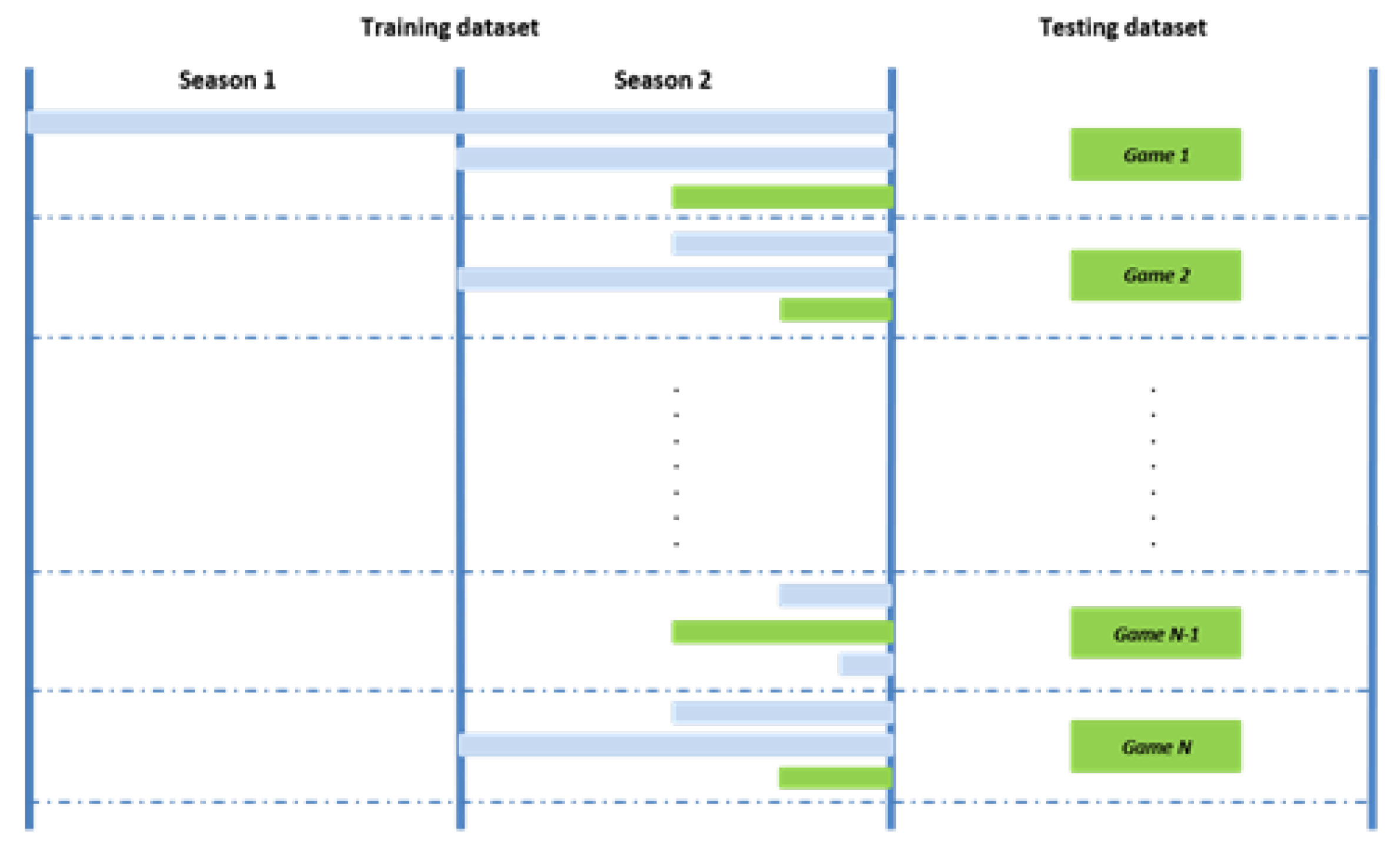
3.3. Optimal Time Window

In the proposed prediction model, we introduced the concept of optimal time window (OTW). It is the time window within the time span of the training data set, ${\mathcal{D}}_{\mathrm{tr}.}$. The (training) data from the OTW form the OTW dataset, ${\mathcal{D}}_{\mathrm{OTW}}$, which is a subset of ${\mathcal{D}}_{\mathrm{tr}.}$ (${\mathcal{D}}_{\mathrm{OTW}}\subseteq {\mathcal{D}}_{\mathrm{tr}.}$). Of course, ${\mathcal{D}}_{\mathrm{tr}.}$, and thus also ${\mathcal{D}}_{\mathrm{OTW}}$, are prior to ${\mathcal{D}}_{\mathrm{tst}.}$. Now we define ${\mathcal{D}}_{\mathrm{OTW}}$ as the subset of a training dataset that gives the highest correlation between the relative NBA team efficiency index (Equation (6) using the Equation (2) index) and the relative game score (Equation (7)) for the observed team. The OTW is the time range of data from ${\mathcal{D}}_{\mathrm{OTW}}$.

In other words, ${\mathcal{D}}_{\mathrm{OTW}}$ is the dataset from the past—determined by the OTW—that best describes the current state of the observed team regarding the achieved relative scores in the (near) future.

Each team has its own characteristics that can vary in the form of ups and downs, so it is crucial to find out that window. The OTW will be organized as a time period with a certain number of games, for which this number is divisible into equal or similar smaller numbers.

By defining the input feature sets, we will create the necessary conditions for our model, and by finding the OTW, we will ensure its optimal performance. At each new iteration of the model—i.e., at each new game of the observed team(s)—we update and extend the training dataset with a previous testing dataset and simultaneously define the new testing dataset from the most recent games. In this procedure, we keep the training and testing datasets mutually disjoint while ensuring the optimal history of system events.

Figure 2 illustrates the method for calculating the OTW based on the training and testing datasets. It is performed separately for each team at the time of prediction. The training dataset is divided into three subsets, all the potential OTWs: the entire training dataset, the second half of the training dataset, and the second half of the latter, i.e., the quarter of the training dataset. The entire training data set spans up to before the first game in the testing dataset for which the outcome is to be predicted. In each iteration, among the three data subsets, the optimal one is selected according to the above definition, that is, as the one that has the best correlation between the relative NBA team efficiency index and the relative score. Its time span is chosen as the current OTW. In each subsequent iteration, the previous OTW is used as the reference period for each analyzed team, and two other periods are defined: one half its size (if possible) and another double its size. When having N test games in a series, $G_1,G_2,\cdots ,G_N$, after finding the OTW for the game $G_1$, this game is transferred from the testing to the training dataset so that the OTW can be determined for $G_2$, etc., always keeping its size a constant number of games.

4. Prediction Model

In this section, we first briefly list the standard supervised learning algorithms that we have used for the prediction of the basketball game outcomes and present the results obtained by them (Subsection 4.1). Then, in the next subsection (Subsection 4.2), we outline our prediction model based on the usage of the predicted team efficiency index introduced in Subsection 2.5.

4.1. Predictions by the Standard Supervised Learning Algorithms

Here we outline the results of the game outcome predictions obtained by using the standard supervised learning algorithms, applied to the input data set that consists of the elements of the basic basketball game statistics (Table 1). The analysis was performed by using the Weka ML tool ([10], cf. also Subsection 1.2). One to three seasons of the training set and one to two seasons of the test set were used. For each ML algorithm stated,

Table 5. The use of standard ML classifiers and their prediction accuracy.

ML Classifier	Accuracy
Logistic Regression	56.1%
Naive Bayes	55.8%
Decision trees	53.5%
Multilayer perceptron	56.1%
K-nearest neighbours	57.9%
Random forest	56.3%
LogitBoost	54.5%
Average	55.8%

shows the representative results after combining the best-performing training and testing datasets from several seasons. Further details on the implementation and the results of this prediction go beyond the scope and volume of this paper.

To briefly conclude, the very low prediction accuracy—not much higher than pure guessing or flipping a coin—clearly shows that using either of the listed ML classifiers on the raw basketball statistics did not provide a good model for this purpose. This fact was a clear motivation to investigate different approaches and search for a better model.

4.2. The Proposed Prediction Model

Our prediction model uses all three different feature sets described in Subsection 3.2, summarized in Table 1, Table 2, Table 3 and Table 4. The prediction discrimination function in this model relies on the idea of the predicted team efficiency index and the quantities derived from it in Subsection 2.3, Subsection 2.4, Subsection 2.5 and Subsection 2.6. Mathematically speaking, our “measure” on the space of n-dimensional vectors, whose coordinates correspond to the observed team features of the basketball game, will be a simple linear combination of those coordinate values for each point (game) in that space, calculated as the NBA team efficiency index (Equation (5) with the NBA player efficiency index, from Equation (2)). Furthermore, since our goal is to predict the game outcomes, we will adapt the team efficiency index to not only record the achievements of the observed team but to additionally reward whenever it outperforms its rival in chosen game elements.

With the above idea in mind, we extend the basic team efficiency index—calculated, as in Equation (5), from only the contributions of the team players—with the part that compares the performances of the observed team to its opponent team in a game, for a set of chosen features. That is, in a game G, played by the pair of teams $(T{m}_1,T{m}_2)$, we introduce the extended$I_{\mathrm{EXT},Gm,T{m}_1\to T{m}_2}$ team efficiency index as follows:

$$I_{\mathrm{EXT},G_{T{m}_1\to T{m}_2}}=I_{\mathrm{BASIC},G_{T{m}_1}}+I_{\mathrm{CMPR},G_{T{m}_1\to T{m}_2}}.$$

(13a)

$I_{\mathrm{BASIC},Gm,T{m}_1}$ can be calculated from the set of basic features (Table 1), treating them separately or combining them in some kind of efficiency index. In our case, we have normally used the latter choice and used the NBA team efficiency index, so that

$$I_{\mathrm{BASIC},G_{T{m}_1}}=I_{\mathrm{NBA},G_{T{m}_1}}.$$

(13b)

The comparative part, $I_{\mathrm{CMPR},Gm,T{m}_1\to T{m}_2}$, is increased whenever $T{m}_1$ outperforms $T{m}_2$ in a positive game feature, and is decreased whenever it “outperforms”, i.e., has a greater number than the opponent, for a negative feature. These changes are defined by expressions in the last column of

Table 6. Calculation of $I_{\mathrm{CMPR}}$ for the set of selected basketball game elements (features). The last column specifies how $I_{\mathrm{CMPR}}$ changes when, in a certain game, the observed team outperforms its rival in each feature (cf. Table 1, Table 2, Table 3 and Table 4). In the case of a tie, $I_{\mathrm{CMPR}}$ stays unchanged. ‘−||−’ = the same as above.

Feature Set (Type)	Feature Abbrev.	Change of ${\mathit{I}}_{\mathbf{CMPR}}$
Basic (+)	asts, blcks	$I_{\mathrm{CMPR}}\leftarrow I_{\mathrm{CMPR}}+1$
Derived (+)	pts, rbs	–||–
Advanced (+)	gScsFld,  gScsFT,  gEffFld	$I_{\mathrm{CMPR}}\leftarrow I_{\mathrm{CMPR}}+1$
	ScsTruSht, gatFT/gatFld	–||–
	rbd/rbs, rbo/rbs	–||–
	asts/Pts, blcks/OppGatFld	–||–
	poss	–||–
	Offens%, tos/poss%	–||–
	GmScr	–||–
League standing (+)	WLR10LstGms	$I_{\mathrm{CMPR}}\leftarrow I_{\mathrm{CMPR}}+1$
	WLR10LG, HTMG	–||–
	WLR10LG, HTHG	–||–
	RstDys	–||–
	WLR, TstPer	–||–
	WnStrk	$I_{\mathrm{CMPR}}\leftarrow I_{\mathrm{CMPR}}+N_{\mathrm{WnStrk}}$
League standing (−)	GmsIn10LstDys	$I_{\mathrm{CMPR}}\leftarrow I_{\mathrm{CMPR}}-N_{\text{GmsIn10LstDys}}$

. There is just one negative feature there: GmsIn10LstDys, in the league standing set, and only for this feature, $I_{\mathrm{CMPR}}$ is decremented. If both teams have equal contributions, $I_{\mathrm{CMPR}}$ does not change.

Summarily, the preponderance of the observed team to its opponent is checked for the following: (i) two basic game elements, from Table 1, (ii) two derived game elements, from Table 2, (iii) all thirteen advanced game elements, from Table 3, and (iv) all eight league-wise game elements, from Table 4. A careful reader will note that the features from basic (asts, blcks) and derived (pts, rbs) sets of elements all appear as the corresponding numbers ($N_{\mathrm{asts}}$, $N_{\mathrm{asts}}$, $N_{\mathrm{pts}}$, $N_{\mathrm{rbs}}$) in the NBA team efficiency index (Equations (2) and (5)), which constitutes the $I_{\mathrm{BASIC}}$ part of the extended team efficiency index.

The overall choice of the features that are compared in $I_{\mathrm{CMPR}}$, is based on many probes made in this and in our previous works. It is also—similarly to the other steps in this model—based on the basketball experience and expertise of the first author of this paper.

After the above definitions, we can calculate the predicted extended team efficiency index by inserting the above $I_{\mathrm{EXT}}$ index into Equation (10a), wherefrom we obtain:

$$\begin{array}{c}\hfill {\widehat{I}}_{\mathrm{EXT},G_{n+k,T{m}_1}}=\frac{1}{n}\sum _{i=1}^n{I}_{\mathrm{EXT},G_{i,T{m}_1\to T{m}_j}},k\ge 1,\\ \hfill G\in \mathcal{G},T{m}_1,T{m}_j\in \mathcal{T}m,T{m}_j\ne T{m}_1.\end{array}$$

(14)

As stated in Subsection 2.5, most often we choose $k=1$, to calculate the score of the very next game of the observed $Tm=T{m}_1$ team against its opponent, which we assume to be $T{m}_2$. For this team, we also calculate ${\widehat{I}}_{\mathrm{EXT},G_{n+1},T{m}_2}$ following Equation (14).

Having calculated the above indices for both teams, we can evaluate their predicted relative extended team efficiency index, ${\widehat{i}}_{\mathrm{EXT},G_{n+1},T{m}_1/T{m}_2}$, according to Equation (11), and then predict the outcome of their $G_{n+1}$ game by using the following, specialized version of Equation (12):

$${\widehat{\omega }}_{G_{(T{m}_1,T{m}_2)}}=\left\{\begin{array}{cc}+1,\hfill & {\widehat{i}}_{\mathrm{EXT},G_{n+1,T{m}_1/T{m}_2}}\ge 1,T{m}_1\mathrm{wins};\hfill \\ -1,\hfill & {\widehat{i}}_{\mathrm{EXT},G_{n+1,T{m}_1/T{m}_2}}<1,T{m}_2\mathrm{wins}.\hfill \end{array}\right.$$

(15)

Now, from the ${\widehat{I}}_{\mathrm{EXT},G_{n+k}}$ indices for both teams in the game $G_{n+k}$, one can determine the probabilities of winning for each team from the pair $(T{m}_1,T{m}_2)$. For $T{m}_1$ (the home team), this probability is:

$$\begin{array}{cc}\hfill \mathbf{Pr}\left(T{m}_1\mathrm{wins}\mathrm{in}{G}_{n+k,(T{m}_1,T{m}_2)}\right)& =\mathbf{Pr}({\widehat{i}}_{\mathrm{EXT},G_{n+1}}\ge 1)\hfill \\ \hfill & =\frac{{\widehat{I}}_{\mathrm{EXT},G_{n+k,T{m}_1}}}{{\widehat{I}}_{\mathrm{EXT},G_{n+k,T{m}_1}}+{\widehat{I}}_{\mathrm{EXT},G_{n+k,T{m}_2}}}.\hfill \end{array}$$

(16)

For the rival (guest) team, the probability is the opposite. We did not analyze these probabilities here, leaving this for some possible future work.

When calculating the above indices, the $I_{\mathrm{BASIC}}$ part was determined from data in the OTW. The same is valid for the $I_{\mathrm{CMPR}}$ part with the basic, derived, and advanced features, while the remaining contributions, of the league-standing features, were always determined from the whole training set.

To justify favoring the home team in Equations (12) and (15), we have analyzed the win/lose record of the home teams in the observed seasons.

Table 7. Home team win/lose record for the five analyzed seasons.

Season (s)	Games Won / Games Lost	Percentage of Games Won
2013/2014	764/555	57.9%
2014/2015	755/556	57.6%
2015/2016	782/534	59.4%
2016/2017	763/546	58.3%
2017/2018	770/542	58.7%
All five seasons	3834/2733	58.4%

shows that home teams win in the prevailing number of games. This conclusion can also be applied to the special case of the games in which both teams have the same predicted extended team efficiency indices, i.e., with ${\widehat{i}}_{\mathrm{EXT},G_{n+1},T{m}_1/T{m}_2}=1$. As expected, the number of such games is relatively small—in our case, less than 0.3%— so we observed the win/lose record for all observed games. Alternatively, this could also be performed for only the games with equalized ${\widehat{I}}_{\mathrm{EXT}}$.

5. Results

After describing our prediction model in the previous subsection (Subsection 4.2), here we first confirm the relevance of using the NBA team efficiency index as the foundation of that model and then present its accuracy in predicting the NBA game outcomes.

5.1. Estimating the Relevance of the NBA Team Efficiency Index

When commenting on the possible feature selection in Subsection 3.2, we have stated that by analyzing data corresponding to the basic feature set, one can calculate the team $I_{G_{Tm}}$ indices for all the team pairs in the observed games. From them, their relative $i_{G_{T{m}_1/T{m}_2}}$ or $i_{G_{T{m}_2/T{m}_1}}$ team efficiency indices (Equation (6)) and the estimated ${\omega }_G^{\prime }$ outcomes follow (Equation (9)). The latter can be compared to the actual ${\omega }_G$ game outcomes in the following manner (cf. Equations (8)):

$${\omega }_{G_{(T{m}_1,T{m}_2)}}^{\prime }\left\{\begin{array}{c}=\hfill \\ \ne \hfill \end{array}\right\}{\omega }_{G_{(T{m}_1,T{m}_2)}},$$

(17)

If the relation between the two outcmes is equality.

Table 8. Accuracy of the estimated ${\omega }_G^{\prime }\left(I_{\mathrm{NBA}}\right)$ win function based on the ratio of the $I_{\mathrm{NBA}}$ indices of the opponent teams obtained from data containing: (i) the whole basic feature set (the results averaged for the stated seasons) and (ii) only the features remained after the feature selection based on information gain. The basketball seasons are marked by their first years; e.g., 2013–2015 represents the three seasons: 2013/2014, 2014/2015, 2015/2016.

Dataset		Accuracy of  ${\mathit{I}}_{\mathbf{NBA}}$-Based Estimated win Funct.
Training (${\mathcal{D}}_{\mathbf{tr}.}$)	Testing (${\mathcal{D}}_{\mathbf{tst}.}$)	(i) Whole Basic ftr. Set	(ii) Selctd. Featrs. Only
2013–2015	2016–2017	92.0%	79.5%
2014–2015	2016–2017		79.0%
2015	2016–2017		78.0%
2013–2016	2017	91.8%	78.0%
2014–2016	2017		80.6%
2015–2016	2017		79.1%
2016	2017		78.4%

gives the percentages of accurately estimated game outcomes in the observed seasons, determined by the estimated ${\omega }_G^{\prime }\left(I_{\mathrm{NBA}}\right)$ win function (Equation (9)) and the NBA relative team efficiency index (Equation (6)) based on the NBA team efficiency index (Equations (5) and (2), respectively). In the third column, there are accuracies of these estimations obtained by using the whole set of basic features (Table 1). One can see that the $I_{\mathrm{NBA}}$-based estimated win function gives correct results in about 92% of the analyzed cases, which is similar to the accuracy of 92.3% found in [35]. Taking into account the amount of analyzed data, this justifies the claim that the NBA team efficiency index is a very relevant indicator of the performance of basketball teams. In the fourth column of Table 8, the same accuracies are given for the reduced basic feature set, obtained after the feature selection described in Subsection 3.2. Obviously, the reduction of the feature set led to the “truncated” NBA team efficiency index, whose estimating ability significantly decreased compared to the complete version of the index.

Regarding the estimated ${\omega }_G^{\prime }$ win function based on the NBA team efficiency index, one should notice that if the NBA index consisted of only the points scored ($N_{\mathrm{pts}}$, Equation (1a)), this percentage would increase to 100%. However, the applied feature selection process never resulted in exactly this case. On the other hand, the idea of an efficiency index is to include additional game elements that should also make a significant contribution to the performance of the team as a whole and to the results of the games it plays. If these additional contributions are balanced and correlate well with a team’s effective performance, then the correlation between the relative indices ($i_G$) and the relative scores ($r_G$) will approach one. Moreover, our other work dealing with the construction of a more general player efficiency index shows that this correlation is also very high for the NBA efficiency index despite its relative simplicity. We have in preparation a paper with an analysis of the correlation of our CPE index (cf. the comment in Subsection 2.3) and other basketball player efficiency indices—including the NBA one—to the relative game score. Of course, it is the very simplicity of calculating this index that has made it so popular and that it led the NBA to proclaim it the official metric for player performance evaluation for over 30 years. All this together was the reason why we chose it to be the basis of our team efficiency index.

5.2. Results of the Game Outcome Predictions

By using our prediction model from Subsection 4.2, summarized in Equation (15), we have calculated outcomes of more than 2500 NBA games from the observed basketball seasons. This is done for all the games from the testing seasons given in Table 8 and

Table 9. Accuracies of the game outcome predictions based on the prediction model from Subsection 4.2, using the subsets from: (A) training dataset (${\mathcal{D}}_{\text{tr.−X}}$) and (B) optimal time window (${\mathcal{D}}_{\text{OTW.−X}}$), each with three options of X: (i) lst. 10 gms. = last 10 games for teams $T{m}_1$ and $T{m}_2$ before the observed game $G_{i,(T{m}_1,T{m}_2)}$, (ii) 2 nd half = the second half of the given dataset, (iii) whole = the whole dataset. The games from the testing set for which the prediction is tested move to the training set. The testing is performed for all games in the observed seasons.

Initial Dataset Seasons		Prediction Accuracy (Overall: $65.9\%\pm 3.0\%$)
Training	Testing	(A) With Training Dataset ($64.5\%\pm 1.5\%$)			(B) With Dataset from OTW ($67.4\%\pm 3.6\%$)
(${\mathcal{D}}_{\mathbf{tr}.}$)	(${\mathcal{D}}_{\mathbf{tst}.}$)	${\mathcal{D}}_{\mathbf{\text{tr.−lst. 10 gms.}}}$	${\mathcal{D}}_{\mathbf{\text{tr.−2nd half}}}$	${\mathcal{D}}_{\mathbf{\text{tr.−whole}}}$	${\mathcal{D}}_{\mathbf{\text{OTW−lst. 10 gms.}}}$	${\mathcal{D}}_{\mathbf{\text{OTW−2nd half}}}$	${\mathcal{D}}_{\mathbf{\text{OTW−whole}}}$
2013–2015	2016–2017	63.7%	65.1%	64.7%	63.8%	67.3%	67.6%
2014–2015	2016–2017	63.6%	66.1%	65.7%	63.6%	67.4%	68.0%
2015	2016–2017	63.8%	65.4%	67.2%	64.1%	66.3%	70.0%
2013–2016	2017	62.8%	62.8%	62.8%	63.5%	65.2%	65.2%
2014–2016	2017	63.1%	63.8%	63.8%	63.7%	68.7%	68.4%
2015–2016	2017	63.0%	63.9%	64.5%	64.4%	70.2%	70.9%
2016	2017	63.9%	66.3%	68.3%	65.9%	72.4%	77.9%
	By columns:	$63.4\%\pm 0.4\%$	$64.8\%\pm 1.3\%$	$65.3\%\pm 1.9\%$	$64.1\%\pm 0.8\%$	$68.2\%\pm 2.5\%$	$69.7\%\pm 4.0\%$

. From the numbers of games given in Table 7, one can find that there were 1309 (1312) games in the testing season 2016/2017 (2017/2018), which gives the total sum of 2621 games.

The accuracies of those predictions are summarized in Table 9 for the two types of training data: (A) data taken from the specified (sub)sets of the training set (${\mathcal{D}}_{\mathrm{tr}.}$), and (B) data taken from the (sub)sets of the OTW dataset (${\mathcal{D}}_{\mathrm{OTW}}$).

For both cases, the training (sub-)datasets were organized in three ways, as described in the table caption.

As it was already explained in Subsection 3.3, the basic training (sub-)datasets were continuously updated by the games from the testing set for which the outcomes were already predicted. For example, for the sub-dataset ${\mathcal{D}}_{\mathrm{tr}.-\mathrm{lst}.10\mathrm{gms}.}$ (the first subcolumn in case A), when the prediction was made for the first game from the testing ${\mathcal{D}}_{\mathrm{tr}.-\mathrm{lst}.10\mathrm{gms}.}$ dataset, all previous ten games were taken from the starting, or initial, training dataset. After the prediction is calculated for this game, it is included in the now appended training dataset, prolonged for one game. After that, the new prediction is calculated for the second game from the testing dataset, etc. The analogous procedure is applied to the other two versions of ${\mathcal{D}}_{\mathrm{tr}.}$ (sub)sets of case A. In the B case, the OTW’s dataset is updated by the already observed game, but the oldest game is removed from it so that the cardinality of ${\mathcal{D}}_{\mathrm{OTW}}$ stays invariant (cf. Subsection 3.3).

We have also considered the possibility of using data from the (sub-)datasets for only the previous games of the observed team played against the opponent team in the game for which the prediction is made. If there are not enough such games, one could combine the statistics of those games with the statistics of all other games of the observed team. See also Equation (10b) and the discussion at the end of Subsection 2.5).

From the presented results, we see that the overall accuracy of $66\%\pm 1.5\%$ is significantly better than the accuracies that we obtained by using the (separate) game element data and the standard ML methods (Subsection 4.1, Table 5). Furthermore, method B—which uses the data from the OTW only—is overall slightly better, ≈3%, than method A, which uses the whole training set. Analyzing that difference by separate columns, ${\mathcal{D}}_{\mathrm{OTW}-\mathrm{lst}.10\mathrm{gms}.}$ is better than ${\mathcal{D}}_{\mathrm{tr}.-\mathrm{lst}.10\mathrm{gms}.}$, but not significantly. The remaining two columns in B have their mean values ≳2$\mathrm{std}.\mathrm{dev}$ greater than those of the corresponding columns in A, coming to the edge of significant improvement.

However, their last two rows, for the training datasets from the seasons 2015/2016, 2016/2017, and 2016/2107, and testing datasets from the seasons 2017/2018 in both rows, show the best individual prediction accuracies, >70%. Among them, the absolute best is the accuracy of 77.9%, obtained by using datasets with a single training (2016/2017) and a single testing (2017/2018) season. This value is significantly higher than other accuracies in the same column, which all correspond to the larger training datasets from either two or three earlier basketball seasons. Though this is a plausible result, in agreement with our previous work [32] discussed in Subsection 3.1, it would be good to confirm it with the analysis of additional data.

When analyzing the results of differently organized datasets, we noticed that—as could be expected—the prediction accuracy for a future game $G_{n+k,(T{m}_1,T{m}_2)}$ of a pair of teams rises when having a training dataset with more of their earlier mutual games This was already commented on in the previous paragraph of this section. On the other hand, the number of these games is often rather small, and these games are often from the far past. We leave further discussion of this matter for some other possible paper.

6. Conclusions

In applying ML to the prediction of team sports results, it is important to fully comprehend the complexity of the system being analyzed and—on the other hand–to find out the right indicators that will successfully correlate the myriad of collected statistical data to the future performance of the observed teams. The task is further complicated by the fact that many basketball games end up with a difference of only a few points out of around one hundred points scored by each team. Even more, team players and sportspersons in general are not machines. Knowing their performance yesterday still does not guarantee that they will perform equally tomorrow. This means that the outcomes of sports events depend not only on the measurable but also on many unmeasurable factors. The latter ones are to be considered by human experts who will make (human) decisions based on them. On the other hand, in an ML approach like this one, one should insist on measurable factors to obtain as objective predictions as possible. Still, to be successful in that, the use of heuristics is inevitable. Finally, if such a prognosis is considerably better than pure guessing, it should help humans improve and strengthen their decisions.

In this work, we have shown that the abundant basketball statistics based on such measurable factors provide sufficient ground for a quantitative estimation of the performance of a basketball team in the past and a prediction of its performance in the (near) future. The introduced notion of the general team efficiency index, based on some player efficiency index—in our case the standard NBA one—proved to be a good foundation for our model (Section 2). The set of basic game elements from which it is calculated represents the set of basic features of our ML model. In addition, we have introduced the relative version of this index, as the ratio of the team efficiency indices of the opponent teams. On the basis of this ratio, we formalized the estimated win function. In 92% of the investigated games during the five observed NBA seasons, this function based on the NBA team efficiency index gives correct outcomes of the games, proving that this index is a relevant indicator in predicting the game outcomes. If the feature set was reduced, making the NBA efficiency index incomplete, the accuracy of the estimated win function significantly decreased, showing that the initial feature set should be kept integral (Subsection 3.2 and Subsection 5.1).

In our prediction model, besides the NBA team efficiency index ($I_{\mathrm{NBA},G_{T{m}_1}}$), which is calculated from the basic feature contributions of only the observed team ($T{m}_1$), we have also added the comparing part of the index ($I_{\mathrm{CMPR},G_{T{m}_1\to T{m}_2}}$), which rewards the observed team with extra points whenever it outperforms its rival ($T{m}_2$) in a given game, in any of the selected game elements (features) outlined in Table 6. That is, the second part accounts not for the absolute values of the features—like the first part does—but accounts for the superiority of the observed team over the opponent team. In that sense, it brings both a qualitative novelty and a kind of asymmetry into the proposed model. We have chosen those features and determined the rewarding points heuristically, relying on our long-standing experience in analyzing basketball statistics and the results obtained by applying the trial-and-error method. By adding the two components, we formed the extended team efficiency index ($I_{\mathrm{EXT},G_{T{m}_1\to T{m}_2}}$, Equation (13)). From it, its predicted version follows (${\widehat{I}}_{\mathrm{EXT},G_{n+k,T{m}_1}}$, Equation (14)). By calculating this also for the opponent team, we can calculate the relative version of this index and determine the predicted game score (${\widehat{\omega }}_{G(T{m}_1,T{m}_2)}$, Equation (15)).

The overall accuracy of the predicted outcomes of 66% is satisfactory. It is significantly better than the accuracy obtained by using the basic feature set and the standard ML methods (cf. Table 5 and Table 9). The usage of the optimal time window (OTW) contributed slightly to the accuracies of the predictions, but on average, not much more than a single or double standard deviation of the obtained results. The exception and, at the same time, our best result, with prediction accuracy of ≈78%, is achieved with only one training and one testing season and using the data from the whole OTW.

Comparing these results to those achieved by other authors (Subsection 1.2), we see that they are satisfactory and that their accuracy competes successfully against the accuracies of the top results of others, except for a few of the best of them.

Regarding the generality of this work, the principle of the predicting model described here and applied to the NBA league teams and games is readily applicable to other basketball leagues, too. Namely, the primary reason for making the predictions for the NBA game outcomes was the abundance and availability of the statistics for this world’s largest and most famous league.

Although numerous variations of the predicting model and data organization were already investigated in this work, there are still many possibilities for improvement. One of them is to investigate if OTW could be calculated better to contribute more to the prediction accuracy. The other is to explore what past games should be taken into consideration and how to treat scarce data in some cases (e.g., if considering only the previous mutual games of the observed team and its opponent in the given future game). Furthermore, there is also room for improvement in finding other and more appropriate player efficiency indices and in adjusting their element coefficients, as well as in finding the optimal rewarding points in the comparing part of the introduced extensive team efficiency index. Such qualitative and quantitative upgrades of the proposed data-driven predicting model should contribute to its enhanced accuracy.

References

1. Alpaydin, E. Introduction to Machine Learning; MIT Press: Cambridge, MA, USA, 2020. [Google Scholar]
2. Prasetio, D.; Harlili, D. Predicting football match results with logistic regression. In Proceedings of the 2016 International Conference On Advanced Informatics: Concepts, Theory And Application (ICAICTA), Penang, Malaysia, 16–19 August 2016; pp. 1–5. [Google Scholar] [CrossRef]
3. Delen, D.; Cogdell, D.; Kasap, N. A comparative analysis of data mining methods in predicting NCAA bowl outcomes. Int. J. Forecast. 2012, 28, 543. [Google Scholar]
4. Valero, C.S. Predicting Win-Loss outcomes in MLB regular season games – A comparative study using data mining methods. Int. J. Comput. Sci. Sport 2016, 15, 91–112. [Google Scholar] [CrossRef]
5. Elfrink, T. Predicting the Outcomes of MLB Games with a Machine Learning Approach; Vrije Universiteit Amsterdam: Amsterdam, The Netherlands, 2018. [Google Scholar]
6. Horvat, T.; Job, J. The use of machine learning in sport outcome prediction: A review. WIREs Data Min. Knowl. Discov. 2020, 10, e1380. Available online: https://onlinelibrary.wiley.com/doi/pdf/10.1002/widm.1380 (accessed on 19 January 2023). [CrossRef]
7. Loeffelholz, B.; Bednar, E.; Bauer, K.W. Predicting NBA games using neural networks. J. Quant. Anal. Sport. 2009, 5. [Google Scholar] [CrossRef]
8. Miljković, D.; Gajić, L.; Kovačević, A.; Konjović, Z. The use of data mining for basketball matches outcomes prediction. In Proceedings of the IEEE 8th International Symposium on Intelligent Systems and Informatics, Subotica, Serbia, 10–11 September 2010; pp. 309–312. [Google Scholar] [CrossRef]
9. Zdravevski, E.; Kulakov, A. System for Prediction of the Winner in a Sports Game. In Proceedings of the International Conference on ICT Innovations; Springer: Berlin/Heidelberg, Germany, 2009; pp. 55–63. [Google Scholar]
10. Weka 3: Machine Learning Software in Java. Available online: https://www.cs.waikato.ac.nz/ml/weka/ (accessed on 3 March 2022).
11. Kravanja, A. Napovedanje Zmagovalcev Košarkaških Tekem. Doctoral dissertation, Univerza v Ljubljani, Ljubljanatel, Slovenia, 2013. [Google Scholar]
12. Torres, R.A. Prediction of NBA Games Based on Machine Learning Methods; University of Wisconsin: Madison, WI, USA, 2013. [Google Scholar]
13. Lin, J.; Short, L.; Sundaresan, V. Predicting national basketball association winners. CS 229 FINAL PROJECT 2014, 1–5. [Google Scholar]
14. Tran, T. Predicting NBA Games with Matrix Factorization. Ph.D. Thesis, Massachusetts Institute of Technology, Cambridge, MA, USA, 2016. [Google Scholar]
15. Cheng, G.; Zhang, Z.; Kyebambe, M.N.; Kimbugwe, N. Predicting the outcome of NBA playoffs based on the maximum entropy principle. Entropy 2016, 18, 450. [Google Scholar] [CrossRef]
16. Avalon, G.; Balci, B.; Guzman, J. Various Machine Learning Approaches to Predicting NBA Score Margins, 2016. Final Project. 2016. [Google Scholar]
17. Pai, P.F.; ChangLiao, L.H.; Lin, K.P. Analyzing basketball games by a support vector machines with decision tree model. Neural Comput. Appl. 2017, 28, 4159–4167. [Google Scholar] [CrossRef]
18. Lam, M.W. One-match-ahead forecasting in two-team sports with stacked Bayesian regressions. J. Artif. Intell. Soft Comput. Res. 2018, 8, 159–171. [Google Scholar] [CrossRef]
19. Ganguly, S.; Frank, N. The problem with win probability. In Proceedings of the 2018 MIT Sloan Sports Analytics Conference, Boston, MA, USA, 23–24 February 2018. [Google Scholar]
20. Ivanković, Z.; Racković, M.; Markoski, B.; Radosav, D.; Ivković, M. Analysis of basketball games using neural networks. In Proceedings of the 2010 11th International Symposium on Computational Intelligence and Informatics (CINTI), IEEE, Budapest, Hungary, 18–20 November 2010; pp. 251–256. [Google Scholar]
21. Trawiński, K. A fuzzy classification system for prediction of the results of the basketball games. In Proceedings of the International Conference on Fuzzy Systems, IEEE, Yantai, China, 10–12 August 2010; pp. 1–7. [Google Scholar]
22. Zimmermann, A.; Moorthy, S.; Shi, Z. Predicting college basketball match outcomes using machine learning techniques: Some results and lessons learned. arXiv 2013, arXiv:1310.3607. [Google Scholar]
23. Horvat, T.; Job, J.; Medved, V. Prediction of Euroleague games based on supervised classification algorithm k-nearest neighbours. In Proceedings of the 6th International Congress on Support Sciences Research and Technology Support, Setubal, Portugal, 20–21 September 2018; Volume 20, p. 21. [Google Scholar]
24. Manley, M. Martin Manley’s Basketball Heaven; Doubleday Books: New York, NY, USA, 1989. [Google Scholar]
25. Grossberg, S. Nonlinear neural networks: Principles, mechanisms, and architectures. Neural Netw. 1988, 1, 17–61. [Google Scholar] [CrossRef]
26. Yu, L.; Liu, H. Efficient Feature Selection via Analysis of Relevance and Redundancy. J. Mach. Learn. Res. 2004, 5, 1205–1224. [Google Scholar]
27. Han, J.; Kamber, M. Data Mining: Concepts and Techniques, 2nd ed.; The Morgan Kaufmann Series in Data Management Systems; Elsevier: Amsterdam, The Netherlands; Morgan Kaufmann: Burlington, MA, USA; Boston: San Francisco, CA, USA: San Francisco, CA, USA, 2006. [Google Scholar]
28. Basketball Stats and History Statistics, Scores, and History for the NBA, ABA, WNBA, and Top European Competition. Available online: https://www.basketball-reference.com (accessed on 3 March 2022).
29. Horvat, T.; Havas, L.; Medved, V. Web Application for Support in Basketball Game Analysis. In Proceedings of the icSPORTS, Lisbon, Portugal, 15–17 November 2015; pp. 225–231. [Google Scholar]
30. Horvat, T.; Havas, L.; Srpak, D.; Medved, V. Data-driven Basketball Web Application for Support in Making Decisions. In Proceedings of the icSPORTS, Vienna, Austria, 20–21 September 2019; pp. 239–244. [Google Scholar]
31. Horvat, T.; Job, J. Importance of the training dataset length in basketball game outcome prediction by using naïve classification machine learning methods. Elektrotehniški Vestn. 2019, 86, 197–202. [Google Scholar]
32. Horvat, T.; Havaš, L.; Srpak, D. The impact of selecting a validation method in machine learning on predicting basketball game outcomes. Symmetry 2020, 12, 431. [Google Scholar] [CrossRef]
33. Zhang, G.P. Neural networks for classification: A survey. IEEE Trans. Syst. Man Cybern. Part C 2000, 30, 451–462. [Google Scholar] [CrossRef]
34. Dean Oliver. Available online: https://en.wikipedia.org/wiki/Dean_Oliver_(statistician) (accessed on 3 March 2022).
35. Horvat, T. An Adaptive Method for Predicting Sport Outcomes Based on the Efficiency Index and Optimal Time Window. Ph.D. Thesis, Faculty of Electrical Engineering, Computer Science and Information Technology, University of Osijek, Osijek, Croatia, 2020. [Google Scholar]
Figure 1. Data of the thirteen basic basketball elements from Table 1, presented in the box plot diagram with the whiskers based on the 1.5 IQR (interquartile range) value. For each presented feature, the lower (upper) line of the rectangular box presents the first (third) quartile, denoted as Q 1 ( Q 3 ) . Q 1 and Q 3 define the IQR, r I Q = Q 3 Q 1 , which is the height of the box. The lighter line within the box presents the second Q 2 quartile, or median. The lower (upper) whisker is 1.5 × r I Q below (above) Q 1 ( Q 3 ) or coincides with the minimal (maximal) value, whichever is greater (smaller). The values below and above whiskers are denoted by circles: the lowest (highest) of them being the minimal (maximal) feature value. We did not treat these values as outliers.
Symmetry 15 00798 g001
Figure 2. Illustration of the OTWs (Optimal Time Windows, in green) and their relation to the time intervals of the training data sets (in light blue), for N games of the observed team. For the first game, all previous (training) games are from the training set only. For the later, G i games, with i = 2 , 3 , , N , besides the games from the training set, the games from the testing set up to G i 1 form the OTW.
Symmetry 15 00798 g002