A Novel Row Index Mathematical Procedure for the Mitigation of PV Output Power Losses during Partial Shading Conditions

Abstract

Energy demand forecasted for the next several years has been bench marked due to the massive need for electrical energy. Solar power plants have earned a great marketplace position in recent years, but also face challenges in terms of power dissipation due to the frequent occurrence of shade. As a result, the per unit solar electricity price increases drastically. There is an immense need to ensure the maximum dependable power conversion efficiency of Photovoltaic (PV) systems by mitigating power output losses during partial shading conditions. The reconfiguration of PV arrays is a useful, effective, and promising approach in this context. Though several reconfiguration techniques have been developed in recent years, their applicability to real-time power plants is debatable due to the requirement of many physical relocations, long interconnecting ties, and complexity. This research work proposes a novel row index mathematical procedure followed by a technique in which the reconfiguration matrix indexes are filled with a unique number so that no row number repeats in the same row and column. Additionally, the proposed approach uses small number of switches that reduce the cost as well as the computational complexity. To strengthen the analysis, very recent techniques such as Sudoku, Total Cross Tied (TCT), Chess-Knight, and Particle Swarm Optimization (PSO) based reconfiguration are compared against five different shading patterns. It has been observed that approximately 68% power loss is mitigated in TCT configuration. It is worth noting that it results in higher PV output power than the existing latest reconfiguration techniques such as PSO, Chess-Knight, Sudoku, and others.

1. Introduction

Conventional energy resources are dwindling rapidly, along with rising environmental issues, which results in the high adoption rate of renewable energy resources to meet with the total energy demand due to advancements in power conversion technology and the decreasing cost of Photovoltaic cells [1]. Reliable and efficient electric power conversion becomes ambiguous due to partial shading, which reduces energy harnessing capability and efficiency [2]. Therefore, partial shading has received a lot of attention in recent years as it distorts the nature of PV characteristics.

The PV modules can be interconnected in either a series or parallel configuration, since the voltage sum of the individual array voltages in series connection makes for a larger output voltage. Similarly, series connection restricts the flow of current to a single module. For parallel connections, where the system current is the total of each module current, the system voltage is limited to the voltage of a single module. Furthermore, the variety of interconnection designs such as Series-Parallel (SP), Bridge Linked (BL), TCT and Honey Comb (HC) are used to meet high power demand [3]. Figure 1 shows the schematics of different interconnection schemes. Partial shading mainly occurs due to the shadows of trees, buildings, and clouds, bird’s droppings, and dust accumulation. Solar PV systems suffer power output loss not only as a result of shaded areas, but also from shadow intensity and physical positions within the array. As a major solution, bypass diodes (BPDs) in shunt across PV modules minimize the possibility of hotspots and shadowing by providing a path for the current to follow when an open circuit is created due to shade. Bypass diodes are not an optimum solution due to their limitations, such as multiple peaks in I–V and P–V curves due to non-uniform irradiance on PV arrays [4]. The highest peak point between these peak points is the global maximum power point (GMPP), and the remaining points are the local maximum power point (LMPP), which makes the maximum power point trackers unable to track the global maximum power point of the PV system [5]. The technique utilizing micro converters is also a complex technique for achieving a high energy efficiency of the PV array [6]. The creation of multiple peaks due to bypass diodes and the extra maintenance requirement in cases of multilevel inverters, taking into consideration the cost factors for micro converters, motivates researchers to propose PV array reconfiguration. Reconfiguration is the process of physically or electrically repositioning PV panels to mitigate power loss by irradiance equalization [7].

The most common reconfiguration techniques are electrical array reconfiguration (EAR) or dynamic, physical relocation/static (PAR), and hybrid physical–electrical reconfiguration. Modules are adjusted dynamically inside the PV array to maximize power output under partial shading conditions (PSCs). Relays, electrical switches, and manual switches are used in Electric Array Reconfiguration (EAR) techniques to disperse shades. Even though these approaches provide dynamic switching matrices, obtaining the finalized relocation matrix is a difficult task [8]. Furthermore, the optimization-based switching matrix is proposed in [9], which necessitates the use of modular level sensors and data gathering. Similarly, the flexible switching matrix technique and real-time techniques in [10,11] propose string level reconfiguration, which requires manual switching and some additional sensors; this can be problematic and less reliable. In addition, all existing techniques require costly reconfiguration schemes. Several techniques have been established in this context, such as Genetic Algorithm (GA), Particle Swarm Optimization (PSO) [12], and Harris Hawks Optimizer (HHO). Although these techniques are promising, their implementations to real-time PV arrays are limited due to the need for several power electronic elements and sensors. Furthermore, switching circuit failures might cause L-L faults inside the arrays [13].

To compensate for the mismatch string current in EAR reconfiguration schemes, physical reconfiguration techniques that maintain the permanent circuitry are proposed. In this context, several puzzle-based techniques are proposed in [14,15,16,17]. Major limitations of puzzle-based PAR procedures are:

• They are only applicable to symmetrical PV arrays, and require distant column relocations;
• They need initial estimations that fundamentally influence shade dispersion;
• Reconfiguration requires sub-arrays.

Comparable disadvantages are analyzed to modify skyscraper [18], the hybridized rendition of skyscraper, and Ken-Ken puzzle [19]. Dominance square (DS) [20], competence square (CS) [21], and zig-zag movement [22] propose a lot of substantial reconfiguration rules in contrast to puzzle-based PAR approaches. These techniques dislodge PV modules to far off segments, which makes the reconfiguration cycle unreasonable and complex. In addition, distant column movements require difficult interconnections. In order to solve the problem of extensive connections, numerical methods that only follow a segment-wise movement were introduced in [23]. A detailed analysis of already existing techniques is mentioned in Table 1. These techniques are effective for a small size PV array, but they also are probably going to fail to meet expectations when implemented on the large photovoltaic clusters.

The literature study sums up the research gaps as:

• EAR strategies are uneconomical, and faults are lenient;
• PAR methods are effective for symmetrical PV arrays and require far off segment migrations;
• Far off column movement irritates wiring intricacy and limits the practical utilization of PAR strategies;
• Smooth I–V and P–V curves are very much necessary for maximum power extraction, and in most cases are not found.

This research work proposes a novel optimal row index-based reconfiguration method that could be applied to all PV clusters regardless of the above-mentioned limitations. The proposed technique uses straightforward numerical guidelines to identify the short gap between segments that can be made by deploying reasonable numerical strategy. Subsequently, the idea is to relocate the PV modules in odd rows corner to corner in a successive way without modifying the separate segments. This technique is very simple, as compared to its parent technique used in [14]. Curiously, the figured-out relocation rule is indistinguishable from the mathematical rule based on the arithmetic sequence. This approach is guaranteed to reduce the arduous interconnections issue and extra design work, which makes it straightforward to reconfigure it within the current framework design. More importantly, the technique can be scaled to any PV size. Since the final configuration can be reached in three to five simple numerical steps, this makes the computational effort of the proposed technique small. The results achieved are evaluated fairly using the recently tested Chess-Knight movement technique [24], conventional TCT, Sudoku, and PSO. In addition to its key performance indicators, the technology is evaluated and checked against five different shade cases to critically examine its performance. The proposed reconfiguration algorithm is static because it reconfigures the PV system in the same pattern for all shading scenarios, which is termed static reconfiguration. For comparative analysis, we have evaluated the proposed approach against recently published static reconfiguration approaches such as “Chess Knight Technique”, along with three other reconfiguration schemes. Further contributions of the proposed approach are as follows:

• The proposed method requires a short time for the module removal procedure, without adjusting the underlying section areas;
• The proposed reconfiguration technique reconfigures PV array once, so it requires nxn switches. In our case, the number of switches was 81. Other techniques require more switches;
• The innate similarity to both balanced and unsymmetrical PV systems has been conceptualized;
• It is scalable and descendible;
• As it requires less computation and a smaller number of switches, it is cost effective.

Table 1. Detailed review of existing techniques in the literature.

Sr. No	Techniques	Contributions	Limitations	Ref.
1	Sudoku Puzzle	Suitable for large dimensions	Not suitable for small size PV arrays Mathematical formulation is complex	[1]
2	Genetic Algorithm	Computationally effective	Large computational steps Poor convergence	[3]
3	Matrix Switching	Provides dynamic switching matrices	Implemented on small PV array sizes. Finding the final relocation matrix is a difficult task	[9]
4	Particle Swarm Optimization	Computationally effective Improves output power	Low convergence rate in iterative process	[12]
5	Futoshiki Puzzle	Improves output power	Complexity in connections	[14]
6	Magic Square	Difference between max value of sum of irradiances (SIR) and min value of SIR is low	Suitable for small size PV arrays only Only performs column scattering	[15]
7	Competence Square and Dominance Square	Applicable to large dimensions	Complex connections	[20,21]
8	Zig Zag Scheme	Electrical connections remain intact	Suitable for small size PV arrays Costly Complex connections	[22]
9	Improved Sudoku	Reduces mismatch compared to simple and optimized Sudoku	Effectiveness of technique is applicable to defined shading patterns	[25]
10	Optimal Sudoku	Reduced wiring	A lot of mathematical formulation	[26]
11	Fuzzy Logic	Suitable for different sizes	Determining radiation is a complex task	[27]
12	Shading Analysis using Image Processing	Reduces effect of partial shading Improves output power	Complexity in obtaining voltage and current at output	[28]

Table 1. Detailed review of existing techniques in the literature.

Sr. No	Techniques	Contributions	Limitations	Ref.
1	Sudoku Puzzle	Suitable for large dimensions	Not suitable for small size PV arrays Mathematical formulation is complex	[1]
2	Genetic Algorithm	Computationally effective	Large computational steps Poor convergence	[3]
3	Matrix Switching	Provides dynamic switching matrices	Implemented on small PV array sizes. Finding the final relocation matrix is a difficult task	[9]
4	Particle Swarm Optimization	Computationally effective Improves output power	Low convergence rate in iterative process	[12]
5	Futoshiki Puzzle	Improves output power	Complexity in connections	[14]
6	Magic Square	Difference between max value of sum of irradiances (SIR) and min value of SIR is low	Suitable for small size PV arrays only Only performs column scattering	[15]
7	Competence Square and Dominance Square	Applicable to large dimensions	Complex connections	[20,21]
8	Zig Zag Scheme	Electrical connections remain intact	Suitable for small size PV arrays Costly Complex connections	[22]
9	Improved Sudoku	Reduces mismatch compared to simple and optimized Sudoku	Effectiveness of technique is applicable to defined shading patterns	[25]
10	Optimal Sudoku	Reduced wiring	A lot of mathematical formulation	[26]
11	Fuzzy Logic	Suitable for different sizes	Determining radiation is a complex task	[27]
12	Shading Analysis using Image Processing	Reduces effect of partial shading Improves output power	Complexity in obtaining voltage and current at output	[28]

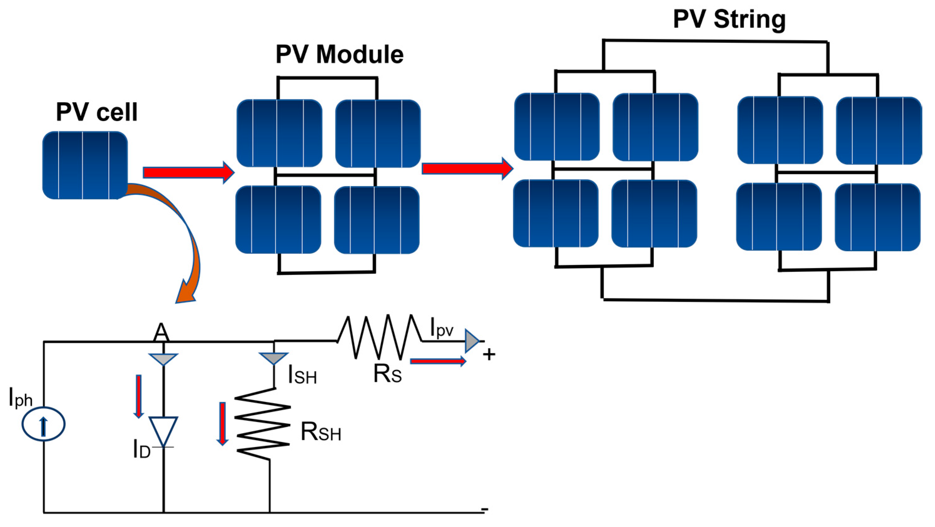
2. PV System Modeling

Different PV cell models, such as a single diode model, two diode model, and three diode model [29,30], have been proposed in the literature to assess the effectiveness of PV cells. Solar cells interconnect in series to form a module, and several modules combine to make a PV array. The single diode model of a solar cell is widely used due to simplicity. The equations below explain the working principle of the solar cell and PV array. As PV cells make the module and modules in parallel makes string, a parallel string makes the PV array, as in Figure 2.

KCL (Kirchhoff’s Current Law) can be applied to calculate the output current of the PV cell at node ‘A’, i.e., Equation (1) as in [31].

$$I_{pv}=I_{ph}-I_{D }-I_{SH}$$

(1)

$I_{ph}$ represents light generated current, $I_D$ represents diode current, and $I_{sh}$ is the shunt current. The right-side quantities are shown in Equations (2)–(4), as in [31,32].

$$I_{ph }=\frac{G}{Go} \ast \left[I_{sc}+K_i \left(T- T_o\right)\right]$$

(2)

$$I_D=I_o ⟦exp\left(\frac{q\left(V+R_s{I}_{pv}\right)}{\alpha kT}\right)-1⟧$$

(3)

$$I_{SH}=\frac{V+R_s{I}_{pv}}{R_{SH}}$$

(4)

G represents the current irradiance and Go is the irradiance at the standard test conditions; ($G_o$ = 1000 $\mathrm{W}/{\mathrm{m}}^2$), $Ki$ is the current temperature coefficient, $T$ is actual systems temperature, $To$ is the temperature at the STC; $To$ = (25 °C) [33], $I_o$ is the diode saturation current, $V$ is the output voltage, $R_s$ represents series resistance, $\alpha$ is the diodes ideality factor, $k$ is the Boltzmann constant, $q$ is the charge of an electron, and $R_{SH}$ represents shunt resistance.

After analyzing, Equation (1) becomes as that shown in Equation (5).

$$I_{pv }=\frac{G}{Go} \ast \left[I_{sc}+K_i \left(T- T_o\right)\right]-I_o ⟦exp\left(\frac{q\left(V+R_s{I}_{pv}\right)}{\alpha kT}\right)-1⟧-\frac{V+R_s{I}_{pv}}{R_{SH}}$$

(5)

Moreover, the photovoltaic array’s current relies upon the values of resulting string currents, which in this manner are subject to the ways in which the strings are associated. For the conventional instance of series/parallel electrical interconnections between various PV strings, the PV array current can be determined by Equation (6) as in [34].

$$I_{array}=N_p{I}_{ph}-N_p{I}_o\left\{⟦exp\left(\frac{q\left(V+R_s{I}_{pv}\right)}{\alpha N_s{V}_T}\right)-1⟧\right\}-\frac{1}{R_{SH}} \left[\frac{N_p}{N_s}V+R_{s}I\right]$$

(6)

The number of modules connected in series and parallel are denoted by $Ns$ and $Np$, respectively, and $V_T$ is the thermal voltage.

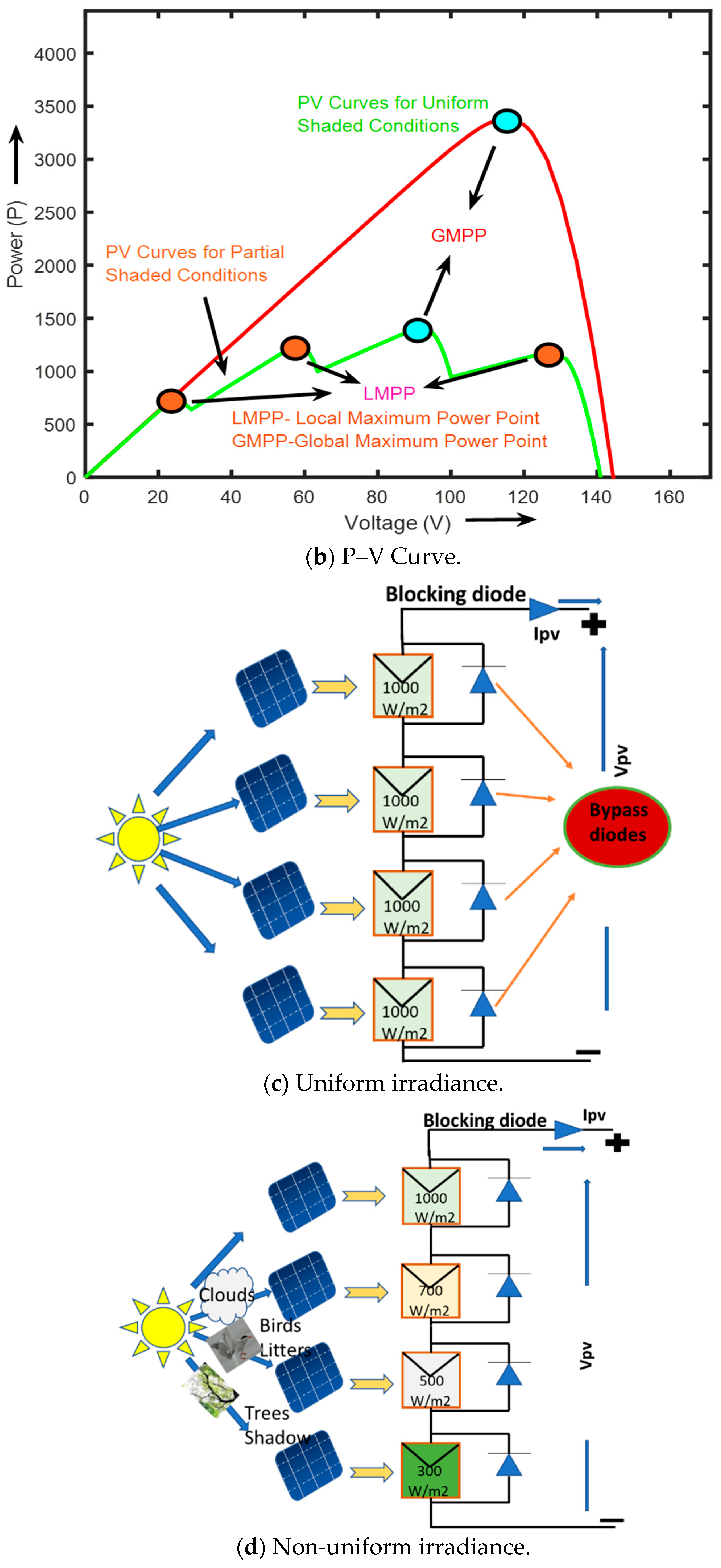
3. Effects of Partial Shading on the PV System’s Performance

In a string, a single shaded cell can decrease the current flowing through the unshaded cells in [35]. Despite using bypass diodes, several peaks appears in the P-V characteristic curve, as shown in Figure 3a,b and as in [36]. This characteristic presents a challenge to MPPTs since it forces such trackers to pick out a global peak amid several local peaks. This, in turn, increases the complexity of the MPPT design, which would have an economic impact on the design of the PV system. Figure 3c,d represent the causes of shading, and Figure 3e shows the overview of mitigation techniques with their effects.

Similarly, a kind of power loss known as an electric mismatch [37], occurs when photovoltaic modules with different current–voltage characteristics are coupled in series, as well as in parallel networks or arrays. The “mismatch loss” impact occurs when the total power output of the individual modules is greater than the overall power output of the PV array. The smooth I–V and P–V curves guarantees minimum variations in the row current. Characteristics curves with multiple peaks and several local minima(s) and maxima(s) result in mismatch fault. Our proposed algorithm not only mitigates power losses, but also reduces the mismatch fault by uniformly dispersing shading footprints and ensuring minimal divergence among the row current. Proposed reallocation is optimal. Figure 4 shows the classification of mismatch faults.

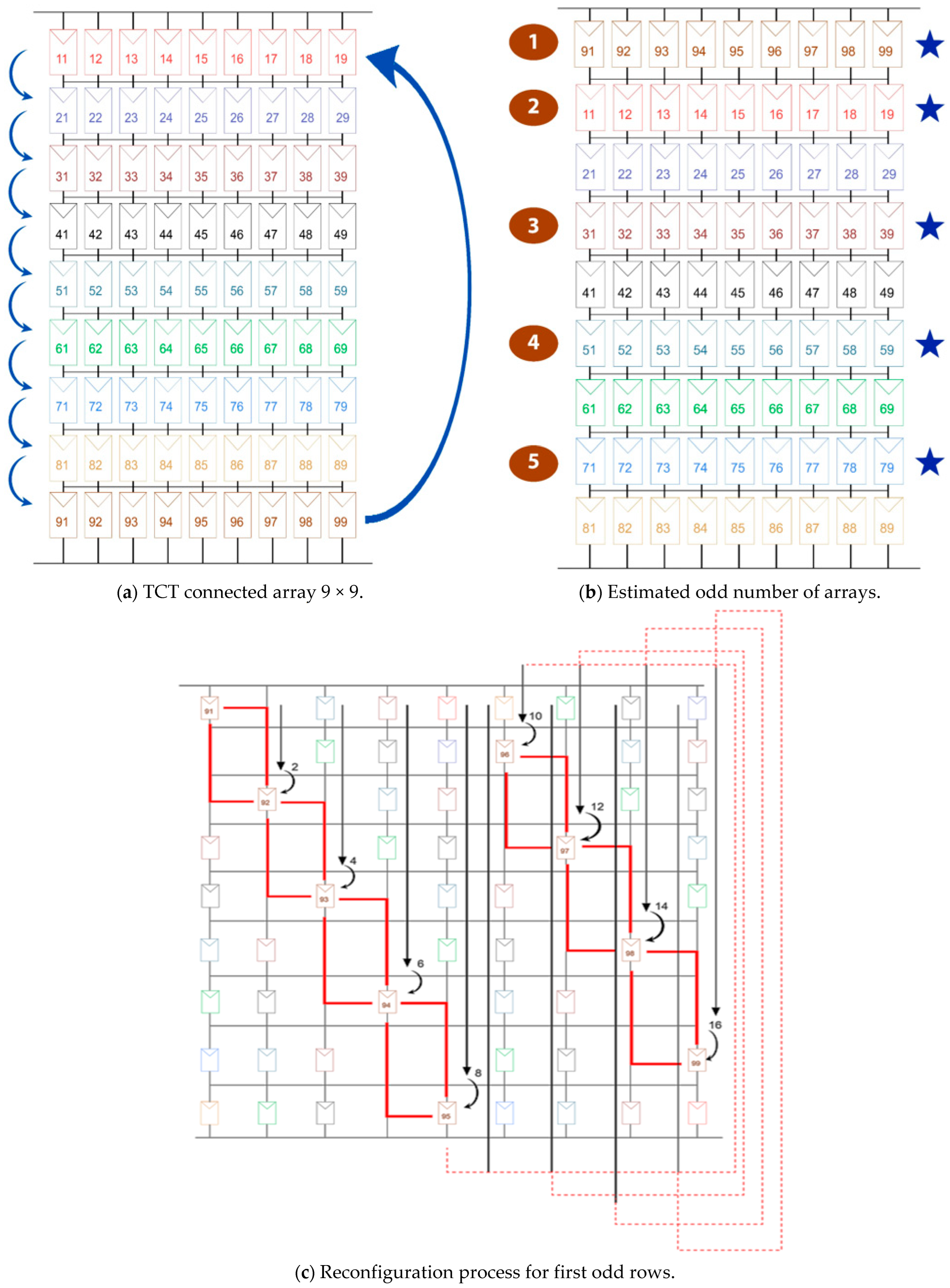
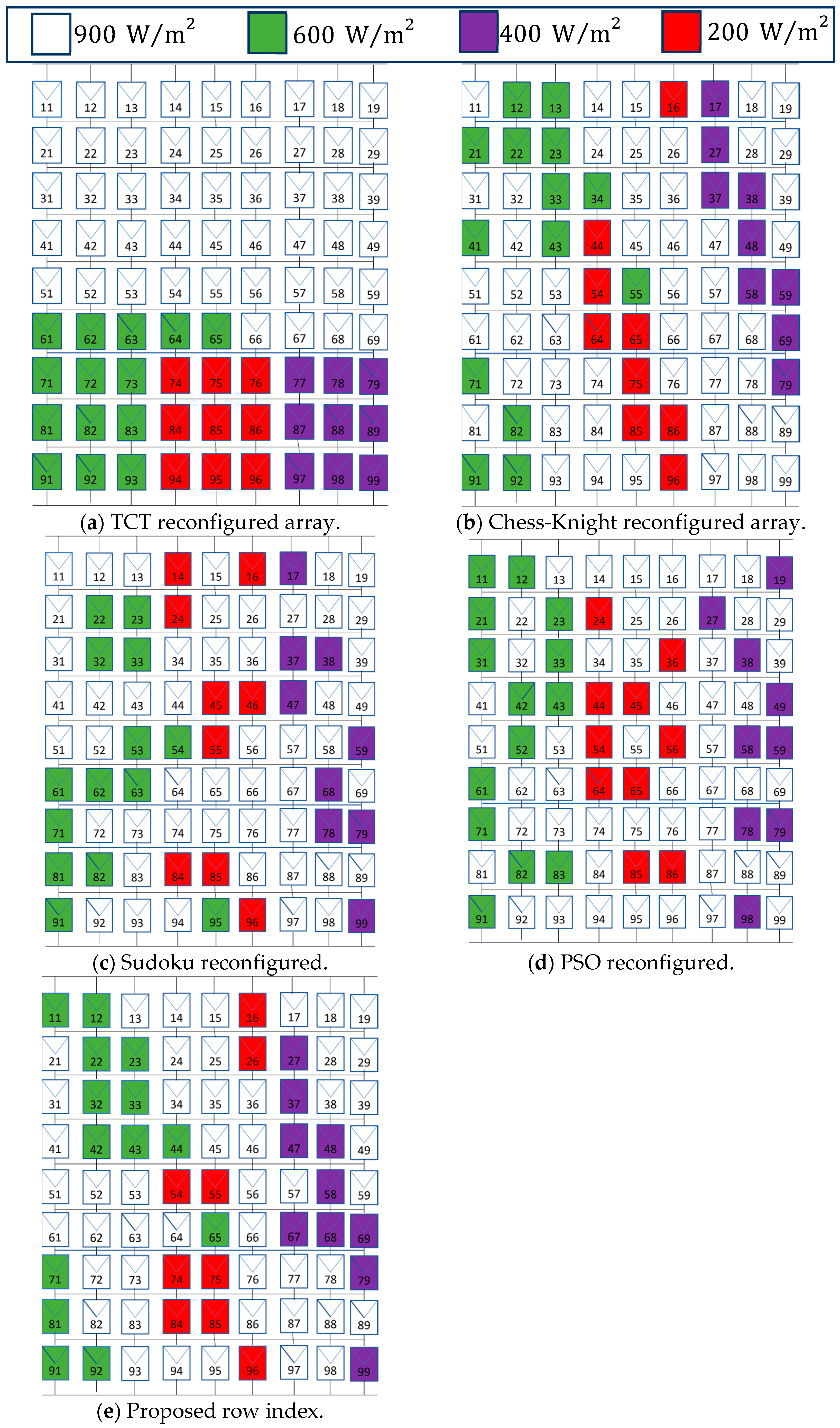
4. Array Reconfiguration with Total Cross Tied (TCT) Interconnection

A PV array under partial shadow conditions is taken into consideration to illustrate the requirement of array reconfiguration. Figure 5 shows the appropriate properties. Shade produces several power peaks [38], as can be seen. An example 5 × 5 TCT connector architecture with a specific shading pattern is displayed in Figure 5a to illustrate the array reconfiguration procedure. These are the intensities of shadows in each row of the chosen shade pattern. For both local and global contexts the P–V characteristic experiences peak because of the presence of shadow, as seen in Figure 5b,c, which show how array reconfiguration optimizes the placement of the shadowed PV panels and distributes the shade uniformly throughout the array. Additionally, it is clear from Figure 5d that a significant power gain of up to 887.68 W (3695.69 W compared to the previous 2808.01 W) is achieved. There are no longer any multiple peaks in the reconfigured structure. Thus, PV array reconfiguration provides a quick, reliable, and efficient method for reducing the impacts of shadow on a PV array.

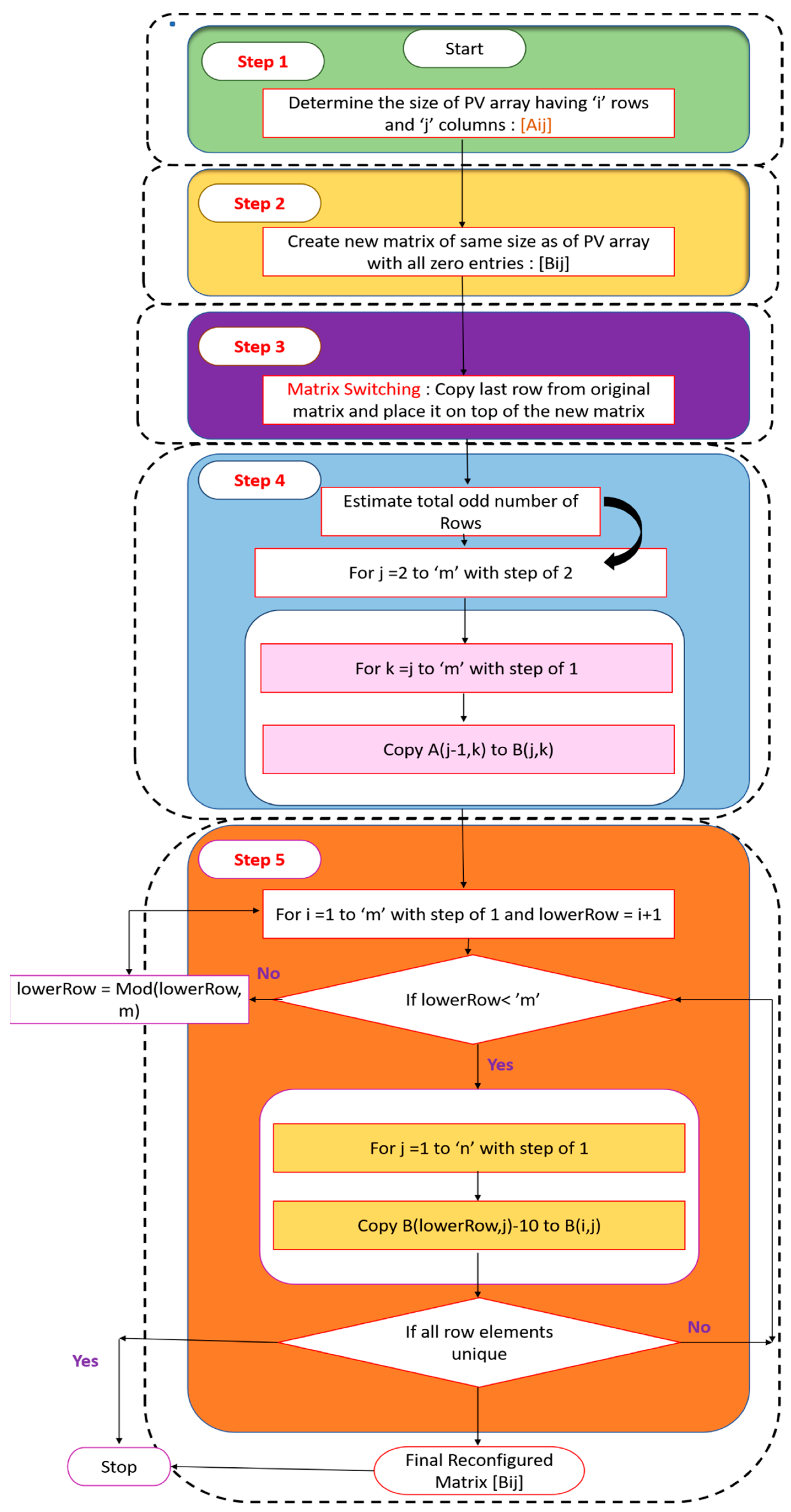
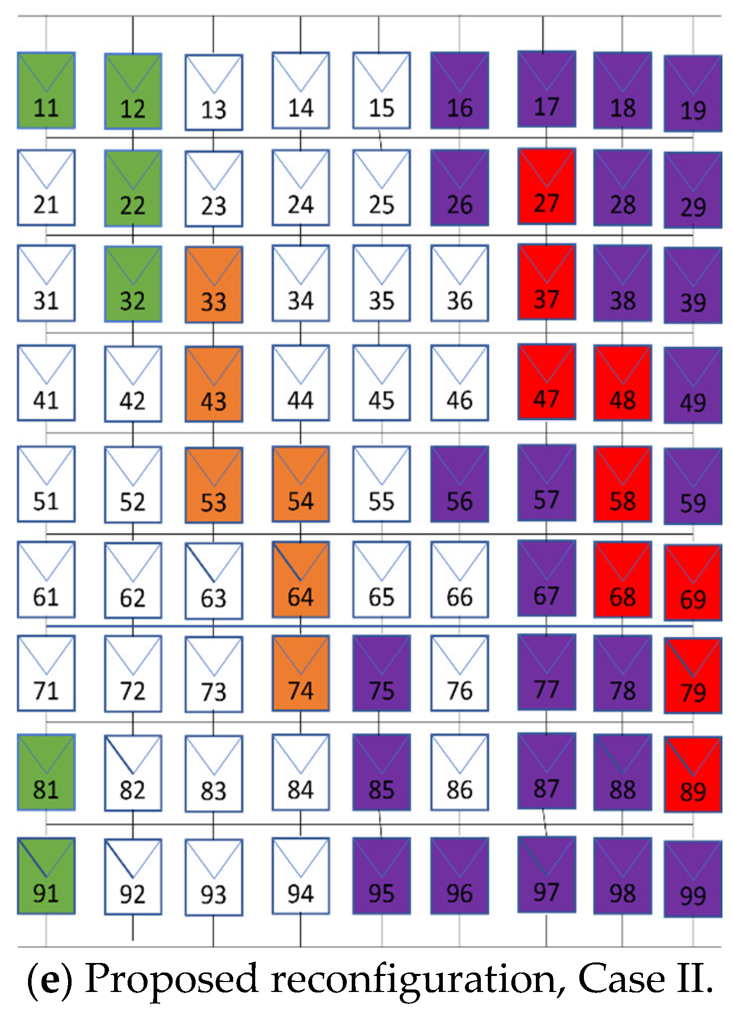
5. Proposed Methodology

This research work proposes a novel row indexed mathematical procedure that can be applied to any size of PV array. By considering each PV array as a square or non-square mathematical matrix, the suggested technique aims to reconfigure any PV array. This technique tries to move the components in each matrix column to other rows, but within the same column to achieve appropriate shadow dispersion. A specific row index based number relocation procedure followed the concept of a Futoshiki puzzle pattern [14]. This goal is accomplished because the remaining entries of each row which are not placed by the relocation procedure will be placed by each unique row number, such that no two row indexes have the same in each row. For the analysis of the test shade cases, we take the 9 × 9 PV array as an example. By using existing methodologies in the literature, it is possible to distinguish and compare the increased power production in different PSCs by choosing a larger PV array [16].

A row-index based proposed approach rearranges the PV panels, which are TCT connected. The PV panels which were originally placed in their initial position are relocated to the new position within the same column by following mathematical procedures, which are based on matrix shifting and the arithmetic sequence in initial and remaining odd row elements. They simply follow the blocks movement of the first negative row, and make their placements according to that. This relocation procedure is examined carefully, such that it can disperse the shade efficiently and effectively to obtain better output power in all unique shade patterns.

The proposed algorithm takes output power as an initial input, then reconfigures the system to mitigate power losses. The proposed algorithm has considered the five most common shading patterns, which are suggested in several recently published articles, and optimally reconfigures the PV system so that computational time and complexity are reduced. Additionally, this approach is a sensor-less approach; it takes output readings from inverters’ meters. Collecting the irradiance from each panel makes the system more complex and costly. Installing sensors on each panel also reduces the adoptability of the reconfiguration algorithm.

The 9 × 9 PV array matrix of 8.1 kW is designed. Variables ‘$i$’, ‘$j$’ and ‘$k$’ are used to identify the position of PV panels. At the start, the variable ‘$i$’ specifically represents row and ‘$j$’ represents the column in which each element is located initially. Therefore, ‘$ij$’ represents the position index of each element in the PV array; for example, ‘23′ means row number 2 and column number 3, as ‘$i$’ belongs to 2 and ‘$j$’ belongs to 3. That indicates that the PV module is positioned in the second row and first column in the array. The proposed method is given a name row index because at the first step all rows are shifted one step downward, and after that PV modules in the odd number of rows are placed in other rows but remain in the same column, followed by the unique method of filling remaining spaces in each row. To illustrate the row index based physical relocation technique, a simple 9 × 9 PV array is constructed and the sequential steps that are followed to reach at the final reconfigured matrix are explained below.

Step 1 to Step 3:

Determining the size of the PV array is the beginning of the methodology. Let us begin with a 9 × 9 PV array, with ‘$i$’ rows and ‘$j$’ columns. Consider the 9 × 9 PV array as a 9 × 9 matrix denoted by ‘$\left[Aij\right]$’, with a new matrix of the same size with all entries remain zero. Copy the last row of the first matrix and place it at the top of the new matrix. This is simply matrix shifting, and simply followed by shifting the first row to the second row, the second row to the third row, and continuing in the same way until all rows are placed in the same manner. The creation of a new matrix is not necessary, but was undertaken to give a detailed explanation of the procedure. This step’s use is easily visualized in Figure 6a.

Step 4:

Odd numbers of rows are estimated and marked before applying the mathematical concept, with the sign as shown in Figure 6b. This marking is necessary as only odd numbers of rows will follow mathematical procedure. For instance, the first entry of each row will not relocate, and its position will remain intact.

6. Proposed Arithmetic Sequence

This process repositions each entry except the first entry of odd numbers of rows to a new row, but within the same column by just following 2, 4, 6, 8, 10 and the onward sequence. The new position of each panel will be two rows downward from the prior panel position, but within the same column. For instance, we take the negative row entry where the panel is placed as ‘92’: now, the panel is placed in its new position based on the first entry of the arithmetic sequence, which is 2. The panel will move two steps downward and will be placed in a position one step downward from where it stops first. Hence, in this case the panel is shifted three places down by adding one position to where it fulfills the arithmetic sequence. Similarly, a panel at position ‘93′ will follow the next entry of the arithmetic sequence, which is 4, and be placed five places down, but you can see that it is two places down from the prior panel position but within the same column. After the completion of the arithmetic sequence rule by the first negative row, the remaining odd rows simply follow the placement of the first odd row panels and make their position according to that, by starting from their initial column position and relocating at the position where arithmetic sequence ends with one row downward. In this way, each entry of the odd number of rows will follow the same technique and will be placed in their new position. Figure 6c shows that each entry is just making a Straight L and inverted L path to indicate the new position of the next panel of the same row. That is also a way to achieve a new position, and fits in well with this technique.

Step 5:

In this step we will relocate the remaining panels that are not placed by arithmetic sequence, as shown in Figure 6d. This has an interesting procedure, keeping in view that row indexes must not repeat in vacant positions, with each other as well as with the already filled positions.

Relocation of Remaining Panels:

When all the panels of negative rows are placed successfully, panels of rows that are not relocated will be placed in their new position. After following the arithmetic sequence, each row has left some positions vacant where we will place other panels from the even numbers of rows. For example, the first odd row, which starts from the ‘9’ index row number, has four vacant positions, as seen in Figure 6d. We will simply make a rule here; in vacant positions, each panel must have a unique row index number, which is also a concept followed in the Futoshiki puzzle pattern. In that case, what panels come to the vacant positions of each row? In the first row there are four vacant positions, so keeping in mind that the row index must not repeat in the same row, and keeping the Futoshiki puzzle in mind, we can simply look at the panel position, which is one step downward from the vacant position, and choose a number in which adding one will make the row index that is already placed one step downward. An explanation is given as:

Vacant position column index number = 6

Vacant position row index number = x

Panel already placed below it has row index number = y = 9

Therefore, to place a panel in a vacant position: x + 1 = y

Vacant position (panel) row index would be = x = 8

Therefore, panel number ‘86′ will be placed above panel number ‘96′, and following this concept all the panels will be placed in each row, given the name row index method as shown in Figure 6e.

Figure 6f depicts the final PV array configuration following the proposed row index reconfiguration process. The moving technique in this reconfiguration design is easy, as is the wiring architecture, which also avoids the need for time-consuming interconnection links. This method of connection in the proposed approach is less expensive and will undoubtedly remain effective for all sorts of shadow events.

7. Generalized Proposed Concept

The proposed scheme can be used for any matrix of ‘$m$’ number of rows and ‘$n$’ number of columns. As a result, the method for converting the real matrix to a final reconfigure matrix are listed below.

Step 1: Determine the size of the input matrix [$A_{ij}$] as ‘$m\times n$’, ‘$i$’ varies from 1 to ‘$m$’ and ‘$j$’ varies from 1 to ‘$n$’;

Step 2: Initially create a new matrix of the same size, with all zero entries as B = zeros (size ([$A_{ij}$])), which in the end will merge with the original matrix [$A_{ij}$];

Step 3: Copy the last row from the original matrix and place it on the top of new matrix represented as: $b_{l\left(1,n\right)}=a_{m\left(1,n\right)}$;

Step 4: After matrix shifting, estimate the odd number of rows by applying arithmetic sequence on these rows, with a step of two represented as: $b_{\left(l,k\right)}=a_{\left(j-1,k\right)}$;

Step 5: It is to be considered each time that the row index should not repeat in the same row, and having the Futoshiki puzzle in mind just look at the panel position one step downward from the empty position and pick a number in which adding one will make the row index that is already set one step downward represented as: $b_{\left(i,j\right)}=b_{\left(lowerRow,j\right)}-10$. These are the generalized steps, and the flow chart is shown in Figure 7.

An important and interesting explanation regarding the utilizing of irradiation level/short circuit current or any other related parameter is that the output power is taken as an initializing parameter. In the TCT configured PV array, the percentage of shadow footprint to total PV area can be assumed by percentage reduction in the output power due to the fact that the TCT systems behave linearly to the shadow footprint, whereas in SP or configurations other than TCT different shadow footprints have different impacts due to series and parallel connections. In the series connected PV module, the power is reduced by 83% when only 10% of the module area comes under shadow. In TCT, the shadow footprint has a linear impact as it makes system LTI. Moreover, installing a pyranometer for checking and sensing irradiance at every module makes the system costly and complex.

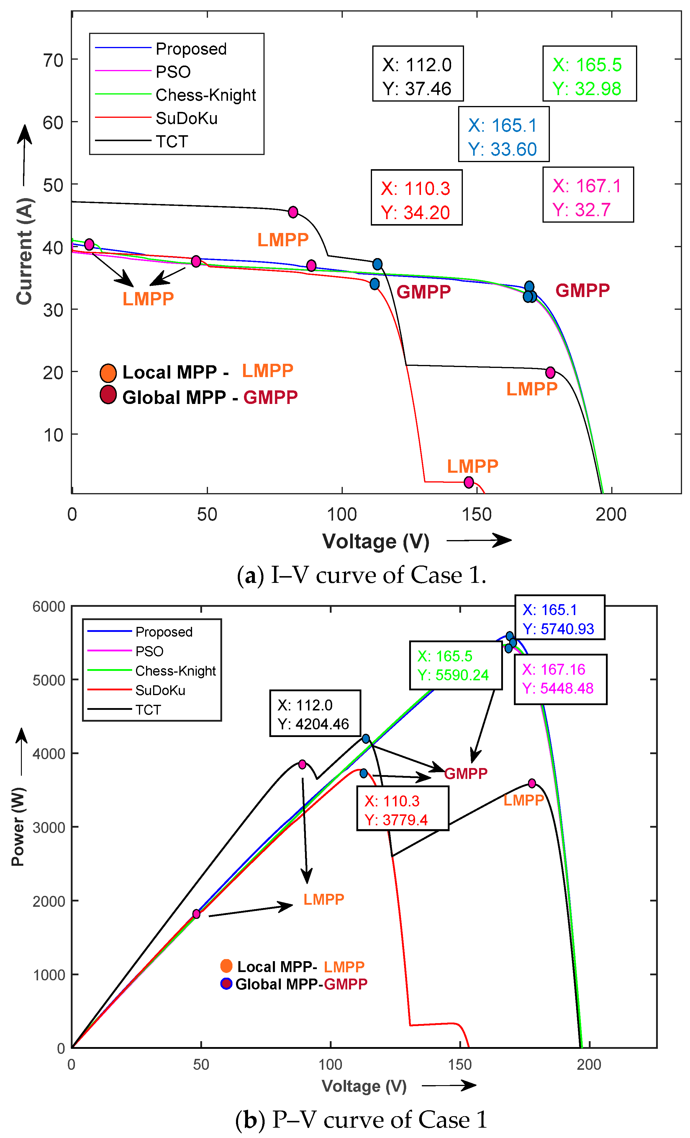
8. Simulation Results and Discussion

This section shows the analyses and simulation results of different shadowing patterns, i.e., (1) short wide, (2) long wide, (3) short narrow, (4) long narrow, and (5) uniform short wide. The latest existing methodologies, such as Chess-Knight Movement, TCT, Sudoku, and PSO, are also simulated and compared for the purpose of validating the results. On the MATLAB/SIMULINK platform, experiments were carried out on a $9\times 9$ PV array built with Kotak $100 \mathrm{W}$ PV modules, making an $8.1 \mathrm{kW}$ total system. Additionally, the theoretical confirmation of the worldwide peak placement was carried out, and the results of the associated simulations relate to the number of bypasses that the $9\times 9$ PV array results in. This research could help to distinguish between various array reconfiguration schemes for big PV arrays. A case study using row current estimate for a first case is used to specifically highlight the number of current changes with TCT, DS, and the suggested technique. This section may be divided by subheadings. It should provide a concise and precise description of the experimental results, their interpretation, and the experimental conclusions that can be drawn.

Case 1: A short, wide pattern

In order to determine the performance of the PV system under shading, most researchers tested their proposed technique on a primary shade case. The standard short wide pattern is shown in Figure 8a. There are four irradiance values for the last four rows of a 9 × 9 TCT PV array, such as 900 $\mathrm{W}/{\mathrm{m}}^2,$600 $\mathrm{W}/{\mathrm{m}}^2$, 400 $\mathrm{W}/{\mathrm{m}}^2$, and 200 $\mathrm{W}/{\mathrm{m}}^2$. The shade dispersion matrices produced for the contemplated short wide pattern using Sudoku, PSO and the suggested Chess-Knight approach are shown in Figure 8b–e. The greatest effect of this shade will be on the TCT interconnection, as the result will be the generation of multiple peaks in the P–V characteristics curve as well as a huge voltage drop.

Table 2. Theoretical calculations for attaining maximum power for Case 1.

TCT Arrangement				Chess-Knight Arrangement
$\mathbf{Row} \mathbf{Currents} {\mathbf{I}}_{\mathbf{m}}$ (A)		$\mathbf{Available} \mathbf{Voltage} {\mathbf{V}}_{\mathbf{m}}$ (V)	$\mathbf{Power} \left({\mathbf{V}}_{\mathbf{m}}{\mathbf{I}}_{\mathbf{m}}\right)$	$\mathbf{Row} \mathbf{Currents} {\mathbf{I}}_{\mathbf{m}}$ (A)		$\mathbf{Available} \mathbf{Voltage} {\mathbf{V}}_{\mathbf{m}}$ (V)	$\mathbf{Power} \left({\mathbf{V}}_{\mathbf{m}}{\mathbf{I}}_{\mathbf{m}}\right)$
Row	Maximum Current			Row	Maximum Current
9	3.6	9	32.4	5	6.1	9	54.9
8	3.6	-	-	6	6.2	8	49.6
7	3.6	-	-	1	6.3	7	44.1
6	6.6	6	39.6	4	-	-	-
5	8.1	5	40.5	8	6.4	5	32
4	8.1	-	-	3	6.5	4	26
3	8.1	-	-	7	6.6	3	19.8
2	8.1	-	-	2	6.7	2	13.4
1	8.1	-	-	9	6.8	1	6.8
Sudoku Arrangement				PSO Arrangement
$\mathbf{Row} \mathbf{Currents} I_m$(A)		$\mathbf{Available} \mathbf{Voltage} V_m$(V)	$\mathbf{Power} (V_m{I}_m$)	$\mathbf{Row} \mathbf{Currents} I_m$ (A)		$\mathbf{Available} \mathbf{Voltage} V_m$(V)	$\mathbf{Power} (V_m{I}_m$)
Row	Maximum Current			Row	Maximum Current
1	6.3	9	56.7	8	6.1	9	54.9
2	-	-	-	2	6.3	8	50.4
6	-	-	-	3	-	-	-
7	-	-	-	5	-	-	-
8	-	-	-	1	6.4	5	32
3	6.6	4	26.4	6	-	-	-
4	-	-	-	4	6.5	3	19.5
5	-	-	-	7	6.8	2	13.6
9	-	-	-	9	-	-	-
Proposed Arrangement
$\mathbf{Row} \mathbf{Currents} I_m$(A)		$\mathbf{Available} \mathbf{Voltage} V_m$(V)	$\mathbf{Power} (V_m{I}_m$)
Row	Maximum Current
5	6.2	9	55.8
2	6.3	8	50.4
6	-	-	-
9	-	-	-
8	6.4	5	32
7	6.5	4	26
4	6.7	3	20.1
1	6.8	2	13.6
3	7	1	7

shows the theoretical representation of the row currents’ difference with voltage bypass and power attainment. TCT attains 40.5 ${\mathrm{V}}_{\mathrm{m}}{\mathrm{I}}_{\mathrm{m}}$ maximum power at 5 ${\mathrm{V}}_{\mathrm{m}}$; however, after relocation, Sudoku attains 56.7 ${\mathrm{V}}_{\mathrm{m}}{\mathrm{I}}_{\mathrm{m}}$ at 9 ${\mathrm{V}}_{\mathrm{m}}$, PSO attains 54.9 ${\mathrm{V}}_{\mathrm{m}}{\mathrm{I}}_{\mathrm{m}}$ at 9 ${\mathrm{V}}_{\mathrm{m}}$, Chess-Knight attains 54.9 ${\mathrm{V}}_{\mathrm{m}}{\mathrm{I}}_{\mathrm{m}}$, also at 9 ${\mathrm{V}}_{\mathrm{m}}$, and the proposed method attains 55.8 ${\mathrm{V}}_{\mathrm{m}}{\mathrm{I}}_{\mathrm{m}}$ of voltage at 9 ${\mathrm{V}}_{\mathrm{m}}$.

Figure 9 displays the simulated characteristics curves of the TCT, PSO, Sudoku, Chess-Knight and the proposed technique. It makes it obvious that the TCT connector accounts for three power peaks, while allowing for three variations in row current, as seen in Table 2. While a linear PV characteristic identical to instances with uniform irradiation has been established, the proposed techniques exhibit narrow row current changes. However, Figure 9a shows more evident changes in I–V characteristics. The proposed row index procedure gives 5740 W, which is more than other existing techniques, such as Chess-Knight, which harnesses 5590.24 W, PSO, with 5448 W, TCT, producing 4204 W, and Sudoku, which gives 3779 W power at output. It has been found that a considerable increase of around 180 W has been recorded compared to the Chess-Knight technique. Additionally, achieving GMPP at maximum voltage simplifies MPP tracking.

Case 2: A long, wide pattern

In this pattern, three neighboring columns and rows are set up to receive various amounts of irradiance to simulate a long, broad shadow pattern. This includes five distinct irradiances, such as 900 $\mathrm{W}/{\mathrm{m}}^2$, 600 $\mathrm{W}/{\mathrm{m}}^2$, 500 $\mathrm{W}/{\mathrm{m}}^2,$ 400 $\mathrm{W}/{\mathrm{m}}^2$ and 200 $\mathrm{W}/{\mathrm{m}}^2,$ on the PV array under consideration. The shade dispersion pattern for interconnected PV arrays is shown in Figure 10a–e, respectively. The greatest effect of this shade will be on the TCT interconnection.

Table 3. Theoretical calculations for attaining maximum power for Case 2.

TCT Arrangement				Chess-Knight Arrangement
$\mathbf{Row} \mathbf{Currents} {\mathbf{I}}_{\mathbf{m}}$ (A)		$\mathbf{Available} \mathbf{Voltage} {\mathbf{V}}_{\mathbf{m}}$ (V)	$\mathbf{Power} \left({\mathbf{V}}_{\mathbf{m}}{\mathbf{I}}_{\mathbf{m}}\right)$	$\mathbf{Row} \mathbf{Currents} {\mathbf{I}}_{\mathbf{m}}$ (A)		$\mathbf{Available} \mathbf{Voltage} {\mathbf{V}}_{\mathbf{m}}$ (V)	$\mathbf{Power} \left({\mathbf{V}}_{\mathbf{m}}{\mathbf{I}}_{\mathbf{m}}\right)$
Row	Maximum Current			Row	Maximum Current
9	3.6	9	32.4	2	5.4	9	48.6
8	3.6	-	-	6	5.5	8	44
7	3.6	-	-	9	-	-	-
6	6.6	6	39.6	1	5.6	6	33.6
5	6.6	-	-	4	-	-	-
4	6.6	-	-	7	-	-	-
3	6.6	-	-	8	-	-	-
2	6.6	-	-	5	5.8	2	11.6
1	6.6	-	-	8	-	-	-
Sudoku Arrangement				PSO Arrangement
$\mathbf{Row} \mathbf{Currents} I_m$(A)		$\mathbf{Available} \mathbf{Voltage} V_m$(V)	$\mathbf{Power} (V_m{I}_m$)	$\mathbf{Row} \mathbf{Currents} I_m$(A)		$\mathbf{Available} \mathbf{Voltage} V_m$(V)	$\mathbf{Power} (V_m{I}_m$)
Row	Maximum Current			Row	Maximum Current
2	5.5	9	49.5	5	5.4	9	48.6
4	-	-	-	8	5.5	8	44
3	5.6	7	39.2	6	-	-	-
5	-	-	-	2	-	-	-
6	-	-	-	4	5.6	5	28
8	-	-	-	9	-	-	-
9	-	-	-	7	5.7	3	17.1
1	5.7	2	11.4	1	-	-	-
7	-	-	-	3	5.9	1	5.9
Proposed Arrangement
$\mathbf{Row} \mathbf{Currents} I_m$(A)		$\mathbf{Available} \mathbf{Voltage} V_m$(V)	$\mathbf{Power} (V_m{I}_m$)
Row	Maximum Current
5	5.4	9	48.6
9	-	-	-
1	5.5	7	38.5
7	-	-	-
2	5.6	5	28
8	-	-	-
3	5.7	3	17.1
4	5.8	2	11.6
6	-	-	-

shows the theoretical representation for the row currents’ difference with voltage bypass and power attainment. TCT attains huge variations in row current, with 39.6 ${\mathrm{V}}_{\mathrm{m}}{\mathrm{I}}_{\mathrm{m}}$ maximum power at 6 $V_m$. However, better optimized variations in row current are noticed with variations, from 5.4${\mathrm{I}}_{\mathrm{m}}$ to 5.8 ${\mathrm{I}}_{\mathrm{m}}$ for Chess-Knight, 5.4${ \mathrm{I}}_{\mathrm{m}}$ to 5.8${\mathrm{I}}_{\mathrm{m}}$ for PSO and 5.5${ \mathrm{I}}_{\mathrm{m}}$ to 5.8${ \mathrm{I}}_{\mathrm{m}}$ for Sudoku, while the proposed technique shows fewer variations in row current, with 5.4${\mathrm{I}}_{\mathrm{m}}$ minimum and 5.7${\mathrm{I}}_{\mathrm{m}}$ maximum value.

Figure 11 shows the simulated characteristics curves of the TCT, PSO, Sudoku, Chess-Knight, and our proposed approach. A linear PV characteristic identical to instances with uniform irradiation was established, and the proposed technique exhibits narrow row current changes. The proposed approach generates 4934 W, compared to 4891 W, 4872 W, 3830 W and 3309 W harnessed by the Chess-Knight, PSO, TCT and Sudoku methods, respectively, for the GMPP power value. It was found that a considerable increase of around 43 W was produced compared to the Chess-Knight technique, though power difference in this pattern is negligible. Any approach that may optimize electricity in this shadow instance has the best potential for being implemented in real time, since wide shade patterns are more likely to occur. Additionally, achieving GMPP at a maximum voltage simplifies MPP tracking.

Case 3: A short, narrow pattern

A small portion of the PV array’s modules are considered while programming a typical short, narrow shadow pattern. Fourteen modules, in this case located at the bottom right corner of PV array, were exposed to this pattern, as shown in Figure 12a–e, respectively. Very few modules are shaded. The power output in all interconnection schemes is expected to be better.

Table 4. Theoretical calculations for attaining maximum power for Case 3.

TCT Arrangement				Chess-Knight Arrangement
$\mathbf{Row} \mathbf{Currents} {\mathbf{I}}_{\mathbf{m}}$ (A)		$\mathbf{Available} \mathbf{Voltage} {\mathbf{V}}_{\mathbf{m}}$ (V)	$\mathbf{Power} \left({\mathbf{V}}_{\mathbf{m}}{\mathbf{I}}_{\mathbf{m}}\right)$	$\mathbf{Row} \mathbf{Currents} {\mathbf{I}}_{\mathbf{m}}$ (A)		$\mathbf{Available} \mathbf{Voltage} {\mathbf{V}}_{\mathbf{m}}$ (V)	$\mathbf{Power} \left({\mathbf{V}}_{\mathbf{m}}{\mathbf{I}}_{\mathbf{m}}\right)$
Row	Maximum Current			Row	Maximum Current
8	6.5	9	58.5	9	7.3	9	65.6
7	6.5	-	-	1	-	-	-
9	6.9	7	48.3	2	-	-	-
6	7.5	6	45	3	7.5	6	45
5	8.1	5	40.5	4	-	-	-
4	-	-	-	5	-	-	-
3	-	-	-	8	7.6	3	22.8
2	-	-	-	6	7.8	2	15.6
1	-	-	-	7	8.1	1	8.1
Sudoku Arrangement				PSO Arrangement
$\mathbf{Row} \mathbf{Currents} I_m$(A)		$\mathbf{Available} \mathbf{Voltage} V_m$(V)	$\mathbf{Power} (V_m{I}_m$)	$\mathbf{Row} \mathbf{Currents} I_m$(A)		$\mathbf{Available} \mathbf{Voltage} V_m$(V)	$\mathbf{Power} (V_m{I}_m$)
Row	Maximum Current			Row	Maximum Current
1	6.8	9	61.2	1	7.3	9	65.6
4	7.3	8	58.4	3	-	-	-
9	-	-	-	5	-	-	-
3	7.5	6	45	6	7.5	6	45
7	-	-	-	8	-	-	-
5	7.8	4	31.2	9	-	-	-
6	-	-	-	4	7.6	3	22.8
2	8.1	2	16.2	2	7.8	2	15.6
8	-	-	-	7	8.1	1	8.1
Proposed Arrangement
$\mathbf{Row} \mathbf{Currents} I_m$(A)		$\mathbf{Available} \mathbf{Voltage} V_m$(V)	$\mathbf{Power} (V_m{I}_m$)
Row	Maximum Current
2	7.3	9	65.7
3	-	-	-
4	7.5	7	52.5
5	-	-	-
6	-	-	-
1	7.6	4	30.4
9	-	-	-
7	7.8	2	15.6
8	-	-	-

shows the theoretical representation for the row currents’ difference, with voltage bypass and power attainment. TCT attains a maximum power of 58.5 $V_m{I}_m$ at a maximum voltage of 6 $V_m$. However, Chess-Knight and PSO are at the same power of 65.6$V_m{I}_m$ at the same voltage level of 9 $V_m$, with huge variations in row current ranges from 7.3 $I_m$ to 8.1 $I_m$, while the proposed technique shows fewer variations in row current, with 7.3 $I_m$ minimum and 7.8 $I_m$ maximum values and maximum power of 65.7 $V_m{I}_m$ at 9$V_m$.

Figure 13 displays the simulated characteristics curves of the TCT, PSO, Sudoku, Chess-Knight and the proposed approach. As the considered shade pattern is not that complex, it ultimately produces less difference in power attainment between all interconnected schemes. The suggested approach produces 6595 W, compared to 6495 W, 6438 W, 5261 W and 4396 W produced by the Chess-Knight, PSO, TCT and Sudoku methods, respectively, for the GMPP power value. Be aware that, as compared to that approach, a considerable increase of around 100 W has been produced compared to the Chess-Knight technique, though power difference in this pattern is negligible.

Case 4: A long, narrow pattern

The last five columns of the TCT linked PV array are expected to be shaded to achieve a long narrow shadow scenario. The representation of interconnected PV arrays subjected to this pattern for shade dispersion are shown in Figure 14a–e, respectively. For critical performance evaluation, the pattern selected is unusual which means the shade is not uniform across five columns.

Table 5. Theoretical calculations for attaining maximum power for Case 4.

TCT Arrangement				Chess-Knight Arrangement
$\mathbf{Row} \mathbf{Currents} {\mathbf{I}}_{\mathbf{m}}$ (A)		$\mathbf{Available} \mathbf{Voltage} {\mathbf{V}}_{\mathbf{m}}$ (V)	$\mathbf{Power} \left({\mathbf{V}}_{\mathbf{m}}{\mathbf{I}}_{\mathbf{m}}\right)$	$\mathbf{Row} \mathbf{Currents} {\mathbf{I}}_{\mathbf{m}}$ (A)		$\mathbf{Available} \mathbf{Voltage} {\mathbf{V}}_{\mathbf{m}}$ (V)	$\mathbf{Power} \left({\mathbf{V}}_{\mathbf{m}}{\mathbf{I}}_{\mathbf{m}}\right)$
Row	Maximum Current			Row	Maximum Current
9	5.1	9	45.9	9	6.1	9	54.9
8	5.1	-	-	1	6.8	8	54.4
7	6.1	7	42.7	2	-	-	-
6	6.1	-	-	3	-	-	-
5	7.5	5	37.5	7	-	-	-
4	7.5	-	-	8	-	-	-
3	8.1	3	24.3	4	7.1	3	21.3
2	8.1	-	-	5	-	-	-
1	8.1	-	-	6	7.5	1	7.5
Sudoku Arrangement				PSO Arrangement
$\mathbf{Row} \mathbf{Currents} I_m$(A)		Available Voltage$V_m$(V)	Power ($V_m{I}_m$)	Row Currents$I_m$(A)		Available Voltage$V_m$(V)	Power ($V_m{I}_m$)
Row	Maximum Current			Row	Maximum Current
4	5.9	9	53.1	8	6	9	54
7	6.4	8	51.2	2	6.7	8	53.6
1	6.5	7	45.5	1	-	-	-
9	6.8	6	40.8	5	-	-	-
3	7	5	35	4	-	-	-
6	7.1	4	28.4	7	-	-	-
2	7.2	3	21.6	3	7	3	21
8	7.3	2	14.6	9	-	-	-
5	7.5	1	7.5	6	7.3	1	7.3
Proposed Arrangement
$\mathbf{Row} \mathbf{Currents} V_m$(A)		Available Voltage$V_m$(V)	Power ($V_m{I}_m$)
Row	Maximum Current
8	6.2	9	55.8
1	6.8	8	54.4
2	-	-	-
3	-	-	-
4	-	-	-
9	-	-	-
5	7	3	21
6	-	-	-
7	7.5	1	7.5

shows the theoretical calculations for maximum power. TCT attains the maximum power of 45.9 $V_m{I}_m$ at a maximum voltage of 9$V_m$. However, Chess-Knight attains a maximum power of 54.9 $V_m{I}_m$ at 9$V_m$ and PSO attains maximum power of 54 $V_m{I}_m$ at 9$V_m$, with huge variations in row current, while the proposed technique shows fewer variations in row current, with 6.2 $I_m$ minimum and 7.5$I_m$ maximum values, with a maximum power of 55.8 $V_m{I}_m$ at 9$V_m$.

Figure 15 displays the simulated characteristic curves of the TCT, PSO, Sudoku, Chess-Knight, and proposed technique. As the considered shade pattern is not that complex, it ultimately produces less difference in the power attainment between all interconnected schemes. The suggested approach produces 5945 W, compared to 5915 W, 5845 W, 5016 W and 4001 W produced by Chess-Knight, PSO, TCT and Sudoku methods, respectively, for the GMPP power value. Be aware that, as compared to that approach, a considerable increase of around 30 W was produced compared to the Chess-Knight technique, though the power difference in this pattern is negligible. Despite multiple peak issues with TCT and Sudoku interconnections, the proposed technique dominates by enhancing output power.

Case 5: A uniform, short, wide pattern

Real-time PV arrays suffer significant hindrances when there are short, broad shadow instances. The shade dispersion matrices produced for the contemplated short, wide pattern using TCT, Sudoku, PSO and the suggested Chess-Knight approach are shown in Figure 16a–e. The greatest effect of this shade will be on the TCT interconnection, as the result will be the generation of multiple peaks in the P–V characteristics curve as well as a huge voltage drop.

Table 6. Theoretical calculations for attaining maximum power for Case 5.

TCT Arrangement				Chess-Knight Arrangement
$\mathbf{Row} \mathbf{Currents} {\mathbf{I}}_{\mathbf{m}}$ (A)		$\mathbf{Available} \mathbf{Voltage} {\mathbf{V}}_{\mathbf{m}}$ (V)	$\mathbf{Power} \left({\mathbf{V}}_{\mathbf{m}}{\mathbf{I}}_{\mathbf{m}}\right)$	$\mathbf{Row} \mathbf{Currents} {\mathbf{I}}_{\mathbf{m}}$ (A)		$\mathbf{Available} \mathbf{Voltage} {\mathbf{V}}_{\mathbf{m}}$ (V)	$\mathbf{Power} \left({\mathbf{V}}_{\mathbf{m}}{\mathbf{I}}_{\mathbf{m}}\right)$
Row	Maximum Current			Row	Maximum Current
9	3.6	9	32.4	6	6.2	9	55.8
8	3.6	-	-	5	6.4	8	51.2
7	3.6	-	-	8	-	-	-
6	8.1	6	48.6	1	6.6	6	39.6
5	8.1	-	-	4	-	-	-
4	8.1	-	-	7	-	-	-
3	8.1	-	-	3	6.8	3	20.4
2	8.1	-	-	9	-	-	-
1	8.1	-	-	2	7	1	7
Sudoku Arrangement				PSO Arrangement
$\mathbf{Row} \mathbf{Currents} I_m$(A)		$\mathbf{Available} \mathbf{Voltage} V_m$(V)	$\mathbf{Power} (V_m{I}_m$)	$\mathbf{Row} \mathbf{Currents} I_m$(A)		$\mathbf{Available} \mathbf{Voltage} V_m$(V)	$\mathbf{Power} (V_m{I}_m$)
Row	Maximum Current			Row	Maximum Current
1	6.2	9	55.8	4	6.2	9	55.8
4	-	-	-	5	6.3	8	50.4
8	6.4	7	44.8	8	-	-	-
5	6.6	6	39.6	7	6.5	6	39
9	-	-	-	2	6.8	5	34
2	6.8	4	27.2	3	-	-	-
3	-	-	-	5	-	-	-
7	-	-	-	9	-	-	-
6	7	1	7	1	7	1	7
Proposed Arrangement
$\mathbf{Row} \mathbf{Currents} I_m$(A)		Available Voltage$V_m$(V)	Power ($V_m{I}_m$)
Row	Maximum Current
7	6.2	9	55.8
6	6.4	8	51.2
9	-	-	-
2	6.6	6	39.6
5	-	-	-
8	-	-	-
1	6.8	3	20.4
4	-	-	-
3	7	1	7

shows the theoretical representation for the row currents’ difference with voltage bypass and power attainment. It can be seen that TCT attains a 32.4 $V_m{I}_m$ maximum power at 9$V_m$; however, after relocation, Sudoku attains 55.8 $V_m{I}_m$ at 9$V_m$, PSO attains 55.8 $V_m{I}_m$ at 9 $V_m$, Chess-Knight attains 55.8 $V_m{I}_m$, also at 9$V_m$, and the proposed method attains 55.8 $V_m{I}_m$ of voltage at 9 $V_m$.

Figure 17a,b display the simulated characteristic curves of the TCT, PSO, Sudoku, Chess-Knight, and the proposed approach. A very linear PV characteristic identical to instances with uniform irradiation has been established, and the proposed and other techniques exhibit narrow row current changes. However, Figure 17a shows more evident changes in I–V characteristics. The suggested approach produces 5796 W, compared to 5672 W, 5643 W, 4718 W and 3298 W produced by the Chess-Knight, PSO, TCT and Sudoku methods, respectively, for the GMPP power value. Be aware that, as compared to that approach, a considerable increase of around 124 W was produced compared to the Chess-Knight technique. Any approach that may optimize electricity in this shadow instance has the best potential of being implemented in real time, since wide shade patterns are more likely to occur. Additionally, achieving GMPP at a maximum voltage simplifies MPP tracking.

The following crucial conclusions are drawn from the simulation and results analysis carried out using the five shade cases:

• The row index based reconfiguration technique is easy to build and has a high degree of reliability for dispersing the shadow in any of the scenarios;
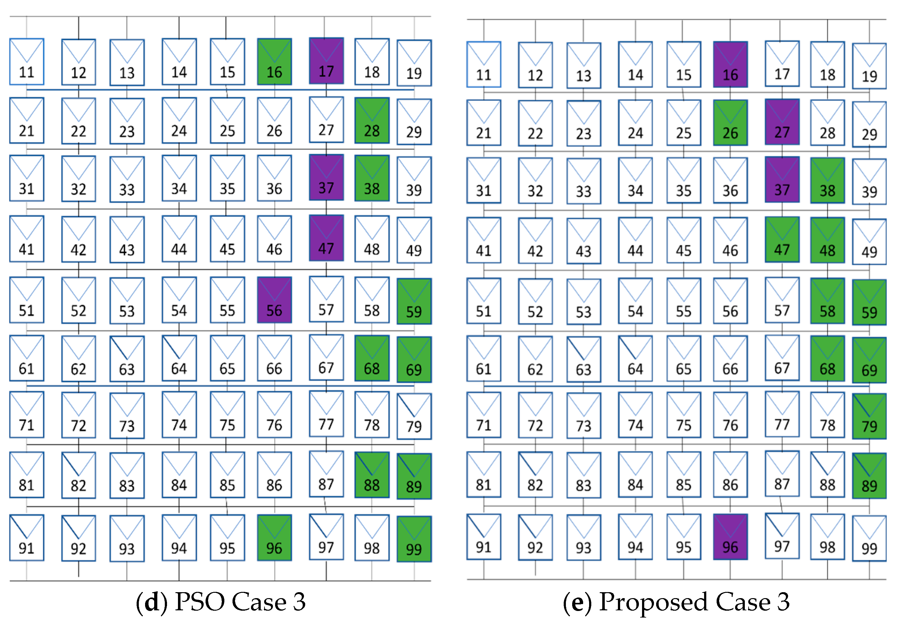
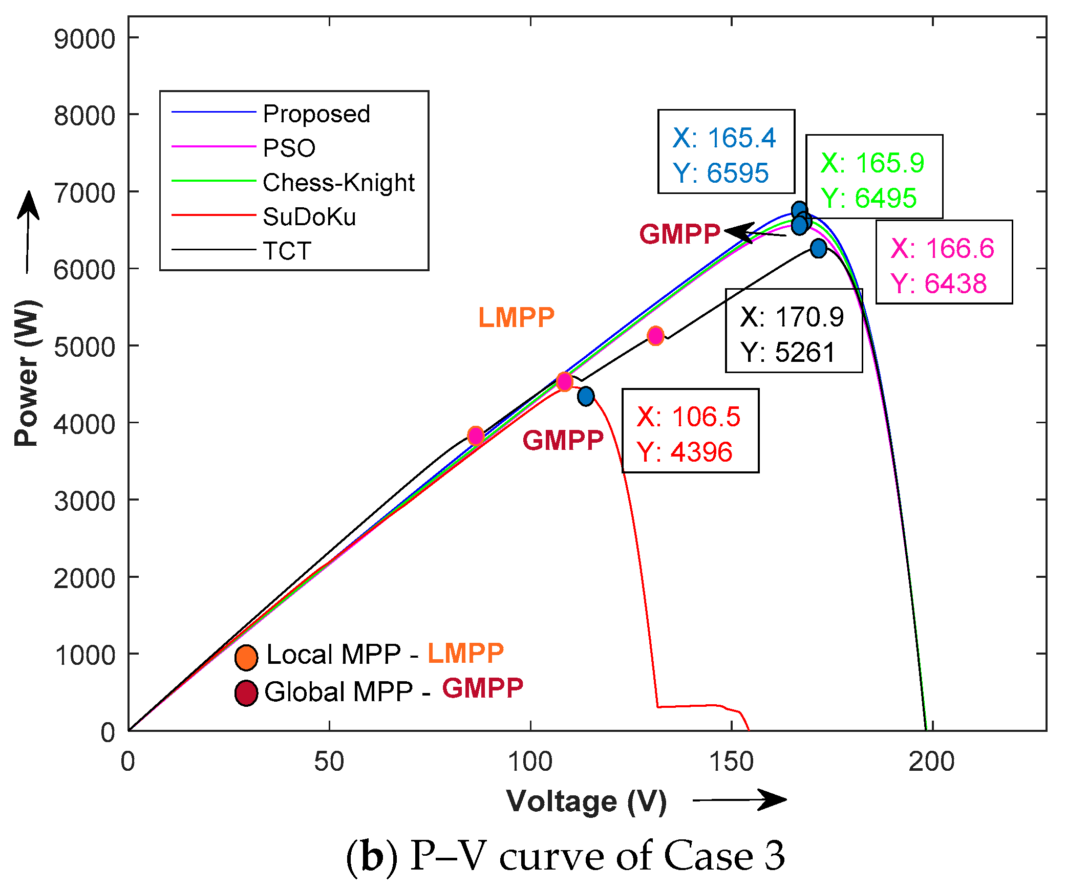
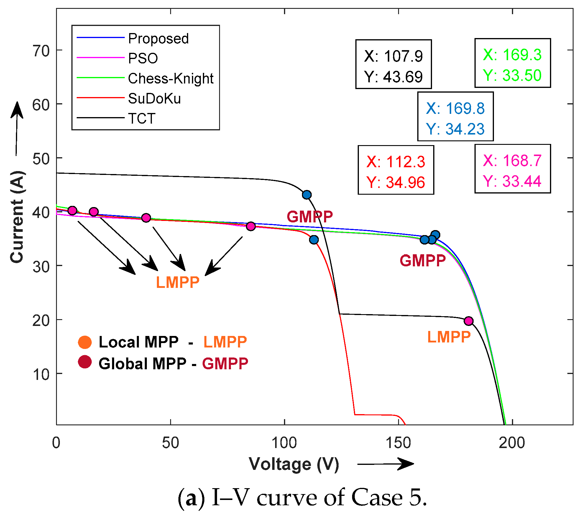
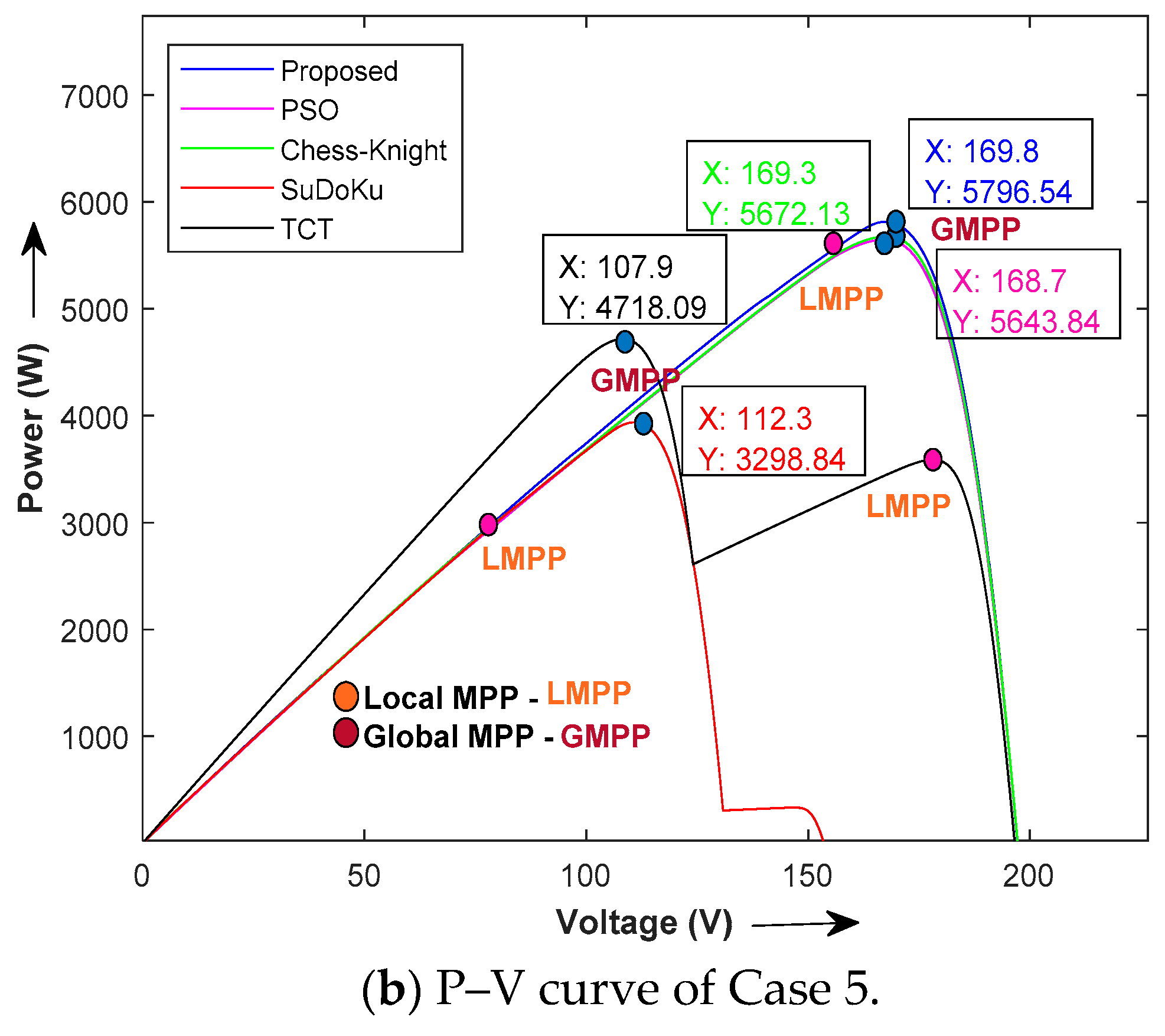
• This approach is the most appropriate method for the shade dispersion process when compared to recently published techniques such as PSO, the Chess-Knight method and typical reconfiguration techniques such as Sudoku and TCT. PSO and Chess-Knight have better results than others, and therefore these two latest techniques are shortlisted and implemented against shadowing scenarios;
• Regardless of the location of the global power point, the physical relocation’s circuit complexity is a key consideration when choosing a technique.

9. Conclusions

This research proposes a novel row index based reconfiguration scheme. Array reconfiguration techniques based on physical relocation are highlighted as some of the finest solutions to optimize power under shadow occurrences. The row index based reconfiguration strategy has been especially created and tested for identifying the potential of physical relocation by employing basic mathematics. Our proposed technique is evaluated against five different shadow patterns in an 8.1 $\mathrm{kW}$ system ($9\times 9$) PV array to confirm its ability to optimize row current, disperse shade and improve power. Overall, with sufficient validation, the row index approach has been advanced and thoroughly tested to be an absolute and reliable choice for big PV array reconfiguration processes. In terms of future scope, array reconfiguration strategies for outdated PV arrays and panel degradation are a new way of looking at solutions. It was found that approximately 68$\%$ of power loss is mitigated when compared to TCT. It was also observed that the proposed technique yields more power than recently published Sudoku, Chess-Knight and PSO based reconfigured techniques. Furthermore, array reconfiguration strategies linked to a grid-connected system may provide a broad scope for PV system study.

References

1. Ullah, K.I.; Azhar, U.-H.; Yousef, M.; Marium, J.; Muhammad, A.; Ullah, A.M.; Khalid, M. Comparative Analysis of Photovoltaic Faults and Performance Evaluation of its Detection Techniques. IEEE Access 2020, 8, 26676–26700. [Google Scholar] [CrossRef]
2. Kaleem, A.; Khalil, I.U.; Aslam, S.; Ullah, N.; Al Otaibi, S.; Algethami, M. Feedback PID Controller-Based Closed-Loop Fast Charging of Lithium-Ion Batteries Using Constant-Temperature–Constant-Voltage Method. Electronics 2021, 10, 2872. [Google Scholar] [CrossRef]
3. Deshkar, S.N.; Dhale, S.B.; Mukherjee, J.S.; Babu, T.S.; Rajasekar, N. Solar PV array reconfiguration under partial SHading conditions for maximum power extraction using genetic algorithm. Renew. Sustain. Energy Rev. 2015, 43, 102–110. [Google Scholar] [CrossRef]
4. Osmani, K.; Haddad, A.; Jaber, H.; Lemenand, T.; Castanier, B.; Ramadan, M.R. Mitigating the effects of partial shading on PV system’s performance through PV array reconfiguration: A review. Therm. Sci. Eng. Prog. 2022, 31, 101280. [Google Scholar] [CrossRef]
5. An Efficient SD-PAR Technique for Maximum Power Generation from Modules of Partially Shaded PV Arrays—ScienceDirect. Available online: https://www.sciencedirect.com/science/article/pii/S0360544219304827 (accessed on 26 June 2022).
6. Rezazadeh, S.; Moradzadeh, A.; Pourhossein, K.; Akrami, M.; Mohammadi-ivatloo, B.; Anvari-Moghaddam, A. Photovoltaic array reconfiguration under partial shading conditions for maximum power extraction: A state-of-the-art review and new solution method. Energy Convers. Manag. 2022, 258, 115468. [Google Scholar] [CrossRef]
7. Design and Testing of Two Phase Array Reconfiguration Procedure for Maximizing Power in Solar PV Systems under Partial Shade Conditions (PSC)—ScienceDirect. Available online: https://www.sciencedirect.com/science/article/pii/S0196890418311208 (accessed on 26 June 2020).
8. Al-Dousari, A.M.; Al-Nassar, W.; Al-Hemoud, A.; Alsaleh, A.; Ramadan, A.; Al-Dousari, N.; Ahmed, M. Solar and wind energy: Challenges and solutions in desert regions. Energy 2019, 176, 184–194. [Google Scholar] [CrossRef]
9. Optimization of Photovoltaic Energy Production through an Efficient Switching Matrix. Available online: https://www.researchgate.net/publication/261296842_Optimization_of_Photovoltaic_Energy_Production_through_an_Efficient_Switching_Matrix (accessed on 26 June 2022).
10. An Adaptive Utility Interactive Photovoltaic System Based on a Flexible Switch Matrix to Optimize Performance in Real-Time—ScienceDirect. Available online: https://www.sciencedirect.com/science/article/pii/S0038092X12000175 (accessed on 26 June 2022).
11. The Optimized-String Dynamic Photovoltaic Array. Available online: https://www.researchgate.net/publication/260496754_The_Optimized-String_Dynamic_Photovoltaic_Array (accessed on 26 June 2022).
12. Babu, T.S.; Ram, J.P.; Dragičević, T.; Miyatake, M.; Blaabjerg, F.; Rajasekar, N. Particle Swarm Optimization Based Solar PV Array Reconfiguration of the Maximum Power Extraction Under Partial Shading Conditions. IEEE Trans. Sustain. Energy 2018, 9, 74–85. [Google Scholar] [CrossRef]
13. Extended Analysis on Line-Line and Line-Ground Faults in PV Arrays and a Compatibility Study on Latest NEC Protection Standards—ScienceDirect. Available online: https://www.sciencedirect.com/science/article/pii/S0196890419307137 (accessed on 26 June 2022).
14. Maximizing the Power Generation of a Partially Shaded PV Array|IEEE Journals & Magazine|IEEE Xplore. Available online: https://ieeexplore.ieee.org/document/7320967 (accessed on 26 June 2022).
15. Performance Enhancement of Partially Shaded PV Array Using Novel Shade Dispersion Effect on Magic-Square Puzzle Configuration—ScienceDirect. Available online: https://www.sciencedirect.com/science/article/pii/S0038092X17300208 (accessed on 26 June 2022).
16. Comprehensive Investigation of PV Arrays with Puzzle Shade Dispersion for Improved Performance—ScienceDirect. Available online: https://www.sciencedirect.com/science/article/pii/S0038092X16000803 (accessed on 26 June 2022).
17. Power Enhancement of PV System via Physical Array Reconfiguration Based Lo Shu Technique—ScienceDirect. Available online: https://www.sciencedirect.com/science/article/pii/S0196890420304234 (accessed on 26 June 2022).
18. Meerimatha, G.; Rao, B.L. Novel reconfiguration approach to reduce line losses of the photovoltaic array under various shading conditions. Energy 2020, 196, 117120. [Google Scholar] [CrossRef]
19. Krishna, G.S.; Moger, T. Enhancement of maximum power output through reconfiguration techniques under non-uniform irradiance conditions. Energy 2019, 187, 115917. [Google Scholar] [CrossRef]
20. Dhanalakshmi, B.; Rajasekar, N. Dominance square based array reconfiguration scheme for power loss reduction in solar PhotoVoltaic (PV) systems. Energy Convers. Manag. 2018, 156, 84–102. [Google Scholar] [CrossRef]
21. A novel Competence Square Based PV Array Reconfiguration Technique for Solar PV Maximum Power Extraction|Request PDF. Available online: https://www.researchgate.net/publication/327514830_A_novel_Competence_Square_based_PV_array_reconfiguration_technique_for_solar_PV_maximum_power_extraction (accessed on 26 June 2022).
22. A Novel Zig-Zag Scheme for Power Enhancement of Partially Shaded Solar Arrays—ScienceDirect. Available online: https://www.sciencedirect.com/science/article/pii/S0038092X16301529 (accessed on 26 June 2022).
23. A Simple, Sensorless and Fixed Reconfiguration Scheme for Maximum Power Enhancement in PV Systems—ScienceDirect. Available online: https://www.sciencedirect.com/science/article/pii/S0196890418307416 (accessed on 26 June 2022).
24. A New Shade Dispersion Technique Compatible for Symmetrical and Unsymmetrical Photovoltaic (PV) Arrays—ScienceDirect. Available online: https://www.sciencedirect.com/science/article/pii/S0360544221004904 (accessed on 26 June 2022).
25. Sai Krishna, G.; Moger, T. Improved SuDoKu reconfiguration technique for total cross-tied PV array to enhance maximum power under partial shading condition. Renew Sustain. Energy Rev. 2019, 109, 333–348. [Google Scholar] [CrossRef]
26. Posture, S.R.; Pattabiraman, D.; Ganesan, S.I.; Chilakapati, N. Positioning of PV panels for reduction in line losses and mismatch losses in PV array. Renew. Energy 2015, 78, 264–275. [Google Scholar] [CrossRef]
27. Tabanjat, A.; Becherif, M.; Hissel, D. Reconfiguration solution for shaded PV panels using switching control. Renew. Energy 2015, 82, 4–13. [Google Scholar] [CrossRef]
28. Karakose, M.; Baygin, M.; Parlak, K.S.; Baygin, N.; Akin, E. A novel reconfiguration method using image processing based moving shadow detection, optimization, and analysis for PV Arrays. J. Inf. Sci. Eng. 2018, 34, 1307–1328. [Google Scholar] [CrossRef]
29. Reconfiguration Strategies to Extract Maximum Power from Photovoltaic Array under Partially Shaded Conditions—ScienceDirect. Available online: https://www.sciencedirect.com/science/article/pii/S136403211731033X (accessed on 26 June 2022).
30. Computation of Power Extraction from Photovoltaic Arrays under Various Fault Conditions|IEEE Journals & Magazine|IEEE Xplore. Available online: https://ieeexplore.ieee.org/document/9040695 (accessed on 26 June 2022).
31. A Novel Chaotic Flower Pollination Algorithm for Global Maximum Power Point Tracking for Photovoltaic System under Partial Shading Conditions|IEEE Journals & Magazine|IEEE Xplore. Available online: https://ieeexplore.ieee.org/document/8813051 (accessed on 26 June 2022).
32. Maximum Power Extraction in Solar Renewable Power System—A Bypass Diode Scanning Approach—ScienceDirect. Available online: https://www.sciencedirect.com/science/article/pii/S0045790617308066 (accessed on 26 June 2022).
33. Ndiaye, A.; Kébé, C.; Charki, A.; Sambou, V.; Ndiaye, P. Photovoltaic Platform for Investigating PV Module Degradation. Energy Procedia 2015, 74, 1370–1380. [Google Scholar] [CrossRef] [Green Version]
34. Variations of the Bacterial Foraging Algorithm for the Extraction of PV Module Parameters from Nameplate Data—ScienceDirect. Available online: https://www.sciencedirect.com/science/article/pii/S019689041630019X (accessed on 26 June 2022).
35. Discrete I–V Model for Partially Shaded PV-Arrays—ScienceDirect. Available online: https://www.sciencedirect.com/science/article/pii/S0038092X14000668 (accessed on 26 June 2022).
36. Application of Bio-Inspired Algorithms in Maximum Power Point Tracking for PV Systems under Partial Shading Conditions—A Review—ScienceDirect. Available online: https://www.sciencedirect.com/science/article/pii/S1364032117311760 (accessed on 26 June 2022).
37. A Review on Factors Influencing the Mismatch Losses in Solar Photovoltaic System. Available online: https://www.hindawi.com/journals/ijp/2022/2986004/ (accessed on 26 June 2022).
38. Ram, J.P.; Rajasekar, N. A Novel Flower Pollination Based Global Maximum Power Point Method for Solar Maximum Power Point Tracking. IEEE Trans. Power Electron. 2017, 32, 8486–8499. [Google Scholar] [CrossRef]
Figure 1. Different interconnections schemes of PV array: (a) SP arrangement; (b) TCT arrangement; (c) BL arrangement; (d) Honeycomb arrangement.
Symmetry 15 00768 g001
Figure 2. Overview of PV structure and equivalent circuit of PV cells, as in [4].
Symmetry 15 00768 g002
Figure 3. Characteristics curves with multiple peaks and an overview of mitigation methods.
Symmetry 15 00768 g003aSymmetry 15 00768 g003bSymmetry 15 00768 g003c
Figure 4. Classification of mismatch faults in PV arrays.
Symmetry 15 00768 g004
Figure 5. PV array reconfiguration via a physical relocation procedure and the partial shade effect on TCT, and the proposed technique with the P–V characteristics curve.
Symmetry 15 00768 g005
Figure 6. Reconfiguration of 9 × 9 PV array using the row index method.
Symmetry 15 00768 g006aSymmetry 15 00768 g006bSymmetry 15 00768 g006c
Figure 7. Flow chart of proposed row index based reconfiguration procedure.
Symmetry 15 00768 g007
Figure 8. Shade dispersion in TCT, Chess-Knight, Sudoku, PSO and the proposed scheme for Case 1.
Symmetry 15 00768 g008
Figure 9. Simulated I–V and P–V curves for Case 1.
Symmetry 15 00768 g009
Figure 10. Shade dispersion in TCT, Chess-Knight, Sudoku, PSO and the proposed scheme for Case 2.
Symmetry 15 00768 g010aSymmetry 15 00768 g010b
Figure 11. Simulated I–V and P–V characteristics for Case 2.
Symmetry 15 00768 g011aSymmetry 15 00768 g011b
Figure 12. Shade dispersion in TCT, Chess-Knight, Sudoku, PSO and the proposed scheme for Case 3.
Symmetry 15 00768 g012aSymmetry 15 00768 g012b
Figure 13. Simulated I–V and P–V characteristics for Case 3.
Symmetry 15 00768 g013aSymmetry 15 00768 g013b
Figure 14. Shade dispersion in TCT, Chess-Knight, Sudoku, PSO and the proposed scheme for test Case 4.
Symmetry 15 00768 g014aSymmetry 15 00768 g014b
Figure 15. Simulated I–V and P–V characteristics for Case 4.
Symmetry 15 00768 g015aSymmetry 15 00768 g015b
Figure 16. Shade dispersion in TCT, Chess-Knight, Sudoku, PSO and the proposed scheme for test Case 5.
Symmetry 15 00768 g016aSymmetry 15 00768 g016b
Figure 17. Simulated I–V and P–V characteristics for Case 5.
Symmetry 15 00768 g017aSymmetry 15 00768 g017b