A Malware Detection Approach Based on Deep Learning and Memory Forensics

Abstract

As cyber attacks grow more complex and sophisticated, new types of malware become more dangerous and challenging to detect. In particular, fileless malware injects malicious code into the physical memory directly without leaving attack traces on disk files. This type of attack is well concealed, and it is difficult to find the malicious code in the static files. For malicious processes in memory, signature-based detection methods are becoming increasingly ineffective. Facing these challenges, this paper proposes a malware detection approach based on convolutional neural network and memory forensics. As the malware has many symmetric features, the saved training model can detect malicious code with symmetric features. The method includes collecting executable static malicious and benign samples, running the collected samples in a sandbox, and building a dataset of portable executables in memory through memory forensics. When a process is running, not all the program content is loaded into memory, so binary fragments are utilized for malware analysis instead of the entire portable executable (PE) files. PE file fragments are selected with different lengths and locations. We conducted several experiments on the produced dataset to test our model. The PE file with 4096 bytes of header fragment has the highest accuracy. We achieved a prediction accuracy of up to 97.48%. Moreover, an example of fileless attack is illustrated at the end of the paper. The results show that the proposed method can detect malicious codes effectively, especially the fileless attack. Its accuracy is better than that of common machine learning methods.

1. Introduction

With the development of internet technology, malware attacks became more prevalent and sophisticated. Currently, malware is one of the dominant attack vectors used by cybercriminals to perform malicious activities [1]. Everyday, the AV-TEST Institute registers over 450,000 new malicious programs (malware) and potentially unwanted applications (PUA) [2]. Antivirus products implement static and heuristic analysis technologies to detect malware. Unfortunately, these approaches became less effective to detect sophisticated malware that exploits obfuscation and encryption techniques [3]. In particular, fileless malware attacks are wildly used and cause severe losses. Fileless malware is a type of malicious software that does not rely on files and leaves no footprint on the computer disk. It is difficult to detect unknown malicious programs without knowing their signatures.

To combat such threats, much research is carried out in various fields, including deep learning, memory forensics, number theory, and so on [4,5,6]. Memory forensics offers unique insights into the internal state of kernel system and running programs [7]. Memory has a high potential to contain malicious code from an infection, in whole or in part, even if it is never written to disk, because it must be loaded in memory to execute [8]. The analysis target of memory forensics is a memory dump from where the attack traces can be extracted. By contrast, these traces are not available by the traditional disk analysis method. During memory analysis, malwares are executed in a sandbox to prevent the malwares from causing damage to the entire computer system, which is accomplished by establishing virtual machines. Memory data must be collected in a timely manner when malware is running on the virtual machine (VM). In this paper, the memory data are dumped to the disk using the memory dump algorithm for further analysis. In addition to dumping the memory data, malicious portable executable (PE) files must be extracted from thousands of memory data as sample data. Bozkir et al. [9] presented an approach to recognize malware by capturing the memory dump of suspicious processes, which can be represented as an RGB image. However, collecting malicious memory data in this manner is inadequate. The extracted process potentially did not load malicious code into memory. Some malicious processes are injected into new processes to perform malicious actions. In this case, extracting a single malicious process cannot fully reflect the malicious behavior of the process. Only extracting a malicious running single process cannot fully reflect the value of memory analysis. The dataset in this paper takes multiple dumps of memory images and extracts all processes and DLL data. By close analysis of this information, benign and malicious data can be classified through a detection platform.

This paper proposes a malicious code detection method. A neural network model is built to detect sample fragments. The sample fragment’s time cost is reduced compared to detecting the whole sample. To reduce the problem of crucial data loss caused by sample fragment detection, we select fragments by detecting different positions and lengths to determine the appropriate place and size of the detected segments.

The main contributions of this paper are summarized as follows:

• This paper builds a portable executable (PE) file dataset in memory, which extracts more malicious memory samples in the process. This paper first collects static PE files from the well-known malicious sample libraries VirusShare and MalShare, which are widely used by researchers and have high persuasiveness. Then, this paper downloads the common software from the official Microsoft platform. Finally, it executes the static samples in running virtual machines and extracts the dynamic samples to create our dataset;
• We build a model based on the neural network (CNN), and use the model to train memory segments to achieve accurate detection of malicious code;
• We give an example of fileless malware attack in the paper. Since the dynamic file dataset is constructed, it has good detection performance for “no file” attacks and malicious samples that can only be detected in dynamic files.

2. Related Work

2.1. Memory Forensics

The computer forensics approaches are divided into the dynamic and static analysis. Static analysis is built on the premise of not running the program. It includes the extraction process of components, instructions, control flow, and function calling of sequence static code features, such as anomaly detection [10]. Jiang et al. [11] designed a set of fine-grained binary integrity verification schemes to check the integrity of binary files in virtual machines. The static analysis method had high sample coverage. Still, a multi-angle analysis was required to detect malicious code using technologies such as deformation, polymorphism, code obfuscation, and encryption [12]. Regarding dynamic analysis, most of the information in the memory was incomplete owing to the paging and replacement mechanism of the memory. The program did not transfer all the information into the memory during execution. Only part of the information was moved into the memory first. Therefore, the complete executable data cannot be obtained.

Furthermore, once a malicious program detects that the virus/Trojan detection tool was running or using software to obtain the memory, it immediately interrupts the attack behavior, self-destructs, and erases the attack traces. These self-destruction behaviors put forward higher requirements for memory data sampling and detection. Otsuki et al. [13] proposed a method of extracting stack traces from the memory images in a 64-bit Windows system. They demonstrated the effectiveness of Stealth Loader by analyzing a set of Windows executables and malware protected with Stealth Loader using major dynamic and static analysis tools. Uroz et al. [14] investigated the limitations that memory forensics impose to the digital signature verification process of Windows PE-signed files obtained from a memory dump. These limitations are data incompleteness, data changes caused by relocation, catalog-signed files, and executable file and process inconsistencies. Cheng et al. [15] proposed a clustering algorithm that realized the automatic memory data correlation analysis method through analyzing the critical data structure of the operating system. The main ideas are guaranteeing data accuracy in multi-view extraction and analyzing memory behavior in a para-synchronous style. Palutke [16] exploited a memory sharing mechanism to detect hidden processes from memory data. They present three novel methods that prevent malicious user space memory from appearing in analysis tools and additionally making the memory inaccessible from a security analysts perspective. Wang et al. [17] adopted the Windows physical memory analysis method based on the KPCR (Kernel’s Processor Control Region) structure, which solved the problems of the version judgment and the address translation of the operating system. It became increasingly challenging to conduct memory forensics using the above methods for the exponentially increasing malicious codes. It is difficult to detect whether there are malicious behaviors in a large number of in-memory PE files through professional manual analysis, which makes it a very challenging research direction.

2.2. Malware Detection

Malicious code detection approaches are popular among network security researchers. To judge whether the exe file is malicious software, the entire static exe file is dealt with using a machine learning algorithm [18]. The disadvantage of this method is that if the amount of data in the dataset was enormous, an oversized load was generated during the data training process. In the way proposed by Bozkir et al. [9], the binary files of the malicious samples are converted into images, and the transformed images are classified by the classifiers support vector machines (SVM), extreme gradient boosting (XGBoost), and random forest. Marín et al. [19] extracted printable characters from the PE files for detection through machine learning. Li et al. [20] proposed a CNN-based malware detection approach. The vgg-16 model was used as their train model in which convolutional filters were of the size 3 × 3. Zhang et al. [21] proposed a classification method for malware. The process extracted the semantic structure features of the code based on a data flow analysis and used graph convolutional networks to detect the semantic structural features. The detection accuracy of this method was 95.8%. Wadkar et al. [22] proposed an evolutionary detection method for malware based on the SVM model. The method proposed by Han et al. [23] analyzes malware based on its structure and behavior.

Subsequently, several classifiers, namely, random forest, decision tree, CNN, and XGBoost, were used to classify the input data. Huang et al. [24] developed a malware detection method using deep learning and visualization based on Windows API. It generates static visualizations using static features retrieved from the sample files. Lu XD et al. [25] proposed an malicious code deep forest (MCDF) detection approach. In the process, binary files were converted to grayscale images, which were used for training and testing of the MCDF model.

As discussed above, most research methods used memory data structures and connections between processes for memory forensics and malicious code detection. It is often tough to find specific malware using these methods. Some previously proposed methods [5,12,26] analyzed specific memory files; another previously reported way [14] examines the registry in the memory. A previous study [9] proposed a method that converts memory files into images for analysis through machine learning. In the existing research methods, the dataset is basically static data or only a single process file. The malicious behavior injected into other processes cannot be detected. We extract all processes and DLL files from memory to detect malicious code, especially fileless attacks. Additionally, we maximize the creation of memory PE datasets by extracting malicious files from memory. Finally, we build a deep learning model that fits our data. Typical anti-malware techniques are mostly based on signatures to determine whether software contains malicious code. Uroz et al. [14] developed the volatility plugin sigcheck, which recovers executable files from a memory dump and computes its digital signature (if feasible). They tested it on Windows 7 x86 and x64 memory dumps. Their method requires capturing the full PE file and its detection rate gets lower and lower as the code runs. However, by detecting file fragments, our method is more efficient. By performing several sets of experiments on the produced dataset, we conclude that the 4096-byte data fragment at the head of the PE file in the memory is used for detection and the accuracy rate is 97.48%.

3. Memory PE File Extraction Technology

3.1. Memory Analysis

Memory forensics rely on the memory image’s binary file. It is challenging to locate and analyze the valuable information from the dumped memory image. Although a process is very similar to a program on the surface, the concept of a process is essentially different. A program is a static sequence of instructions. The process is a dynamic operation that contains the sequence of execution and various resources to execute the program. In Windows memory forensics, the evidence obtained and the order of getting the evidence for analysis differ according to the different forensics requirements. However, starting the study with the running processes is often preferred because forensics personnel can understand which applications are running and what these applications are doing through the process analysis.

Through a bi-directionally linked list structure ActiveProcessLinks, the windows system can traverse all the processes running in the system. The key to process analysis is obtaining the pointer to the bidirectional-linked list of system processes. As shown in Figure 1.

• The CR3 content and address translation mode are determined according to the KPCR structure. The brief process is as follows: KPCR structure -> KPCRB member -> ProcessorState member -> SpecialRegister member -> CR3 register;
• PsActiveProcessHead is determined according to the KPCR structure, and the process is as follows: KPCR structure -> KdVersionBlock -> PsActiveProcessHead;
• To obtain information about the processes, “PsActiveProcessHead” and “ActiveProcessLinks” are used to identify the system processes; thus, a two-way linked list can be traversed, and all activities of the process can be enumerated.

3.2. Memory Forensics

The dump algorithm of the PE files in memory is shown in Algorithm 1. Since the memory image file to be dumped is very large, we need to obtain the exact physical address to dump the required PE file. The process page directory base address obtained in the memory analysis technology is marked as P. The filename of the changed PE file stored in the specified file is input into the algorithm. Algorithm 1 can dump the specified PE space data into the specified file.

• Firstly, locate the page directory table (line1) by the value of the page directory base address. Read the page directory entry (PDE) in the page directory table and determine whether the directory entry is empty. If the directory entry is not empty, then mark the page directory entry as D. If D&1 equals 1, then mark the value of D&0xFFFFF000 as the physical address of the page table specified by the directory entry as T. If D&1 not equals 1, proceed to the next non-empty page directory entry;
• Secondly, read the first non-empty page entry of the page table. Page table entries are marked T, and if T&1 equals 1, mark the value of T&0xFFFFF000 as T as the physical address of the physical page specified by the page entry. Locate the physical address in the memory image, read the contents of the physical memory page, and dump the PE data of a single memory into the specified file in the memory image through the specified physical address. The algorithm (from lines 2 to 15) traverses the entire page table of contents.

Through memory analysis and memory dump technology, we can extract the required memory PE file from the dumped memory image file of the system to create our dataset.

Algorithm 1 Process space dump algorithm.

4. The Approach

In this section, we explain the workflow of the entire process in detail. The description of the workflow is illustrated in Figure 2.

4.1. Gathering Memory Data

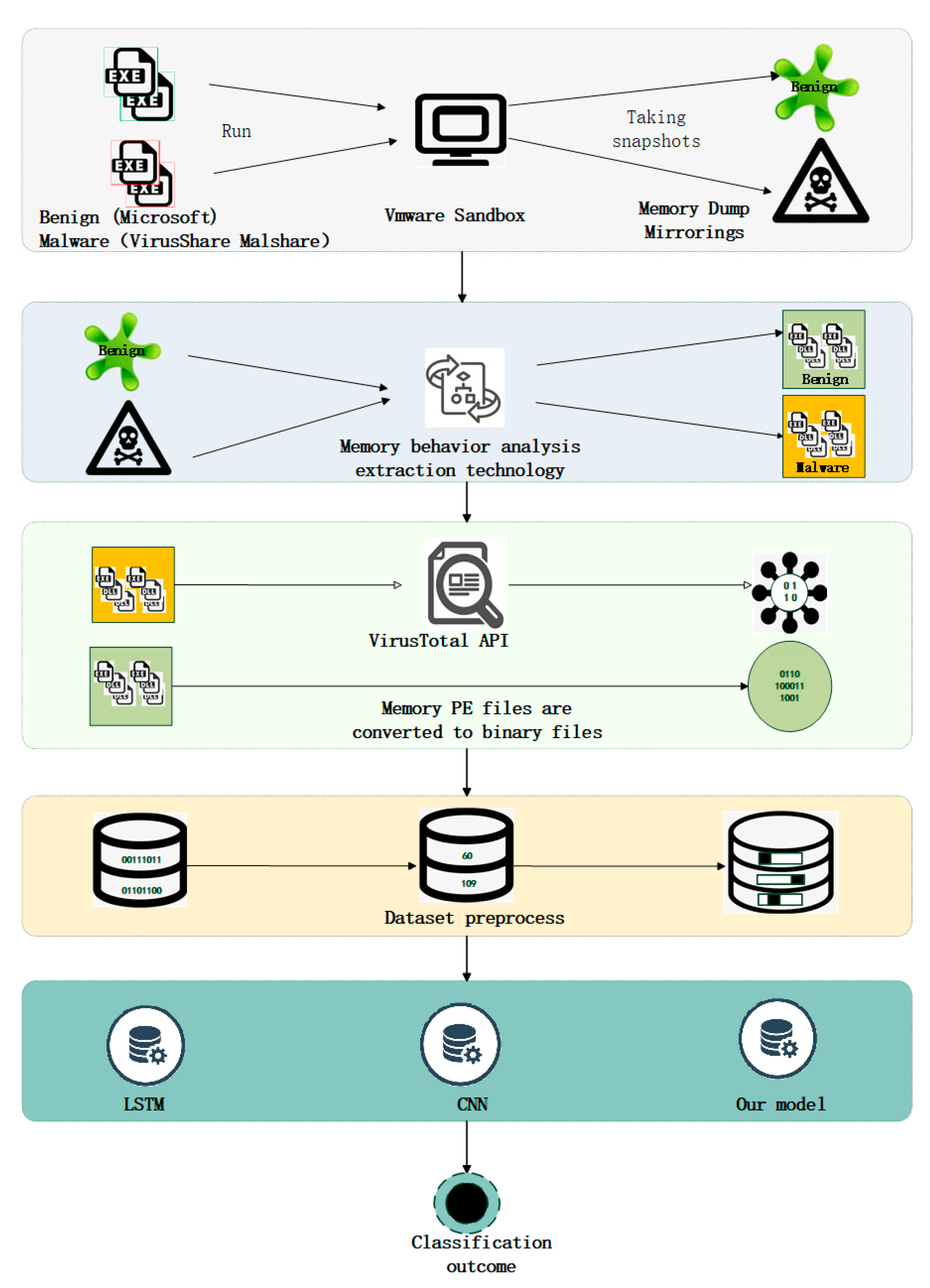
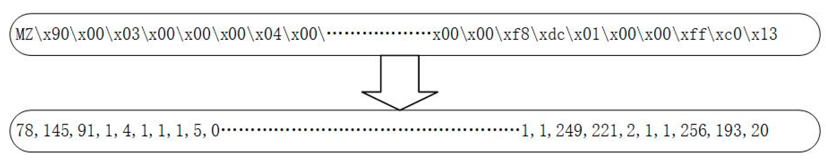
With regards to research on dynamic data, Wei [27] used KDD99 for experiments, multiple studies [28,29] used the kernel structure as the dataset for dynamic detection, and another study [5] used the binary file extracted from a single process to convert it into an image for the analysis. The process-related DLL files were not exploited yet. To maximize the malicious files in the memory, we extract all process and DLL files from the memory dump and created a dataset.

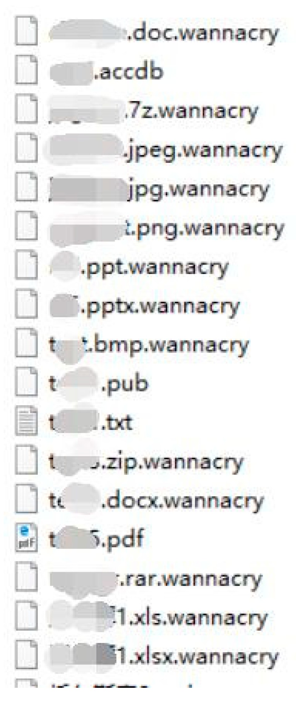
First of all, the common softwares (office, video, audio, and games et.) in the Windows system are downloaded. Then the softwares are executed and the memory process files are dumped. Mostly, memory dump files are dumped every 10 min and the operation is repeated ten times. PE files are dumped multiple times because the software does not load all files into memory at runtime. To collect malicious samples, static malicious PE files are downloaded from the VirusShare and Malshare malicious code, libraries which are widely used by researchers [30,31], and then malicious samples are executed in virtual machines. The extraction method of dynamic malicious samples is the same as that of benign samples. Malicious samples are dumped at a certain interval.

Finally, a total of 4896 data samples are obtained. To identify whether the extracted samples are benign or malicious samples, the benign and malicious samples are authenticated through the API interface of VirusTotal.

4.2. Dataset Preprocessing

4.2.1. Data Type Conversion

The dataset of the memory file is considerably different from the text dataset of natural language processing. We first preprocess the dataset by using natural language word segmentation; that is, by converting binary data into single words and then conducting word embedding. However, when the model is used to train the processed samples, the training result is inferior, with an accuracy of approximately 0.5, which is of no value for dichotomy classification. After conducting research, it is found that the memory PE binary file has many consecutive 0 s appearing in the file, which cannot be effectively learned for the data after the word segmentation. Several studies [9,32] converted the binary data into images as datasets. A previous study [14] directly learned the binary files during data preprocessing. Figure 3 shows our operations on the data type transformation of the dataset. The value range of the 8-bit binary number is 0–255, and the value of the image is also 0–255. Since convolutional neural networks perform well in image classification, we convert every eight binary bits of the malicious code to a decimal, making it a similar form to image numerical values. The training data should be cut to the same length before being added to the training model. We first add 1 to the data in the dataset, and then for data more minor than the length, 0 is used to fill in the data to avoid mixing with the actual data.

4.2.2. Segment Selection

The dataset sample takes a fragment of the sample for training. Three methods are adopted to intercept part of the data in the sample.

• As is shown in Figure 4, the sample header is selected for fragmentation, and the lengths of the header for the fragmentation are 32, 64, 128, 256, 512, 1024, 2048, 4096, 10,000, and 30,000 bytes. The effect of taking different lengths of the sample fragments on the model’s accuracy is observed through experiments. Additionally, the method of sample fragment training can also improve the detection efficiency of the model and significantly reduce the time taken for sample detection;

• As is shown in Figure 5, the tail of the sample is selected for the fragmentation such that the influence of the different positions of the fragment on the training accuracy can be judged. The tail is chosen to extract the sample fragment, and the extracted length is the same as the length extracted from the header, so the effect of the different positions can be better performed;

• As is shown in Figure 6, samples for the fragmentation are selected randomly. To better reflect the influence of the different locations on the experimental results, samples with the same fragment length but other locations are randomly extracted for each sample.

4.3. Our Model

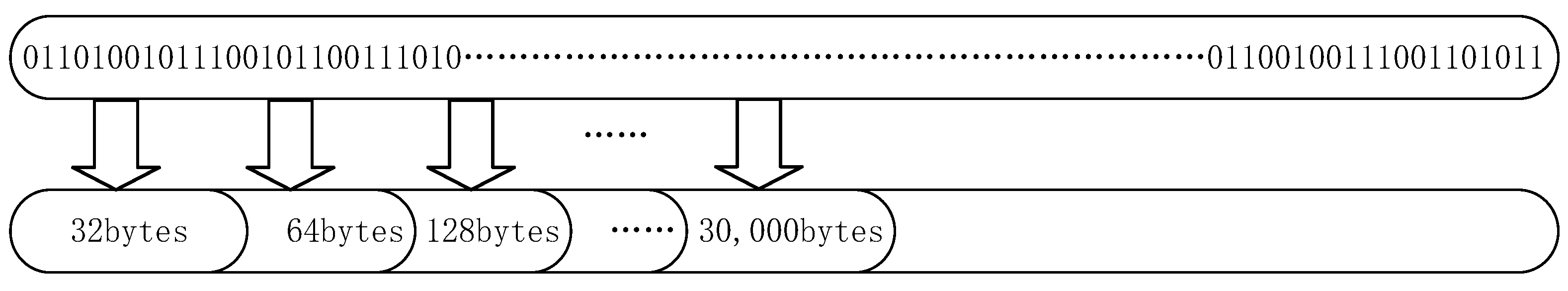
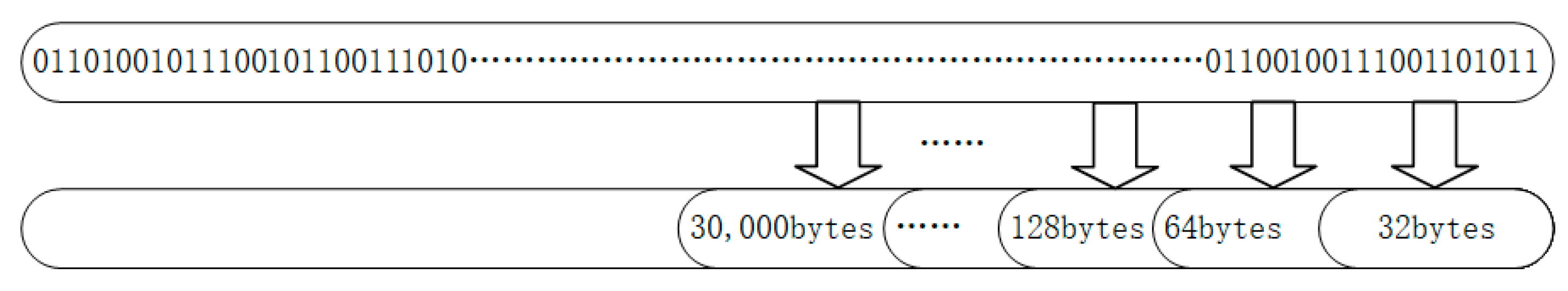
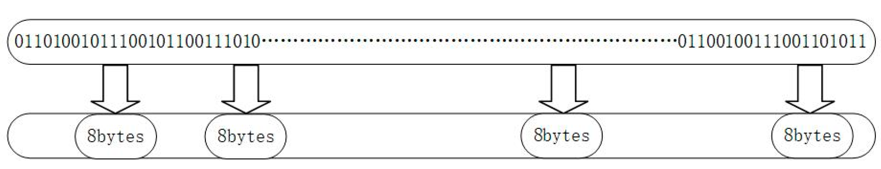
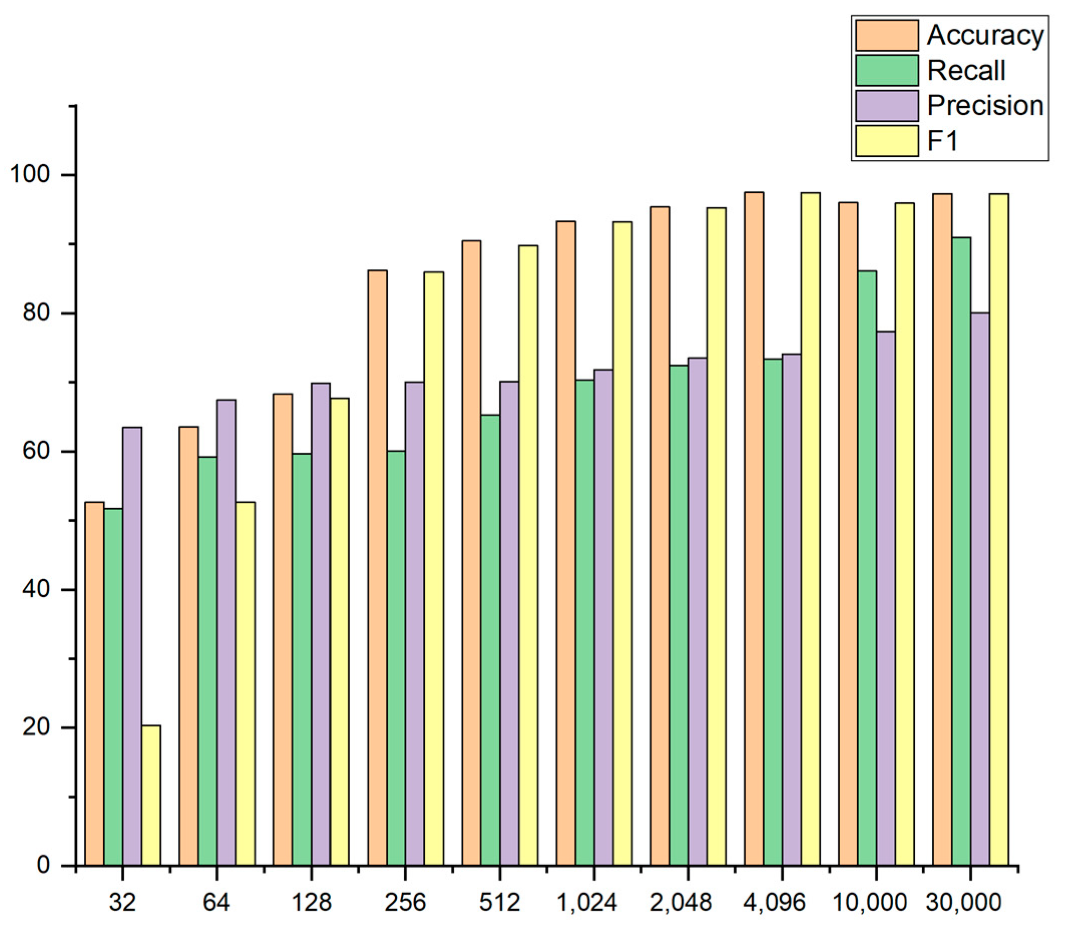
To address the problems that the dynamic PE files are incomplete and professional detection of malware is difficult, a deep model framework is proposed to learn the characteristics of the dynamic PE files to achieve the purpose of classification. The tiny fragment of the memory PE files (256 bytes) exhibits good detection results.

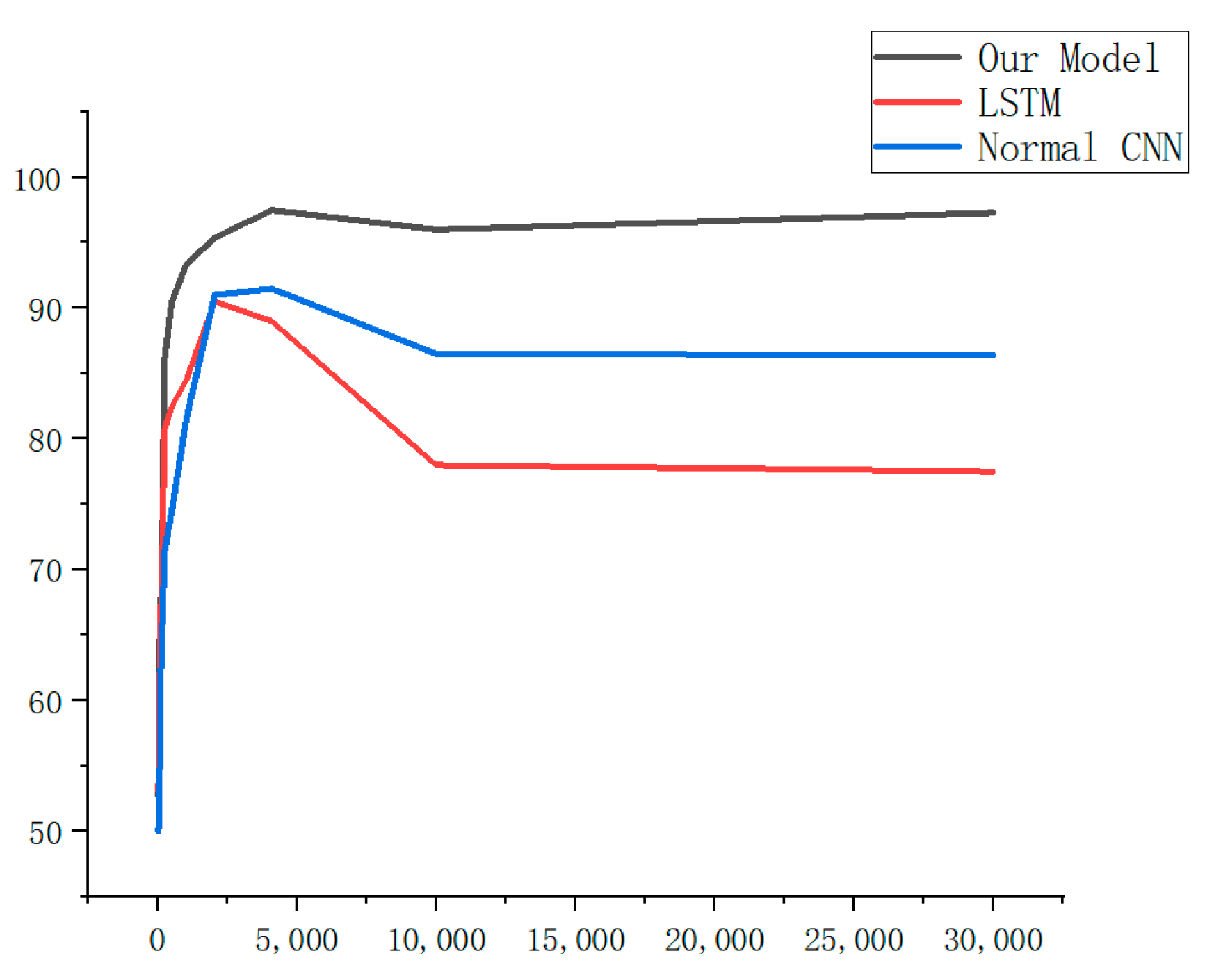
In the selection process of the deep learning model, long short-term memory [33] (LSTM) is firstly used for the experiments. LSTM is relatively mature in the field of natural language processing [34,35,36]. However, the experimental results show that the time cost of model training is higher than that for CNN. 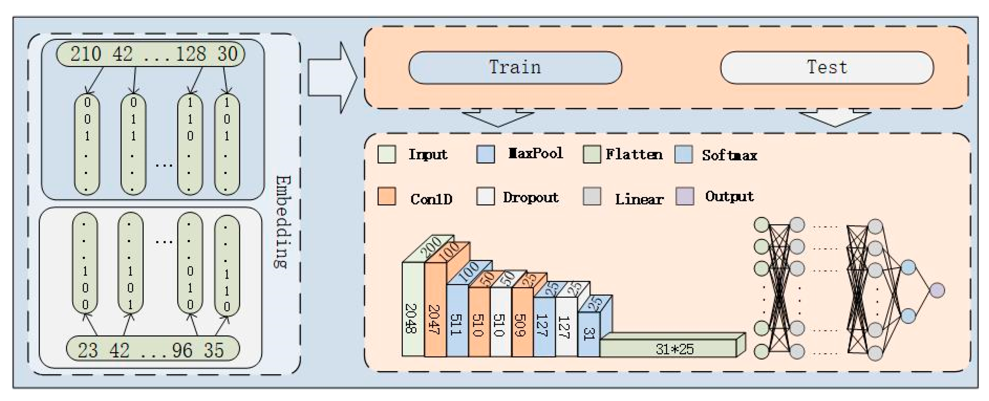Owing to the complex and diverse forms of malicious code, the features extracted by the CNN have translation invariance characteristics [37]. As the location of malicious code is not fixed, CNN is more suitable for the malicious code detection in binary PE files. In addition, with the increasing length of sequence fragments, the computation amount of the LSTM model will be very large and the procedure is time-consuming. Although the training duration of the ordinary CNN model is shorter than that of the LSTM, the training effect of CNN is similar to that of LSTM in terms of accuracy. Our model architecture is designed to maximize learning from preprocessed samples, as shown in Figure 7. We adopted a network model with a 12-layer structure based on CNN, in which we primarily used multiple convolutional layers for the model’s architecture. To prevent overfitting of the model during training, we added multiple dropout layers. The general dropout layer hides a quarter of the neuron nodes. In the study that proposed the famous VGG structure, Simonyan and Zisserman [21] observed that for a given receiving field, the performance of the stacked small convolutional kernel is better than that of the large convolutional kernel because multiple nonlinear layers can increase the network depth. Hence, the convolution kernels used in this study are small. For the optimizer in deep learning, the accuracy rate of Adam was found to be better than that of the SGD. Therefore, Adam was adopted, and a cross-entropy loss function was adopted for the loss function of deep learning back propagation. The pre-processed dataset in Section 4.2 is one-dimensional data, so the one-dimensional convolutional neural network (CNN1D) is adopted in our model. The difference between CNN1D and CNN is that CNN is mainly used for the detection of two-dimensional images, while CNN1D is used for the detection of one-dimensional data. We use CNN1D to input one-dimensional data into the model with a multi-channel mode, and then we do continuous translation calculation by the convolution kernel. The tag values are compared by using the softmax function. Finally, the cross entropy loss function is used for back propagation to optimize the model; thus, achieving the accurate detection of malicious code detection can be achieved with high accuracy. The processing procedure of LSTM model is similar to the above method. The preprocessed one-dimensional data are also input to the LSTM model for training and malicious code detection can be realized.

4.4. Neural Network Algorithm

This section introduces the algorithm in the neural network model designed for this study.

The output characteristics of the first, second, and third convolution layers in the PyTorch environment can be expressed as:

$$out\left(N_i,C_{ou{t}_j}\right)=bias\left(C_{ou{t}_j},k\right)+{\displaystyle \sum }_{k=0}^{C_{in}-1}weight\left(C_{ou{t}_j},k\right)\times input\left(N_i,k\right)$$

(1)

where N is the batch size, C is the channel size, L is the sequence length, and bias is the offset value of the neural network. Batch refers to the number of samples processed in batches, as the samples are divided into several groups. The number of samples in each group is the size of the batch, i is the index of the sample groups, j is the index of the number of samples, and k is the index of the input channel.

The length of the output sequence comprising the first, second, and third convolution layers is calculated using the following equation:

$$L_{out}=\lfloor \frac{L_{in}+2\times padding-dilation\left(kernel\_size-1\right)-1}{stride}+1\rfloor$$

(2)

where L_out is the output sequence length, L_in is the length of the input sequence, padding is the filling length, dilation is the size of the cavity convolution, which is set to 1, kernel_size is the size of the convolution kernel, and stride is the size of the step.

The input parameters of the flatten layer are computed using the output parameters of the pooling layer. The sequence is flattened using a flattened layer, then transformed into two neuron nodes by a fully connected layer, and finally classified by a softmax function.

The softmax layer, which is the last layer of the hidden layer, namely the classifier, is expressed as:

$$y_k=\frac{exp\left(a_k\right)}{{{\displaystyle \sum }}_{i=1}^{n}exp\left(a_i\right)}$$

(3)

The exp (x) denotes the exponential function of ex (e is the Napier’s constant = 2.7182...), n represents the total number of neurons in the output layer, and y_k represents the output of the k neurons in the output layer, where the numerator is the exponential function of input signal a_k of the k neuron, and the denominator is the sum of the exponential functions of all input signals.

The loss function of the neural network model adopts the min-batch cross-entropy loss function:

$$E=-\frac{1}{M}{\displaystyle \sum }_m{\displaystyle \sum }_k t_{mk}log y_{mk}$$

(4)

where M represents the number of training set samples, t_mk represents the value of the k element of the m prediction sample, y_mk is the neural network’s output to the m prediction sample, and t_mk is the supervised data. By extending the loss function of a single piece of data to M pieces of data and dividing by M at the end, the average loss function of a single prediction fragment can be obtained. A unified indicator independent of the training data can be obtained through such averaging.

Through Equations (1) and (2), we can calculate each convolutional layer’s input and output sizes. In our model, the input parameters of the fully connected layer need to be manually calculated when training sample segments of different sizes. Calculating each layer’s length is complicated through the above formula. By observing and calculating the neural network model we constructed, we obtained the formula for calculating the input length of the fully connected layer in our model:

$$Flatte{n}_{in}=\frac{\left(\frac{\left(sampl{e}_{len}-1\right)}{maxpoo{l}_{size}}\right)-2}{maxpoo{l}_{size}{}^2}$$

(5)

Faltten_in represents the input length of the fully connected layer, sample_len represents the input sample length, maxpool_size means the size of the pooling layer, and conv_channel represents the output channel size of the last convolutional layer. Taking the fragment length of 2048 as an example, only the convolution layer and the pooling layer affect the data size, and the other neural network layers before the fully connected layer do not affect the data size. Our model has three convolution layers and three pooling layers, and the convolution kernel sizes of the three convolution layers are 3, 4, and 5, respectively. The maximum pooling is used for the pooling layer, and the three pooling layers are all set to 4. In our model, the padding of the convolution layer is set to 0, so the data length will be reduced by 1 after each convolution. It shrinks by a factor of four with each pooling. The order of convolution pooling in our model is convolution, pooling, convolution, convolution, pooling, and pooling; after the convolution pooling of our model, the length of the data with a sample fragment length of 2048 is firstly reduced by 1, and then the length is reduced by four times. By subtracting the output of the previous layer by 1 twice, and twice reducing it by four times, the sample length becomes 31. Finally, multiplying 31 by the number of output channels of the last convolutional layer is the input parameter of the fully connected layer. Figure 7 shows the detailed calculation process of the input length of the flattening layer in the neural network section.

The detailed parameter settings of the neural network model are introduced in the Section 5.3.

5. Experimental Overview

5.1. Operating Environment and Datasets

The hardware CPU of our experiment is the Intel(R) Core(TM) i7-11800H processor, configured with two 8G memory; NVIDIA GeForce RTX 3050 graphics card. The software environment is a 64-bit Windows10 operating system and VMWare, which installs Windows 7 and Windows XP virtual machines to run malicious samples. The environment for building and running the deep learning framework is Python 3.7, Anaconda conda 4.11.0, and PyTorch torch1.10.1. The dataset is generated as follows: collecting static samples from VirusShare and Malshare, running the samples in the virtual machine, dumping memory information and extracting processes, and DLL files from the memory data.

5.2. Evaluation Metrics

For detecting malicious code, we use the four evaluation indexes of binary classification: accuracy, precision, F-measure, and recall [38]. F-measure implies that one index can reflect both the accuracy and recall rates.

$$recall=TP/\left(TN+FN\right)$$

(6)

$$Precision=TP/\left(TN+FP\right)$$

(7)

$$F-measure=2\times \left(Precision\times recall\right)/\left(Precision+recall\right)$$

(8)

$$Accuracy=\left(TP+TN\right)/\left(TP+FP+TN+FN\right).$$

(9)

TP represents the number of samples that are predicted to be malicious samples out of the genuinely malicious samples. FP represents the number of truly benign samples predicted to be malicious samples. TN represents the number of genuinely benign samples that are predicted to be benign samples. FN indicates that the actual sample is malicious and the predicted sample is benign.

5.3. Datasets Parameter Optimization

When the segment length is less than 1024 bytes because the proposed model undergoes multiple convolutions and pooling, the length of the last convolutional layer is greater than the output sequence length of the previous network layer, and the model cannot be trained.

Table 1. Model convolution pooling size for parameter tuning.

Fragment Length [Byte]	Convolution Kernel 1	Max Pool	Convolution Kernel 2	Convolution Kernel 3
32	5	2	3	2
64	3	2	4	5
128	3	2	4	5
256	3	3	4	5
512	3	4	4	5
1024	3	4	4	5

lists the adjusted parameters of the convolution and pooling layers of the model for the cases in the experiment when the length is less than 1024. Subsequently, the optimal parameters suitable for the current length are obtained. When the fragment length is larger than 1024, parameters of the convolution and pooling layers for a length size of 1024 are adopted.

5.4. Sample Fragments of Different Lengths

As demonstrated through the results presented in

Table 2. Sample fragments of different lengths.

Fragment Length	Accuracy	Recall	Precision	F-Measure
32	52.67	11.34	83.45	20.38
64	63.58	39.5	78.99	52.66
128	68.28	66.39	69.00	67.67
256	86.21	84.03	87.85	86.02
512	90.43	84.12	96.28	89.79
1024	93.34	89.91	96.83	93.24
2048	95.38	93.28	97.97	95.28
4096	97.48	96.22	98.71	97.45
10,000	96.00	94.11	97.81	95.93
30,000	97.27	97.90	96.68	97.29

, when our model detects data samples of different lengths for training, the strategy is to select the intercepted fragments from the header.

As shown in Figure 8, the training model performs poorly, and no effective features are extracted when the fragment length is 32. When the fragment length is 256, the training accuracy is improved, and all evaluation indices are stable. As the length of the training segment increases, the accuracy rate improves, and the accuracy rate reaches the maximum value when the size is 4096. By training samples of different lengths, detecting malicious samples can be enhanced by detecting fragments of samples.

5.5. Sample Fragments of Different Lengths

The influence of different sampling locations on the experimental results is investigated to explore the change in the accuracy of different locations of the same sample upon sampling the same length. For the location selection of sample fragments, we extracted samples from the head, the tail, and randomly, as demonstrated in

Table 3. Sample fragments from different locations.

Fragment Length	Extraction Head	Extraction Tail	Random Extraction
32	52.67	51.72	63.50
64	63.58	59.24	67.46
128	68.28	59.66	69.90
256	86.21	60.08	70.07
512	90.47	65.27	70.12
1024	93.34	70.37	71.79
2048	95.38	72.43	73.52
4096	97.48	73.38	74.09
10,000	96.00	86.13	77.31
30,000	97.27	90.97	80.04

. In the process of random extraction, each sample location was random, which increased the difficulty of sample extraction.

As seen from Figure 9, when the sample is sampled at the head, the prediction accuracy of the model is the highest, and the head has more features because the head contains the most critical feature information. The accuracy of tail extraction is the lowest, indicating that the tail includes the least number of key features. This is because only the critical data are called in the memory when the sample runs. Additionally, owing to the page replacement mechanism of the memory, as the system runs for a longer time, pages are constantly swapped into the memory, and pages existing in the memory are also temporarily swapped out, resulting in the least number of data features in the tail of the sample. Although random extraction is random for the location of different samples, it exhibits good accuracy. Furthermore, when the length of training data is greater than 10,000, the accuracy of tail extraction is high.

5.6. Comparison of Different Models

To verify the advantages of the proposed model, we perform comparative experiments with the common deep learning model LSTM and CNN.

Table 4. Comparison of different models.

Fragment Length	Our Model	LSTM	Normal CNN
32	52.67	52.99	50.00
64	63.58	60.49	52.36
128	68.28	67.99	63.46
256	86.21	80.75	71.45
512	90.47	82.47	74.50
1024	93.34	84.49	81.49
2048	95.38	90.50	90.99
4096	97.48	88.99	91.49
10,000	96.00	77.99	86.50
30,000	97.27	77.49	86.37

lists the results of the comparison. Additionally, we conduct several experiments on these models and find out the optimal results. Extensive experiments show that the proposed model outperforms the compared models. In particular, the longer the sample sequence, the longer the time to train the LSTM. For the same sequence length, the proposed model takes 6 h to train, while the LSTM takes 30 h, and the training effect is less accurate than that of the proposed model. There is a negligible difference between the ordinary CNN training and research training time. Figure 10 illustrates that the proposed model is superior in terms of accuracy.

We also compared commonly used machine learning methods. We converted binary files in our dataset into gray images, then used HOG for feature extraction, and finally used standard machine learning methods XGB, light gradient boosting machine (LGBM), random forest (RF), SVM, decision tree, and deep forest (DF) for detection. As shown in

Table 5. Comparison of different models.

Machine Learning Model	Image Width (Pixels)	Accuracy	Recall	Precision	F-Measure
XGB 1	32	87.44	88.66	87.44	88.01
LGBM 2	32	87.44	88.72	87.44	88.03
RF 3	32	89.82	93.34	89.82	91.50
Decision tree	32	83.85	74.01	83.85	78.42
SVM 4	32	69.60	60.05	69.60	63.90
DF 5	32	92.81	97.91	88.94	93.17
XGB	64	87.44	88.66	87.44	88.01
LGBM	64	87.44	88.72	87.44	88.03
RF	64	89.82	93.34	89.82	91.50
Decision tree	64	83.85	74.01	83.85	78.42
SVM	64	69.60	60.05	69.60	63.90
DF	64	92.81	97.91	88.94	93.17
XGB	128	87.44	88.66	87.44	88.01
LGBM	128	87.44	88.72	87.44	88.03
RF	128	89.82	93.34	89.82	91.50
Decision tree	128	83.85	74.01	83.85	78.42
SVM	128	69.60	60.05	69.60	63.90
DF	128	92.81	97.91	88.94	93.17
XGB	256	87.44	88.66	87.44	88.01
LGBM	256	87.44	88.72	87.44	88.03
RF	256	89.82	93.34	89.82	91.50
Decision tree	256	83.85	74.01	83.85	78.42
SVM	256	69.60	60.05	69.60	63.90
DF	256	92.81	97.91	88.94	93.17

¹ XGBoost, ² LightGBM, ³ Random Forest, ⁴ Support Vector Machine, ⁵ Decision Forest.

, we transform binary files into grayscale images with four different pixels, which are detected by the above six machine learning methods.

Figure 11 shows the best performance accuracy of the machine learning methods in Table 2. Different machine learning methods also have obvious differences. Among them, decision tree has the worst performance on our dataset, and DF has the best performance, but our model still has high accuracy.

We not only compare common machine learning and deep learning methods, but also reproduced the technologies used in [9,12,17] and in related work using our dataset and compared them.

Table 6. Comparison of different models.

Study	Accuracy	Recall	Precision	F-Measure
Bozkir et al., 2021 [5]	93.44	96.23	91.20	93.60
Lu XD et al., 2020 [18]	94.73	97.49	92.77	95.03
Huhua Li et al., 2019 [13]	91.94	82.91	99.76	90.65
Our Model	97.48	96.22	98.71	97.45

clearly shows the four measurement indicators, and our performance is better than theirs.

5.7. Example of Fileless Malware Detection

A fileless attack spreads over the network, and no trace of the virus can be detected on the local disk because such an attack does not store files on the disk. Many fileless attacks are sent to your computer through emails, and when you click to view them, your computer will be attacked. The Bitcoin ransomware virus swept the world in 2017, and we analyzed it in a similar sample recently. The sample attack can be discovered by analyzing processes, threads, registries, and other behaviors. When the sample is executed, it does not create a separate process but injects its malicious program into cmd.exe. It is difficult to find this type of ransomware. After the sample is executed, it encrypts our files, which must be decrypted by paying for bitcoins. The suffix of the sample is .docx.exe. Imagine if the suffix of the file is hidden and spread by email, will many people click on the file?

We first create a clean system in the virtual machine, run the cmd window, open the virtual host monitor, see that the cmd process already exists, dump the virtual system, and extract a single cmd file named 1.bytes. We run the prepared malicious code sample in the virtual machine and check the running status of the virus sample. The virus sample, after running, encrypts Doc, Docx, Xls, xlsx, ppt, pptx, BMP, jpg, png, jpeg, zip, 7z, and RAR files, and the process is not found in the process list. Figure 12 shows the encrypted file data for the virus sample.

We will dump the virtual machine that ran the sample and then extract a single cmd.exe file named 2.bytes. Using the model we trained and saved, we detect that 1. bytes files are benign and 2. bytes files are malicious. The file we dumped is shown in Figure 13, and Figure 14 is the result of the model output after our detection. Therefore, this type of attack cannot be detected in static files, and this malicious code can only be detected in dynamic analysis.

6. Summary and Future Prospect

We adopted a CNN-based neural network model to detect malicious code for fragments of memory PE files, trained sample fragments of different lengths and locations, and obtained conclusive experimental results. We believe our results have tremendous implications for memory forensics and malicious code detection.

• We create a dataset of in-memory PE files, which includes benign and malicious samples;
• For dynamic files, deep learning can effectively detect memory PE files containing malicious codes;
• The binary data samples can still perform satisfactorily without complicated pre-processing means and can accurately predict the data samples;
• Based on the comparison of the experimental data, the detection effect of the 4096-byte fragment is found to be the best. It is proved that dynamic PE files containing malicious codes can be detected by detecting fragments of the dynamic PE files, thus improving the efficiency of the memory forensics personnel.

In our model, the selected detection fragments may not contain malicious code if the malicious code does not run for a long time or does not run during the detection time. This possibility will enhance the false positives. In the future, we will focus on improving our model to detect and classify multi-families of dynamic malicious behaviors and adapt to enhance the model’s sustainability. We will also explore new methods to achieve an accurate selection of PE file fragments. Based on the results of this study, the detection of virtual machine escapes can be studied in the future.

References

1. Conti, M.; Khandhar, S.; Vinod, P. A few-shot malware classification approach for unknown family recognition using malware feature visualization. Comput. Secur. 2022, 122, 102887. [Google Scholar] [CrossRef]
2. Malware Statistics & Trends Report|AV-TEST. AV Test Malware Statistics. Available online: https://www.av-test.org/en/statistics/malware (accessed on 23 December 2022).
3. Greenstein, S. The Economics of Information Security and Privacy. J. Econ. Lit. 2014, 52, 1177–1178. [Google Scholar]
4. Khalid, O.; Ullah, S.; Ahmad, T.; Saeed, S.; Alabbad, D.A.; Aslam, M.; Buriro, A.; Ahmad, R. An Insight into the Machine-Learning-Based Fileless Malware Detection. Sensors 2023, 23, 612. [Google Scholar] [CrossRef] [PubMed]
5. Kara, I. Fileless malware threats: Recent advances, analysis approach through memory forensics and research challenges. Expert Syst. Appl. 2022, 214, 119133. [Google Scholar] [CrossRef]
6. Pradip, D.; Pradip, D.; Chakraborty, K. Advances in Number Theory and Applied Analysis; World Scientific: Singapore, 2023. [Google Scholar]
7. Franzen, F.; Holl, T.; Andreas, M.; Kirsch, J.; Grossklags, J. Katana: Robust, Automated, Binary-Only Forensic Analysis of Linux Memory Snapshots. In Proceedings of the 25th International Symposium on Research in Attacks, Intrusions and Defenses (RAID 2022), Limassol, Cyprus, 26–28 October 2022; ACM: New York, NY, USA 18p. [Google Scholar] [CrossRef]
8. Ligh, M.H.; Case, A.; Levy, J.; Walters, A. The Art of Memory Forensics: Detecting Malware and Threats in Windows, Linux, and Mac memory; John Wiley & Sons: Hoboken, NJ, USA, 2014. [Google Scholar]
9. Bozkir, A.S.; Tahillioglu, E.; Aydos, M.; Kara, I. Catch Them Alive: A Malware Detection Approach through Memory Forensics, Manifold Learning and Computer Vision. Comput. Secur. 2021, 103, 061102. [Google Scholar] [CrossRef]
10. Majd, A.; Vahidi-Asl, M.; Khalilian, A.; Poorsarvi-Tehrani, P.; Haghighi, H. SLDeep: Statement-level software defect prediction using deep-learning model on static code features. Expert Syst. Appl. 2020, 147, 113156. [Google Scholar] [CrossRef]
11. Jiang, F.; Cai, Q.; Lin, J.; Luo, B.; Guan, L.; Ma, Z. TF-BIV: Transparent and Fine-Grained Binary Integrity Verification in the Cloud. In Proceedings of the 35th Annual Computer Security Applications Conference, San Juan, PR, USA, 9–13 December 2019; pp. 57–69. [Google Scholar]
12. Zhang, Y.; Liu, Q.Z.; Li, T.; Wu, L.; Shi, C. Research and development of memory forensics. Ruan Jian Xue Bao/J. Softw. 2015, 26, 1151–1172. [Google Scholar]
13. Kawakoya, Y.; Shioji, E.; Otsuki, Y.; Iwamura, M.; Miyoshi, J. Stealth Loader: Trace-free Program Loading for Analysis Evasion. J. Inf. Process. 2018, 26, 673–686. [Google Scholar] [CrossRef]
14. Uroz, D.; Rodríguez, R.J. On Challenges in Verifying Trusted Executable Files in Memory Forensics. Forensic Sci. Int. Digit. Investig. 2020, 32, 300917. [Google Scholar] [CrossRef]
15. Cheng, Y.; Fu, X.; Du, X.; Luo, B.; Guizani, M. A lightweight live memory forensic approach based on hardware virtualization. Inf. Sci. 2017, 379, 23–41. [Google Scholar] [CrossRef]
16. Palutke, R.; Block, F.; Reichenberger, P.; Stripeika, D. Hiding process memory via anti-forensic techniques. Forensic Sci. Int. Digit. Investig. 2020, 33, 301012. [Google Scholar] [CrossRef]
17. Wang, L. Research on Online Forensics Model and Method Based on Physical Memory Analysis. Ph.D. Thesis, Shandong University, Jinan, China, 2014. [Google Scholar]
18. Raff, E.; Barker, J.; Sylvester, J.; Brandon, R.; Catanzaro, B.; Nicholas, C. Malware Detection by Eating a Whole Exe. In Proceedings of the Work-Shops at the Thirty-Second AAAI Conference on Artificial Intelligence, New Orleans, LA, USA, 2–7 February 2018. [Google Scholar]
19. Marín, G.; Caasas, P.; Capdehourat, G. Deepmal-deep learning models for malware traffic detection and classification. Data Sci. -Anal. Appl. 2021, 105–112. [Google Scholar]
20. Li, H.; Zhan, D.; Liu, T.; Ye, L. Using Deep-Learning-Based Memory Analysis for Malware Detection in Cloud. In Proceedings of the 2019 IEEE 16th International Conference on Mobile Ad Hoc and Sensor Systems Workshops (MASSW), Monterey, CA, USA, 4–7 November 2019; pp. 1–6. [Google Scholar]
21. Zhang, Y.; Li, B. Malicious Code Detection Based on Code Semantic Features. IEEE Access 2020, 8, 176728–176737. [Google Scholar] [CrossRef]
22. Wadkar, M.; Di Troia, F.; Stamp, M. Detecting malware evolution using support vector machines. Expert Syst. Appl. 2020, 143, 113022. [Google Scholar] [CrossRef]
23. Han, W.; Xue, J.; Wang, Y.; Liu, Z.; Kong, Z. MalInsight: A systematic profiling based malware detection framework. J. Netw. Comput. Appl. 2019, 125, 236–250. [Google Scholar] [CrossRef]
24. Huang, X.; Ma, L.; Yang, W.; Zhong, Y. A Method for Windows Malware Detection Based on Deep Learning. J. Signal Process. Syst. 2020, 93, 265–273. [Google Scholar] [CrossRef]
25. Lu, X.D.; Duan, Z.M.; Qian, Y.K.; Zhou, W. Malicious code classification method based on deep forest. Ruan Jian Xue Bao/J. Softw. 2020, 31, 1454–1464. [Google Scholar]
26. Simonyan, K.; Zisserman, A. Very deep convolutional networks for large-scale image recognition. arXiv 2014, arXiv:1409.1556. [Google Scholar]
27. Wei, Y.; Chow, K.P.; Yiu, S.M. Insider threat prediction based on unsupervised anomaly detection scheme for proactive forensic investigation. Forensic Sci. Int. Digit. Investig. 2021, 38, 301126. [Google Scholar] [CrossRef]
28. Le, H.V.; Ngo, Q.D. V-sandbox for dynamic analysis IoT botnet. IEEE Access 2020, 8, 145768–145786. [Google Scholar] [CrossRef]
29. Urooj, U.; Al-Rimy, B.A.S.; Zainal, A.; Ghaleb, F.A.; Rassam, M.A. Ransomware detection using the dynamic analysis and machine learning. Appl. Sci. 2021, 12, 172. [Google Scholar] [CrossRef]
30. Shree, R.; Shukla, A.K.; Pandey, R.P.; Shukla, V.; Bajpai, D. Memory forensic: Acquisition and analysis mechanism for operating systems. Mater. Today Proc. 2022, 51, 254–260. [Google Scholar] [CrossRef]
31. Jin, X.; Xing, X.; Elahi, H.; Wang, G.; Jiang, H. A Malware Detection Approach using Malware Images and Autoencoders. In Proceedings of the 2020 IEEE 17th International Conference on Mobile Ad Hoc and Sensor Systems (MASS), Virtual, 10–13 December 2020; pp. 1–6. [Google Scholar]
32. Singh, J.; Thakur, D.; Gera, T.; Shah, B.; Abuhmed, T.; Ali, F. Classification and analysis of android malware images using feature fusion technique. IEEE Access 2021, 9, 90102–90117. [Google Scholar] [CrossRef]
33. Xiao, X.; Zhang, S.; Mercaldo, F.; Hu, G.; Sangaiah, A.K. Android malware detection based on system call sequences and LSTM. Multimed. Tools Appl. 2019, 78, 3979–3999. [Google Scholar] [CrossRef]
34. Khalil, F.; Pipa, G. Is deep-learning and natural language processing transcending the financial forecasting? Investigation through lens of news analytic process. Comput. Econ. 2022, 60, 147–171. [Google Scholar] [CrossRef]
35. Ren, G.; Yu, K.; Xie, Z.; Liu, L.; Wang, P.; Zhang, W.; Wang, Y.; Wu, X. Differentiation of lumbar disc herniation and lumbar spinal stenosis using natural language processing–based machine learning based on positive symptoms. Neurosurg. Focus 2022, 52, E7. [Google Scholar] [CrossRef] [PubMed]
36. Jayasudha, J.; Thilagu, M. A Survey on Sentimental Analysis of Student Reviews Using Natural Language Processing (NLP) and Text Mining. In Proceedings of the Innovations in Intelligent Computing and Communication: First International Conference ICIICC 2022, Bhubaneswar, India, 16–17 December 2022. [Google Scholar]
37. Biscione, V.; Bowers, J.S. Convolutional neural networks are not invariant to translation, but they can learn to be. arXiv 2021, arXiv:2110.05861. [Google Scholar]
38. Ahmad, I.; Alqarni, M.A.; Almazroi, A.A.; Tariq, A. Experimental Evaluation of Clickbait Detection Using Machine Learning Models. Intell. Autom. Soft Comput. 2020, 26, 1335–1344. [Google Scholar] [CrossRef]
Figure 1. Process information analysis.
Symmetry 15 00758 g001
Figure 2. The overall workflow of the proposed approach.
Symmetry 15 00758 g002
Figure 3. Data type conversion.
Symmetry 15 00758 g003
Figure 4. Select head segment.
Symmetry 15 00758 g004
Figure 5. Select tail segment.
Symmetry 15 00758 g005
Figure 6. Select a random segment.
Symmetry 15 00758 g006
Figure 7. Our model.
Symmetry 15 00758 g007
Figure 8. Sample fragments of different lengths.
Symmetry 15 00758 g008
Figure 9. Sample fragments from different locations.
Symmetry 15 00758 g009
Figure 10. Comparison of different models.
Symmetry 15 00758 g010
Figure 11. Comparison of different models.
Symmetry 15 00758 g011
Figure 12. Encrypted file.
Symmetry 15 00758 g012
Figure 13. Detect file.
Symmetry 15 00758 g013
Figure 14. Detect result.
Symmetry 15 00758 g014