Comparing the Min–Max–Median/IQR Approach with the Min–Max Approach, Logistic Regression and XGBoost, Maximising the Youden Index

Abstract

Although linearly combining multiple variables can provide adequate diagnostic performance, certain algorithms have the limitation of being computationally demanding when the number of variables is sufficiently high. Liu et al. proposed the min–max approach that linearly combines the minimum and maximum values of biomarkers, which is computationally tractable and has been shown to be optimal in certain scenarios. We developed the Min–Max–Median/IQR algorithm under Youden index optimisation which, although more computationally intensive, is still approachable and includes more information. The aim of this work is to compare the performance of these algorithms with well-known Machine Learning algorithms, namely logistic regression and XGBoost, which have proven to be efficient in various fields of applications, particularly in the health sector. This comparison is performed on a wide range of different scenarios of simulated symmetric or asymmetric data, as well as on real clinical diagnosis data sets. The results provide useful information for binary classification problems of better algorithms in terms of performance depending on the scenario.

1. Introduction

The linear combination of multiple biomarkers is often used in clinical practice [1] for disease diagnosis due to its ease of interpretation and performance [2], which is usually superior to considering each biomarker separately [3,4,5,6,7,8]. These new biomarkers are key for disease screening or understanding the evolution of a disease after diagnosis. As an example, Prostate-specific antigen (PSA) is the most used biomarker to diagnose prostate cancer, although it lacks the necessary sensitivity and specificity. The prostate health index (PHI) and 4Kscore are new biomarkers with greater predictive ability derived from linear models that include PSA [9].

To assess diagnostic accuracy, statistics derived from the receiver operating characteristic (ROC) curve, such as the area under the ROC curve (AUC) [10] or the Youden index [11], are often used. In this context, the development of binary classification model approaches that maximise the AUC has been extensively studied in the literature. Many of these studies have been the basis for the formulation of subsequently published improved approaches under ROC-curve-derived optimality criteria.

Su and Liu [12] formulated the optimal linear model that maximises the AUC under the assumption of multivariate normality. This normality assumption is often not easy to observe in real clinical practice, being too demanding in part due to the symmetry that biomarkers must meet. For many diseases, the progression or advanced stages of them are associated with high values of the diagnostic tests, so these types of variables tend to follow asymmetric distributions. Results from a prostate cancer screening cohort show a clear asymmetry of PSA in the Canadian population [13]. This limitation was solved by Pepe et al. [14,15], who proposed a distribution-free approach for the estimation of the linear model that maximises AUC based on the Mann–Whitney U-statistic [16]. This approach is based on discrete optimisation under extensive search on the parameter vector of biomarkers coefficients. Although the statistical foundation underpinning the approach proposed by Pepe et al. has been the basis for subsequent approaches, it has the drawback of being computationally infeasible when the number of biomarkers is greater than or equal to three. To address this computational limitation, Pepe et al. [14,15] suggested the use of stepwise algorithms based on selecting and estimating, at each step, the best linear combination of two biomarkers, including at each step a new biomarker. This proposal for partial optimisations at each step was later implemented by Esteban et al. [17] and Kang et al. [18]. Esteban et al. included tie-handling strategies, and Kang et al. proposed a simpler and less demanding approach by setting the order of biomarker inclusion at the beginning of the algorithm. Liu et al. [19] proposed an approach, called the min–max approach, which is computationally tractable regardless of the number of biomarkers. This is because it is based on the linear combination of the minimum and maximum values of biomarkers under the optimisation of the Mann–Whitney U-statistic of the AUC, involving the search for a single optimal coefficient. Despite its computational advantage, it has been shown to generally achieve lower accuracy than other approaches that use information from all biomarkers, such as stepwise approaches, but shows superiority in some scenarios [3,4,18].

In diagnostic or binary classification problems where combinations of continuous biomarkers are estimated, dichotomisation of the resulting continuous value, i.e., establishing a cut-off point, is often key, as it provides a classification rule that allows this classification of patients into groups [20]. In this sense, the Youden index is a good criterion for choosing the best cut-off point to dichotomise a biomarker [21] and is an appropriate summary of the performance of the diagnostic model [22]. For example, the Youden index takes a cut-off value of 45.9 for PHI in nonfused biopsies [23]. The Youden index maximises the sum of sensitivity and specificity, giving equal weight to both metrics, so that it can be considered as the symmetrical point that maximises both metrics simultaneously.

Therefore, although there are different metrics that provide the optimal cut-off point, in the absence of consensus, with no clear reason to optimise either sensitivity or specificity, the Youden index provides that optimal balance, being the most used parameter to choose a threshold.

Although the area under the ROC curve is the most studied diagnostic assessment statistic in the literature, other statistics such as the Youden index are also used in different clinical studies and provide accurate categorisation. The algorithms under AUC optimality cited above were used as a basis for the formulation of subsequent approaches under Youden index maximisation. Based on the stepwise approach of Kang et al. [18], Yin and Tian [24] conducted a study under Youden index optimisation. Aznar-Gimeno et al. [25] developed the stepwise algorithm suggested by Pepe et al. [14,15] under Youden index maximisation and compared its performance with other approaches in the literature, modified under Youden index maximisation, such as Yin and Tian’s stepwise approach [24], the min–max approach [19], logistic regression [26], a parametric method with multivariate normality and a non-parametric kernel smoothing method. Although Aznar-Gimeno et al. demonstrated that their proposed approach achieved acceptable performance, superior in some scenarios, it has the computational limitation of being difficult to approach when the number of biomarkers increases. The min–max approach, which solves this computational problem through the linear combination of the minimum and maximum values, did not prove to be sufficient in terms of discrimination, except in a few specific scenarios.

Maintaining the advantage of not being subject to any distributional assumptions, being computationally tractable regardless of the number of original biomarkers while incorporating more information through a new summary statistic (the median or the interquartile range), Aznar-Gimeno et al. [27] proposed the so-called min–max–median and min–max-IQR approaches. These approaches are based on estimating the linear combination of these three variables using the proposed stepwise algorithm [25]. Aznar-Gimeno et al. compared the proposed algorithms with the min–max algorithm and logistic regression. The aim was to compare computationally tractable methods, regardless of the number of biomarkers. In this sense, cancer shows a substantial clinical heterogeneity, and the max–min derived approach tries to capture the potential variation underlying the biological heterogeneity.

Machine learning algorithms have been increasingly used in various fields of application [28] and, in particular, in clinical practice and medical research [29,30,31,32,33,34], due to their performance potential and efficiency. There are different machine learning and deep learning techniques that have been applied in the area of health from different sources of information covering different formats ranging from numerical data to text or images [35]. Numerous studies have applied and evaluated these techniques in recent years with different objectives in the healthcare domain [36], such as predicting events, diagnosing or prognosing diseases or cancers [37,38,39,40]. Analysing their association with patient biomarkers such as demographic data, clinical data, pharmacology, genetics, medical imaging or wearable sensors, [41] (among others), is a challenge that needs to be addressed in a way that prevents or detects the disease early.

Deep learning has been used to assist in the identification of genes and associated proteomics and metabolomics profiles to detect cancers at early stages [42,43,44]. Concerning the early detection of breast cancer, Mahesh et al. [45] evaluated the Naive Bayes classifier, the Decision Tree classifier, Random Forest and their ensembles. Botlagunta et al. [46] assessed nine machine learning methods for breast cancer metastasis classification, including logistic regression, k-nearest neighbours, decision trees, random forest, gradient boosting, and eXtreme Gradient Boosting (XGBoost) [47]. Rustam et al. [48] compared the performance of Support Vector Machine (SVM) and Naive Bayes for prostate cancer patient classification. Huo et al. [49] also evaluated the effectiveness of machine learning models for prostate cancer prediction, including SVM, decision tree, random forest, XGBoost, and adaptive boosting (Adaboost). Sabbagh et al. [50] applied logistic regression and XGBoost techniques to the prediction of lymph node metastasis in prostate cancer patients using clinicopathologic features. Khan et al. [51] propose a self-normalised multiview convolutional neural network model with adaptive boosting (AdaBoost-SNMV-CNN) for lung cancer nodule detection in computed tomography scans. Regarding diabetes, Saheb-Honar et al. [52] examined the classification ability of logistic regression, decision tree, and random forest in identifying the relationship between type 2 diabetes and its risk factors. Budholiya et al. [53] present a diagnostic system that employs an optimised XGBoost classifier with the aim of predicting the occurrence of heart disease. Ensemble models, combining machine learning and deep learning approaches, provide personalized patient treatment strategies based on medical histories and diagnostics [54]. The versatility of deep learning models is clear, with applications for omics data types, as well as histopathology-based genomic inference, providing perspectives on the integration of different data types to develop decision support tools [55], but few of them have yet demonstrated real-world medical utility [56].

The primary drawback of one of these algorithms compared to techniques based on linear models is the lack of explainability and interpretability of the models. One of the key reasons why these tools may not be effectively implemented and integrated into routine clinical practice is due to the lack of transparency and explainability of the models. Explainable artificial intelligence (XAI) is attracting much interest in medicine [57] and, fortunately, in recent years, work has been carried out on the concept of XAI, which provides techniques that also offer explainability and transparency of these models.

XGBoost [47] is one of the most widely used machine learning algorithms of recent times. This is due to its ease of implementation and good results, proving to be a leader in many competitions and state-of-the-art studies [58]. The XGBoost algorithm assumes no normality and combines several weak prediction models, which are usually decision trees, improving its predictivity and accuracy. This type of model shows versatility as it depends on some parameters relating to the building trees that can be optimized.

In terms of machine learning algorithms, our work focuses on analysing the predictive capacity of logistic regression and XGBoost. Numerous studies have compared the performance of logistic regression and XGBoost in the health domain in recent years [59,60,61,62,63,64,65,66]. Unlike logistic regression or other statistical approaches based on linear models, XGBoost allows capturing non-linear relationships, one of the main reasons for its popularity. However, although XGBoost is an effective tool in healthcare and has been in demand in recent years, demonstrating good performance, it does not always outperform conventional statistical methods such as logistic regression [62,66,67]. The choice of the optimal model will depend on the problem and the type of data. Therefore, it is always necessary to conduct a comprehensive comparative study to analyse the performance of algorithms in different scenarios in order to obtain useful information and establish certain guidelines.

Due to the enormous number of data available nowadays by the advances in technology, it has been shown that it is essential to develop non-parametric biomarker combination models that are computationally tractable, regardless of the number of initial biomarkers. In this sense, our proposed approaches (min–max–median/IQR approach) reduce the dimensional problem by capturing the heterogeneity of the information through summary statistics. Although studies comparing the performance of different machine learning techniques have increased in the literature in recent years, so far, there are no studies comparing the performance of our proposed approaches with machine learning models such as XGBoost, which has been in high demand in recent years and which can capture more complex relationships than the statistical linear methods compared in other studies [25,27]. The aim of our work was to compare the performance of our proposed min–max–median/IQR approaches with the min–max approach and the machine learning algorithms known as logistic regression and XGBoost, maximising the Youden index. For this purpose, they were compared on a wide range of simulated symmetric or asymmetric data scenarios, as well as on real clinical diagnostic datasets.

We provide a novel approach based on three main basic characteristics of the set of predictor variables, the maximum, minimum and median or IQR to capture the larger discrimination ability to summarize in these three parameters. On the other hand, from a different perspective, we train and validate additive tree models trying to capture the sum of the predictive ability of all predictor variables. The results of this work provide the reader with useful information that can serve as a guide for the choice of the most suitable algorithm for binary classification problems depending on the characteristics and behaviour of the data.

2. Materials and Methods

This section introduces some notations and the non-parametric approach of Pepe et al. [14,15], which forms the basis for our min–max–median/IQR approaches. In the following, we explain our proposed approaches (min–max–median/IQR) and the algorithms with which we compare performance: min–max approach, logistic regression and XGBoost. These algorithms were adapted by optimising the Youden index. Finally, the simulated scenarios and real datasets are detailed, as well as the validation procedure. The entire study was conducted using the free software R (The R Foundation for statistical computing, Vienna, Austria) [68]. The code of the whole study can be found in Supplementary Material.

2.1. Background

Consider the following binary classification problem where p is the number of biomarkers, $n_1$ is the number of case individuals (with disease) and $n_2$ is the number of control individuals (healthy individuals). If $X_{kij}$ denotes the value of the $j^{th}$ variable or biomarker ($j=1,\cdots ,p$) for the $i^{th}$ individual of group k = 1, 2 (disease and non-disease), then ${\mathbf{X}}_{\mathbf{ki}}$ is the vector of biomarkers for the $i^{th}$ individual of group k = 1, 2 and ${\mathbf{X}}_{\mathbf{1}}=\left({\mathbf{X}}_{\mathbf{11}},\cdots ,{\mathbf{X}}_{\mathbf{1}{\mathbf{n}}_{\mathbf{1}}}\right)$ and ${\mathbf{X}}_{\mathbf{2}}=\left({\mathbf{X}}_{\mathbf{21}},\cdots ,{\mathbf{X}}_{\mathbf{2}{\mathbf{n}}_{\mathbf{2}}}\right)$. Therefore, the linear combination of each group is expressed as ${\mathbf{Y}}_{\mathbf{k}}={\mathit{\beta }}^T{\mathbf{X}}_{\mathbf{k}},k=1,2$, where $\mathit{\beta }={({\beta }_1,\cdots ,{\beta }_p)}^T$ denotes the parameter vector.

Defined in the above notation, by definition, the Youden index (J) of the linear combination is expressed as:

$$\begin{array}{cc}\hfill J& =ma{x}_c\{Sensitivity\left(c\right)+Specificity\left(c\right)-1\}\hfill \\ \hfill & =ma{x}_c\{F_{{\mathbf{Y}}_{\mathbf{2}}}\left(c\right)-F_{{\mathbf{Y}}_{\mathbf{1}}}\left(c\right)\}\hfill \end{array}$$

(1)

where c denotes the cut-off point and $F_{{\mathbf{Y}}_{\mathbf{k}}}\left(c\right)=P({\mathbf{Y}}_{\mathbf{k}}\le c)$ the cumulative distribution function of random variable ${\mathbf{Y}}_{\mathbf{k}}$. Denoting by $c_{\mathit{\beta }}=\{c:ma{x}_c\left(F_{{\mathbf{Y}}_{\mathbf{2}}}\left(c\right)-F_{{\mathbf{Y}}_{\mathbf{1}}}\left(c\right)\right)\}$ the optimal cut-off point, the expression of the empirical estimate of the Youden index is:

$$\begin{array}{cc}\hfill {\widehat{J}}_{\mathit{\beta }}& ={\widehat{F}}_{{\mathbf{Y}}_{\mathbf{2}}}\left({\widehat{c}}_{\mathit{\beta }}\right)-{\widehat{F}}_{{\mathbf{Y}}_{\mathbf{1}}}\left({\widehat{c}}_{\mathit{\beta }}\right)\hfill \\ \hfill & =\frac{{\sum }_{i=1}^{n_2}I\left({\mathit{\beta }}^T{\mathbf{X}}_{\mathbf{2}\mathbf{i}}\le {\widehat{c}}_{\mathit{\beta }}\right)}{n_2}-\frac{{\sum }_{i=1}^{n_1}I\left({\mathit{\beta }}^T{\mathbf{X}}_{\mathbf{1}\mathbf{i}}\le {\widehat{c}}_{\mathit{\beta }}\right)}{n_1}\hfill \end{array}$$

(2)

where I denotes the indicator function.

Pepe et al.’s Approach

Pepe and Thompson [14] proposed a distribution-free approach (without any distribution assumptions) to estimate the linear model that maximizes the AUC based on the Mann–Whitney U-statistic [16]. The basis on which their proposed approach lies is mainly in the property of invariance of the ROC curve to any monotonic transformation.

Specifically, Pepe and Thompson propose the following linear model:

$$L_{\beta }\left(\mathbf{X}\right)=X_1+{\beta }_2{X}_2+\cdots +{\beta }_p{X}_p$$

(3)

where p denotes the number of biomarkers, $X_i$ the biomarker $i\in [1,\cdots ,p]$ and ${\beta }_i$ the parameter to be estimated. Observe that they did not include an intercept in the linear model (3), and the coefficient associated with the first variable $X_1$ is 1. This is because the ROC curves for $L_{\beta }\left(\mathbf{X}\right)$ (3) and $L_{\alpha }\left(\mathbf{X}\right)={\alpha }_0+{\alpha }_1{L}_{\beta }\left(\mathbf{X}\right),{\alpha }_1>0$ are the same, so it is enough to consider (3). Thus, considering the optimal parameter vector, the maximum empirical AUC based on the Mann–Whitney U statistic would be given by the following expression:

$$\widehat{AUC}=\frac{{\sum }_{i=1}^{n_1}{\sum }_{j=1}^{n_2}I(L_{\beta }\left({\mathbf{X}}_{\mathbf{1}\mathbf{i}}\right)>L_{\beta }\left({\mathbf{X}}_{\mathbf{2}\mathbf{j}}\right))+\frac{1}{2}I(L_{\beta }\left({\mathbf{X}}_{\mathbf{1}\mathbf{i}}\right)=L_{\beta }\left({\mathbf{X}}_{\mathbf{2}\mathbf{j}}\right))}{n_1·n_2}$$

Note that searching the entire possible parameter vector space ${\mathbb{R}}^{p-1}$ and possible coefficient-variable combinations is computationally intractable. To overcome this limitation, Pepe et al. suggested estimating the parameter vector through a discrete optimisation over 201 equally spaced values between −1 and 1. This is because selecting $\beta$ in $[-1,1]$ is equivalent to covering the range $(-\infty ,\infty )$ since the AUC of $X_i+\beta X_j$ for $\beta >1$ and $\beta <-1$ is the same as $\alpha X_i+X_j$ for $\alpha =\frac{1}{\beta }\in [-1,1]$. Even so, this optimisation is computationally costly for dimensions $p\ge 3$. To address this, Pepe et al. [14,15] suggested the use of stepwise algorithms, in which a new variable is included in each step, selecting the best combination of two variables. In this way, the problem is transformed into a computationally tractable problem by estimating a single parameter $p-1$ times using a linear combination of two variables.

Both the model formulation and the empirical search are the basis for the formulation of the min–max approach and our proposed algorithms (min–max–median/IQR) that extend the min–max approach, which are explained below.

2.2. Min–Max Approach

Liu et al. [19] proposed the so-called min–max approach (MM), which is a distribution-free approach, as proposed by Pepe et al. [14,15], but with the advantage of being computationally tractable, regardless of the number of original biomarkers. The idea of this approach is to calculate the minimum and maximum values of the p biomarkers and to consider the optimal linear combination of these two markers, involving the search for a single optimal coefficient. Specifically, the original aim is to estimate the $\beta$ parameter such as the combination

$$X_{min}+\beta X_{max}$$

(4)

which maximizes AUC based on the Mann–Whitney U statistic, where $X_{min}$ and $X_{max}$ are the minimum and maximum values of the original p biomarkers for each individual, respectively.

Considering the Youden index as our target metric to maximise, the min–max approach can be adapted by selecting the optimal parameter $\beta$ and cut-off point $c_{\beta }$ that maximises the following expression

$${\widehat{J}}_{\beta }=\frac{{\sum }_{i=1}^{n_2}I\left(X_{2i,max}+\beta X_{2i,min}\le {\widehat{c}}_{\beta }\right)}{n_2}-\frac{{\sum }_{i=1}^{n_1}I\left(X_{1i,max}+\beta X_{1i,min}\le {\widehat{c}}_{\beta }\right)}{n_1}$$

(5)

where $X_{ki,max}=ma{x}_{1\le j\le p}\left(X_{kij}\right)$ and $X_{ki,min}=mi{n}_{1\le j\le p}\left(X_{kij}\right)$ for $k=1,2$ and each $i=1,\cdots ,n_k$, and $\beta \in [-1,1]$, following Pepe et al’s. suggestion of the empirical search of $\beta$.

The procedure can be summarised as follows:

1.

For each i individual, the biomarkers with minimum and maximum values ($X_{min}$ and $X_{max}$) are considered as the new 2 markers (for simplicity, $X_1$ and $X_2$).

2.

For each of the 201 possible values of $\beta$, the value of the linear combination ($X_1+\beta X_2$) is calculated for each i individual and the optimal cut-off point is chosen, i.e., the one that maximises the Youden index.

3.

The linear combination that achieves the highest Youden index is the optimal combination.

2.3. Min–Max–Median/IQR Approach

Aznar-Gimeno et al. proposed new non-parametric approaches, so-called min–max–median (MMM) and min–max-IQR (MMIQR) [27], which extend the idea of the min–max approach by applying our proposed stepwise algorithm [25], following the suggestion of Pepe et al. [14,15]. The aim was to include more information in the model while remaining computationally affordable, although more intensive.

Specifically, the idea behind the approaches is to reduce the dimension of the problem by reducing the number of original p biomarkers to three, considering the summary statistic information of the original variables, i.e., the minimum, maximum, median, or interquartile range (IQR). Our approach extends the min–max approach as it incorporates a new summary statistic, turning the problem into a three-variable linear combination optimisation problem. As suggested by Pepe et al., a stepwise algorithm that we developed is used in this case, where the best linear combination of two variables is selected, including a new variable in each step.

Below, we provide a detailed description of the procedure for the min–max–median approach (note that the min–max-IQR approach follows the same steps).

1.

Firstly, for each i individual, the minimum, maximum, and median values of p biomarkers are calculated:

$$X_{ki,max}=\underset{1\le j\le p}{\max }\left(X_{kij}\right),X_{ki,min}=\underset{1\le j\le p}{\min }\left(X_{kij}\right),X_{ki,median}=media{n}_{1\le j\le p}\left(X_{kij}\right)$$

(6)

where $k=1,2$ and $i=1,\cdots ,n_k.$ These values are considered as the three new variables ($X_1$, $X_2$ and $X_3$, for simplicity). Specifically, from now on, the problem is to estimate the optimal linear combination of these three variables using the proposed stepwise algorithm.

2.

The first step of the stepwise approach is to choose the combination(s) of the two variables that maximises the Youden index such that

$${\widehat{J}}_{{\beta }_2}=\frac{{\sum }_{i=1}^{n_2}I\left(X_{2ij}+{\beta }_2{X}_{2ik}\le {\widehat{c}}_{{\beta }_2}\right)}{n_2}-\frac{{\sum }_{i=1}^{n_1}I\left(X_{1ij}+{\beta }_2{X}_{1ik}\le {\widehat{c}}_{{\beta }_2}\right)}{n_1}{\beta }_2\in [-1,1],\forall j\ne k=1,\cdots ,p$$

(7)

using empirical search proposed by Pepe et al. In other words, for each variable pair, for each value of the 201 ($\beta$ values), the linear combination is calculated and the optimal cut-off point that maximises the Youden index is selected. That linear combination for which the optimal cut-off point has obtained the maximum Youden index is chosen in this step. Suppose, for simplicity, the optimal linear combination $X_{ki1}+{\beta }_2{X}_{ki2}$.

3.

The last step is to include the remaining variable ($X_3$) and select the optimal linear combination(s). Specifically, the previously chosen linear combination ($X_{ki1}+{\beta }_2{X}_{ki2}$) is considered as a new variable and the idea of the previous point (2) is re-applied. Therefore, either combination (8) or (9) that maximizes the Youden index is chosen as the final optimal combination of the linear model.

$${\widehat{J}}_{{\beta }_3}=\frac{{\sum }_{i=1}^{n_2}I\left(\left(X_{2i1}+{\beta }_2{X}_{2i2}\right)+{\beta }_3{X}_{2i3}\le {\widehat{c}}_{{\beta }_3}\right)}{n_2}-\frac{{\sum }_{i=1}^{n_1}I\left(\left(X_{1i1}+{\beta }_2{X}_{1i2}\right)+{\beta }_3{X}_{1i3}\le {\widehat{c}}_{{\beta }_3}\right)}{n_1}{\beta }_3\in [-1,1]$$

(8)

$${\widehat{J}}_{{\beta }_3}=\frac{{\sum }_{i=1}^{n_2}I\left({\beta }_3\left(X_{2i1}+{\beta }_2{X}_{2i2}\right)+X_{2i3}\le {\widehat{c}}_{{\beta }_3}\right)}{n_2}-\frac{{\sum }_{i=1}^{n_1}I\left({\beta }_3\left(X_{1i1}+{\beta }_2{X}_{1i2}\right)+X_{1i3}\le {\widehat{c}}_{{\beta }_3}\right)}{n_1}{\beta }_3\in [-1,1]$$

(9)

For ease, a single optimal linear combination is considered in steps 2 and 3. However, the maximum Youden index can be reached for different linear combinations. Our algorithm considers all ties, which can be broken in the last stage (step 3) or not.

Our proposed approaches are openly available to the scientific community through the R library SLModels [69]. The library also incorporates the min–max algorithm adapted for the optimisation of the Youden index (previous section).

2.4. Logistic Regression

The logistic regression (LR) (or logit regression) [26] is a statistical model that provides the probability of an observation/individual i belonging to an output category, given its set of independent variables ${\mathbf{X}}_i$, through the logistics function:

$$\begin{array}{cc}\hfill P({\mathbf{Y}}_{\mathbf{i}}=1|{\mathbf{X}}_{\mathbf{i}})& =\frac{1}{1+e^{-{\mathit{\beta }}^T{\mathbf{X}}_{\mathbf{i}}}}=\frac{e^{{\mathit{\beta }}^T{\mathbf{X}}_{\mathbf{i}}}}{1+e^{{\mathit{\beta }}^T{\mathbf{X}}_{\mathbf{i}}}}\hfill \\ \hfill \log \frac{P({\mathbf{Y}}_{\mathbf{i}}=1|{\mathbf{X}}_{\mathbf{i}})}{1-P({\mathbf{Y}}_{\mathbf{i}}=1|{\mathbf{X}}_{\mathbf{i}})}& ={\mathit{\beta }}^T{\mathbf{X}}_{\mathbf{i}}\hfill \end{array}$$

(10)

where $\beta$ is the vector of parameters to estimate by means of the maximum likelihood method.

2.5. Extreme Gradient Boosting (XGBoost)

XGBoost (eXtreme Gradient Boosting, XGB) is a scalable tree boosting system that was developed by Chen and Guestrin [47]. It is a specific optimised implementation of gradient boosting and is therefore based on the principle of sequential order ensemble learning, where errors are minimized (loss function) using a gradient descent algorithm. Specifically, XGBoost is a decision tree ensemble based on the idea of training several weak learners (base learners) sequentially in order to create a strong learner with higher accuracy. During training, the parameters of each weak model are adjusted by minimising the objective function, and each new model is trained to correct the errors of the previous ones. Correctly and incorrectly predicted results receive different scores that are finally weighted to obtain a final result.

The XGBoost algorithm, unlike those presented above, has both parameters and hyperparameters. Hyperparameters are values of model settings that must be set during the training process to control the behaviour and performance of the model.

Considering the XGBoost algorithm as an ensemble base learners of decision trees, the loss function at iteration t to minimise has the following expression:

$$\begin{array}{c}\hfill {\mathcal{L}}^{\left(t\right)}=\sum _{i=1}^{n}l\left(y_i,{\widehat{y_i}}^{(t-1)}+f_t\left({\mathbf{X}}_i\right)\right)+\Omega \left(f_t\right)\end{array}$$

(11)

where l is the loss term and $\Omega \left(f\right)=\gamma T+\frac{1}{2}{\lambda \left|\right|\omega \left|\right|}^2$ is the regularisation term, which penalizes the complexity of the model, avoiding over-fitting. $y_i$ indicates the real output, ${\widehat{y_i}}^{(t-1)}$ the prediction of the $i^{th}$ individual at the ${(t-1)}^{th}$ iterations, f denotes the base learners, T the number of leaves of the tree and $\omega$ the weights of the leaves. $\gamma$ represents the minimum loss reductions needed to split a leaf node of the tree. The larger $\gamma$ is, the more conservative the algorithm will be.

The complexity of the model can also be limited through the maximum-depth hyperparameter, which specifies the maximum number of levels of the tree, where each level represents a division of the data based on a variable. Another possible regularisation hyperparameter is shrinkage, which reduces the step size to make the boosting process more conservative. In other words, it decreases the influence of each individual tree and allows future trees to improve the model. Random subsampling is another regularisation technique that can be used. In the case of a column subsample, the hyperparameter specifies the subsample fraction of columns to be used to construct each tree. The same idea is for rows, where, if the value is less than 1, a random subset of rows (observations/individuals) is selected for each tree.

The XGBoost model was applied using the free software R library xgboost. Specifically, in this study, the following hyperparameters were adjusted over a set of possibilities:

• nrounds: Number of decision trees in the final model.
• gamma ($\gamma$): Minimum loss reduction required to split a node.
• eta (shrinkage, learning rate): Step size shrinkage.
• max_depth: Maximum depth of the tree.
• colsample_bytree: Subsample ratio of columns.
• subsample: Subsample ratio of the training instances.

Table 1. Search space of the hyperparameters explored.

nrounds	gamma	eta	max_depth	colsample_bytree	subsample
50,100,200	0,0.5	0.1,0.3	[2,20]	0.5,1	0.5,1

shows the hyperparameter possibilities space explored in the study. The explored values of maximum tree depth for datasets with fewer variables were lower than those with higher dimensions. For the selection of the best combination of hyperparameters, the grid search technique was used, and 5-fold cross-validation was performed on the training set. Finally, the model was trained on the entire training dataset with the selected optimal hyperparameters. The early stopping technique was used as an additional technique to avoid over-fitting by stopping the training if there was no improvement in 10 iterations in a row.

2.6. Simulations

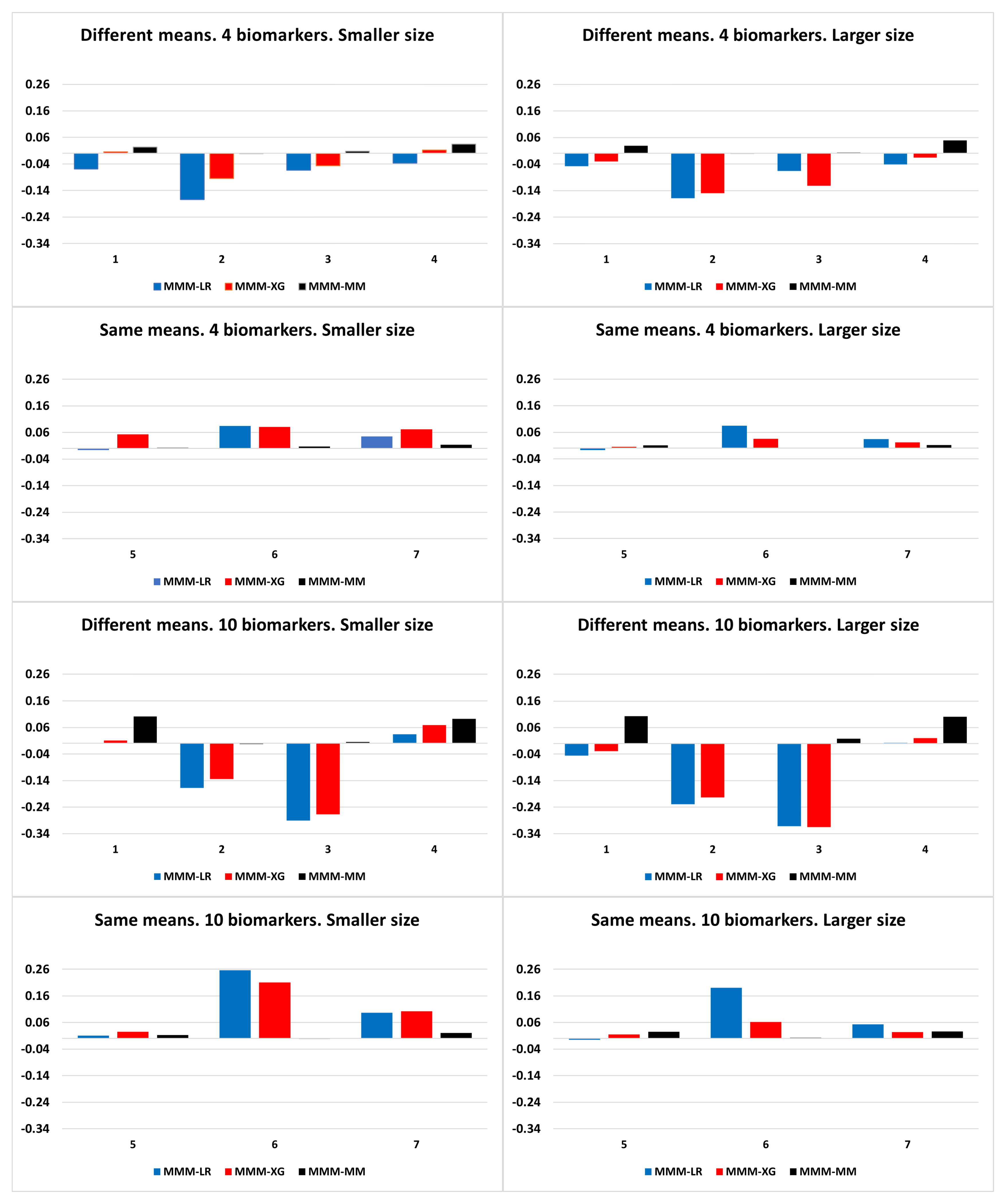
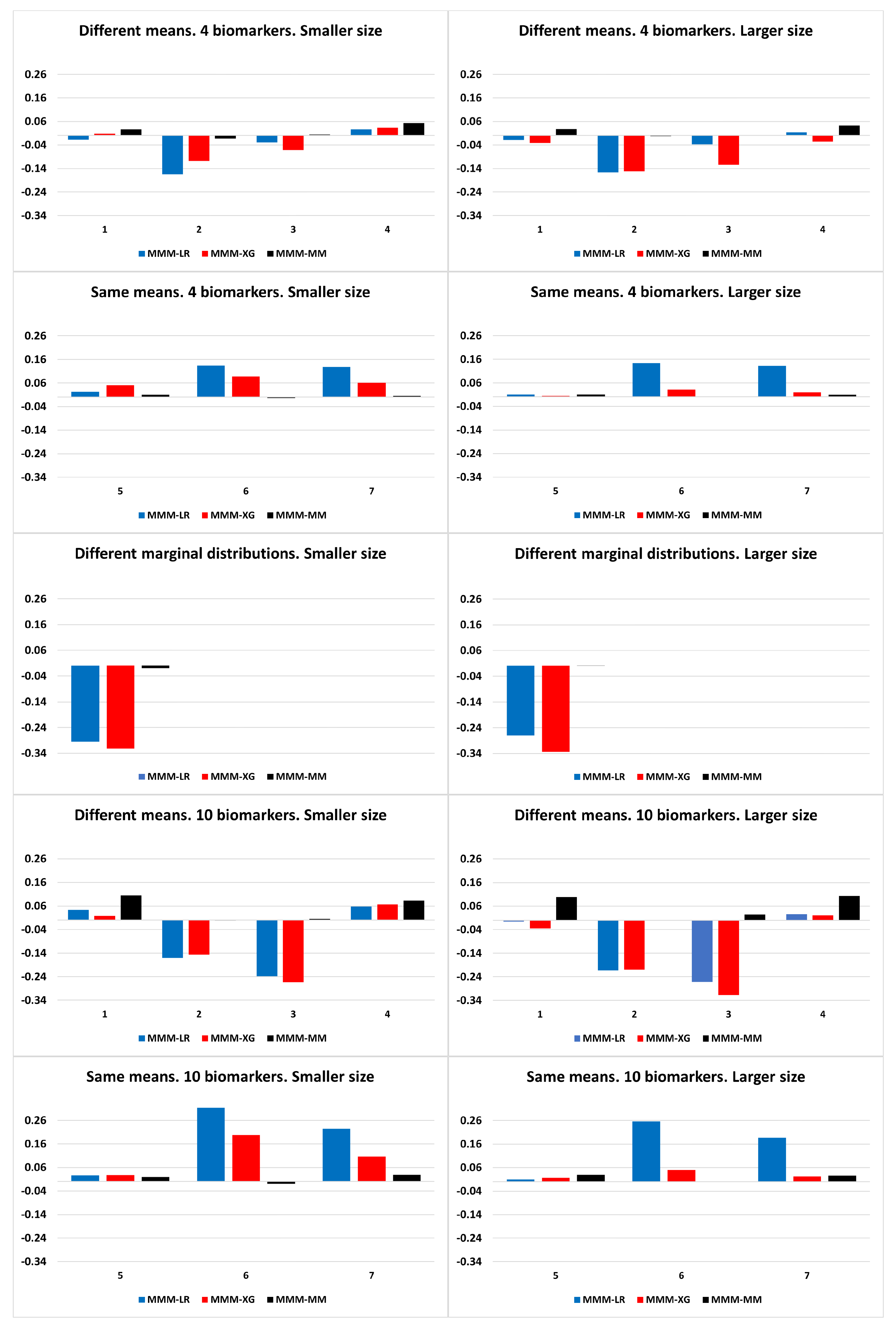
A wide range of simulated data were explored in order to analyse and compare the performance of the algorithms previously discussed. Specifically, scenarios simulating different biomarker distributions, discrimination capabilities, and correlation between them were analysed, considering $p=4$ and $p=10$ biomarkers, and smaller ($n_1=n_2$ = 50) and larger ($n_1=n_2$ = 500) sample sizes. As for the biomarker distributions, both symmetric distributions (normal distributions) and asymmetric distributions (different marginal distributions and multivariate log-normal skewed distribution) were simulated.

The scenarios with different marginal distributions were simulated with 4 biomarkers following chi-square, normal, gamma and exponential distributions via normal copula with a dependence parameter between biomarkers of 0.7 for the case population (patients; diseased population) and 0.3 for the control population (healthy; non-diseased population). More specifically, the biomarkers for the control population were considered to be marginally distributed as ${\chi }_{0.1}^2$, $N\left(0.1\right)$, $\Gamma \left(0.1\right)$, $Exp\left(0.1\right)$ and ${\chi }_{0.1}^2$, $N\left(0.6\right)$, $\Gamma \left(0.8\right)$, $Exp\left(0.1\right)$ for case population. Scenarios under log-normal distribution were generated from the configurations of the simulated scenarios under a normal distribution and then exponentiated.

Concerning the scenarios of normal distributions, the null vector $m_2=\overrightarrow{0}$ was considered as the mean vector of the non-diseased population. With respect to the mean vector of the diseased population ($m_1$), scenarios with the same means $m_1={(1.0,1.0,\cdots )}^T$, i.e., the same predictive ability, and different means $m_1={(0.2,0.5,1.0,0.7)}^T,m_1=(0.2,0.4,0.6,0.8,$${1.0,1.2,1.4,1.6,1.8,2.0)}^T$, were explored. For simplicity, the variance of each biomarker was set to 1, so that covariances are equivalent to correlations. The same correlation value was considered for all pairs of biomarkers. Let ${\Sigma }_1$ and ${\Sigma }_2$ be the variance–covariances matrices for diseased and non-diseased populations, respectively. The following scenarios with different biomarker means were analysed:

–

Independents (${\Sigma }_1={\Sigma }_2=I$).

–

High correlation (${\Sigma }_1={\Sigma }_2=0.3·I+0.7·J$).

–

Different correlation between groups (${\Sigma }_1=0.3·I+0.7·J,{\Sigma }_2=0.7·I+0.3·J$).

–

Negative correlation ($\rho =-0.1$).

• where I denotes the identity matrix and J the all-one matrix. Regarding scenarios with the same biomarker means, the following were explored:

–

Low correlation (${\Sigma }_1={\Sigma }_2=0.7·I+0.3·J$).

–

Different correlation between groups (${\Sigma }_1=0.3·I+0.7·J,{\Sigma }_2=0.7·I+0.3·J$).

–

Different correlation between groups with biomarkers independents in the non-diseased population (${\Sigma }_1=0.5·I+0.5·J,{\Sigma }_2=I$).

2.7. Application in Real Datasets

The methods being examined were also applied in two real clinical datasets: for the diagnosis of Duchenne muscular dystrophy and for maternal mortality risk.

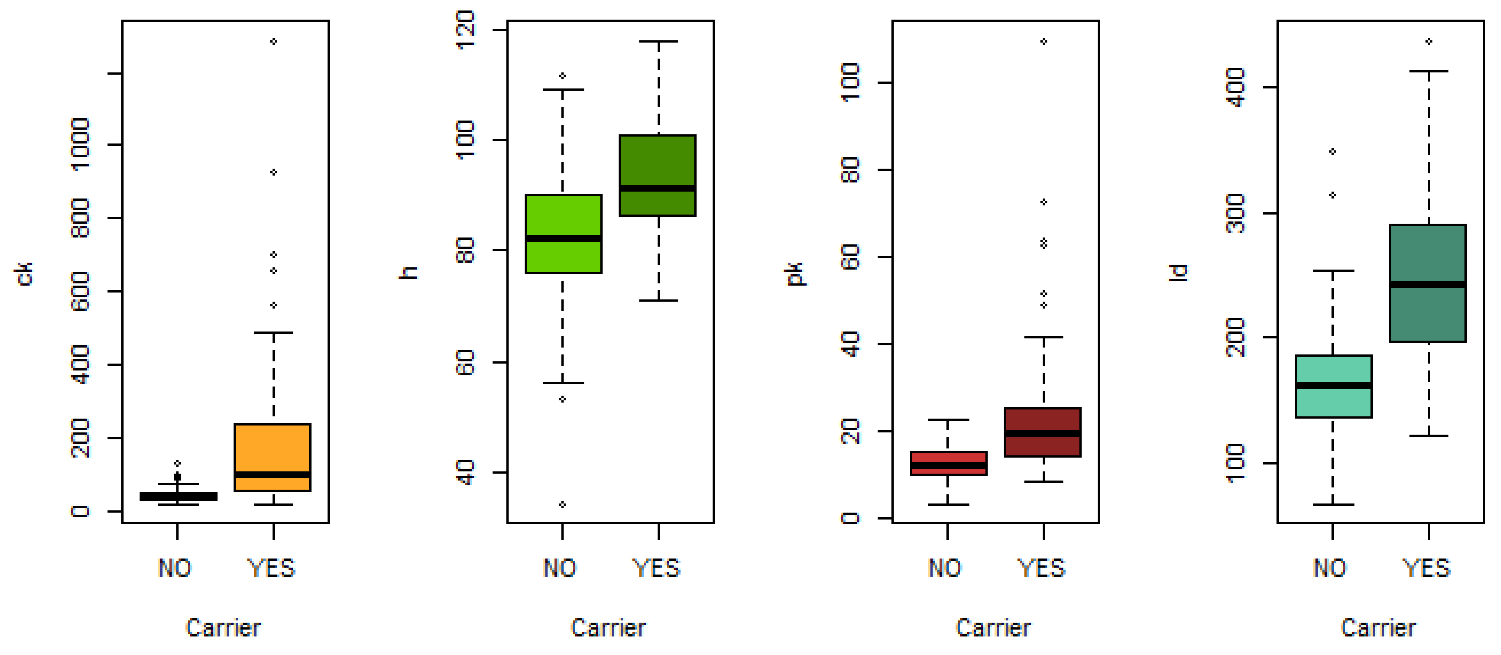
Duchenne muscular dystrophy (DMD) is a genetic disorder passed down from a mother to her children, causing progressive muscle weakness and wasting. Percy et al. [70] analysed the effectiveness of detecting this disorder using four biomarkers extracted from blood samples: serum creatine kinase (CK), haemopexin (H), pyruvate kinase (PK) and lactate dehydrogenase (LD). The dataset was obtained at https://hbiostat.org/data/, accessed on 30 January 2023. After removing observations with missing data, the dataset used contains information on the four biomarkers of 67 women who are carriers of the progressive recessive disorder DMD and 127 women who are not carriers.

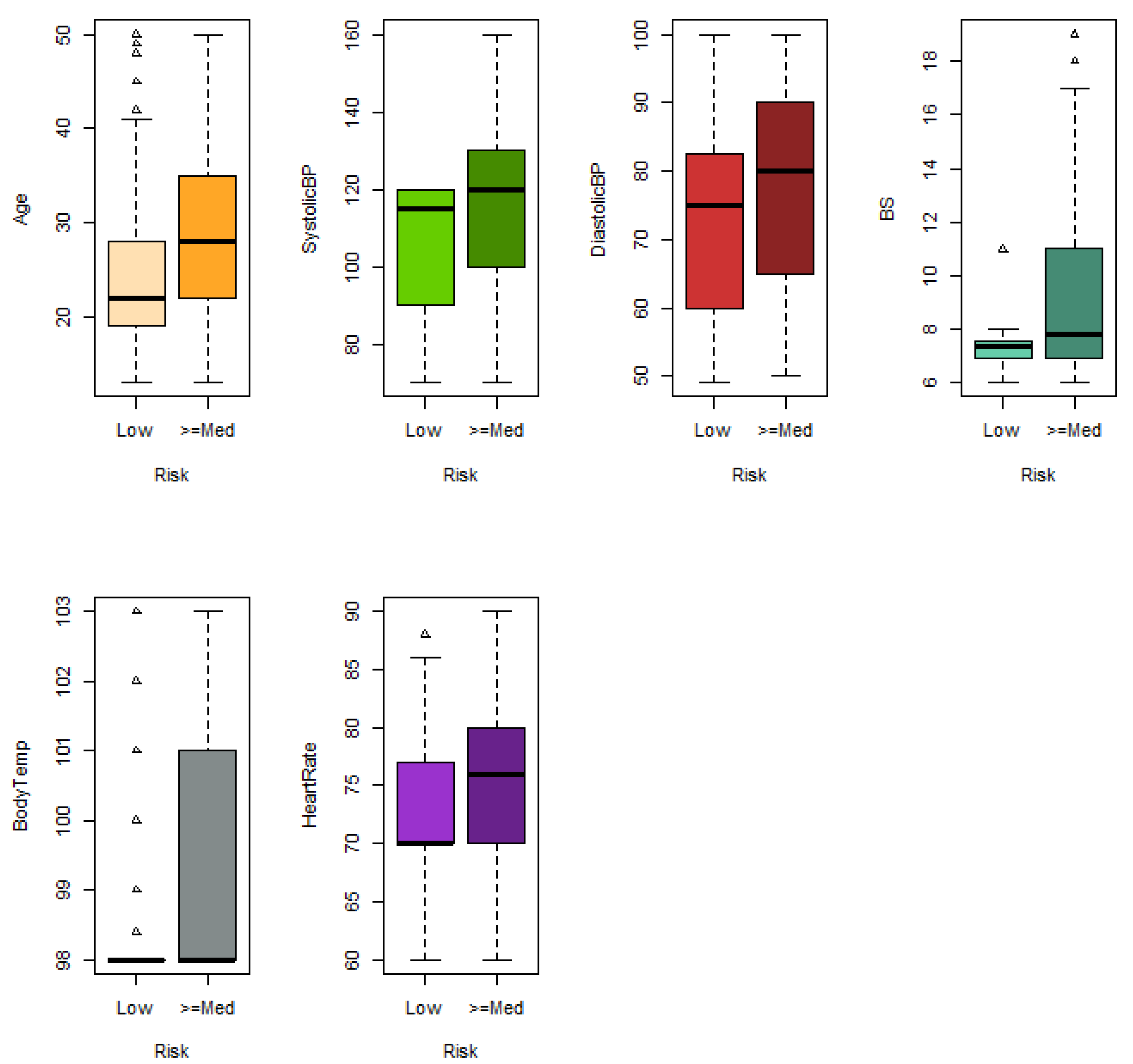
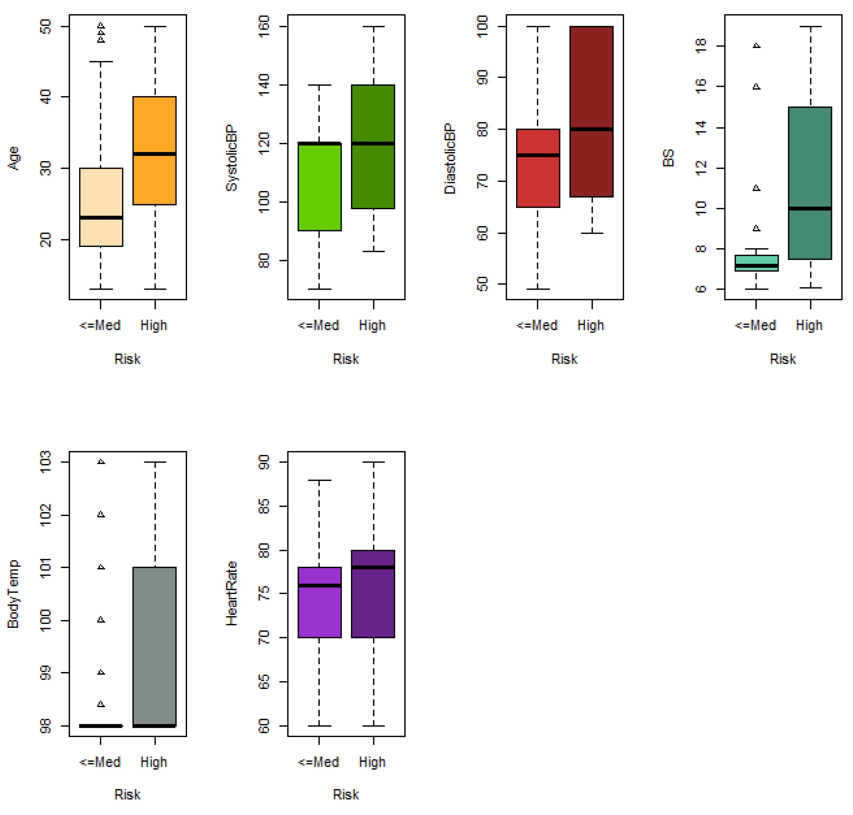
Maternal mortality refers to the death of a woman due to a pregnancy-related cause. It is one of the main concerns of the Sustainable Development Goals (SDG) of the United Nations. The dataset used for analysing maternal mortality was obtained at [71] (Maternal Health Risk), which contains information on the following six risk factors for maternal mortality: age in years during pregnant, upper value of blood pressure in mmHg (SystolicBP), lower value of blood pressure in mmHg (DiastolicBP), blood glucose levels in mmol/L (BS), body temperature in ºF (BodyTemp) and a normal resting heart rate in beats per minute (HeartRate). An IoT-based risk monitoring system was used to gather this information from various hospitals, community clinics, and maternal healthcare centres in the rural areas of Bangladesh. The level of risk intensity was also provided by differentiating three categories: low (406 women), medium (336 women) and high (272 women). To adapt data to our study, the following binary problems were considered: (i) predicting high or medium risk versus low risk and (ii) predicting high risk versus medium or low risk. The original dataset contains repeated data, outliers and anomalous data that may be due to errors in data retrieval. In our study, data from women aged 13–50 years were considered, duplicate rows were removed, and two observations were removed with heart rate values of 7 beats per minute, which is an erroneous value. Finally, the dataset used in the study contained 196 low-risk, 86 medium-risk and 95 high-risk observations.

2.8. Validation

A total of 59 simulated data scenarios were explored, considering different sample sizes, number of biomarkers, distributions, discriminatory ability, and correlations. For each simulated scenario, each method was trained considering random samples from the underlying distribution (100) and validated using new data simulated with the same configuration (100). For real data, a 10-fold cross-validation procedure was performed.

During training, the model parameters were estimated, and the optimal cut-off point that maximises the Youden index was obtained. The estimated model and the cut-off point selected were applied to the validation set. The Youden indices obtained in the validation set are shown in the tables in the following sections.

3. Results

This section presents the results of the performance achieved by each of the methods studied, both for the simulated scenarios and for the real data datasets. We denote the logistic regression, XGBoost, min–max approach, min–max–median approach, and min–max-IQR approach by LR, XG, MM, MMM, and MMIQR, respectively.

3.1. Simulations

The results obtained from the 100 random samples for each scenario are presented as the mean of the maximum Youden indices as well as the standard deviation. The following sections present the results for the symmetric (normal) and non-symmetric distribution scenarios.

3.1.1. Symmetric Distributions

Table 2. Normal distributions. Different means. Four biomarkers.

Size (${\mathit{n}}_1$,${\mathit{n}}_2$)	LR	XG	MM	MMM	MMIQR
Independents
(50,50)	0.453 (0.0919)	0.3878 (0.1016)	0.3696 (0.1037)	0.3884 (0.1075)	0.3938 (0.1107)
(500,500)	0.4882 (0.0282)	0.4698 (0.0322)	0.4103 (0.0308)	0.4397 (0.0317)	0.432 (0.0343)
High correlation (${\mathbf{\Sigma }}_{\mathbf{1}}={\mathbf{\Sigma }}_{\mathbf{2}}=\mathbf{0.3}·\mathit{I}+\mathbf{0.7}·\mathit{J}$)
(50,50)	0.4392 (0.0904)	0.3598 (0.1004)	0.2652 (0.106)	0.249 (0.0925)	0.2646 (0.0892)
(500,500)	0.4653 (0.0286)	0.4457 (0.0315)	0.2966 (0.0367)	0.2954 (0.0378)	0.2963 (0.0362)
Different Correlation (${\mathbf{\Sigma }}_{\mathbf{1}}=\mathbf{0.3}·\mathit{I}+\mathbf{0.7}·\mathit{J}$, ${\mathbf{\Sigma }}_{\mathbf{2}}=\mathbf{0.7}·\mathit{I}+\mathbf{0.3}·\mathit{J}$)
(50,50)	0.392 (0.0933)	0.3758 (0.0946)	0.3212 (0.0978)	0.3288 (0.0892)	0.3194 (0.1007)
(500,500)	0.4262 (0.031)	0.4814 (0.0314)	0.3564 (0.0323)	0.3593 (0.0306)	0.3598 (0.0307)
Negative Correlation ($\rho =-0.1$)
(50,50)	0.5074 (0.0808)	0.4578 (0.0857)	0.4358 (0.0826)	0.4708 (0.0802)	0.461 (0.0841)
(500,500)	0.5562 (0.0239)	0.5306 (0.0245)	0.4658 (0.027)	0.5147 (0.0279)	0.5053 (0.0323)

and

Table 3. Normal distributions. Same means. Four biomarkers.

Size (${\mathit{n}}_1$,${\mathit{n}}_2$)	LR	XG	MM	MMM	MMIQR
Low correlation (${\mathbf{\Sigma }}_{\mathbf{1}}={\mathbf{\Sigma }}_{\mathbf{2}}=\mathbf{0.7}·\mathit{I}+\mathbf{0.3}·\mathit{J}$)
(50,50)	0.4878 (0.09)	0.429 (0.0942)	0.4794 (0.0954)	0.482 (0.097)	0.4818 (0.0971)
(500,500)	0.5254 (0.0285)	0.5125 (0.0284)	0.5073 (0.0278)	0.5183 (0.032)	0.5182 (0.0295)
Different Correlation (${\mathbf{\Sigma }}_{\mathbf{1}}=\mathbf{0.3}·\mathit{I}+\mathbf{0.7}·\mathit{J}$, ${\mathbf{\Sigma }}_{\mathbf{2}}=\mathbf{0.7}·\mathit{I}+\mathbf{0.3}·\mathit{J}$)
(50,50)	0.4598 (0.0958)	0.4628 (0.1004)	0.5366 (0.0904)	0.5438 (0.0813)	0.5398 (0.0869)
(500,500)	0.4783 (0.0259)	0.5279 (0.0284)	0.5609 (0.0285)	0.5627 (0.0271)	0.5632 (0.0271)
Different Correlation (${\mathbf{\Sigma }}_{\mathbf{1}}=\mathbf{0.5}·\mathit{I}+\mathbf{0.5}·\mathit{J}$, ${\mathbf{\Sigma }}_{\mathbf{2}}=\mathit{I}$)
(50,50)	0.5452 (0.0779)	0.5186 (0.0831)	0.5758 (0.0776)	0.587 (0.0825)	0.59 (0.0771)
(500,500)	0.5748 (0.028)	0.5875 (0.0289)	0.5975 (0.0279)	0.6097 (0.0247)	0.6088 (0.0246)

display the results obtained from the simulated scenarios for $p=4$ biomarkers following a multivariate normal distribution with different means and the same means, respectively. The code can be found at Supplementary Material: Chapter 1, Sections A.1.–A.5.

The results in Table 2 show, in general, a superiority of logistic regression over the other algorithms, except in the scenario of different correlations and larger sample sizes, where XGBoost significantly outperforms it. Our proposed algorithms (MMM/MMIQR) show similar performance to the min–max approach or superior, particularly when biomarkers are independent or negatively correlated.

Table 3 presents the results for biomarkers with the same predictive ability. The conclusions derived are different from those in the Table 2 above (different mean). Logistic regression achieves the highest average performance value in the same and low correlation scenarios, although the rest of the algorithms obtained very close values. The summary-statistics-based methods (MM, MMM, MMIQR) and especially our proposed algorithms (MMM/MMIQR) outperformed the other algorithms in scenarios with different correlations. XGBoost outperforms logistic regression in scenarios with different correlations and large sample sizes.

Table 4. Normal distributions. Different means. Ten biomarkers.

Size (${\mathit{n}}_1$,${\mathit{n}}_2$)	LR	XG	MM	MMM	MMIQR
Independents
(50,50)	0.8698 (0.055)	0.86 (0.061)	0.7704 (0.0642)	0.8716 (0.0547)	0.8616 (0.0647)
(500,500)	0.9448 (0.0093)	0.9288 (0.0142)	0.7962 (0.0187)	0.8996 (0.0146)	0.8993 (0.0175)
High correlation (${\mathbf{\Sigma }}_{\mathbf{1}}={\mathbf{\Sigma }}_{\mathbf{2}}=\mathbf{0.3}·\mathit{I}+\mathbf{0.7}·\mathit{J}$)
(50,50)	0.8324 (0.0696)	0.7992 (0.0726)	0.6672 (0.0854)	0.6644 (0.0868)	0.662 (0.0861)
(500,500)	0.9191 (0.0149)	0.8935 (0.0168)	0.6893 (0.0245)	0.6899 (0.0253)	0.6888 (0.0271)
Different Correlation (${\mathbf{\Sigma }}_{\mathbf{1}}=\mathbf{0.3}·\mathit{I}+\mathbf{0.7}·\mathit{J}$, ${\mathbf{\Sigma }}_{\mathbf{2}}=\mathbf{0.7}·\mathit{I}+\mathbf{0.3}·\mathit{J}$)
(50,50)	0.789 (0.071)	0.7658 (0.0706)	0.4924 (0.0932)	0.4948 (0.0961)	0.4982 (0.0977)
(500,500)	0.8585 (0.0174)	0.8626 (0.0179)	0.5287 (0.0274)	0.5471 (0.0255)	0.5464 (0.0248)
Negative Correlation ($\rho =-0.1$)
(50,50)	0.9232 (0.0552)	0.8884 (0.075)	0.865 (0.0599)	0.9468 (0.0482)	0.9576 (0.0418)
(500,500)	0.9936 (0.0042)	0.9764 (0.0145)	0.8953 (0.0166)	0.996 (0.0035)	0.9962 (0.0034)

and

Table 5. Normal distributions. Same means. Ten biomarkers..

Size (${\mathit{n}}_1$,${\mathit{n}}_2$)	LR	XG	MM	MMM	MMIQR
Low correlation (${\mathbf{\Sigma }}_{\mathbf{1}}={\mathbf{\Sigma }}_{\mathbf{2}}=\mathbf{0.7}·\mathit{I}+\mathbf{0.3}·\mathit{J}$)
(50,50)	0.5216 (0.09)	0.508 (0.0833)	0.5202 (0.0812)	0.5328 (0.0885)	0.531 (0.0841)
(500,500)	0.5803 (0.0264)	0.5595 (0.0255)	0.5501 (0.0281)	0.5742 (0.0302)	0.5751 (0.0285)
Different Correlation (${\mathbf{\Sigma }}_{\mathbf{1}}=\mathbf{0.3}·\mathit{I}+\mathbf{0.7}·\mathit{J}$, ${\mathbf{\Sigma }}_{\mathbf{2}}=\mathbf{0.7}·\mathit{I}+\mathbf{0.3}·\mathit{J}$)
(50,50)	0.4206 (0.1047)	0.4662 (0.106)	0.6784 (0.0758)	0.6774 (0.0821)	0.6766 (0.08)
(500,500)	0.5044 (0.0283)	0.6324 (0.0279)	0.692 (0.0226)	0.6929 (0.0233)	0.6946 (0.0242)
Different Correlation (${\mathbf{\Sigma }}_{\mathbf{1}}=\mathbf{0.5}·\mathit{I}+\mathbf{0.5}·\mathit{J}$, ${\mathbf{\Sigma }}_{\mathbf{2}}=\mathit{I}$)
(50,50)	0.621 (0.0816)	0.6146 (0.0819)	0.6966 (0.0751)	0.7172 (0.0706)	0.718 (0.0715)
(500,500)	0.6849 (0.0237)	0.714 (0.0257)	0.712 (0.0203)	0.7373 (0.025)	0.7378 (0.0253)

present the results obtained considering the above scenarios for $p=10$ biomarkers. The code can be found at Supplementary Material: Chapter 1, Sections A.6.–A.10. Table 4 shows the Youden indices achieved for biomarkers with different means. The conclusions derived are similar to those in Table 2, with our more hardened approaches being significantly superior to the min–max approach, especially when biomarkers are independent or negatively correlated, where they achieve the best performance. Logistic regression generally outperforms all other algorithms in all other scenarios.

The results reported in Table 5 show similar behaviour to Table 3. In general, the summary statistics-based methods and, in particular, our approaches outperform the others. The XGBoost algorithm outperforms logistic regression, generally, in the different correlation scenarios.

3.1.2. Asymmetric Distributions

This section presents results derived from simulated scenarios of non-normal distributions.

Table 6. Log-normal distributions. Different means. Four biomarkers.

Size (${\mathit{n}}_1$,${\mathit{n}}_2$)	LR	XG	MM	MMM	MMIQR
Independents
(50,50)	0.4112 (0.0936)	0.385 (0.1016)	0.3658 (0.106)	0.393 (0.1031)	0.3852 (0.1077)
(500,500)	0.4562 (0.03)	0.4686 (0.0313)	0.4096 (0.0324)	0.4376 (0.0315)	0.435 (0.0328)
High correlation (${\mathbf{\Sigma }}_{\mathbf{1}}={\mathbf{\Sigma }}_{\mathbf{2}}=\mathbf{0.3}·\mathit{I}+\mathbf{0.7}·\mathit{J}$)
(50,50)	0.4108 (0.1009)	0.354 (0.0998)	0.2596 (0.1025)	0.2468 (0.1004)	0.246 (0.102)
(500,500)	0.4502 (0.0282)	0.446 (0.0318)	0.2954 (0.0365)	0.2935 (0.037)	0.2935 (0.0337)
Different Correlation (${\mathbf{\Sigma }}_{\mathbf{1}}=\mathbf{0.3}·\mathit{I}+\mathbf{0.7}·\mathit{J}$, ${\mathbf{\Sigma }}_{\mathbf{2}}=\mathbf{0.7}·\mathit{I}+\mathbf{0.3}·\mathit{J}$)
(50,50)	0.3492 (0.0955)	0.3814 (0.0879)	0.3158 (0.0942)	0.3198 (0.0955)	0.3166 (0.102)
(500,500)	0.394 (0.0337)	0.4815 (0.0328)	0.3558 (0.0325)	0.3571 (0.0317)	0.3567 (0.0334)
Negative Correlation ($\rho =-0.1$)
(50,50)	0.4538 (0.0963)	0.4466 (0.0861)	0.4268 (0.0834)	0.4794 (0.0795)	0.4802 (0.0853)
(500,500)	0.4916 (0.0264)	0.5304 (0.0252)	0.4627 (0.0248)	0.5051 (0.0274)	0.5044 (0.0278)

,

Table 7. Log-normal distributions. Same means. Four biomarkers.

Size (${\mathit{n}}_1$,${\mathit{n}}_2$)	LR	XG	MM	MMM	MMIQR
Low correlation (${\mathbf{\Sigma }}_{\mathbf{1}}={\mathbf{\Sigma }}_{\mathbf{2}}=\mathbf{0.7}·\mathit{I}+\mathbf{0.3}·\mathit{J}$)
(50,50)	0.4592 (0.0955)	0.4312 (0.0943)	0.4704 (0.0933)	0.483 (0.0879)	0.4816 (0.095)
(500,500)	0.5049 (0.0301)	0.5121 (0.029)	0.5051 (0.027)	0.5161 (0.0282)	0.5151 (0.0282)
Different Correlation (${\mathbf{\Sigma }}_{\mathbf{1}}=\mathbf{0.3}·\mathit{I}+\mathbf{0.7}·\mathit{J}$, ${\mathbf{\Sigma }}_{\mathbf{2}}=\mathbf{0.7}·\mathit{I}+\mathbf{0.3}·\mathit{J}$)
(50,50)	0.4066 (0.0926)	0.4524 (0.1019)	0.5444 (0.0911)	0.5358 (0.0905)	0.54 (0.0884)
(500,500)	0.4166 (0.0279)	0.5292 (0.0278)	0.5606 (0.0266)	0.5607 (0.0276)	0.56 (0.0279)
Different Correlation (${\mathbf{\Sigma }}_{\mathbf{1}}=\mathbf{0.5}·\mathit{I}+\mathbf{0.5}·\mathit{J}$, ${\mathbf{\Sigma }}_{\mathbf{2}}=\mathit{I}$)
(50,50)	0.4556 (0.0853)	0.522 (0.0755)	0.5784 (0.0813)	0.5832 (0.0865)	0.5798 (0.0897)
(500,500)	0.4755 (0.0282)	0.5881 (0.0288)	0.5982 (0.0276)	0.6074 (0.025)	0.6079 (0.0258)

and

Table 8. Different marginal distributions.Four biomarkers.

Size (${\mathit{n}}_1$,${\mathit{n}}_2$)	LR	XG	MM	MMM	MMIQR
(50,50)	0.6572 (0.108)	0.6838 (0.0947)	0.3716 (0.1194)	0.3442 (0.1234)	0.3616 (0.1251)
(500,500)	0.7065 (0.0363)	0.7692 (0.0220)	0.435 (0.0453)	0.4357 (0.0442)	0.4358 (0.0429)

show the results obtained from simulated data for $p=4$ biomarkers. The code can be found in Supplementary Material: Chapter 1, Sections B.1.–B.6. Specifically, Table 6 and Table 7 consider scenarios under log-normal distribution and Table 8 considering different marginal distributions (${\chi }^2$, normal, gamma and exponential).

Table 9. Log-normal distributions. Different means. Ten biomarkers.

Size (${\mathit{n}}_1$,${\mathit{n}}_2$)	LR	XG	MM	MMM	MMIQR
Independents
(50,50)	0.8344 (0.0556)	0.8594 (0.065)	0.7728 (0.0632)	0.8772 (0.0545)	0.8646 (0.0591)
(500,500)	0.901 (0.0137)	0.9293 (0.0128)	0.7966 (0.018)	0.895 (0.0154)	0.8929 (0.0178)
High correlation (${\mathbf{\Sigma }}_{\mathbf{1}}={\mathbf{\Sigma }}_{\mathbf{2}}=\mathbf{0.3}·\mathit{I}+\mathbf{0.7}·\mathit{J}$)
(50,50)	0.817 (0.0706)	0.8034 (0.0745)	0.6584 (0.0762)	0.6572 (0.0828)	0.657 (0.0805)
(500,500)	0.8948 (0.0164)	0.8916 (0.0173)	0.6825 (0.0224)	0.6812 (0.0244)	0.6814 (0.0248)
Different Correlation (${\mathbf{\Sigma }}_{\mathbf{1}}=\mathbf{0.3}·\mathit{I}+\mathbf{0.7}·\mathit{J}$, ${\mathbf{\Sigma }}_{\mathbf{2}}=\mathbf{0.7}·\mathit{I}+\mathbf{0.3}·\mathit{J}$)
(50,50)	0.7436 (0.0795)	0.7692 (0.077)	0.4994 (0.0932)	0.505 (0.0961)	0.5026 (0.097)
(500,500)	0.808 (0.0217)	0.8626 (0.018)	0.5218 (0.0279)	0.5452 (0.0257)	0.5445 (0.025)
Negative Correlation ($\rho =-0.1$)
(50,50)	0.8946 (0.0586)	0.886 (0.0755)	0.8704 (0.05)	0.952 (0.0449)	0.953 (0.0457)
(500,500)	0.9703 (0.01)	0.9756 (0.0143)	0.8938 (0.0149)	0.9947 (0.0044)	0.9964 (0.0036)

and

Table 10. Log-normal distributions. Same means.Ten biomarkers.

Size (${\mathit{n}}_1$,${\mathit{n}}_2$)	LR	XG	MM	MMM	MMIQR
Low correlation (${\mathbf{\Sigma }}_{\mathbf{1}}={\mathbf{\Sigma }}_{\mathbf{2}}=\mathbf{0.7}·\mathit{I}+\mathbf{0.3}·\mathit{J}$)
(50,50)	0.5072 (0.0917)	0.5066 (0.0859)	0.5144 (0.0869)	0.5306 (0.0931)	0.5344 (0.0886)
(500,500)	0.5656 (0.0253)	0.5592 (0.0292)	0.5459 (0.0277)	0.5739 (0.0296)	0.5748 (0.0288)
Different Correlation (${\mathbf{\Sigma }}_{\mathbf{1}}=\mathbf{0.3}·\mathit{I}+\mathbf{0.7}·\mathit{J}$, ${\mathbf{\Sigma }}_{\mathbf{2}}=\mathbf{0.7}·\mathit{I}+\mathbf{0.3}·\mathit{J}$)
(50,50)	0.35 (0.1058)	0.4666 (0.1037)	0.6732 (0.0852)	0.661 (0.091)	0.664 (0.0905)
(500,500)	0.4253 (0.0277)	0.6321 (0.0275)	0.6796 (0.0239)	0.6802 (0.0254)	0.6811 (0.0251)
Different Correlation (${\mathbf{\Sigma }}_{\mathbf{1}}=\mathbf{0.5}·\mathit{I}+\mathbf{0.5}·\mathit{J}$, ${\mathbf{\Sigma }}_{\mathbf{2}}=\mathit{I}$)
(50,50)	0.4944 (0.0835)	0.613 (0.0756)	0.69 (0.0789)	0.7166 (0.0762)	0.7186 (0.0782)
(500,500)	0.5506 (0.0265)	0.715 (0.0239)	0.7122 (0.0225)	0.738 (0.0231)	0.7376 (0.0222)

display the results obtained from simulated data for $p=10$ biomarkers following a log-normal distribution. The code can be found in Supplementary Material: Chapter 1, Sections B.7.–B.11.

Table 6 reports results for the scenario of biomarkers with different means. It shows tnat logistic regression outperforms the others in high-correlation scenarios. The XGBoost algorithm dominates the others in all other scenarios for larger sample sizes and in all scenarios of different correlations. Our min–max-IQR approach outperforms the others in small sample sizes of negative correlations and particularly the min–max approach in the independent biomarker scenarios.

The results reported in Table 7 show a similar behaviour to Table 3 (normal distributions) but with a worse logistic regression performance, such that our approaches generally perform the best in all scenarios.

The results in Table 8 indicate that, in scenarios of different marginal distributions, the XGBoost algorithm dominates the rest significantly. In these scenarios, the summary statistics-based methods are the worst performers.

Table 9 shows that logistic regression outperforms the rest in high-correlation scenarios but is closely followed by the XGBoost algorithm. The XGBoost algorithm dominates over the others in independent scenarios of larger sample sizes and scenarios with different correlations between groups. Our approaches achieve the best performance in independent biomarker scenarios and smaller sample sizes and in scenarios with negative correlations.

The results reported in Table 10 show a general dominance of our approaches over the others, with logistic regression performing significantly worse in scenarios of different correlation than in other scenarios.

3.1.3. Summary

To provide a better understanding of our proposed approaches’ performance compared to other algorithms, this section provides a summary of the previously displayed results in Figure 1 and Figure 2. Figure 1 shows the results from simulated scenarios of normal distributions, while Figure 2 displays the results from non-normal distributions. The value on the y-axis represents the value after subtracting the average Youden index achieved by our proposed best approach (MMM or MMMIQR) among the other algorithms: logistic regression, XGBoost and min–max approach. The blue value corresponds to the difference with logistic regression (denoted by MMM-LR), red with XGBoost algorithm (MMM-XG), and black with min–max approach (MMM-MM). Thus, negative values on the graph represent scenarios where algorithms outperform our approaches and positive values in other scenarios. The further away from zero, the more significant the difference.

Regarding scenarios with normal distributions (Figure 1), machine learning algorithms (logistic regression and XGBoost algorithm) outperform our approaches, particularly in scenarios with biomarkers with different predictive capacity, mainly in scenarios with high correlations and different correlations (scenarios 2 and 3). However, our approaches outperform the others in scenarios with biomarkers with similar predictive ability (scenarios 5–7) and in scenarios of biomarkers with negative correlations, mainly for scenarios with a higher number of biomarkers. Note that these differences are more pronounced in scenarios with a higher number of biomarkers.

As for the scenarios of non-normal distributions (Figure 2), the behaviour in scenarios of log-normal distributions is similar to those with normal distributions (Figure 1 above), but with larger differences overall in favour of our algorithm with respect to logistic regression in scenarios with biomarkers of the same means. In scenarios where biomarkers follow different marginal distributions, the XGBoost algorithm significantly achieves the best performance. XGBoost also outperforms the others in scenarios of biomarkers with different means and different variance-covariance matrices between groups.

3.2. Real Datasets

3.2.1. Duchenne Muscular Dystrophy

Figure 3 shows the distribution of each biomarker, and

Table 11. Correlation between biomarkers. DMD dataset.

	${\mathit{r}}_{\mathit{CK}-\mathit{H}}$	${\mathit{r}}_{\mathit{CK}-\mathit{PK}}$	${\mathit{r}}_{\mathit{CK}-\mathit{LD}}$	${\mathit{r}}_{\mathit{H}-\mathit{PK}}$	${\mathit{r}}_{\mathit{H}-\mathit{LD}}$	${\mathit{r}}_{\mathit{PK}-\mathit{LD}}$
Non-Carrier	−0.33	0.1	0.2	0.08	0.18	0.22
Carrier	−0.14	0.7	0.49	−0.12	−0.1	0.48

displays the correlation matrix between them in each group (67 carriers and 127 non-carriers) for the Duchenne muscular dystrophy dataset, where $r_{CK-H}$ denotes the correlation between the pair of biomarkers CK and H. The code can be found in Supplementary Material: Chapter 2, Section A.1.

Because the range of biomarker values differs from the others, the values of each biomarker were normalised before applying summary statistics-based methods, thus ensuring the correct use of these methods. The biomarkers CK and H show a negative correlation, which is stronger in the non-carrier group. Conversely, the other biomarker pairs generally show positive correlations, with a stronger correlation observed in the carrier group.

The estimates of the Youden index of each biomarker (CK, H, PK, LD) produced in a univariate way on the whole dataset were 0.612, 0.417, 0.508, and 0.578.

Table 12. Ten-fold cross-validation. DMD dataset.

Algorithm	Youden	Sensitivity	Specificity
LR	0.8008	0.8476	0.9532
XG	0.7047	0.8142	0.8905
MM	0.6258	0.7952	0.8306
MMM	0.7793	0.8595	0.9198
MMIQR	0.7772	0.8761	0.9011

presents the average value of the maximum Youden indices achieved in each fold for each of the analysed methods, as well as their respective values of sensitivity and specificity. The code can be found in Supplementary Material: Chapter 2, Section A.2.

Logistic regression achieved the best performance, although our approaches are not far behind, outperforming the XGBoost algorithm and notably the min–max approach.

3.2.2. Maternal Health Risk

This section presents the performance results of the approaches to the problem of predicting high or medium versus low risk of maternal mortality (High–Medium vs. Low Risk) and the problem of predicting high risk versus low or medium risk of maternal mortality (High vs. Medium–Low Risk) for the Maternal Health Risk dataset.

3.2.3. High–Medium vs. Low Risk

Figure 4 displays the distribution of each variable, and

Table 13. Correlation between biomarkers. Maternal Health dataset. High–Medium vs. Low Risk.

	${\mathit{r}}_{\mathit{V}1-\mathit{V}2}$	${\mathit{r}}_{\mathit{V}1-\mathit{V}3}$	${\mathit{r}}_{\mathit{V}1-\mathit{V}4}$	${\mathit{r}}_{\mathit{V}1-\mathit{V}5}$	${\mathit{r}}_{\mathit{V}1-\mathit{V}6}$	${\mathit{r}}_{\mathit{V}2-\mathit{V}3}$	${\mathit{r}}_{\mathit{V}2-\mathit{V}4}$	${\mathit{r}}_{\mathit{V}2-\mathit{V}5}$	${\mathit{r}}_{\mathit{V}2-\mathit{V}6}$	${\mathit{r}}_{\mathit{V}3-\mathit{V}4}$	${\mathit{r}}_{\mathit{V}3-\mathit{V}5}$	${\mathit{r}}_{\mathit{V}3-\mathit{V}6}$	${\mathit{r}}_{\mathit{V}4-\mathit{V}5}$	${\mathit{r}}_{\mathit{V}4-\mathit{V}5}$	${\mathit{r}}_{\mathit{V}5-\mathit{V}6}$
Low Risk	0.39	0.4	0.17	−0.13	−0.17	0.8	0.07	−0.08	−0.15	0.11	−0.1	−0.09	0.03	−0.02	0.11
High–Medium Risk	0.46	0.39	0.53	−0.38	0.08	0.75	0.27	−0.41	−0.07	0.27	−0.36	−0.14	−0.17	0.19	0.12

shows the correlation matrix between them in each group (196 low risk and 181 medium-high risk). The variables Age, SystolicBP, DiastolicBP, BS, BodyTemp and HeartRate are denoted by V1, V2, V3, V4, V5, and V6, respectively. The code can be found in Supplementary Material: Chapter 2, Section B.1.

Positive and negative correlations are shown between the variables, generally with greater strength in the higher-risk group (High–Medium Risk). The estimates of the Youden index of each biomarker (Age, SystolicBP, DiastolicBP, BS, BodyTemp and HeartRate) produced in a univariate way on the whole dataset were 0.305, 0.304, 0.153, 0.377, 0.249, 0.217, respectively. The predictive capacity of the biomarkers in this dataset was lower than the previously presented DMD dataset, as can also be seen in Figure 4.

Table 14. Ten-fold cross-validation. Maternal Health dataset. High–Medium vs.Low Risk.

Algorithm	Youden	Sensitivity	Specificity
LR	0.5366	0.6611	0.8755
XG	0.586	0.74	0.846
MM	0.4563	0.7055	0.7508
MMM	0.4739	0.718	0.7559
MMIQR	0.4739	0.718	0.7559

presents the performance achieved by each of the analysed methods after the application of 10-fold cross-validation. The values of each biomarker were normalised before applying the summary statistics-based methods. The code can be found in Supplementary Material: Chapter 2, Section B.2.

The XGBoost algorithm and logistic regression achieved better performance than the summary-statistics-based methods, especially XGBoost which performs the best.

3.2.4. High vs. Medium–Low Risk

Figure 5 shows the distribution of each variable and

Table 15. Correlation between biomarkers. Maternal Health dataset. High vs. Medium–Low Risk.

	${\mathit{r}}_{\mathit{V}1-\mathit{V}2}$	${\mathit{r}}_{\mathit{V}1-\mathit{V}3}$	${\mathit{r}}_{\mathit{V}1-\mathit{V}4}$	${\mathit{r}}_{\mathit{V}1-\mathit{V}5}$	${\mathit{r}}_{\mathit{V}1-\mathit{V}6}$	${\mathit{r}}_{\mathit{V}2-\mathit{V}3}$	${\mathit{r}}_{\mathit{V}2-\mathit{V}4}$	${\mathit{r}}_{\mathit{V}2-\mathit{V}5}$	${\mathit{r}}_{\mathit{V}2-\mathit{V}6}$	${\mathit{r}}_{\mathit{V}3-\mathit{V}4}$	${\mathit{r}}_{\mathit{V}3-\mathit{V}5}$	${\mathit{r}}_{\mathit{V}3-\mathit{V}6}$	${\mathit{r}}_{\mathit{V}4-\mathit{V}5}$	${\mathit{r}}_{\mathit{V}4-\mathit{V}5}$	${\mathit{r}}_{\mathit{V}5-\mathit{V}6}$
Medium–Low Risk	0.44	0.41	0.33	−0.14	−0.13	0.74	0.18	−0.08	−0.16	0.17	−0.1	−0.16	0.05	0.03	0.22
High Risk	0.44	0.4	0.55	−0.57	0.06	0.84	0.23	−0.57	−0.04	0.18	−0.54	−0.09	−0.4	0.14	−0.01

the correlation matrix between them in each group (282 low–medium risk and 95 high risk). Age, SystolicBP, DiastolicBP, BS, BodyTemp and HeartRate are denoted by V1, V2, V3, V4, V5 and V6, respectively. The code can be found in Supplementary Material: Chapter 2, Section C.1.

As in the previous example, positive and negative correlations between pairs of variables are shown. The Youden index estimates for each biomarker (Age, SystolicBP, DiastolicBP, BS, BodyTemp and HeartRate) univariate over the whole dataset were 0.347, 0.386, 0.268, 0.564, 0.22 and 0.272, respectively, which are higher than in the previous example.

Table 16. Ten-fold cross-validation. Maternal Health dataset. High vs. Medium–Low Risk.

Algorithm	Youden	Sensitivity	Specificity
LR	0.6225	0.8036	0.849
XG	0.7159	0.8238	0.8921
MM	0.6149	0.8932	0.7217
MMM	0.5831	0.8851	0.6981
MMIQR	0.5831	0.8851	0.6981

displays the performance achieved for each of the analysed methods. The values of each biomarker were normalised before applying the summary statistics-based methods. The code can be found in Supplementary Material: Chapter 2, Section C.2.

The XGBoost algorithm significantly outperformed the other algorithms. It was followed by logistic regression, but the summary-statistics-based algorithm was not far behind.

4. Discussion and Conclusions

In binary classification problems in healthcare, the choice of thresholds to dichotomise the model output into groups of patients is crucial and can aid decision-making in clinical practice. In the absence of consensus on the benefits of optimising the classification of one group or another, the Youden index is a standard criterion that provides good performance for the model.

Models combining biomarkers for binary classification have received sufficient attention in the literature. The parametric approach has the limitation of meeting the assumption of normality; by contrast, other authors propose non-parametric approaches without assumptions of biomarker distributions but with the limitation of being computationally intractable when the number of biomarkers increases.

Liu et al. [19] proposed the min–max approach, which is a non-parametric and computationally tractable approach regardless of the number of biomarkers, based on the linear combination of minimum and maximum values of biomarkers. The idea behind this proposal is that the maximum and minimum values chosen among the biomarkers can allow the best discrimination between sick and healthy patients. However, this approach may not be sufficient in terms of discrimination when the number of biomarkers grows, because it is not enough to capture all the discrimination abilities of the set of predictor variables. To improve the min–max algorithm, we proposed the min–max–median/IQR approach under a Youden index maximisation that incorporates a new summary statistic with reasonably good performance. This approach uses a stepwise algorithm that we proposed in [25], which is based on the work of Pepe et al. [14,15].

The use of machine learning algorithms, such as XGBoost, has become increasingly popular in recent years due to their ease of implementation and good results. However, the choice of the optimal approach depends on the problem and the data to be processed. It is therefore essential to make a thorough comparison before providing some guidelines for the selection of the optimal algorithm.

The aim of this paper is to present a comprehensive comparison of our min–max–median/IQR approaches with the min–max approach and machine learning algorithms such as logistic regression and XGBoost, in order to optimise the Youden index. For this purpose, the algorithms were compared on 59 different simulated data scenarios with symmetric and non-symmetric distributions, as well as on two real-world datasets.

The results of the simulated scenarios showed that the machine learning approaches outperformed our approaches, in particular in scenarios with biomarkers with different predictive abilities and in biomarker scenarios with different marginal distributions. However, our approaches outperformed them in scenarios with biomarkers with normal and log-normal distributions with the same predictive ability and different correlations between groups.

Regarding the real datasets, XGBoost outperformed the other algorithms in predicting maternal health risk, while logistic regression achieved the best performance in predicting Duchenne dystrophy, with our proposed approaches closely following. The data show that the problem of predicting Duchenne dystrophy is simpler than that of predicting maternal death risk. In the former, linear combination approaches outperform XGBoost. However, XGBoost outperforms the others on the more complex problem. This may be due to its ability to capture non-linear relationships.

In summary, regardless of the symmetry assumption, non-parametric approaches are always a good alternative for modelling data, but their performance is not guaranteed. Therefore, the modelling process requires a combination of techniques and the optimization of hyperparameters, as we have demonstrated with extensive simulations and application on real data. This work provides the scientific community with a comparison of the performance of our approaches (min–max–median/IQR) and machine learning algorithms, that can be applied and explored in different binary classification problems, such as cancer diagnosis. We proposed a non-parametric approach, addressing the limitations of previous linear biomarker combinations that assume multivariate normality. It also addresses the limitation of the computational burden of certain approaches in the literature, being always approachable regardless of the number of initial biomarkers. This is achieved thanks to the formulation of our algorithm that linearly combines the minimum, maximum, and median or interquartile range biomarkers, thereby converting the n-biomarker combination problem into a three-biomarker combination problem. Although there are several techniques that reduce the dimensionality of the problem for subsequent classification algorithm application, our proposed approach provides a different perspective in this regard. The way our approach is formulated allows the three biomarkers considered (minimum, maximum and median or interquartile range) to correspond to different original biomarkers for each patient. This offers the possibility of capturing biomarker heterogeneity in the data. Subsequently, our approach applies a stepwise algorithm, which we published in [25] , and which demonstrated acceptable performance in the comparison study. Therefore, our approach proposes a novel formulation in the state of the art that addresses certain limitations in the literature. Furthermore, a comparison of our approach with other approaches, such as the XGBoost algorithm, provides performance results with other approaches that also help to capture biomarker heterogeneity, albeit from a different perspective. XGBoost is a decision tree ensemble algorithm that builds multiple trees and combines their predictions to produce the final output. For the construction of each tree, a random subset of biomarkers/variables is selected and used to partition the data. In this way, each tree is constructed with information from different biomarkers, thus helping to avoid overfitting.

Our approaches have been shown to be superior to other algorithms, including machine learning algorithms, in scenarios with biomarkers having the same predictive capacity and different correlations between groups. These results are not surprising, as there is a variety of health problems in which the combination of the minimum and maximum of biomarkers provides the best classification. In prostate cancer, the worst diagnosis corresponds to a higher value in PSA and a lower value in prostate volume. PSA density is defined by the division of PSA and prostate volume, and it shows a better predictive ability than PSA. Thus, we can choose as a biomarker for prostate cancer the PSA density or the combination provided by PSA and prostate volume. Moreover, as with PSA, there is a variety of competing biomarkers such as PCA3, SelectMdx, and 4Kscore, in which high values correspond to a greater probability of cancer. The min–max derived approaches gives the opportunity to choose from them the one which takes the highest value. Similar to prostate volume, the free PSA takes lower values with a worse diagnosis of prostate cancer; therefore, choosing the minimum and maximum marker for a group of candidates with similar performance can contribute to the best discrimination ability. In addition, the third parameter, median or interquartile range, informs about the performance of the set of biomarkers. The cost-effectiveness of a set of biomarkers to diagnose a unique disease can be controversial, but molecular or metabolomic markers are associated with a variety of cancers, and their analysis has been increasing in recent years. The stratification of cancer or its prognosis will be derived from biomarkers built from information derived from different perspectives.

Although our work includes an exhaustive comparison study in various real and simulated data scenarios, yielding interesting results, the conclusions must be considered within the framework of our study. All conclusions derived from our study are limited to the scenarios and algorithms explored. One of the limitations of the study is the variety of machine learning algorithms considered. While the XGBoost algorithm and logistic regression have been widely used in recent years and have proven efficient, a comparative study that includes additional machine-learning techniques would provide more consistent conclusions. In future work, we propose exploring other machine learning algorithms, deep learning and ensemble models, to compare their performance with our approaches, particularly in scenarios where they are optimal.

Another limitation of the study is the variety of real datasets used, where in no case did our approach achieve the best performance. As future work, we propose evaluating the performance of our approach on real datasets that meet the conditions of the optimal simulation scenarios. One example could be the dataset used in [19], where the authors demonstrated that the min–max combination of three growth hormones (IGFBP3, IGF1, and GHBP) was superior to the other linear combinations for identifying autism. The aim of this evaluation would be to determine whether our approaches outperform min–max and the other algorithms studied.

In addition to scenarios combining multiple biomarkers with the same predictive capability, our approach could also be applied in scenarios where repeated measurements of a single biomarker are recorded, converting the temporal information into three summary measurements. Readers are encouraged to evaluate our approaches in such problems, for example, the detection of events or neurodegenerative diseases from gait information retrieved from wearable sensor measurements. Another line of future work could involve adapting the models and the study to other objective metrics, such as the weighted Youden index.

In conclusion, our study presents a comprehensive comparison of various approaches, presenting our proposed approach (min–max–Median/IQR) as an alternative to machine learning models such as logistic regression and XGBoost, in certain scenarios where it has demonstrated superior performance. We believe that the results of this research will provide valuable insights for the development and application of classification algorithms in the field of medicine, such as cancer diagnosis.

References

1. Pinsky, P.F.; Zhu, C.S. Building multi-marker algorithms for disease prediction—The role of correlations among markers. Biomark. Insights 2011, 6, BMI-S7513. [Google Scholar] [CrossRef]
2. Bansal, A.; Pepe, M.S. When does combining markers improve classification performance and what are implications for practice? Stat. Med. 2013, 32, 1877–1892. [Google Scholar] [CrossRef] [Green Version]
3. Esteban, L.M.; Sanz, G.; Borque, A. Linear combination of biomarkers to improve diagnostic accuracy in prostate cancer. Monogr. MatemáTicas GarcíA Gald. 2013, 38, 75–84. [Google Scholar]
4. Kang, L.; Xiong, C.; Crane, P.; Tian, L. Linear combinations of biomarkers to improve diagnostic accuracy with three ordinal diagnostic categories. Stat. Med. 2013, 32, 631–643. [Google Scholar] [CrossRef] [PubMed] [Green Version]
5. Yan, L.; Tian, L.; Liu, S. Combining large number of weak biomarkers based on AUC. Stat. Med. 2015, 34, 3811–3830. [Google Scholar] [CrossRef] [PubMed] [Green Version]
6. Amini, M.; Kazemnejad, A.; Zayeri, F.; Amirian, A.; Kariman, N. Application of adjusted-receiver operating characteristic curve analysis in combination of biomarkers for early detection of gestational diabetes mellitus. Koomesh 2019, 21, 751–758. [Google Scholar]
7. Ahmadian, R.; Ercan, I.; Sigirli, D.; Yildiz, A. Combining binary and continuous biomarkers by maximizing the area under the receiver operating characteristic curve. Commun. Stat. Simul. Comput. 2022, 51, 4396–4409. [Google Scholar] [CrossRef]
8. Gargallo-Puyuelo, C.J.; Aznar-Gimeno, R.; Carrera-Lasfuentes, P.; Lanas, A.; Ferrandez, A.; Quintero, E.; Carrillo, M.; Alonso-Abreu, I.; Esteban, L.M.; Rodrigálvarez-Chamarro, M.V.; et al. Predictive Value of Genetic Risk Scores in the Development of Colorectal Adenomas. Dig. Dis. Sci. 2022, 67, 4049–4058. [Google Scholar] [CrossRef]
9. Pastor-Navarro, B.; Rubio-Briones, J.; Borque-Fernando, A.; Esteban, L.M.; Dominguez-Escrig, J.L.; Lopez-Guerrero, J.A. Active Surveillance in Prostate Cancer: Role of Available Biomarkers in Daily Practice. Int. J. Mol. Sci. 2021, 22, 6266. [Google Scholar] [CrossRef]
10. Faraggi, D.; Reiser, B. Estimation of the area under the ROC curve. Stat. Med. 2002, 21, 3093–3106. [Google Scholar] [CrossRef]
11. Youden, W.J. Index for rating diagnostic tests. Cancer J. 1950, 3, 32–35. [Google Scholar] [CrossRef]
12. Su, J.Q.; Liu, J.S. Linear combinations of multiple diagnostic markers. J. Am. Stat. Assoc. 1993, 88, 1350–1355. [Google Scholar] [CrossRef]
13. Capitanio, U.; Perrotte, P.; Zini, L.; Suardi, N.; Antebi, E.; Cloutier, V.; Jeldres, C.; Shariat, S.F.; Duclos, A.; Arjane, P.; et al. Population-based analysis of normal Total PSA and percentage of free/Total PSA values: Results from screening cohort. Urology 2009, 73, 1323–1327. [Google Scholar] [CrossRef] [PubMed]
14. Pepe, M.S.; Thompson, M.L. Combining diagnostic test results to increase accuracy. Biostatistics 2000, 1, 123–140. [Google Scholar] [CrossRef] [PubMed]
15. Pepe, M.S.; Cai, T.; Longton, G. Combining predictors for classification using the area under the receiver operating characteristic curve. Biometrics 2006, 62, 221–229. [Google Scholar] [CrossRef] [PubMed]
16. Hanley, J.A.; McNeil, B.J. The meaning and use of the area under a receiver operating characteristic (ROC) curve. Radiology 1982, 143, 29–36. [Google Scholar] [CrossRef] [PubMed] [Green Version]
17. Esteban, L.M.; Sanz, G.; Borque, A. A step-by-step algorithm for combining diagnostic tests. J. Appl. Stat. 2011, 38, 899–911. [Google Scholar] [CrossRef]
18. Kang, L.; Liu, A.; Tian, L. Linear combination methods to improve diagnostic/prognostic accuracy on future observations. Stat. Methods Med. Res. 2016, 25, 1359–1380. [Google Scholar] [CrossRef] [Green Version]
19. Liu, C.; Liu, A.; Halabi, S. A min–max combination of biomarkers to improve diagnostic accuracy. Stat. Med. 2011, 30, 2005–2014. [Google Scholar] [CrossRef] [Green Version]
20. Mi, G.; Li, W.; Nguyen, T.S. Characterize and Dichotomize a Continuous Biomarker. In Statistical Methods in Biomarker and Early Clinical Development; Springer: Cham, Switzerland, 2019; pp. 23–38. [Google Scholar]
21. Perkins, N.J.; Schisterman, E.F. The inconsistency of “optimal” cutpoints obtained using two criteria based on the receiver operating characteristic curve. Am. J. Epidemiol. 2006, 163, 670–675. [Google Scholar] [CrossRef] [Green Version]
22. Martínez-Camblor, P.; Pardo-Fernández, J.C. The Youden Index in the Generalized Receiver Operating Characteristic Curve Context. Int. J. Biostat. 2019, 15, 20180060. [Google Scholar] [CrossRef]
23. Lopes Vendrami, C.; McCarthy, R.J.; Chatterjee, A.; Casalino, D.; Schaeffer, E.M.; Catalona, W.J.; Miller, F.H. The Utility of Prostate Specific Antigen Density, Prostate Health Index, and Prostate Health Index Density in Predicting Positive Prostate Biopsy Outcome is Dependent on the Prostate Biopsy Methods. Urology 2019, 129, 153–159. [Google Scholar] [CrossRef] [PubMed]
24. Yin, J.; Tian, L. Optimal linear combinations of multiple diagnostic biomarkers based on Youden index. Stat. Med. 2014, 33, 1426–1440. [Google Scholar] [CrossRef] [PubMed]
25. Aznar-Gimeno, R.; Esteban, L.M.; del-Hoyo-Alonso, R.; Borque-Fernando, Á.; Sanz, G. A Stepwise Algorithm for Linearly Combining Biomarkers under Youden Index Maximization. Mathematics 2022, 10, 1221. [Google Scholar] [CrossRef]
26. Walker, S.H.; Duncan, D.B. Estimation of the probability of an event as a function of several independent variables. Biometrika 1967, 54, 167–179. [Google Scholar] [CrossRef]
27. Aznar-Gimeno, R.; Esteban, L.M.; Sanz, G.; del-Hoyo-Alonso, R.; Savirón-Cornudella, R.; Antolini, L. Incorporating a New Summary Statistic into the Min–Max Approach: A Min–Max–Median, Min–Max–IQR Combination of Biomarkers for Maximising the Youden Index. Mathematics 2021, 9, 2497. [Google Scholar] [CrossRef]
28. Sarker, I.H. Machine learning: Algorithms, real-world applications and research directions. SN Comput. Sci. 2021, 2, 1–21. [Google Scholar] [CrossRef]
29. Fatima, M.; Pasha, M. Survey of machine learning algorithms for disease diagnostic. J. Intell. Learn. Syst. Appl. 2017, 9, 1. [Google Scholar] [CrossRef] [Green Version]
30. Nilashi, M.; bin Ibrahim, O.; Ahmadi, H.; Shahmoradi, L. An analytical method for diseases prediction using machine learning techniques. Comput. Chem. Eng. 2017, 106, 212–223. [Google Scholar] [CrossRef]
31. Sidey-Gibbons, J.A.; Sidey-Gibbons, C.J. Machine learning in medicine: A practical introduction. BMC Med. Res. Methodol. 2019, 19, 1–18. [Google Scholar] [CrossRef] [Green Version]
32. Aznar-Gimeno, R.; Esteban, L.M.; Labata-Lezaun, G.; del-Hoyo-Alonso, R.; Abadia-Gallego, D.; Paño-Pardo, J.R.; Esquillor-Rodrigo, M.J.; Lanas, A.; Serrano, M.T. A clinical decision web to predict ICU admission or death for patients hospitalised with COVID-19 using machine learning algorithms. Int. J. Environ. Res. Public Health 2021, 18, 8677. [Google Scholar] [CrossRef] [PubMed]
33. Pappada, S.M. Machine learning in medicine: It has arrived, let’s embrace it. J. Card. Surg. 2021, 36, 4121–4124. [Google Scholar] [CrossRef] [PubMed]
34. Navarro, C.L.A.; Damen, J.A.; van Smeden, M.; Takada, T.; Nijman, S.W.; Dhiman, P.; Ma, J.; Collins, G.S.; Bajpai, R.; Riley, R.D.; et al. Systematic review identifies the design and methodological conduct of studies on machine learning-based prediction models. J. Clin. Epidemiol. 2022, 154, 8–22. [Google Scholar] [CrossRef] [PubMed]
35. Agrawal, S.; Jain, S.K. Medical text and image processing: Applications, issues and challenges. Mach. Learn. Health Care Perspect. Mach. Learn. Healthc. 2020, 13, 237–262. [Google Scholar]
36. Shehab, M.; Abualigah, L.; Shambour, Q.; Abu-Hashem, M.A.; Shambour, M.K.Y.; Alsalibi, A.I.; Gandomi, A.H. Machine learning in medical applications: A review of state-of-the-art methods. Comput. Biol. Med. 2022, 145, 105458. [Google Scholar] [CrossRef]
37. Amethiya, Y.; Pipariya, P.; Patel, S.; Shah, M. Comparative analysis of breast cancer detection using machine learning and biosensors. Intell. Med. 2022, 2, 69–81. [Google Scholar] [CrossRef]
38. Riyaz, L.; Butt, M.A.; Zaman, M.; Ayob, O. Heart disease prediction using machine learning techniques: A quantitative review. In International Conference on Innovative Computing and Communications: Proceedings of ICICC 2021; Springer: Singapore, 2022; Volume 3, pp. 81–94. [Google Scholar]
39. Huang, S.; Yang, J.; Shen, N.; Xu, Q.; Zhao, Q. Artificial intelligence in lung cancer diagnosis and prognosis: Current application and future perspective. In Seminars in Cancer Biology; Academic Press: Cambridge, MA, USA, 2023. [Google Scholar]
40. Nematollahi, H.; Moslehi, M.; Aminolroayaei, F.; Maleki, M.; Shahbazi-Gahrouei, D. Diagnostic Performance Evaluation of Multiparametric Magnetic Resonance Imaging in the Detection of Prostate Cancer with Supervised Machine Learning Methods. Diagnostics 2023, 13, 806. [Google Scholar] [CrossRef]
41. Aznar-Gimeno, R.; Labata-Lezaun, G.; Adell-Lamora, A.; Abadia-Gallego, D.; del-Hoyo-Alonso, R.; Gonzalez-Muñoz, C. Deep learning for walking behaviour detection in elderly people using smart footwear. Entropy 2021, 23, 777. [Google Scholar] [CrossRef]
42. Poirion, O.B.; Jing, Z.; Chaudhary, K.; Huang, S.; Garmire, L. DeepProg: An ensemble of deep-learning and machine-learning models for prognosis prediction using multi-omics data. Genome Med. 2021, 13, 112. [Google Scholar] [CrossRef]
43. Grapov, D.; Fahrmann, J.; Wanichthanarak, K.; Khoomrung, S. Rise of deep learning for genomic, proteomic, and metabolomic data integration in precision medicine. OMICS 2018, 22, 630–636. [Google Scholar] [CrossRef] [Green Version]
44. Alakwaa, F.M.; Chaudhary, K.; Garmire, L.X. Deep learning accurately predicts estrogen receptor status in breast cancer metabolomics data. J. Proteome Res. 2018, 17, 337–347. [Google Scholar] [CrossRef] [PubMed]
45. Mahesh, T.R.; Vinoth Kumar, V.; Muthukumaran, V.; Shashikala, H.K.; Swapna, B.; Guluwadi, S. Performance Analysis of XGBoost Ensemble Methods for Survivability with the Classification of Breast Cancer. J. Sens. 2022. [Google Scholar] [CrossRef]
46. Botlagunta, M.; Botlagunta, M.D.; Myneni, M.B.; Lakshmi, D.; Nayyar, A.; Gullapalli, J.S.; Shah, M.A. Classification and diagnostic prediction of breast cancer metastasis on clinical data using machine learning algorithms. Sci. Rep. 2023, 13, 485. [Google Scholar] [CrossRef]
47. Chen, T.; Guestrin, C. Xgboost: A scalable tree boosting system. In Proceedings of the 22nd ACM Sigkdd International Conference on Knowledge Discovery and Data Mining, San Francisco, CA, USA, 13–17 August 2016; pp. 785–794. [Google Scholar]
48. Rustam, Z.; Darmawan, N.A.; Hartini, S.; Aurelia, J.E. Support Vector Machines and Naïve Bayes Classifier for Classifying a Prostate Cancer. In Advanced Intelligent Systems for Sustainable Development (AI2SD’2020); Springer International Publishing: Cham, Switzerland, 2022; Volume 1, pp. 854–860. [Google Scholar]
49. Huo, X.; Finkelstein, J. Prostate Cancer Prediction Using Classification Algorithms 2022. Available online: https://ascopubs.org/doi/abs/10.1200/JCO.2022.40.16_suppl.e13590 (accessed on 14 March 2023).
50. Sabbagh, A.; Washington, S.L., III; Tilki, D.; Hong, J.C.; Feng, J.; Valdes, G.; Chen, M.-H.; Wu, J.; Huland, H.; Graefen, M.; et al. Development and External Validation of a Machine Learning Model for Prediction of Lymph Node Metastasis in Patients with Prostate Cancer. Eur. Urol. Oncol. 2023. [Google Scholar] [CrossRef] [PubMed]
51. Khan, A.; Tariq, I.; Khan, H.; Khan, S.U.; He, N.; Zhiyang, L.; Raza, F. Lung Cancer Nodules Detection via an Adaptive Boosting Algorithm Based on Self-Normalized Multiview Convolutional Neural Network. J. Oncol. 2022, 2022, 5682451. [Google Scholar] [CrossRef] [PubMed]
52. Saheb-Honar, M.; Dehaki, M.G.; Kazemi-Galougahi, M.H.; Soleiman-Meigooni, S. A Comparison of Three Research Methods: Logistic Regression, Decision Tree, and Random Forest to Reveal Association of Type 2 Diabetes with Risk Factors and Classify Subjects in a Military Population. JAMM 2022, 10. [Google Scholar]
53. Budholiya, K.; Shrivastava, S.K.; Sharma, V. An optimized XGBoost based diagnostic system for effective prediction of heart disease. J. King Saud Univ.-Comput. Inf. Sci. 2022, 34, 4514–4523. [Google Scholar] [CrossRef]
54. Mathema, V.B.; Sen, P.; Lamichhane, S.; Orešič, M.; Khoomrung, S. Deep learning facilitates multi-data type analysis and predictive biomarker discovery in cancer precision medicine. Comput. Struct. Biotechnol. J. 2023, 21, 1372–1382. [Google Scholar] [CrossRef]
55. Tran, K.A.; Kondrashova, O.; Bradley, A.; Williams, E.D.; Pearson, J.V.; Waddell, N. Deep learning in cancer diagnosis, prognosis and treatment selection. Genome Med. 2021, 13, 152. [Google Scholar] [CrossRef]
56. Kleppe, A.; Skrede, O.J.; De Raedt, S.; Liestøl, K.; Kerr, D.J.; Danielsen, H.E. Designing deep learning studies in cancer diagnostics. Nat. Rev. Cancer 2021, 21, 199–211. [Google Scholar] [CrossRef]
57. Holzinger, A.; Langs, G.; Denk, H.; Zatloukal, K.; Müller, H. Causability and explainability of artificial intelligence in medicine. Wiley Interdiscip. Rev. Data Min. Knowl. Discov. 2019, 9, e1312. [Google Scholar] [CrossRef] [PubMed] [Green Version]
58. Bentéjac, C.; Csörgő, A.; Martínez-Muñoz, G. A comparative analysis of gradient boosting algorithms. Artif. Intell. Rev. 2021, 54, 1937–1967. [Google Scholar] [CrossRef]
59. Zhang, Y.; Wang, Y.; Xu, J.; Zhu, B.; Chen, X.; Ding, X.; Li, Y. Comparison of prediction models for acute kidney injury among patients with hepatobiliary malignancies based on XGBoost and lasso-logistic algorithms. Int. J. Gen. Med. 2021, 14, 1325. [Google Scholar] [CrossRef]
60. Feng, Y.N.; Xu, Z.H.; Liu, J.T.; Sun, X.L.; Wang, D.Q.; Yu, Y. Intelligent prediction of RBC demand in trauma patients using decision tree methods. Mil. Med. Res. 2021, 8, 1–12. [Google Scholar] [CrossRef] [PubMed]
61. Xiang, L.; Wang, H.; Fan, S.; Zhang, W.; Lu, H.; Dong, B.; Liu, S.; Chen, Y.; Wang, Y.; Zhao, L.; et al. Machine Learning for Early Warning of Septic Shock in Children With Hematological Malignancies Accompanied by Fever or Neutropenia: A Single Center Retrospective Study. Front. Oncol. 2021, 11, 678743. [Google Scholar] [CrossRef] [PubMed]
62. Larsson, A.; Berg, J.; Gellerfors, M.; Gerdin Wärnberg, M. The advanced machine learner XGBoost did not reduce prehospital trauma mistriage compared with logistic regression: A simulation study. BMC Med. Inform. Decis. Mak. 2021, 21, 1–9. [Google Scholar] [CrossRef]
63. Yan, Z.; Wang, J.; Dong, Q.; Zhu, L.; Lin, W.; Jiang, X. XGBoost algorithm and logistic regression to predict the postoperative 5-year outcome in patients with glioma. Ann. Transl. Med. 2022, 10, 860. [Google Scholar] [CrossRef]
64. Moore, A.; Bell, M. XGBoost, A Novel Explainable AI Technique, in the Prediction of Myocardial Infarction: A UK Biobank Cohort Study. Clin. Med. Insights Cardiol. 2022, 16, 11795468221133611. [Google Scholar] [CrossRef]
65. Wang, R.; Wang, L.; Zhang, J.; He, M.; Xu, J. XGBoost Machine Learning Algorism Performed Better Than Regression Models in Predicting Mortality of Moderate-to-Severe Traumatic Brain Injury. World Neurosurg. 2022, 163, e167–e622. [Google Scholar] [CrossRef]
66. de Hond, A.A.; Kant, I.M.; Honkoop, P.J.; Smith, A.D.; Steyerberg, E.W.; Sont, J.K. Machine learning did not beat logistic regression in time series prediction for severe asthma exacerbations. Sci. Rep. 2022, 12, 1–8. [Google Scholar] [CrossRef]
67. Volovici, V.; Syn, N.L.; Ercole, A.; Zhao, J.J.; Liu, N. Steps to avoid overuse and misuse of machine learning in clinical research. Nat. Med. 2022, 28, 1996–1999. [Google Scholar] [CrossRef] [PubMed]
68. R Core Team. R: A Language and Environment for Statistical Computing; R Foundation for Statistical Computing: Vienna, Austria, 2020–2021; Available online: http://www.r-project.org/index.html (accessed on 9 January 2023).
69. SLModels: Stepwise Linear Models for Binary Classification Problems under Youden Index Optimisation. R Package Version 0.1.2. Available online: https://cran.r-project.org/web/packages/SLModels/index.html (accessed on 9 January 2023).
70. Percy, M.E.; Andrews, D.F.; Thompson, M.W. Duchenne muscular dystrophy carrier detection using logistic discrimination: Serum creatine kinase, hemopexin, pyruvate kinase, and lactate dehydrogenase in combination. Am. J. Med. Genet. 1982, 13, 27–38. [Google Scholar] [CrossRef] [PubMed]
71. Dua, D.; Graff, C. UCI Machine Learning Repository. Irvine, CA: University of California, School of Information and Computer Science 2019. Available online: http://archive.ics.uci.edu/ml (accessed on 30 January 2023).
Figure 1. Normal distributions. Difference in the average Youden index achieved by our approach (MMM/MMIQR) and the other algorithms (MMM-LR, MMM-XG, MMM-MM). 1: Independents. 2: High correlations. 3: Different correlations ( Σ 1 = 0.3 · I + 0.7 · J , Σ 2 = 0.7 · I + 0.3 · J ). 4: Negative correlations. 5: Low correlation. 6: Different correlations ( Σ 1 = 0.3 · I + 0.7 · J , Σ 2 = 0.7 · I + 0.3 · J ). 7: Different correlations ( Σ 1 = 0.5 · I + 0.5 · J , Σ 2 = I ).
Symmetry 15 00756 g001
Figure 2. Non-normal distributions. Difference in the average Youden index achieved by our approach (MMM/MMIQR) and the other algorithms (MMM-LR, MMM-XG, MMM-MM). 1: Log-normal. Independents. 2: Log-normal. High correlations. 3: Log-normal. Different correlations ( Σ 1 = 0.3 · I + 0.7 · J , Σ 2 = 0.7 · I + 0.3 · J ). 4: Log-normal. Negative correlations. 5: Log-normal. Low correlation. 6: Log-normal. Different correlations ( Σ 1 = 0.3 · I + 0.7 · J , Σ 2 = 0.7 · I + 0.3 · J ). 7: Log-normal. Different correlations ( Σ 1 = 0.5 · I + 0.5 · J , Σ 2 = I ).
Symmetry 15 00756 g002
Figure 3. Marginal distributions of biomarkers. DMD dataset.
Symmetry 15 00756 g003
Figure 4. Marginal distributions of biomarkers. Maternal Health dataset. High–Medium vs. Low Risk.
Symmetry 15 00756 g004
Figure 5. Marginal distributions of biomarkers. Maternal Health dataset. High vs. Medium–Low Risk.
Symmetry 15 00756 g005