Post-Inflationary Production of Dark Matter after Inflection Point Slow Roll Inflation

Abstract

We explore a feasible model that combines near-inflection point small-field slow roll inflationary scenario driven by single scalar inflaton with the production of non-thermal vector-like fermionic dark matter, $\chi$, during the reheating era. For the inflationary scenario, we consider two separate polynomial forms of the potential; one is symmetric about the origin, and the other is not. We fix the coefficients of the potentials satisfying current Planck-Bicep data. We calculate the permissible range of $y_{\chi }$ and $m_{\chi }$ for the production of enough dark matter to explain the total Cold Dark Matter (CDM) mass density of the present universe while satisfying Cosmic Background Radiation (CMBR) measurements and other cosmological bounds.

1. Introduction

What is known as the concordance model of cosmology, or the $\Lambda$CDM model, contains very few parameters using which one may explain with great accuracy the observables of the universe [1,2]. However, the nature and the origin of Dark Matter (DM) in the universe are still unclear. Along with this, the initial conditions for the hot big bang, i.e., the radiation-dominated epoch in early history, including the initial temperature $T_{rh}$ (defined in Equation (35)) for the primordial plasma or the reheat temperature of the universe remains unknown. Refs. [3,4,5] accounted for the horizon and flatness problems, explained the observed correlations amongst the small perturbations in the Cosmic Microwave Background (CMB), which laid the foundations for the seeds for galaxy and large scale structure formation. Since then, several models for inflation, including ones inspired by particle physics, have been put forth (see e.g., [6] for a partial list).

The immediate connection between models of inflation and particle physics theories manifest via what is known as the era of cosmic reheating [7,8,9,10,11,12,13] which happens just after inflation. In essence, this is basically the transfer of energy from the inflationary sector to other degrees of freedom that filled the universe with particles, paving the way for the hot big bang. This process is inherently sensitive to the inflaton couplings to other fields, i.e., micro-physical beyond standard model (BSM) parameters that link inflation to particle physics. There are several pathways to study the cosmic reheating, including direct tests using stochastic gravitational waves background (cf. [14]) or indirect tests using CMB observables analyzing the impact of the modified equation of state w during the reheating era on the post-inflationary cosmic expansion history of the universe [15,16,17] with verification with current data also being possible [18]. In this context constraints on $T_{rh}$ have been studied in several models, including natural inflation [19,20,21,22], power law inflation [23,24,25,26,27] and polynomial potentials [20,28,29,30], Starobinsky inflation [20], Higgs field inflation [20,23], Hilltop inflation [20,23], axion motivated inflation [23,31], curvaton models [32], $\alpha$-attractor inflation [33,34,35,36,37,38,39,40], tachyon inflation [41], inflection-point inflation [42], fiber inflation [43], Kähler moduli inflation [44,45], and other SUSY models [23,46]

With the advancement of modern technologies, current observed data from precise measurements are providing us with new insights about our universe. On the one hand, these data tighten the parameters of the early universe. Particle detectors, on the other hand, can detect even the tiniest deviation in cross-section from the theoretical estimate, even at the hexadecimal place after the decimal point. In this period of precision cosmology, one of those mysteries which have been bewildering the cosmologist is DM, whose exact component and time of formation are still not known unequivocally. Although the most popular DM category is the thermal Weakly Interacting Massive Particles (WIMPs) generated by the thermal freeze out, the signature of WIMP-scattering by Standard Model (SM) nucleus has yet to be observed [47,48]. In light of this fact, non-thermal DM appears to be a preferable alternative [49].

In this work, we investigate the genesis of a fermionic non-thermal DM after cosmic slow roll inflation has ended. Cosmological inflation is a brief but extremely early period of the universe that fixes the inadequacies of the standard model of cosmology. Being driven by inflation, exponential expansion of the universe occurs during this period. Recent analysis of Planck-Bicep [1,50] data from Cosmic Microwave Background (CMB) observations favor plateau-like potentials for single-field slow-roll inflation. One viable approach for obtaining such a potential is to start the inflation near the inflection point of the potential (see [6] and references therein).

In this work, we consider two polynomial potentials to study the near inflection point slowly rolling inflationary scenario. Together with that, we look into the possibility of producing non-thermal fermionic DM during the reheating era. This article is arranged as follows: Section 2 of this study investigates the slow roll inflationary scenario for two potentials, locating the inflection point and fixing the coefficients of the potentials using CMB data. We delve into the re-heating and generation of dark matter in Section 4. Section 5 is the conclusion.

In this paper, we use $\hslash =c=k_B=1$ unit with metric-signature $(+,-,-,-)$, and $M_P\simeq 2.4\times {10}^{18}\mathrm{GeV}$ as the reduced Planck mass.

2. Slow Roll Inflationary Scenario

In this work, we consider three fields—a real scalar inflaton as a gauge singlet with a canonical kinetic energy term and minimally coupled to gravity, a vector-like fermionic field $\chi$, and SM Higgs doublet H. In what follows, let us consider the following potential [51,52]

$$\begin{array}{cc}\hfill U_{\mathrm{tot}}& =U_{INF}+m_{\chi }\overline{\chi }\chi -m_H^2{H}^{†}H+{\lambda }_H{\left(H^{†}H\right)}^2+U_{reh}.\hfill \end{array}$$

(1)

Here, $U_{INF}$ is the potential energy of the inflaton. In this work, we consider two different models of the polynomial potential of inflaton. For Model I inflation, we use $\mathsf{\Phi }$ to symbolize inflaton, while $\phi$ for the inflaton in Model II. Those two polynomial potentials are given by

$$U_{\mathit{INF}}\equiv \{\begin{array}{}\mathrm{(2)}& U_{\mathsf{\Phi }}=V_0+a\mathsf{\Phi }-b{\mathsf{\Phi }}^2+d{\mathsf{\Phi }}^4(\mathrm{for}\mathrm{Model}\mathrm{I}),\hfill \mathrm{(3)}& U_{\phi }=p{\phi }^2-q{\phi }^4+\mathrm{w}{\phi }^6(\mathrm{for}\mathrm{Model}\mathrm{II}),\hfill \end{array}$$

where V₀, a, b, d, p, q, and w are all assumed to be reals and >0. Positive values of d and w ensure that U_Φ and U_φ are bounded from below. Next, the second term in Equation (1) represents the potential energy of DM $\chi$, and $-m_H^2{H}^{†}H+{\lambda }_H{\left(H^{†}H\right)}^2$ is the potential term of H. Furthermore, the last term on the right side of Equation (1), $U_{reh}$, is the interactions of $\chi$ and H with $\mathsf{\Phi }\left(\phi \right)$ during reheating era and it is defined as [53]

$${\mathcal{U}}_{\mathit{reh}}\equiv \{\begin{array}{}\mathrm{(4)}& {\mathcal{U}}_{reh,I}=-y_{\chi }\mathsf{\Phi }\overline{\chi }\chi -{\lambda }_{12}\mathsf{\Phi }{H}^{†}H-{\lambda }_{22}{\mathsf{\Phi }}^2{H}^{†}H(\mathrm{for}\mathrm{Model}\mathrm{I}),\hfill \mathrm{(5)}& {\mathcal{U}}_{reh,II}=-y_{\chi }\phi \overline{\chi }\chi -{\lambda }_{12}\phi H^{†}H-{\lambda }_{22}{\phi }^2{H}^{†}H(\mathrm{for}\mathrm{Model}\mathrm{II}).\hfill \end{array}$$

Although, ${\lambda }_{22}$ and Yukawa-like $y_{\chi }$ are dimensionless couplings in Equations (4) and (5), ${\lambda }_{12}$ posses mass dimension.

Except for the first term in Equation (1), we assume that all other terms are negligible throughout the slow roll phase. Then, the potential-slow-roll parameters for Model I are

$$\begin{array}{ccc}\hfill {ϵ}_V& \approx & \frac{M_P^2}{2}{\left(\frac{U_{\mathsf{\Phi }}^{\prime }}{U_{\mathsf{\Phi }}}\right)}^2=M_P^2\frac{{\left(a-2b\mathsf{\Phi }+4d{\mathsf{\Phi }}^3\right)}^2}{2\left(\mathsf{\Phi }\left(a-b\mathsf{\Phi }+d{\mathsf{\Phi }}^3\right)+V_0\right){}^2},\hfill \end{array}$$

(6)

$$\begin{array}{ccc}\hfill {\eta }_V& \approx & M_P^2\frac{U_{\mathsf{\Phi }}^{″}}{U_{\mathsf{\Phi }}}=-M_P^2\frac{2\left(b-6d{\mathsf{\Phi }}^2\right)}{\mathsf{\Phi }\left(a-b\mathsf{\Phi }+d{\mathsf{\Phi }}^3\right)+V_0},\hfill \end{array}$$

(7)

$$\begin{array}{ccc}\hfill {\xi }_V& \approx & M_P^4\frac{U_{\mathsf{\Phi }}^{\prime }{U}_{\mathsf{\Phi }}^{‴}}{U_{\mathsf{\Phi }}^2}=M_P^4\frac{24d\mathsf{\Phi }\left(a-2b\mathsf{\Phi }+4d{\mathsf{\Phi }}^3\right)}{\left(\mathsf{\Phi }\left(a-b\mathsf{\Phi }+d{\mathsf{\Phi }}^3\right)+V_0\right){}^2},\hfill \end{array}$$

(8)

$$\begin{array}{ccc}\hfill {\sigma }_V& \approx & M_P^6\frac{{U_{\mathsf{\Phi }}^{\prime }}^2{U}_{\mathsf{\Phi }}^{⁗}}{U_{\mathsf{\Phi }}^3}=M_P^6\frac{24d{\left(a-2b\mathsf{\Phi }+4d{\mathsf{\Phi }}^3\right)}^2}{\left(\mathsf{\Phi }\left(a-b\mathsf{\Phi }+d{\mathsf{\Phi }}^3\right)+V_0\right){}^3}.\hfill \end{array}$$

(9)

Here, prime denotes derivative with respect to inflaton. For Model II inflation, the potential-slow-roll parameters are

$$\begin{array}{ccc}& & {ϵ}_V=M_P^2\frac{2{\left(p\phi -2q{\phi }^3+3\mathrm{w}{\phi }^5\right)}^2}{\left(p{\phi }^2-q{\phi }^4+\mathrm{w}{\phi }^6\right){}^2},{\eta }_V=M_P^2\frac{2\left(p-6q{\phi }^2+15\mathrm{w}{\phi }^4\right)}{p{\phi }^2-q{\phi }^4+\mathrm{w}{\phi }^6},\hfill \end{array}$$

(10)

$$\begin{array}{ccc}& & {\xi }_V=M_P^4\frac{48{\phi }^2\left(-q+5\mathrm{w}{\phi }^2\right)\left(p-2q{\phi }^2+3\mathrm{w}{\phi }^4\right)}{\left(p{\phi }^2-q{\phi }^4+\mathrm{w}{\phi }^6\right){}^2},\hfill \end{array}$$

(11)

$$\begin{array}{ccc}& & {\sigma }_V=M_P^6\frac{96\left(-q+15\mathrm{w}{\phi }^2\right){\left(p\phi -2q{\phi }^3+3\mathrm{w}{\phi }^5\right)}^2}{\left(p{\phi }^2-q{\phi }^4+\mathrm{w}{\phi }^6\right){}^3}.\hfill \end{array}$$

(12)

During slow roll inflationary epoch, $\left|{ϵ}_V\right|,\left|{\eta }_V\right|,\left|{\xi }_V\right|,\left|{\sigma }_V\right|\ll 1$ and the cessation of this phase is determined by any of these slow roll parameters becoming $\sim 1$ at $\mathsf{\Phi }\sim {\mathsf{\Phi }}_{\mathrm{end}}$ (for Model I) or at $\phi \sim {\phi }_{\mathrm{end}}$ (for Model II). Then, we can define the total number of e-folds, ${\mathcal{N}}_{\mathrm{CMB},\mathrm{tot}}$ as

$${\mathcal{N}}_{\mathrm{CMB},\mathrm{tot}}=M_P^{-2}{\int }_{{\mathsf{\Phi }}_{\mathrm{end}}\left({\phi }_{\mathrm{end}}\right)}^{{\mathsf{\Phi }}_{\mathrm{CMB}}\left({\phi }_{\mathrm{CMB}}\right)}\frac{U_{INF}}{U_{INF}^{\prime }}\mathrm{d}\mathsf{\Phi }\left(\phi \right)={\int }_{{\mathsf{\Phi }}_{\mathrm{end}}\left({\phi }_{\mathrm{end}}\right)}^{{\mathsf{\Phi }}_{\mathrm{CMB}}\left({\phi }_{\mathrm{CMB}}\right)}\frac{1}{\sqrt{2{ϵ}_V}}\mathrm{d}\mathsf{\Phi }\left(\phi \right).$$

(13)

If ${\mathcal{N}}_{\mathrm{CMB},\mathrm{tot}}$ parameterizes the total duration of inflation, then ${\mathsf{\Phi }}_{\mathrm{CMB}}\left({\phi }_{\mathrm{CMB}}\right)$, the value of inflaton at the beginning of the slow-roll phase should be corresponding to the length scale that is at least of the order of the length scale at which CMB measurements are done. Three principle observables from the CMB are the scalar spectral index $n_s$, the tensor-to-scalar ratio r, and the amplitude of the scalar power spectrum $A_s$. They are defined as

$$\begin{array}{ccccc}\hfill r\approx 16{ϵ}_V,& \hfill & \hfill n_s=1+2{\eta }_V-6{ϵ}_V,& \hfill & \hfill A_s\approx \frac{U_{INF}}{24{\pi }^2{M}_P^4{ϵ}_V}\approx \frac{2U_{INF}}{3{\pi }^2{M}_P^{4}r}.\end{array}$$

(14)

Table 1. Constraints on inflationary parameters from WMAP, Planck, Bicep, BAO, and Keck Array.

$ln\left({10}^{10}{A}_s\right)$	$3.047\pm 0.014$	68%, TT, TE, EE + lowE + lensing + BAO	[1]
$n_s$	$0.9647\pm 0.0043$	68%, TT, TE, EE + lowE + lensing + BAO	[1]
r	${0.014}_{-0.011}^{+0.010}$ and $<$0.036	95%, BK18, Bicep3, Keck Array 2020, and WMAP and Planck CMB polarization	[1,2,50,54]

displays the observed values of all these inflation parameters measured at $\mathsf{\Phi }={\mathsf{\Phi }}_{\mathrm{CMB}}$ from Planck, WMAP, and other CMB observations (T and E stand for the CMB temperature and E-mode polarization, respectively.).

Estimating Coefficients from CMB Data

The condition to get a plateau-like region around the inflection point of a potential $\mathcal{V}\left(\varrho \right)$ of a real scalar inflaton $\varrho$ is

$$\begin{array}{c}\hfill \frac{\mathrm{d}\mathcal{V}}{\mathrm{d}\varrho }=\frac{{\mathrm{d}}^2\mathcal{V}}{\mathrm{d}{\varrho }^2}=0.\end{array}$$

(15)

Slow roll inflation on this flat portion of the potential at the vicinity of the inflection point, as discussed in Section 1, can fulfill existing constraints from current CMB data. Additionally, if the inflaton begins to roll along the potential in the neighborhood of the inflection point, the number of e-folds increases without a noticeable change in the inflaton value [55].

In this subsection, we determine the position of inflection points as well as the coefficient of the potentials of both inflationary models, mentioned in Equations (2) and (3), from the CMB data. Let us start the calculation with Model I first. Using Equation (15), we get the location of inflection point for Model I potential

$${\mathsf{\Phi }}_0=\frac{3a}{4b}\mathrm{when}d=\frac{8b^3}{27a^2}.$$

(16)

Violations of slow roll conditions may occur when inflaton travels across the inflection point, resulting in ultra-slow roll inflation, as discussed in Ref. [56], for instance. However, in this work, we assume ${\mathsf{\Phi }}_{CMB}<{\mathsf{\Phi }}_0$ such that inflaton does not cross the inflection point when the length scales of cosmological perturbations we are interested in leaving the cosmic horizon. Then, following Refs. [57,58], the coefficients of the potential of Equation (2) can be fixed by solving the following set of equations arranged in matrix form as

$$\left(\begin{array}{ccc}{\mathsf{\Phi }}_{\mathrm{CMB}}& {\mathsf{\Phi }}_{\mathrm{CMB}}^2& {\mathsf{\Phi }}_{\mathrm{CMB}}^4\\ 1& 2{\mathsf{\Phi }}_{\mathrm{CMB}}& 4{\mathsf{\Phi }}_{\mathrm{CMB}}^3\\ 0& 2& 12{\mathsf{\Phi }}_{\mathrm{CMB}}^2\end{array}\right)\left(\begin{array}{c}A\\ B\\ d\end{array}\right)=\left(\begin{array}{c}{U}_{\mathsf{\Phi }}\left({\mathsf{\Phi }}_{\mathrm{CMB}}\right)-V_0\\ U_{\mathsf{\Phi }}^{\prime }\left({\mathsf{\Phi }}_{\mathrm{CMB}}\right)\\ U_{\mathsf{\Phi }}^{″}\left({\mathsf{\Phi }}_{\mathrm{CMB}}\right)\end{array}\right),$$

(17)

where d can be obtained from Equation (16), and $A=a(1-{\beta }_1^I),B=b(1-{\beta }_2^I)$ (where ${\beta }_1^I,{\beta }_2^I$ are dimensionless). The modification $(a\to A,b\to B)$ is made such that ${\mathsf{\Phi }}_{\mathrm{CMB}}$ is close to ${\mathsf{\Phi }}_0$ and we get near-inflection scenario, which is enough for cosmological purposes [59,60]. After this modification, the potential of Equation (2) becomes

$$\begin{array}{c}\hfill U_{\mathsf{\Phi }}\left(\mathsf{\Phi }\right)=V_0+A\mathsf{\Phi }-B{\mathsf{\Phi }}^2+d{\mathsf{\Phi }}^4,\end{array}$$

(18)

Moreover, $U_{\mathsf{\Phi }}\left({\mathsf{\Phi }}_{\mathrm{CMB}}\right),U_{\mathsf{\Phi }}^{\prime }\left({\mathsf{\Phi }}_{\mathrm{CMB}}\right)$ and $U_{\mathsf{\Phi }}^{″}\left({\mathsf{\Phi }}_{\mathrm{CMB}}\right)$ can be derived from Equation (14) and Table 1 as

$$\begin{array}{ccc}& & U_{\mathsf{\Phi }}\left({\mathsf{\Phi }}_{\mathrm{CMB}}\right)=\frac{3}{2}{A}_{s}r{\pi }^2{M}_P^4,U_{\mathsf{\Phi }}^{\prime }\left({\mathsf{\Phi }}_{\mathrm{CMB}}\right)=\frac{3}{2}\sqrt{\frac{r}{8}}\left(A_{s}r{\pi }^2\right)M_P^3,\hfill \end{array}$$

(19)

$$\begin{array}{ccc}& & U_{\mathsf{\Phi }}^{″}\left({\mathsf{\Phi }}_{\mathrm{CMB}}\right)=\frac{3}{4}\left(\frac{3r}{8}+n_s-1\right)\left(A_{s}r{\pi }^2\right)M_P^2.\hfill \end{array}$$

(20)

Using these adjustments, we have found the benchmark value for this potential, which is presented in

Table 2. Benchmark for potential of Model I (${\mathsf{\Phi }}_{\min }$ stands for the minimum of potential in Equation (18)).

${\mathit{V}}_0/{\mathit{M}}_{\mathit{P}}^4$	$\mathit{a}/{\mathit{M}}_{\mathit{P}}^3$	$\mathit{b}/{\mathit{M}}_{\mathit{P}}^2$	d	${\mathit{\beta }}_1^{\mathit{I}}$	${\mathit{\beta }}_2^{\mathit{I}}$	${\mathit{\Phi }}_{\mathbf{CMB}}/{\mathit{M}}_{\mathit{P}}$	${\mathit{\Phi }}_{\mathbf{end}}/{\mathit{M}}_{\mathit{P}}$	${\mathit{\Phi }}_{\mathbf{min}}/{\mathit{M}}_{\mathit{P}}$	${\mathit{\Phi }}_0/{\mathit{M}}_{\mathit{P}}$	$\mathit{r}\times {10}^{12}$	${\mathit{n}}_{\mathit{s}}$	${\mathit{A}}_{\mathit{s}}\times {10}^9$	e-Folds
$2.788\times {10}^{-19}$	$9.29\times {10}^{-19}$	$6.966\times {10}^{-18}$	$1.16\times {10}^{-16}$	$6\times {10}^{-7}$	$6\times {10}^{-7}$	$0.1$	$0.098889$	$-0.200045$	$0.100022$	$9.87606$	$0.960249$	$2.10521$	$53.75$

, and using this value, the variation of the potential and slow roll parameters with $\mathsf{\Phi }$ are depicted in Figure 1. Figure 1 reveals that ${\sigma }_V,{\xi }_V,{ϵ}_V<\left|{\eta }_V\right|$, at $\mathsf{\Phi }={\mathsf{\Phi }}_{\mathrm{CMB}}$, ${ϵ}_V,\left|{\eta }_V\right|,{\xi }_V,{\sigma }_V<<1$, and at $\mathsf{\Phi }={\mathsf{\Phi }}_{\mathrm{end}}$, $\left|{\eta }_V\right|\simeq 1$ which c. The slow roll phase is terminated by this last criterion.

Next, for the potential of Model II, we can get the inflection point, and the condition to achieve that as

$$\begin{array}{c}\hfill {\phi }_0=\frac{\sqrt{q}}{\sqrt{3\mathrm{w}}}\mathrm{for}p=\frac{q^2}{3\mathrm{w}}.\end{array}$$

(21)

Proceeding in the similar manner, we modify q and w by dimensionless parameters ${\beta }_1^{II}$ and ${\beta }_2^{II}$ as $Q=q(1-{\beta }^{II},\mathrm{W}=\mathrm{w}(1-{\beta }_2^{II})$, and these lead to

$$\begin{array}{c}\hfill U_{\phi }\left(\phi \right)=p{\phi }^2-Q{\phi }^4+\mathrm{W}{\phi }^6,\end{array}$$

(22)

Using this, the estimated value of $p,q$ and w are listed in

Table 3. Benchmark value for the potential of Model II (${\phi }_{\min }$ stands for the minimum of potential Equation (22)).

$\mathit{p}/{\mathit{M}}_{\mathit{P}}^2$	q	$\mathbf{w}{\mathit{M}}_{\mathit{P}}^2$	${\mathit{\beta }}_1^{\mathbf{II}}$	${\mathit{\beta }}_2^{\mathbf{II}}$	${\mathit{\phi }}_{\mathbf{CMB}}/{\mathit{M}}_{\mathit{P}}$	${\mathit{\phi }}_{\mathbf{end}}/{\mathit{M}}_{\mathit{P}}$	${\mathit{\phi }}_{\mathbf{min}}/{\mathit{M}}_{\mathit{P}}$	${\mathit{\phi }}_0/{\mathit{M}}_{\mathit{P}}$	$\mathit{r}\times {10}^{12}$	${\mathit{n}}_{\mathit{s}}$	${\mathit{A}}_{\mathit{s}}\times {10}^9$	e-Folds
$1.45\times {10}^{-18}$	$1.62\times {10}^{-17}$	$5.98\times {10}^{-17}$	$1.53\times {10}^{-8}$	$1.53\times {10}^{-8}$	$0.3$	$0.299444$	0	$0.300011$	$1.4$	$0.96001$	$2.10521$	$60.247$

, and $U_{\phi }\left(\phi \right)$ together with ${ϵ}_V,\left|{\eta }_V\right|,{\xi }_V,{\sigma }_V$ are displayed in in Figure 2. From this figure, we deduce that ${ϵ}_V<\left|{\eta }_V\right|$ and $\left|{\eta }_V\right|\simeq 1$ triggers the end of inflationary phase at ${\phi }_{\mathrm{end}}$.

3. Stability Analysis

Since the flatness of the potential is crucial for the slowly rolling era, it should be stable against radiative correction originating from the couplings of the interaction of inflaton with other fields, i.e., from ${\lambda }_{12}$ and $y_{\chi }$. To ensure this, we consider Coleman–Weinberg (CW) radiative correction at 1-loop order to the inflaton-potential [53].

$$\begin{array}{c}\hfill V_{\mathrm{CW}}=\sum _j\frac{n_j}{64{\pi }^2}{(-1)}^{2s_j}{\tilde{m}}_j^4\left[ln\left(\frac{{\tilde{m}}_j^2}{{\mu }^2}\right)-c_j\right].\end{array}$$

(23)

Here, $j\equiv H,\chi ,\mathsf{\Phi }\left(\phi \right)$; $n_{H,\chi }=4$, $n_{\mathsf{\Phi }\left(\phi \right)}=1$; $s_H=0$, $s_{\chi }=1/2$, and $s_{\mathsf{\Phi }\left(\phi \right)}=0$; $c_j=\frac{3}{2}$. Moreover, we assume renormalization scale $\mu ={\mathsf{\Phi }}_0\left({\phi }_0\right)$. The inflaton dependent mass of H and $\chi$ are

$$\begin{array}{ccc}\hfill {\tilde{m}}_{\chi }^2\left(\mathsf{\Phi }\right)={\left(m_{\chi }+y_{\chi }\mathsf{\Phi }\right)}^2,& \hfill & \hfill {\tilde{m}}_H^2\left(\mathsf{\Phi }\right)=m_H^2+{\lambda }_{12}\mathsf{\Phi };(\mathrm{for}\mathrm{Model}\mathrm{I})\end{array}$$

(24)

$$\begin{array}{ccc}\hfill {\tilde{m}}_{\chi }^2\left(\phi \right)={\left(m_{\chi }+y_{\chi }\phi \right)}^2,& \hfill & \hfill {\tilde{m}}_H^2\left(\phi \right)=m_H^2+{\lambda }_{12}\phi .(\mathrm{for}\mathrm{Model}\mathrm{II})\end{array}$$

(25)

Now, the second derivative of the CW term w.r.t. inflaton is

$$\begin{array}{cc}\hfill & V_{\mathrm{CW}}^{″}=\sum _j\frac{n_j}{32{\pi }^2}{(-1)}^{2s_j}\left\{\left[{\left({\left({\tilde{m}}_j^2\right)}^{\prime }\right)}^2+{\tilde{m}}_j^2{\left({\tilde{m}}_j^2\right)}^{″}\right]ln\left(\frac{{\tilde{m}}_j^2}{{\mu }^2}\right)-{\tilde{m}}_j^2{\left({\tilde{m}}_j^2\right)}^{″}\right\}.\hfill \end{array}$$

(26)

On the other hand, from Equations (18) and (22), we get the second derivative of tree level potential at the inflection point

$$\begin{array}{cc}\hfill V_{\mathrm{tree}}^{″}\left({\mathsf{\Phi }}_0\right)& \equiv U_{\mathsf{\Phi }}^{″}\left({\mathsf{\Phi }}_0\right)=\frac{32b^3{\mathsf{\Phi }}_0^2}{9a^2}-2b(1-\beta ),(\mathrm{for}\mathrm{Model}\mathrm{I})\hfill \end{array}$$

(27)

$$\begin{array}{cc}\hfill V_{\mathrm{tree}}^{″}\left({\phi }_0\right)& \equiv U_{\phi }^{″}\left({\phi }_0\right)=\frac{2q^2}{3\mathrm{w}}-12(1-{\beta }^{II})q{\phi }_0^2+30(1-{\beta }^{II})\mathrm{w}{\phi }_0^4,(\mathrm{for}\mathrm{Model}\mathrm{II})\hfill \end{array}$$

(28)

where we have used ${\beta }_1^I={\beta }_2^I={\beta }^I,{\beta }_1^{II}={\beta }_2^{II}={\beta }^{II}$ (as we have chosen the benchmark value ${\beta }_1^I={\beta }_2^I$ and ${\beta }_1^{II}={\beta }_2^{II}$). To determine the upper bound of $y_{\chi }$ and ${\lambda }_{12}$ so that ${\mathcal{L}}_{reh,I}$ and ${\mathcal{L}}_{reh,II}$ do not affect the inflationary scenario discussed in Section 2, we need from Equation (26) for H and $\chi$

$$\begin{array}{c}\left|V_{\mathrm{CW},H}^{″}\right|=\frac{{\lambda }_{12}^2}{8{\pi }^2}ln\left(\frac{{\lambda }_{12}\mathsf{\Phi }}{{\mathsf{\Phi }}_0^2}\right)\lesssim V_{\mathrm{tree}}^{″}\left({\mathsf{\Phi }}_0\right),\hfill \\ \left|V_{\mathrm{CW},\chi }^{″}\right|=\frac{1}{8{\pi }^2}\left(6{\mathsf{\Phi }}^2{y}_{\chi }^{4}ln\left(\frac{{\mathsf{\Phi }}^2{y}_{\chi }^2}{{\mathsf{\Phi }}_0^2}\right)-2{\mathsf{\Phi }}^2{y}_{\chi }^4\right)\lesssim V_{\mathrm{tree}}^{″}\left({\mathsf{\Phi }}_0\right).\hfill \end{array}(\mathrm{for}\mathrm{Model}\mathrm{I})$$

(29)

$$\begin{array}{c}\left|V_{\mathrm{CW},H}^{″}\right|=\frac{{\lambda }_{12}^2}{8{\pi }^2}ln\left(\frac{{\lambda }_{12}\phi }{{\phi }_0^2}\right)\lesssim V_{\mathrm{tree}}^{″}\left({\phi }_0\right),\hfill \\ \left|V_{\mathrm{CW},\chi }^{″}\right|=\frac{1}{8{\pi }^2}\left(6{\phi }^2{y}_{\chi }^{4}ln\left(\frac{{\phi }^2{y}_{\chi }^2}{{\phi }_0^2}\right)-2{\phi }^2{y}_{\chi }^4\right)\lesssim V_{\mathrm{tree}}^{″}\left({\phi }_0\right).\hfill \end{array}(\mathrm{for}\mathrm{Model}\mathrm{II})$$

(30)

The upper bound of the value of ${\lambda }_{12}$ and $y_{\chi }$ at $\mathsf{\Phi }\sim {\mathsf{\Phi }}_0$ can be estimated from Equation (29), and it gives $y_{\chi }<4.578\times {10}^{-6}$ and ${\lambda }_{12}/M_P<5.283\times {10}^{-12}$. Likewise, Equation (29) gives upper bounds at $\phi \sim {\phi }_0$ which are $y_{\chi }<6.9\times {10}^{-7}$, and ${\lambda }_{12}/M_P<3.58\times {10}^{-13}$.

4. Reheating and Production of Dark Matter

Termination of the slow roll epoch is immediately followed by the epoch of reheating, during which the energy density of the universe is dominated by inflaton oscillating about the minimum of the potential. We assume that the energy density of inflaton and pressure, averaging over an oscillating cycle, behaves as

$$\begin{array}{c}\hfill {\rho }_{\mathsf{\Phi }\left(\phi \right)}\propto {\alpha }_{\mathrm{scale}}^{-3},〈p〉=0,\end{array}$$

(31)

where ${\alpha }_{\mathrm{scale}}$ is the cosmological scale factor. Moreover, inflaton decays to relativistic Higgs particle h and $\chi$ (non-thermal DM particle), forming the universe’s hot thermal plasma. The decay width of inflaton to $\chi$ and h are [52,61]

$$\begin{array}{c}\hfill {\mathsf{\Gamma }}_{\mathsf{\Phi }\left(\phi \right)\to hh}\simeq \frac{{\lambda }_{12}^2}{8\pi m_{\mathsf{\Phi }\left(\phi \right)}},{\mathsf{\Gamma }}_{\mathsf{\Phi }\left(\phi \right)\to \chi \chi }\simeq \frac{y_{\chi }^2{m}_{\mathsf{\Phi }\left(\phi \right)}}{8\pi }.\end{array}$$

(32)

where $m_{\mathsf{\Phi }\left(\phi \right)}$ is the physical mass of inflaton, and it is

$$\begin{array}{c}\hfill \frac{m_{\mathsf{\Phi }\left(\phi \right)}}{M_P}=\left\{\begin{array}{c}{\left(M_P^{-2}{U}_{\mathsf{\Phi }}^{″}{\left(\mathsf{\Phi }\right)|}_{\mathsf{\Phi }={\mathsf{\Phi }}_{\min }}\right)}^{1/2}=6.465\times {10}^{-9}(\mathrm{for}\mathrm{Model}\mathrm{I}),\hfill \\ {\left(M_P^{-2}{U}_{\phi }^{″}{\left(\phi \right)|}_{\phi ={\phi }_{\min }}\right)}^{1/2}=1.705\times {10}^{-9}(\mathrm{for}\mathrm{Model}\mathrm{II}).\hfill \end{array}\right.\end{array}$$

(33)

To avoid the formation of DM domination just after reheating, we assume ${\mathsf{\Gamma }}_{\mathsf{\Phi }\left(\phi \right)\to hh}>{\mathsf{\Gamma }}_{\mathsf{\Phi }\left(\phi \right)\to \chi \chi }$. Thus, total decay width of inflaton $\mathsf{\Gamma }={\mathsf{\Gamma }}_{\mathsf{\Phi }\left(\phi \right)\to \chi \chi }+{\mathsf{\Gamma }}_{\mathsf{\Phi }\left(\phi \right)\to hh}\simeq {\mathsf{\Gamma }}_{\mathsf{\Phi }\left(\phi \right)\to hh}$. Hence,

$$\begin{array}{c}\hfill \mathsf{\Gamma }=\left\{\begin{array}{c}6.15\times {10}^6\frac{{\lambda }_{12}^2}{M_P}(\mathrm{for}\mathrm{Model}\mathrm{I}),\hfill \\ 2.33\times {10}^7\frac{{\lambda }_{12}^2}{M_P}(\mathrm{for}\mathrm{Model}\mathrm{II}).\hfill \end{array}\right.\end{array}$$

(34)

At the start of the reheating phase, $\mathsf{\Gamma }<\mathcal{H}$, where $\mathcal{H}\equiv \mathcal{H}\left({\alpha }_{\mathrm{scale}}\right)$ is the Hubble parameter, and this happens due to small values of the couplings. Furthermore, these decay products aid in the development of the universe’s local-thermal plasma. Consequently, the temperature of the universe increases reaches the maximum value, and then drops to $T_{rh}$ at which $\mathsf{\Gamma }$ becomes $\sim \mathcal{H}$. $T_{rh}$ is called as reheating temperature and defined as [52]

$$\begin{array}{c}\hfill T_{rh}=\sqrt{\frac{2}{\pi }}{\left(\frac{10}{g_{☆}}\right)}^{1/4}\sqrt{M_P}\sqrt{\mathsf{\Gamma }}=\left\{\begin{array}{c}1095.07{\lambda }_{12}(\mathrm{for}\mathrm{Model}\mathrm{I}),\hfill \\ 2132.09{\lambda }_{12}(\mathrm{for}\mathrm{Model}\mathrm{II}).\hfill \end{array}\right.\end{array}$$

(35)

We have assumed $g_{☆}=106.75$. When the temperature of the universe T drops below $T_{rh}$, the universe becomes radiation dominated.

4.1. Dark Matter Production and Relic Density

The equation that determines the evolution of comoving number density, $N_{\chi }$, of DM particles is

$$\begin{array}{c}\hfill \frac{\mathrm{d}{N}_{\chi }}{\mathrm{d}t}={\mathit{\alpha }}_{\mathrm{scale}}^3\gamma ,\end{array}$$

(36)

where t is the physical time, $\gamma$ is the rate of DM production per unit volume. During reheating, the energy density of the oscillating inflaton [52]

$$\begin{array}{c}\hfill {\rho }_{\mathsf{\Phi }\left(\phi \right)}=\frac{{\pi }^2{g}_{☆}}{30}\frac{T^8}{T_{rh}^4}.\end{array}$$

(37)

Using Equation (31) and Equation (37) in Equation (36) we obtain

$$\begin{array}{c}\hfill \frac{\mathrm{d}{N}_{\chi }}{\mathrm{d}T}=-\frac{8M_P}{\pi }{\left(\frac{10}{g_{☆}}\right)}^{1/2}\frac{T_{rh}^{10}}{T^{13}}{\mathit{\alpha }}_{\mathrm{scale}}^3\left(T_{rh}\right)\gamma .\end{array}$$

(38)

With the assumption of conservation of entropy density, $s\left(T\right)$, after reheating era, we get from Equation (38)

$$\frac{\mathrm{d}{Y}_{\chi }}{\mathrm{d}T}=-\frac{135}{2{\pi }^3{g}_{☆,s}}\sqrt{\frac{10}{g_{☆}}}\frac{M_P}{T^6}\gamma .$$

(39)

where $Y_{\chi }=n_{\chi }\left(T\right)/s\left(T\right)$ is the DM yield, and $s\left(T\right)=(2{\pi }^2/45)g_{☆,s}{T}^3$ with $g_{☆,s}$ being the effective number of degrees of freedom of the components contributing to the relativistic fluid of the universe. We assume the $\chi$ particles remain out of equilibrium with the thermal plasma of the universe. If the CDM is completely contributed by $\chi$, then the $Y_{\chi }$ should be equal to the present-day CDM yield [52].

$$\begin{array}{c}\hfill Y_{\mathrm{CDM},0}=\frac{4.3\times {10}^{-10}}{m_{\chi }},\end{array}$$

(40)

where $m_{\chi }$, mass of $\chi$, is expressed in GeV. Now, in the following subsections, the quantity of DM created during reheating by decay or via scattering in both Model I and Model II has been calculated and compared with $Y_{\mathrm{CDM},0}$ to probe whether $\chi$ can explain the total CDM density of the present universe.

4.1.1. Inflaton Decay

If DM particles are generated only from the inflaton decay, the DM yield [51,62]

$$\begin{array}{c}\hfill Y_{\chi ,0}\simeq \frac{3}{\pi }\frac{g_{☆}}{g_{☆,s}}\sqrt{\frac{10}{g_{☆}}}\frac{M_P\mathsf{\Gamma }}{T_{rh}}{m}_{\mathsf{\Phi }\left(\phi \right)}{\left(\frac{y_{\chi }}{{\lambda }_{12}}\right)}^2=1.163\times {10}^{-2}{M}_P\frac{y_{\chi }^2}{T_{rh}}.\end{array}$$

(41)

Here, we assume $g_{☆,s}=g_{☆}$. To obtain the requirement for generating the total CDM energy density, we need to equate Equation (41) with Equation (40), and we get

$$\begin{array}{c}\hfill T_{rh}\simeq 6.49\times {10}^{25}{y}_{\chi }^2{m}_{\chi }.\end{array}$$

(42)

Equation (42) generates inclined lines for various fixed values of $y_{\chi }$ on $(T_{reh},m_{\chi })$ plane, as shown in Figure 3. From this figure, we can infer that the allowed range for $y_{\chi }$ and $m_{\chi }$ to generate the CDM density of the present universe produced solely from the decay of inflaton is ${10}^{-10}\gtrsim y_{\chi }\gtrsim {10}^{-15}$ (for $2.5\times {10}^3\mathrm{GeV}\lesssim m_{\chi }\lesssim 8.1\times {10}^9\mathrm{GeV}$ in Model I) and ${10}^{-11}\gtrsim y_{\chi }\gtrsim {10}^{-15}$ (for $8.4\times {10}^3\mathrm{GeV}\lesssim m_{\chi }\lesssim 2\times {10}^9\mathrm{GeV}$ in Model II).

4.1.2. DM Production from Scattering Channel

Following Ref. [52], we consider the 2-to-2 scattering processes, which can contribute considerably to DM formation in our study. If $Y_{IS,0}$ is the yield of DM produced from 2-to-2 scattering of non-relativistic inflaton with graviton as the mediator, then Figure 4 is the illustration of $m_{\chi }{Y}_{IS,0}$ verses $T_{rh}$ and comparison with $m_{\chi }{Y}_{\mathrm{CDM},0}$ (dashed horizontal line). Hence, it is seen from this figure that the yield of DM created by scattering is not considerable compared to the existing CDM density.

DM particles can likewise be produced from the scattering of SM particles via graviton mediation. In such a circumstance, $\gamma =\alpha T^8/M_P^4$ where $\alpha \simeq 1.1\times {10}^{-3}$. Because of the existence of $M_P^4$ in the denominator, it is projected that the generation of DM through this procedure would be lower than the previous one, and thus, we disregard.

DM yield, $Y_{SMi,0}$, via the 2-to-2 scattering of SM particles where inflaton is the mediator is $Y_{SMi,0}\sim {10}^{-60}$ ($\sim {10}^{-62}$) for $T_{rh}\sim {10}^5\mathrm{GeV}\simeq {10}^{-5}{m}_{\mathsf{\Phi }}$ ($m_{\phi }$) for $g_{☆}=g_{☆,s}=106.75$, ${\lambda }_{12}\sim {10}^{-12}$ (${10}^{-13}$) and $y_{\chi }\sim {10}^{-6}$ (${10}^{-7}$). As a result, we can state that the DM created by 2-to-2 scattering during reheating is small in proportion to the overall CDM density of the universe.

5. Conclusions and Discussion

In this article, we studied the model with a scalar inflaton and a non-thermal fermionic particle that formed during the reheating epoch and acquitted itself as the CDM in the present universe. We discovered the following aspects of our study by satisfying the right relic density of DM and other CMB bounds:

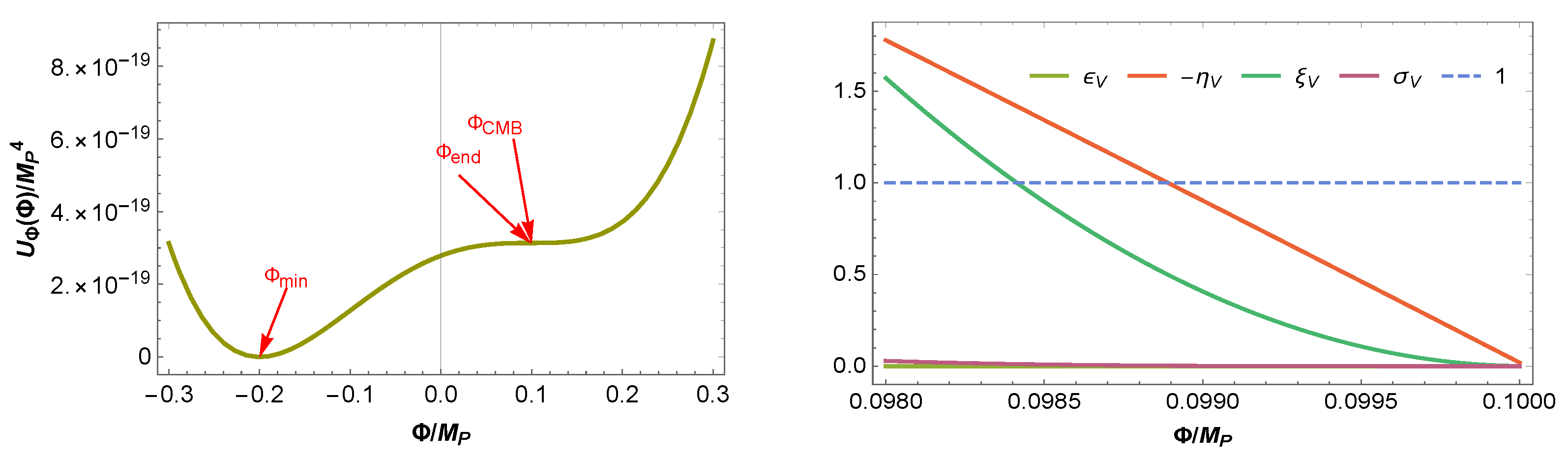
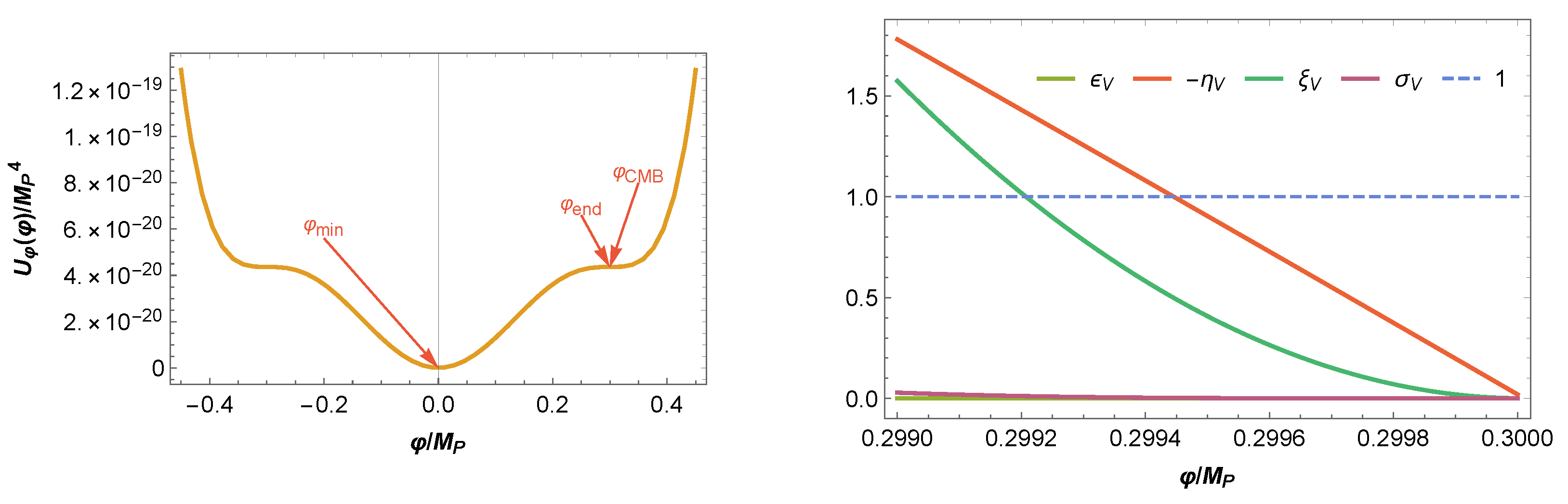
• For the inflationary epoch, we assumed slow roll single field inflation minimally coupled to gravity. For the inflaton potential, we considered two polynomial potentials, each of which possesses an inflection point. Forbye, the potential of Model II is not symmetric about the origin. Contrarily, the potential of Model I is not symmetric under the transformation of $\mathsf{\Phi }\to -\mathsf{\Phi }$ (see Equations (2) and (3)).
• After fixing the coefficients of the potentials using the current CMB data for near-inflection point inflationary scenario, we found $n_s$∼ 0.96, r∼${10}^{-12}$ (see Table 2 and Table 3).
• We assumed that inflaton decays to SM Higgs (H) together with DM $\left(\chi \right)$. We determined the upper bounds of the couplings as ${\lambda }_{12}/M_P\lesssim \mathcal{O}\left({10}^{-12}\right)$ and $y_{\chi }\lesssim \mathcal{O}\left({10}^{-6}\right)$ from stability analysis of the inflation-potential. The previous upper bound specifies the maximum allowed value of $T_{rh}$.
• Under the assumption of a near-inflection point scenario, we are forced to choose the CMB scale around the vicinity of the inflection point. Thus, the inflection point determines the CMB observables, such as $n_s$ and r on one hand, and controls the production of DM relic on the other hand.
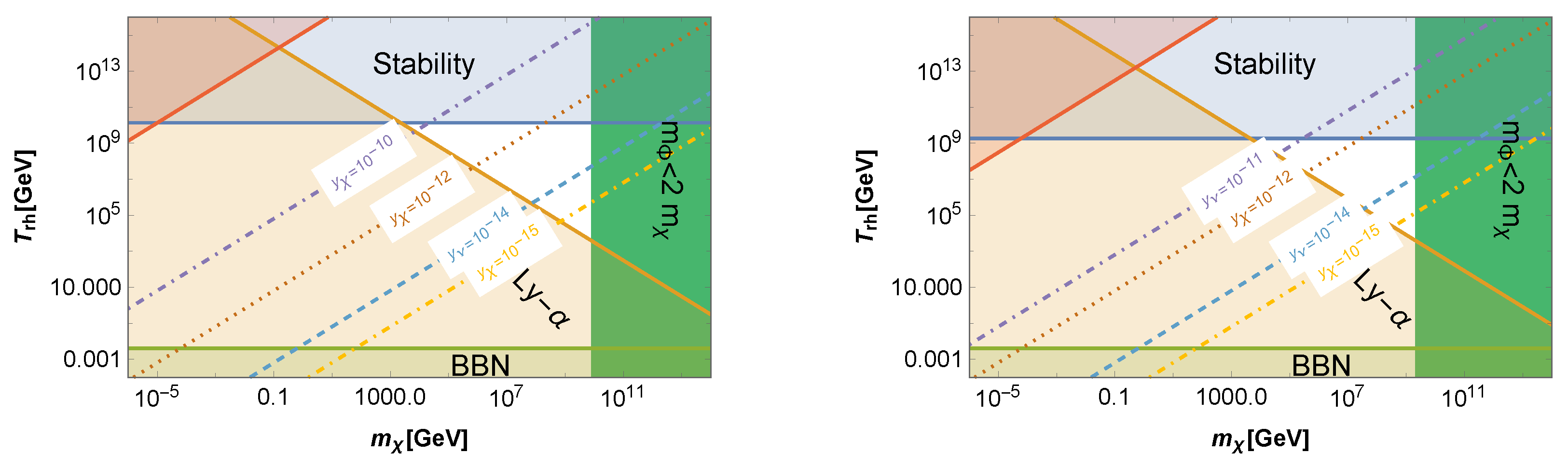
• We can infer that the total density of CDM in the contemporary universe can be explained if $\chi$ is produced only via the decay channel of inflaton. However, to do that the permissible range of $y_{\chi }$ and $m_{\chi }$ are $\mathcal{O}\left({10}^{-10}\right)\gtrsim y_{\chi }\gtrsim \mathcal{O}\left({10}^{-15}\right)$ (for $2.5\times {10}^3\mathrm{GeV}\lesssim m_{\chi }\lesssim 8.1\times {10}^9\mathrm{GeV}$ in Model I) and $\mathcal{O}\left({10}^{-11}\right)\gtrsim y_{\chi }\gtrsim \mathcal{O}\left({10}^{-15}\right)$ (for $8.4\times {10}^3\mathrm{GeV}\lesssim m_{\chi }\lesssim 2\times {10}^9\mathrm{GeV}$ in Model II). This is illustrated on $(T_{rh},m_{\chi })$ plane in Figure 3. The other cosmological bounds on that plane are coming from BBN temperature (should be $\gtrsim 4\mathrm{MeV}$), stability analysis of the inflationary potential from radiative correction, Ly-$\alpha$ bound so that $\chi$ is no longer warm dark matter in the present universe, and the maximum value of $m_{\chi }$ should be $\lesssim m_{\mathsf{\Phi }\left(\phi \right)}$.
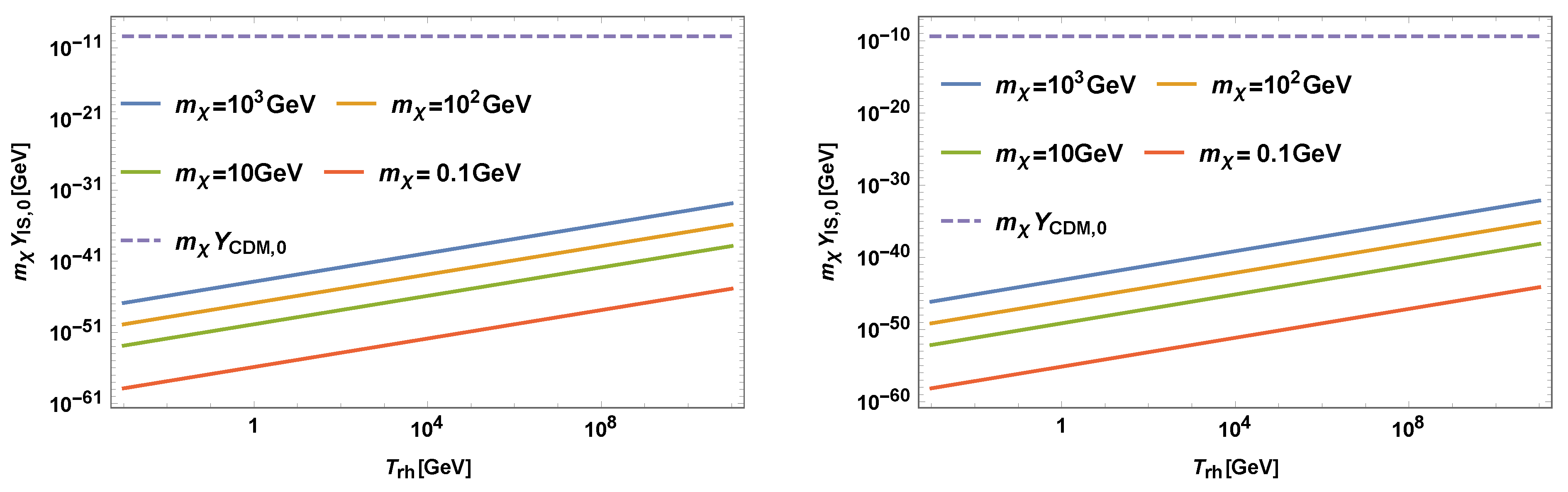
• We also discussed three 2-to-2 scattering channels of either SM particles or inflatons, which can produce significant amount of $\chi$ via scattering. However, all of these scattering processes can contribute only a negligible fraction of $Y_{\mathrm{CDM},0}$.

This work aimed to address the dark matter puzzle of the Universe and to connect it with cosmological inflation, as well as satisfy the combined constraints coming from different observations. Future measurements of the CMB from experiments like CMB-S4, SPTpol, LiteBIRD, and other such experiments will further be able to test the simple models we have presented.

References

1. Aghanim, N.; Akrami, Y.; Ashdown, M.; Aumont, J.; Baccigalupi, C.; Ballardini, M.; Bay, A.J.; Barreiro, R.B.; Bartolo, N.; Basak, S.; et al. Planck 2018 results. VI. Cosmological parameters. Astron. Astrophys. 2020, 641, A6, Erratum in Astron. Astrophys. 2021, 652, C4. [Google Scholar] [CrossRef] [Green Version]
2. Ade, P.A.R.; Ahmed, Z.; Amiri, M.; Barkats, D.; Thakur, R.B.; Bischoff, C.A.; Beck, D.; Bock, J.J.; Boenish, H.; Bullock, E.; et al. Improved Constraints on Primordial Gravitational Waves using Planck, WMAP, and BICEP/Keck Observations through the 2018 Observing Season. Phys. Rev. Lett. 2021, 127, 151301. [Google Scholar] [CrossRef] [PubMed]
3. Starobinsky, A.A. A New Type of Isotropic Cosmological Models Without Singularity. Phys. Lett. B 1980, 91, 99–102. [Google Scholar] [CrossRef]
4. Guth, A.H. The Inflationary Universe: A Possible Solution to the Horizon and Flatness Problems. Phys. Rev. D 1981, 23, 347–356. [Google Scholar] [CrossRef] [Green Version]
5. Linde, A.D. A New Inflationary Universe Scenario: A Possible Solution of the Horizon, Flatness, Homogeneity, Isotropy and Primordial Monopole Problems. Phys. Lett. B 1982, 108, 389–393. [Google Scholar] [CrossRef]
6. Martin, J.; Ringeval, C.; Vennin, V. Encyclopædia Inflationaris. Phys. Dark Univ. 2014, 5–6, 75–235. [Google Scholar] [CrossRef] [Green Version]
7. Albrecht, A.; Steinhardt, P.J.; Turner, M.S.; Wilczek, F. Reheating an Inflationary Universe. Phys. Rev. Lett. 1982, 48, 1437. [Google Scholar] [CrossRef]
8. Dolgov, A.D.; Kirilova, D.P. On particle creation by a time dependent scalar field. Sov. J. Nucl. Phys. 1990, 51, 172–177. [Google Scholar]
9. Traschen, J.H.; Brandenberger, R.H. Particle Production During Out-of-equilibrium Phase Transitions. Phys. Rev. D 1990, 42, 2491–2504. [Google Scholar] [CrossRef]
10. Shtanov, Y.; Traschen, J.H.; Brandenberger, R.H. Universe reheating after inflation. Phys. Rev. D 1995, 51, 5438–5455. [Google Scholar] [CrossRef] [Green Version]
11. Kofman, L.; Linde, A.D.; Starobinsky, A.A. Reheating after inflation. Phys. Rev. Lett. 1994, 73, 3195–3198. [Google Scholar] [CrossRef] [Green Version]
12. Boyanovsky, D.; de Vega, H.J.; Holman, R.; Salgado, J.F.J. Analytic and numerical study of preheating dynamics. Phys. Rev. D 1996, 54, 7570–7598. [Google Scholar] [CrossRef] [PubMed] [Green Version]
13. Kofman, L.; Linde, A.D.; Starobinsky, A.A. Towards the theory of reheating after inflation. Phys. Rev. D 1997, 56, 3258–3295. [Google Scholar] [CrossRef] [Green Version]
14. Caprini, C.; Figueroa, D.G. Cosmological Backgrounds of Gravitational Waves. Class. Quant. Grav. 2018, 35, 163001. [Google Scholar] [CrossRef] [Green Version]
15. Martin, J.; Ringeval, C. First CMB Constraints on the Inflationary Reheating Temperature. Phys. Rev. D 2010, 82, 23511. [Google Scholar] [CrossRef] [Green Version]
16. Adshead, P.; Easther, R.; Pritchard, J.; Loeb, A. Inflation and the Scale Dependent Spectral Index: Prospects and Strategies. JCAP 2011, 2, 21. [Google Scholar] [CrossRef] [Green Version]
17. Easther, R.; Peiris, H.V. Bayesian Analysis of Inflation II: Model Selection and Constraints on Reheating. Phys. Rev. D 2012, 85, 103533. [Google Scholar] [CrossRef] [Green Version]
18. Martin, J.; Ringeval, C.; Vennin, V. Observing Inflationary Reheating. Phys. Rev. Lett. 2015, 114, 081303. [Google Scholar] [CrossRef] [Green Version]
19. Munoz, J.B.; Kamionkowski, M. Equation-of-State Parameter for Reheating. Phys. Rev. D 2015, 91, 043521. [Google Scholar] [CrossRef] [Green Version]
20. Cook, J.L.; Dimastrogiovanni, E.; Easson, D.A.; Krauss, L.M. Reheating predictions in single field inflation. JCAP 2015, 4, 47. [Google Scholar] [CrossRef]
21. Zhang, N.; Wu, Y.B.; Lu, J.W.; Sun, C.W.; Shou, L.J.; Xu, H.Z. Constraints on the generalized natural inflation after Planck 2018. Chin. Phys. C 2020, 44, 95107. [Google Scholar] [CrossRef]
22. Stein, N.K.; Kinney, W.H. Natural inflation after Planck 2018. JCAP 2022, 1, 22. [Google Scholar] [CrossRef]
23. Cai, R.G.; Guo, Z.K.; Wang, S.J. Reheating phase diagram for single-field slow-roll inflationary models. Phys. Rev. D 2015, 92, 063506. [Google Scholar] [CrossRef] [Green Version]
24. Marco, A.D.; Pradisi, G.; Cabella, P. Inflationary scale, reheating scale, and pre-BBN cosmology with scalar fields. Phys. Rev. D 2018, 98, 123511. [Google Scholar] [CrossRef] [Green Version]
25. Maity, D.; Saha, P. (P)reheating after minimal Plateau Inflation and constraints from CMB. JCAP 2019, 7, 018. [Google Scholar] [CrossRef] [Green Version]
26. Maity, D.; Saha, P. Minimal plateau inflationary cosmologies and constraints from reheating. Class. Quant. Grav. 2019, 36, 045010. [Google Scholar] [CrossRef] [Green Version]
27. Antusch, S.; Figueroa, D.G.; Marschall, K.; Torrenti, F. Energy distribution and equation of state of the early Universe: Matching the end of inflation and the onset of radiation domination. Phys. Lett. B 2020, 811, 135888. [Google Scholar] [CrossRef]
28. Dai, L.; Kamionkowski, M.; Wang, J. Reheating constraints to inflationary models. Phys. Rev. Lett. 2014, 113, 041302. [Google Scholar] [CrossRef] [Green Version]
29. Domcke, V.; Heisig, J. Constraints on the reheating temperature from sizable tensor modes. Phys. Rev. D 2015, 92, 103515. [Google Scholar] [CrossRef] [Green Version]
30. Dalianis, I.; Koutsoumbas, G.; Ntrekis, K.; Papantonopoulos, E. Reheating predictions in Gravity Theories with Derivative Coupling. JCAP 2017, 2, 27. [Google Scholar] [CrossRef]
31. Takahashi, F.; Yin, W. ALP inflation and Big Bang on Earth. JHEP 2019, 7, 095. [Google Scholar] [CrossRef] [Green Version]
32. Hardwick, R.J.; Vennin, V.; Koyama, K.; Wands, D. Constraining Curvatonic Reheating. JCAP 2016, 8, 042. [Google Scholar] [CrossRef] [Green Version]
33. Ueno, Y.; Yamamoto, K. Constraints on α-attractor inflation and reheating. Phys. Rev. D 2016, 93, 083524. [Google Scholar] [CrossRef] [Green Version]
34. Nozari, K.; Rashidi, N. Perturbation, non-Gaussianity, and reheating in a Gauss-Bonnet α-attractor model. Phys. Rev. D 2017, 95, 123518. [Google Scholar] [CrossRef] [Green Version]
35. Marco, A.D.; Cabella, P.; Vittorio, N. Constraining the general reheating phase in the α-attractor inflationary cosmology. Phys. Rev. D 2017, 95, 103502. [Google Scholar] [CrossRef] [Green Version]
36. Drewes, M.; Kang, J.U.; Mun, U.R. CMB constraints on the inflaton couplings and reheating temperature in α-attractor inflation. JHEP 2017, 11, 72. [Google Scholar] [CrossRef] [Green Version]
37. Maity, D.; Saha, P. Connecting CMB anisotropy and cold dark matter phenomenology via reheating. Phys. Rev. D 2018, 98, 103525. [Google Scholar] [CrossRef] [Green Version]
38. Rashidi, N.; Nozari, K. α-Attractor and reheating in a model with noncanonical scalar fields. Int. J. Mod. Phys. D 2018, 27, 1850076. [Google Scholar] [CrossRef]
39. Mishra, S.S.; Sahni, V.; Starobinsky, A.A. Curing inflationary degeneracies using reheating predictions and relic gravitational waves. JCAP 2021, 5, 75. [Google Scholar] [CrossRef]
40. Ellis, J.; Garcia, M.A.G.; Nanopoulos, D.V.; Olive, K.A.; Verner, S. BICEP/Keck constraints on attractor models of inflation and reheating. Phys. Rev. D 2022, 105, 043504. [Google Scholar] [CrossRef]
41. Nautiyal, A. Reheating constraints on Tachyon Inflation. Phys. Rev. D 2018, 98, 103531. [Google Scholar] [CrossRef] [Green Version]
42. Choi, S.M.; Lee, H.M. Inflection point inflation and reheating. Eur. Phys. J. C 2016, 76, 303. [Google Scholar] [CrossRef] [Green Version]
43. Cabella, P.; Marco, A.D.; Pradisi, G. Fiber inflation and reheating. Phys. Rev. D 2017, 95, 123528. [Google Scholar] [CrossRef] [Green Version]
44. Kabir, R.; Mukherjee, A.; Lohiya, D. Reheating constraints on Kähler moduli inflation. Mod. Phys. Lett. A 2019, 34, 1950114. [Google Scholar] [CrossRef] [Green Version]
45. Bhattacharya, S.; Dutta, K.; Maharana, A. Constraints on Kähler moduli inflation from reheating. Phys. Rev. D 2017, 96, 083522. [Google Scholar] [CrossRef] [Green Version]
46. Dalianis, I.; Watanabe, Y. Probing the BSM physics with CMB precision cosmology: An application to supersymmetry. JHEP 2018, 2, 118. [Google Scholar] [CrossRef] [Green Version]
47. Szydagis, M.; Balajthy, J.; Block, G.A.; Brodsky, J.P.; Brown, E.; Cutter, J.E.; Farrell, S.J.; Huang, J.; Kozlova, E.S.; Liebenthal, C.S.; et al. A Review of NEST Models, and Their Application to Improvement of Particle Identification in Liquid Xenon Experiments. arXiv 2022, arXiv:2211.10726. [Google Scholar]
48. Baudis, L.; Hall, J.; Lesko, K.T.; Orrell, J.L. Snowmass 2021 Underground Facilities and Infrastructure Overview Topical Report. arXiv 2022, arXiv:2212.07037. [Google Scholar]
49. Hall, L.J.; Jedamzik, K.; March-Russell, J.; West, S.M. Freeze-In Production of FIMP Dark Matter. JHEP 2010, 3, 080. [Google Scholar] [CrossRef] [Green Version]
50. Ade, P.A.R.; Ahmed, Z.; Amiri, M.; Barkats, D.; Thakur, R.B.; Beck, D.; Bischoff, C.; Bock, J.J.; Boenish, H.; Bullock, E.; et al. The Latest Constraints on Inflationary B-modes from the BICEP/Keck Telescopes. arXiv 2022, arXiv:2203.16556. [Google Scholar]
51. Ghoshal, A.; Lambiase, G.; Pal, S.; Paul, A.; Porey, S. Inflection-point inflation and dark matter redux. JHEP 2022, 9, 231. [Google Scholar] [CrossRef]
52. Bernal, N.; Xu, Y. Polynomial inflation and dark matter. Eur. Phys. J. C 2021, 81, 877. [Google Scholar] [CrossRef]
53. Drees, M.; Xu, Y. Small field polynomial inflation: Reheating, radiative stability and lower bound. JCAP 2021, 9, 012. [Google Scholar] [CrossRef]
54. Campeti, P.; Komatsu, E. New Constraint on the Tensor-to-scalar Ratio from the Planck and BICEP/Keck Array Data Using the Profile Likelihood. Astrophys. J. 2022, 941, 110. [Google Scholar] [CrossRef]
55. Okada, N.; Raut, D. Inflection-point Higgs Inflation. Phys. Rev. D 2017, 95, 035035. [Google Scholar] [CrossRef] [Green Version]
56. Dimopoulos, K. Ultra slow-roll inflation demystified. Phys. Lett. B 2017, 775, 262–265. [Google Scholar] [CrossRef]
57. Hotchkiss, S.; Mazumdar, A.; Nadathur, S. Observable gravitational waves from inflation with small field excursions. JCAP 2012, 2, 8. [Google Scholar] [CrossRef] [Green Version]
58. Chatterjee, A.; Mazumdar, A. Bound on largest r≲0.1 from sub-Planckian excursions of inflaton. JCAP 2015, 1, 31. [Google Scholar] [CrossRef] [Green Version]
59. Garcia-Bellido, J.; Morales, E.R. Primordial black holes from single field models of inflation. Phys. Dark Univ. 2017, 18, 47–54. [Google Scholar] [CrossRef] [Green Version]
60. Okada, N.; Okada, S.; Raut, D. Inflection-point inflation in hyper-charge oriented U(1)X model. Phys. Rev. D 2017, 95, 055030. [Google Scholar] [CrossRef] [Green Version]
61. Zyla, P.A.; Barnett, R.M.; Beringer, J.; Dahl, O.; Dwyer, D.A.; Groom, D.E.; Lin, C.-J.; Lugovsky, K.S.; Pianori, E.; Robinson, D.J.; et al. Review of Particle Physics. PTEP 2020, 2020, 083C01. [Google Scholar] [CrossRef]
62. Ghoshal, A.; Lambiase, G.; Pal, S.; Paul, A.; Porey, S. Near-inflection point inflation and production of dark matter during reheating. arXiv 2022, arXiv:2211.15061. [Google Scholar]
63. Giudice, G.F.; Kolb, E.W.; Riotto, A. Largest temperature of the radiation era and its cosmological implications. Phys. Rev. D 2001, 64, 023508. [Google Scholar] [CrossRef] [Green Version]
64. Hasegawa, T.; Hiroshima, N.; Kohri, K.; Hansen, R.S.L.; Tram, T.; Hannestad, S. MeV-scale reheating temperature and thermalization of oscillating neutrinos by radiative and hadronic decays of massive particles. JCAP 2019, 12, 012. [Google Scholar] [CrossRef] [Green Version]
65. Kawasaki, M.; Kohri, K.; Sugiyama, N. Cosmological constraints on late time entropy production. Phys. Rev. Lett. 1999, 82, 4168. [Google Scholar] [CrossRef] [Green Version]
66. Kawasaki, M.; Kohri, K.; Sugiyama, N. MeV scale reheating temperature and thermalization of neutrino background. Phys. Rev. D 2000, 62, 023506. [Google Scholar] [CrossRef] [Green Version]
Figure 1. The left panel presents the inflaton-potential of Model I inflation for benchmark value from Table 2, and the right panel shows potential-slow-roll parameters ϵ V , η V , ξ V , and σ V . The horizontal dashed line stands for 1.
Symmetry 15 00543 g001
Figure 2. Inflaton-potential (left panel) of Model II for the benchmark value from Table 3, and the absolute values of four potential slow roll parameters ( ϵ V , η V , ξ V , σ V ) as a function of φ / M P . The dashed line specifies the value 1.
Symmetry 15 00543 g002
Figure 3. The unshaded triangular region on the ( T r h , m χ ) plane indicates the allowed region: Left panel is for Model I, whereas right panel is for Model II. The colored zones are coming from different bounds: (a) the horizontal stripe of light green color: T r h should be more than 4 MeV (Big Bang Nucleosynthesis (BBN) temperature) [63] (see also [64,65,66]), (b) the horizontal stripe of blue color: from the maximum permissible value of λ 12 from the stability analysis of Section 3, (c) the light pink colored region in the top-left corner: from the allowed maximum value of y χ from the stability analysis of Section 3, (d) the green (medium sea green) colored vertical strip on right from the maximum possible value of m χ ( m χ must be < m Φ ( φ ) / 2 ), (e) the peach (peach puff) colored region shows bound from Ly- α estimation : T r h ( 2 m Φ ) / m χ or T r h ( 2 m φ ) / m χ [52]. The diagonal discontinuous lines correspond to different values of y χ and represent the allowed range of y χ satisfying present-day CDM yield, provided that χ is produced solely from the decay channel of inflation during the reheating era.
Symmetry 15 00543 g003
Figure 4. Comparison of m χ × Y I S , 0 (continuous lines) for different values of m χ with m χ × Y CDM , 0 (dashed horizontal line) for Model I in the left panel and for Model II inflation in the right panel.
Symmetry 15 00543 g004