Modelling and Analysis of a Measles Epidemic Model with the Constant Proportional Caputo Operator

Abstract

Despite the existence of a secure and reliable immunization, measles, also known as rubeola, continues to be a leading cause of fatalities globally, especially in underdeveloped nations. For investigation and observation of the dynamical transmission of the disease with the influence of vaccination, we proposed a novel fractional order measles model with a constant proportional (CP) Caputo operator. We analysed the proposed model’s positivity, boundedness, well-posedness, and biological viability. Reproductive and strength numbers were also verified to examine how the illness dynamically behaves in society. For local and global stability analysis, we introduced the Lyapunov function with first and second derivatives. In order to evaluate the fractional integral operator, we used different techniques to invert the PC and CPC operators. We also used our suggested model’s fractional differential equations to derive the eigenfunctions of the CPC operator. There is a detailed discussion of additional analysis on the CPC and Hilfer generalised proportional operators. Employing the Laplace with the Adomian decomposition technique, we simulated a system of fractional differential equations numerically. Finally, numerical results and simulations were derived with the proposed measles model. The intricate and vital study of systems with symmetry is one of the many applications of contemporary fractional mathematical control. A strong tool that makes it possible to create numerical answers to a given fractional differential equation methodically is symmetry analysis. It is discovered that the proposed fractional order model provides a more realistic way of understanding the dynamics of a measles epidemic.

1. Introduction

Despite the fact that there is a reliable and efficient vaccine, measles, also known as rubeola, is still a major cause of death globally, particularly in developing nations. Measles is a contagious viral infection brought on by the “Paramyxovirus”, a member of the Morbillivirus genus in the Paramyxoviridae family [1]. Children under the age of five are disproportionately affected, and in 2017, measles claimed the lives of around 110,000 individuals, primarily young children under the age of six [2]. After first affecting the respiratory system, the measles virus slowly spreads through the bloodstream to other bodily organs. High fever, a runny or blocked nose, sneezing, sore (or red) eyes, a cough, and rashes are some of the early signs of measles. The rash typically develops a few days after the cold-like symptoms. Measles infections have some serious complications such as severe diarrhea, dehydration, pneumonia, blindness, malnutrition, lung infection, loss of immunity, nervous system damage, or even death [3]. Measles is highly contagious, and the infection can spread very easily from one person to another. An infected person is contagious for approximately 4 days before a significant rash appears. Furthermore, even after the rash appears, they are still contagious for another four days. The risk of complications from measles infection continues to be higher in those who have not received the vaccine, in children, in those with compromised immune systems, and in pregnant women [4]. Vaccination is an effective disease-prevention strategy; therefore, a framework that optimises vaccine coverage levels to halt disease spread is required. In mathematical modeling, we investigate model construction, parameter estimation, model sensitivity to various parameters, and numerical simulations [5]. Mathematical models are used to describe and solve specific issues for the disease under consideration. These mathematical models help us capture the growth in diseases and provide various techniques to control their propagation. In recent years, numerous mathematical models have been developed to investigate the dynamics of measles transmission [6,7,8,9,10].

Researchers’ interest in the idea of fractional calculus has grown recently. In many fields of mathematics, engineering, and biology, numerous applications of fractional calculus can be found in the explanation of intricate dynamical systems with memory effects [11,12,13,14]. The most noticeable characteristic of fractional differential equations is that they distinguish between the genetic and memory characteristics of distinct mathematical models. Therefore, compared to the traditional integer order models, fractional order models seem to be more factual and empirical. For the semantic and profane propagation of measles in metapopulations, Goufo et al. [15] suggested a fractional order SEIR epidemic model. A non-singular fractional derivative-based fractional dynamical analysis of a measles outbreak under vaccination was reported by G. Nazir et al. [16]. Farman et al. [17] developed and provided a numerical solution of an SEIR epidemic model with non-integer temporal fractional derivatives to control measles in infected populations. Ogunmiloro et al. [18] investigated two groups of measles-infected and measles-induced encephalitis-infected people with recurrence under the Atangana–Baleanu–Caputo (ABC) fractional operator, explaining measles propagation dynamics with a double dose of vaccination. Using the Caputo fractional derivative, Qureshi built an epidemiological model for a measles epidemic [19]. Numerous studies have employed fractional order derivatives to study the kinetics of measles transmission [20,21,22,23]. Fractional-order mathematical models of a few more infectious diseases have recently been studied in [24,25,26,27].

In order to examine the critical normal form coefficients of bifurcations for both one-parameter and two-parameter bifurcations, a Lotka–Volterra model was discretised using a recently revealed nonstandard finite difference method [28]. Currently, COVID-19 is a widespread infection that is difficult to treat. In their research, Xu et al. [29] used innovative operators to observe the impact of vaccination in a COVID-19 model, with a range of meaningful parameter values that were used to demonstrate the impact of vaccination. The Lyapunov approach is one of the most reliable and efficient techniques for analyzing the stability characteristics of solutions [30]. Researchers have studied many sorts of stability for fractional differential equations using various fractional derivatives of Lyapunov functions [31,32]. The Laplace Adomain decomposition method, which is a potent technique, is the result of the coupling of ADM with the Laplace transform (LADM). Differential equations are transformed into algebraic equations with the use of the Laplace transform, and nonlinear factors are then decomposed into Adomain polynomials. This numerical technique effectively solves a set of stochastic differential equations in addition to deterministic differential equations. More specifically, it may be applied to a system of fractional order equations as well as classically ordered ordinary and partial differential equations that are linear and nonlinear. This approach does not need to be one of perturbation or liberalization. Furthermore, unlike RK4, it does not require a set step size. LADM is more effective than the normal approach, as the authors highlight in [33,34,35]. The CPC operator is more general than Caputo’s fractional derivative operator. Sweilam et al. [36] investigated a fractional order COVID-19 model with the CPC operator and discovered that offered approaches with the CPC operator outperform proposed methods with the Caputo operator. Researchers studied a HIV pandemic fractional model using the Caputo operator and the constant proportional Caputo (CPC) operator in [37]. They discovered that the differential transformation approach and the Laplace Adomian decomposition method are useful in producing approximation findings for the model studied in this paper. When compared to DTM, LADM produces more consistent outcomes. The method used in this work is a novel fractional order SVEIHR model to examine measles dynamics.

The structure of the current paper is as follows: An introduction and a review of the literature are presented in Section 1. In Section 2, we discuss the fundamentals of the fractional operator used in the model. In Section 3, we propose a fractional order model on transmission dynamics of measles and discuss the positiveness and boundedness of the solutions, the feasible region, the well-posedness, the strength number $A_0$, an analysis of equilibrium points, and also examine the local and global asymptotic stability of the fractional order model using the Lyapunov function first and second derivatives. Section 4 consists of a detailed analysis of the proposed model using the hybrid fractional operator CPC. In Section 5, we derive the solution to the proposed system of fractional differential using the LADM method. In Section 6, the numerical simulations and modeling of the proposed scheme are shown graphically, and we give an interpretations of the figures to check the conduct of the disease. The main conclusions of our analysis are covered in Section 7.

2. Preliminaries

Here, we discuss some primary definitions that are useful to analyze the system.

Definition 1.

For $\gamma >0$ and any integrable function $\theta \left(t\right)$, the RLF integral of order γ can be stated as [38]:

$${}_a^{RL}{I}_t^{\gamma }\theta \left(t\right)=\frac{1}{\Gamma \left(\gamma \right)}{\int }_a^t\theta \left(\eta \right){(t-\eta )}^{\gamma -1}d\eta ,-\infty \le a<t\le \infty$$

(1)

Definition 2.

In [39], a subsequent operator for generalised non-fractional differentials, often known as proportional or conformable, was defined as:

$$\begin{array}{c}\hfill {}^P{D}_t^{\gamma }\theta \left(t\right)=K_1(\gamma ,t)\theta \left(t\right)+K_0\left(\gamma ,t\right){\theta }^{\prime }\left(t\right)\end{array}$$

(2)

Here, we use the specific case

$$\begin{array}{c}\hfill K_0(\gamma ,t)=\gamma t^{1-\gamma },K_1(\gamma ,t)=(1-\gamma )t^{\gamma }\end{array}$$

(3)

where $K_0$ and $K_1$ are functions of t and $\gamma \in [0,1]$, which fulfil the following criterion for all $t\in \mathbb{R}$:

$$\underset{\gamma \to 0^{+}}{lim}{K}_0(\gamma ,t)=0,\underset{\gamma \to 1^{-}}{lim}{K}_0(\gamma ,t)=1,K_0(\gamma ,t)\ne 0,\gamma \in (0,1]$$

(4)

$$\underset{\gamma \to 0^{+}}{lim}{K}_1(\gamma ,t)=1,\underset{\gamma \to 1^{-}}{lim}{K}_1(\gamma ,t)=0,K_1(\gamma ,t)\ne 0,\gamma \in [0,1)$$

(5)

This may be viewed as a generalization of standard differential operator $D\theta \left(t\right)={\theta }^{\prime }\left(t\right)$, dependent on γ, which is helpful in regulatory theory [39]. Furthermore, a special case may be interesting for us, where the functions $K_0$ and $K_1$ are depending only on γ, known as a constant proportional (CP) operator and defined as:

$${}^{CP}{D}_t^{\gamma }=K_1\left(\gamma \right)\theta \left(t\right)+K_0\left(\gamma \right){\theta }^{\prime }\left(t\right)$$

(6)

Definition 3.

In [38], a hybrid fractional operator, known as proportional Caputo (PC), was proposed by combining the proportional operator and the Caputo fractional derivative:

$$\begin{array}{ccc}\hfill {}_0^{PC}{D}_t^{\gamma }\theta \left(t\right)& =& \frac{1}{\Gamma (1-\gamma )}{\int }_0^t\left(K_1(\gamma ,\eta )\theta \left(\eta \right)+K_0\left(\gamma ,\eta \right){\theta }^{\prime }\left(\eta \right)\right){(t-\eta )}^{-\gamma }d\eta \hfill \end{array}$$

(7)

$$\begin{array}{ccc}& =& {}_0^{RL}{I}_t^{1-\gamma }\left[K_1(\gamma ,t)\theta \left(t\right)+K_0\left(\gamma ,t\right){\theta }^{\prime }\left(t\right)\right]\hfill \end{array}$$

(8)

Consider a specific case where $K_0$ and $K_1$ are independent of t as in the ${}^{CP}{D}_{\gamma }$, known as the constant proportional Caputo (CPC) operator, and defined as follows:

$$\begin{array}{ccc}\hfill {}_0^{CPC}{D}_t^{\gamma }\theta \left(t\right)& =& \frac{1}{\Gamma (1-\gamma )}{\int }_0^t\left(K_1\left(\gamma \right)\theta \left(\eta \right)+K_0\left(\gamma \right){\theta }^{\prime }\left(\eta \right)\right){(t-\eta )}^{-\gamma }d\eta \hfill \end{array}$$

(9)

$$\begin{array}{ccc}& =& K_1\left(\gamma \right){}_0^{RL}{I}_t^{1-\gamma }\theta \left(t\right)+K_0\left(\gamma \right){}_0^C{D}_t^{\gamma }\theta \left(t\right)\hfill \end{array}$$

(10)

3. Fractional Order Model on Transmission Dynamics of Measles

Here, we present a time fractional order scheme of measles transmission dynamics. Measles transmission dynamics are mathematically modeled in [10] using a deterministic approach. The model splits the number of people into six groups, including susceptible $\mathcal{S}\left(t\right)$, vaccinated $\mathcal{V}\left(t\right)$, exposed $\mathcal{E}\left(t\right)$, infected $\mathcal{I}\left(t\right)$, hospitalised $\mathcal{H}\left(t\right)$, and recovered $\mathcal{R}\left(t\right)$, based on each person’s epidemiological state. There is a rate, $\varphi$, of recruitment of the susceptible class on a daily basis. People in the susceptible class get vaccinated at a certain rate, $\pi$, and lose immunity at a certain rate, $\omega$, as their immunity from the vaccine wanes. The rate at which the exposed class becomes the infected class is $\beta$, $\alpha$ is the rate at which vulnerable individuals are infected, and $\alpha \mathcal{S}\mathcal{I}$ is the force of infection. When measles complications arise, infected people attend the hospital at a rate $\rho$, and when they receive treatment, they recover from the illness at a rate $\gamma$. All classes experience a natural death at a rate of $\mu$, and measles-related mortality is shown by $\delta$. In this study, the rate of measles curing naturally has not been taken into account. The aforementioned description may be expressed as a set of time fractional order differential equations:

$$\left\{\begin{array}{c}{}_0^{CPC}{D}_t^{\gamma }\mathcal{S}\left(t\right)=\varphi -\alpha \mathcal{SI}+\omega \mathcal{V}-q_1\mathcal{S}\hfill \\ {}_0^{CPC}{D}_t^{\gamma }\mathcal{V}\left(t\right)=\pi \mathcal{S}-q_2\mathcal{V}\hfill \\ {}_0^{CPC}{D}_t^{\gamma }\mathcal{E}\left(t\right)=\alpha \mathcal{SI}-q_3\mathcal{E}\hfill \\ {}_0^{CPC}{D}_t^{\gamma }\mathcal{I}\left(t\right)=\beta \mathcal{E}-q_4\mathcal{I}\hfill \\ {}_0^{CPC}{D}_t^{\gamma }\mathcal{H}\left(t\right)=\rho \mathcal{I}-q_5\mathcal{H}\hfill \\ {}_0^{CPC}{D}_t^{\gamma }\mathcal{R}\left(t\right)=\sigma \mathcal{H}-\mu \mathcal{R}\hfill \end{array}\right.$$

(11)

where $q_1=(\pi +\mu )$, $q_2=(\mu +\omega )$, $q_3=(\mu +\beta )$, $q_4=(\mu +\delta +\rho )$, and $q_5=(\sigma +\delta +\mu )$, with non-negative initial constraints,

$$\begin{array}{c}\hfill \mathcal{S}\left(0\right)={\mathcal{S}}_0,\mathcal{V}\left(0\right)={\mathcal{V}}_0,\mathcal{E}\left(0\right)={\mathcal{E}}_0,\mathcal{I}\left(0\right)={\mathcal{I}}_0,\mathcal{H}\left(0\right)={\mathcal{H}}_0,\mathcal{R}\left(0\right)={\mathcal{R}}_0\end{array}$$

(12)

3.1. Positiveness and Boundness of Solutions

In this part, we investigate the factors that ensure the model’s solutions are positive. We begin with $\mathcal{V}\left(t\right)$:

$$\mathcal{V}\left(t\right)\ge {\mathcal{V}}_0{e}^{-q_{2}t},\forall t>0$$

(13)

and similarly, we have following inequalities:

$$\begin{array}{ccc}\hfill \mathcal{E}\left(t\right)\ge {\mathcal{E}}_0{e}^{-q_{3}t}& ,& \mathcal{I}\left(t\right)\ge {\mathcal{I}}_0{e}^{-q_{4}t},\forall t>0\hfill \end{array}$$

(14)

$$\begin{array}{ccc}\hfill \mathcal{H}\left(t\right)\ge {\mathcal{H}}_0{e}^{-q_{5}t}& ,& \mathcal{R}\left(t\right)\ge {\mathcal{R}}_0{e}^{-\left(\mu \right)t},\forall t>0\hfill \end{array}$$

(15)

The definition of the norm is:

$${\Vert \lambda \Vert }_{\infty }={sup}_{t\in D_{\lambda }}\left|\lambda \left(t\right)\right|$$

(16)

We obtain the function’s subsequent inequality, $\mathcal{S}\left(t\right)$, using this norm:

$$\begin{array}{ccc}\hfill {}_0^{CPC}{D}_t^{\gamma }\mathcal{S}\left(t\right)& =& \varphi -\alpha \mathcal{SI}+\omega \mathcal{V}-q_1\mathcal{S},\forall t>0\hfill \\ & \ge & -\alpha \mathcal{SI}-q_1\mathcal{S}\ge -\left(\alpha \left|\mathcal{I}\right|+q_1\right)\mathcal{S},\forall t>0\hfill \\ & \ge & -\left(\alpha su{p}_{t\in D_I}\left|\mathcal{I}\right|+q_1\right)\mathcal{S}\ge -\left({\alpha \left|\mathcal{I}\right|}_{\infty }+q_1\right)\mathcal{S},\forall t>0\hfill \\ \hfill ⟹\mathcal{S}\left(t\right)& \ge & {\mathcal{S}}_0{e}^{-\left({\alpha \left|\mathcal{I}\right|}_{\infty }+q_1\right)t},\forall t>0\hfill \end{array}$$

(17)

3.2. Well-Posedness and Biological Feasibility

In this section, we examine the interval and region where the solution to our system makes historical sense. Let the entire population be $\mathcal{N}$ = $\mathcal{S}$ + $\mathcal{V}$ + $\mathcal{E}$ + $\mathcal{I}$ + $\mathcal{H}$ + $\mathcal{R}$, then:

$$\begin{array}{ccc}\hfill {}_0^{CPC}{D}_t^{\gamma }\mathcal{N}\left(t\right)& =& {}_0^{CPC}{D}_t^{\gamma }\mathcal{S}\left(t\right){+}_0^{CPC}{D}_t^{\gamma }\mathcal{V}\left(t\right){+}_0^{CPC}{D}_t^{\gamma }\mathcal{E}\left(t\right){+}_0^{CPC}{D}_t^{\gamma }\mathcal{I}\left(t\right){+}_0^{CPC}{D}_t^{\gamma }\mathcal{H}\left(t\right){+}_0^{CPC}{D}_t^{\gamma }\mathcal{R}\left(t\right)\hfill \\ & =& \varphi -\mu (\mathcal{S}+\mathcal{V}+\mathcal{E}+\mathcal{I}+\mathcal{H}+\mathcal{R})-\delta I-\delta H\hfill \\ & =& \varphi -\mu N-\delta I-\delta H\hfill \end{array}$$

In the absence of disease we have,

$${}_0^{CPC}{D}_t^{\gamma }\mathcal{N}\left(t\right)=\varphi -\mu N$$

It follows that:

$${}_0^{CPC}{D}_t^{\gamma }\mathcal{N}\left(t\right)\le 0\mathit{if}\mathcal{N}\left(t\right)\ge \frac{\varphi }{\mu },\forall t$$

(18)

and we can express this through a particular comparison principle

$$\mathcal{N}\left(t\right)\le \mathcal{N}\left(0\right)e^{-\mu t}+\frac{\varphi }{\mu }(1-e^{-\mu t})$$

(19)

Particularly,

$$\mathcal{N}\left(t\right)\le \frac{\varphi }{\mu }\mathit{if}\mathcal{N}\left(0\right)\le \frac{\varphi }{\mu }$$

(20)

This indicates that the feasible region can be used to study the model:

$$\Gamma =\{(\mathcal{S},\mathcal{V},\mathcal{E},\mathcal{I},\mathcal{H},\mathcal{R})\in {\mathbb{R}}_{+}^6:\mathcal{N}\le \frac{\varphi }{\mu }\}$$

(21)

3.3. Disease-Free Equilibrium

Disease-free equilibrium is when infection does not happen. Consequently, we set exposed $\left(\mathcal{E}\right)$, infected $\left(\mathcal{I}\right)$, and hospitalised $\left(\mathcal{H}\right)$ classes to zero in system (11), and hence the outcome provides the equilibrium of a disease-free state $\left(E_0\right)$ that are described as:

$$E_0=({\mathcal{S}}_0,{\mathcal{V}}_0,{\mathcal{E}}_0,{\mathcal{I}}_0,{\mathcal{H}}_0,{\mathcal{R}}_0)=\left(\frac{q_2\varphi }{(q_2+\pi )\mu },\frac{\varphi \pi }{(q_2+\pi )\mu },0,0,0,0\right)$$

(22)

3.4. Endemic Equilibrium

Infection leads to endemic equilibrium. Setting the right side equations of system (11) to zero yields the endemic equilibrium points, which are $E^{*}=({\mathcal{S}}^{*},{\mathcal{V}}^{*},{\mathcal{E}}^{*},{\mathcal{I}}^{*},{\mathcal{H}}^{*},{\mathcal{R}}^{*})$:

$$\left\{\begin{array}{c}{\mathcal{S}}^{*}=\frac{q_3{q}_4}{\alpha \beta },{\mathcal{I}}^{*}=\frac{\alpha \beta q_2\varphi -q_1{q}_2{q}_3{q}_4+q_3{q}_4\omega \pi }{\alpha q_2{q}_3{q}_4}\hfill \\ {\mathcal{V}}^{*}=\frac{\pi q_3{q}_4}{\alpha \beta q_2},{\mathcal{H}}^{*}=\frac{\rho \left(\alpha \beta q_2\varphi +q_3{q}_4\omega \pi -q_1{q}_2{q}_3{q}_4\right)}{\alpha q_2{q}_3{q}_4{q}_5}\hfill \\ {\mathcal{E}}^{*}=\frac{\alpha \beta q_2\varphi -q_1{q}_2{q}_3{q}_4+q_3{q}_4\omega \pi }{\alpha \beta q_2{q}_3},{\mathcal{R}}^{*}=\frac{\sigma \left(\alpha \beta q_3\varphi -q_1{q}_2{q}_3{q}_4+q_3{q}_4\omega \pi \right)}{\alpha \mu q_2{q}_3{q}_4}\hfill \end{array}\right.$$

(23)

3.5. Reproductive Number

We obtain the reproductive number, $D_{rep}$, using the next generation matrix technique [40] by:

$$D_{rep}=\frac{\alpha \beta {\mathcal{S}}_0}{q_3{q}_4},\mathit{where}{\mathcal{S}}_0=\frac{q_2\varphi }{(q_2+\pi )\mu }$$

(24)

A sensitivity analysis revealed that $\varphi$, $\omega$, $\alpha$, and $\beta$ have positive indices, while $\mu$, $\delta$, $\tau$, and $\rho$ have negative indices (see [10]). The highest positive indices are $\varphi$ and $\beta$, while the highest negative indices are $\mu$ and $\rho$.

3.6. Strength Number

Recently, the “Strength Number”, an extension of the reproduction number, has been proposed. This number is undergoing many tests to determine whether it can be used to detect spread complexity, or at the very least, whether it can identify waves in a spread. Here, we employ the next-generation matrix to estimate the strength number of our model by calculating the second derivative of the contagious classes:

$$\frac{\partial }{\partial \mathcal{I}}\left(\frac{\alpha \mathcal{SI}}{\mathcal{N}}\right)=\alpha \mathcal{S}\frac{\partial }{\partial \mathcal{I}}\left(\frac{(\mathcal{N}-\dot{\mathcal{N}}\mathcal{I})}{\mathcal{N}}\right)=-\frac{\alpha \mathcal{SI}}{{\mathcal{N}}^2}$$

(25)

and

$$F_A=\left(\begin{array}{ccc}0& -\frac{\alpha {\mathcal{S}}_0}{{\mathcal{N}}^2}& 0\\ 0& 0& 0\\ 0& 0& 0\end{array}\right),V^{-1}=\left(\begin{array}{ccc}\frac{1}{q_3}& 0& 0\\ \frac{\nu }{q_3{q}_4}& \frac{1}{q_4}& 0\\ \frac{\rho \beta }{q_3{q}_4{q}_5}& \frac{\rho }{q_4{q}_5}& \frac{1}{q_5}\end{array}\right)$$

then, $det|F_A{V}^{-1}-\lambda I|=0$ yields

$$A_0=-\frac{\alpha \beta {\mathcal{S}}_0}{{\mathcal{N}}^2{q}_3{q}_4}<0$$

(26)

where $A_0$ denotes the strength number. A negative strength value suggests that the model under consideration will only have one magnitude, either a maximum point with two infection points that indicate a single wave, or an infection that decreases quickly from the disease-free equilibrium and then rises after a minimum point before stabilizing or ceasing later. This can be ensured by examining the sign of the second derivative of viral groups.

3.7. First Derivative of Lyapunov

For the endemic Lyapunov function, we set all independent variables in our model, in our case, $\{\mathcal{S},\mathcal{V},\mathcal{E},\mathcal{I},\mathcal{H},\mathcal{R}\}$, to $L<0$, which is the endemic equilibrium ($E^{*}$).

Theorem 1.

If the reproductive number, $D_{rep}$, is $>1$, the endemic equilibrium points of harmful impact equilibrium points E* of the survival of fractional order model are globally asymptotically stable.

Proof. The Lyapunov function can be written as:

$$\left\{\begin{array}{cc}L({\mathcal{S}}^{*},{\mathcal{V}}^{*},{\mathcal{E}}^{*},{\mathcal{I}}^{*},{\mathcal{H}}^{*},{\mathcal{R}}^{*})\hfill & =(\mathcal{S}-{\mathcal{S}}^{*}-{\mathcal{S}}^{*}ln\frac{\mathcal{S}}{{\mathcal{S}}^{*}})+(\mathcal{V}-{\mathcal{V}}^{*}-{\mathcal{V}}^{*}ln\frac{\mathcal{V}}{{\mathcal{V}}^{*}})\hfill \\ \hfill & +(\mathcal{E}-{\mathcal{E}}^{*}-{\mathcal{E}}^{*}ln\frac{\mathcal{E}}{{\mathcal{E}}^{*}})+(\mathcal{I}-{\mathcal{I}}^{*}-{\mathcal{I}}^{*}ln\frac{\mathcal{I}}{{\mathcal{I}}^{*}})\hfill \\ \hfill & +(\mathcal{H}-{\mathcal{H}}^{*}-{\mathcal{H}}^{*}ln\frac{\mathcal{H}}{{\mathcal{H}}^{*}})+(\mathcal{R}-{\mathcal{R}}^{*}-{\mathcal{R}}^{*}ln\frac{\mathcal{R}}{{\mathcal{R}}^{*}})\hfill \end{array}\right.$$

(27)

Therefore, applying the derivative with respect to t on both sides, we get the following:

$$\begin{array}{ccc}\hfill \frac{dL}{dt}=\dot{L}& =& \left(\frac{\mathcal{S}-{\mathcal{S}}^{*}}{\mathcal{S}}\right)\dot{\mathcal{S}}+\left(\frac{\mathcal{V}-{\mathcal{V}}^{*}}{\mathcal{V}}\right)\dot{\mathcal{V}}+\left(\frac{\mathcal{E}-{\mathcal{E}}^{*}}{\mathcal{E}}\right)\dot{\mathcal{E}}\hfill \\ & +& \left(\frac{\mathcal{I}-{\mathcal{I}}^{*}}{\mathcal{I}}\right)\dot{\mathcal{I}}+\left(\frac{\mathcal{H}-{\mathcal{H}}^{*}}{\mathcal{H}}\right)\dot{\mathcal{H}}+\left(\frac{\mathcal{R}-{\mathcal{R}}^{*}}{\mathcal{R}}\right)\dot{\mathcal{R}}\hfill \end{array}$$

(28)

Now, we can write the values for their derivatives as follows:

$$\left\{\begin{array}{cc}\frac{dL}{dt}=\dot{L}\hfill & =\left(\frac{\mathcal{S}-{\mathcal{S}}^{*}}{\mathcal{S}}\right)\left(\varphi -\alpha \mathcal{SI}+\omega \mathcal{V}-(\pi +\mu )\mathcal{S}\right)+\left(\frac{\mathcal{V}-{\mathcal{V}}^{*}}{\mathcal{V}}\right)\left(\pi \mathcal{S}-(\mu +\omega )\mathcal{V}\right)\hfill \\ \hfill & +\left(\frac{\mathcal{E}-{\mathcal{E}}^{*}}{\mathcal{E}}\right)\left(\alpha \mathcal{SI}-(\mu +\beta )\mathcal{E}\right)+\left(\frac{\mathcal{I}-{\mathcal{I}}^{*}}{\mathcal{I}}\right)\left(\beta \mathcal{E}-(\mu +\delta +\rho )\mathcal{I}\right)\hfill \\ \hfill & +\left(\frac{\mathcal{H}-{\mathcal{H}}^{*}}{\mathcal{H}}\right)\left(\rho \mathcal{I}-(\sigma +\delta +\mu )\mathcal{H}\right)+\left(\frac{\mathcal{R}-{\mathcal{R}}^{*}}{\mathcal{R}}\right)\left(\sigma \mathcal{H}-\mu \mathcal{R}\right)\hfill \end{array}\right.$$

Now, setting $\mathcal{S}=\mathcal{S}-{\mathcal{S}}^{*}$, $\mathcal{V}=\mathcal{V}-{\mathcal{V}}^{*}$, $\mathcal{E}=\mathcal{E}-{\mathcal{E}}^{*}$, $\mathcal{I}=\mathcal{I}-{\mathcal{I}}^{*}$, $\mathcal{H}=\mathcal{H}-{\mathcal{H}}^{*}$, and $\mathcal{R}=\mathcal{R}-{\mathcal{R}}^{*}$ and organizing the above, we obtain:

$$\left\{\begin{array}{cc}\frac{dL}{dt}=\dot{L}\hfill & =\varphi -\varphi \left(\frac{{\mathcal{S}}^{*}}{\mathcal{S}}\right)-\alpha \frac{{(\mathcal{S}-{\mathcal{S}}^{*})}^2\mathcal{I}}{\mathcal{S}}+\alpha \frac{{\left(\mathcal{S}-{\mathcal{S}}^{*}\right)}^2{\mathcal{I}}^{*}}{\mathcal{S}}+\omega \mathcal{V}-\omega {\mathcal{V}}^{*}-\omega \mathcal{V}\left(\frac{{\mathcal{S}}^{*}}{\mathcal{S}}\right)+\omega {\mathcal{V}}^{*}\left(\frac{{\mathcal{S}}^{*}}{\mathcal{S}}\right)\hfill \\ \hfill & -(\pi +\mu )\frac{{(\mathcal{S}-{\mathcal{S}}^{*})}^2}{\mathcal{S}}+\pi \mathcal{S}-\pi {\mathcal{S}}^{*}-\pi \mathcal{S}\left(\frac{{\mathcal{V}}^{*}}{\mathcal{V}}\right)+\pi {\mathcal{S}}^{*}\left(\frac{{\mathcal{V}}^{*}}{\mathcal{V}}\right)-(\mu +\omega )\frac{{\left(\mathcal{V}-{\mathcal{V}}^{*}\right)}^2}{\mathcal{V}}+\alpha \mathcal{SI}\hfill \\ \hfill & -\alpha \mathcal{S}{\mathcal{I}}^{*}-\alpha {\mathcal{S}}^{*}\mathcal{I}+\alpha {\mathcal{S}}^{*}{\mathcal{I}}^{*}-\alpha \mathcal{SI}\left(\frac{{\mathcal{E}}^{*}}{\mathcal{E}}\right)+\alpha \mathcal{S}{\mathcal{I}}^{*}\left(\frac{{\mathcal{E}}^{*}}{\mathcal{E}}\right)+\alpha {\mathcal{S}}^{*}\mathcal{I}\left(\frac{{\mathcal{E}}^{*}}{\mathcal{E}}\right)-\alpha {\mathcal{S}}^{*}{\mathcal{I}}^{*}\left(\frac{{\mathcal{E}}^{*}}{\mathcal{E}}\right)\hfill \\ \hfill & -(\mu +\beta )\frac{{(\mathcal{E}-{\mathcal{E}}^{*})}^2}{\mathcal{E}}+\beta \mathcal{E}-\beta {\mathcal{E}}^{*}-\beta \mathcal{E}\left(\frac{{\mathcal{I}}^{*}}{\mathcal{I}}\right)+\beta {\mathcal{E}}^{*}\left(\frac{{\mathcal{I}}^{*}}{\mathcal{I}}\right)-(\mu +\delta +\rho )\frac{{(\mathcal{I}-{\mathcal{I}}^{*})}^2}{\mathcal{I}}\hfill \\ \hfill & +\rho \mathcal{I}-\rho {\mathcal{I}}^{*}-\rho \mathcal{I}\left(\frac{{\mathcal{H}}^{*}}{\mathcal{H}}\right)+\rho {\mathcal{I}}^{*}\left(\frac{{\mathcal{H}}^{*}}{\mathcal{H}}\right)-(\sigma +\delta +\mu )\frac{{(\mathcal{H}-{\mathcal{H}}^{*})}^2}{\mathcal{H}}+\sigma \mathcal{H}-\sigma {\mathcal{H}}^{*}\hfill \\ \hfill & -\sigma \mathcal{H}\left(\frac{{\mathcal{R}}^{*}}{\mathcal{R}}\right)+\sigma {\mathcal{H}}^{*}\left(\frac{{\mathcal{R}}^{*}}{\mathcal{R}}\right)-\mu \frac{{(\mathcal{R}-{\mathcal{R}}^{*})}^2}{\mathcal{R}}\hfill \end{array}\right.$$

We may rephrase the above equivalence to separate positive and negative terms, and we get:

$$\frac{dL}{dt}=AE-OE$$

(29)

It can be easily seen that if $AE<OE$, it implies $\frac{dL}{dt}<0$.

However, when $\mathcal{S}={\mathcal{S}}^{*}$, $\mathcal{V}={\mathcal{V}}^{*}$, $\mathcal{E}={\mathcal{E}}^{*}$, $\mathcal{I}={\mathcal{I}}^{*}$, $\mathcal{H}={\mathcal{H}}^{*}$, and $\mathcal{R}={\mathcal{R}}^{*}$, then

$$0=AE-OE⟹\frac{dL}{dt}=0$$

(30)

We can see that the suggested model has the largest compact invariant set in

$$\left\{({\mathcal{S}}^{*},{\mathcal{V}}^{*},{\mathcal{E}}^{*},{\mathcal{I}}^{*},{\mathcal{H}}^{*},{\mathcal{R}}^{*})\in \Gamma :\frac{dL}{dt}=0\right\}$$

(31)

which is the point $E^{*}$, the endemic equilibrium of the considered model. We conclude that $E^{*}$ is globally asymptotically stable in Γ if $AE<OE$, through the Lasalle’s invariance principle. □

3.8. Second Derivative of Lyapunov Function

To completely comprehend the variations in the function under discussion, study beyond the first derivative of the provided function is necessary. Therefore, we will describe examination of the second derivative of the corresponding Lyapunov function of our model.

$$\left\{\begin{array}{cc}\frac{d\dot{L}}{dt}\hfill & =\frac{d}{dt}\left[\left(1-\frac{{\mathcal{S}}^{*}}{\mathcal{S}}\right)\dot{\mathcal{S}}+(1-\frac{{\mathcal{V}}^{*}}{\mathcal{V}}\right)\dot{\mathcal{V}}+(1-\frac{{\mathcal{E}}^{*}}{\mathcal{E}}\left)\dot{\mathcal{E}}+(1-\frac{{\mathcal{I}}^{*}}{\mathcal{I}}\right)\dot{\mathcal{I}}+(1-\frac{{\mathcal{H}}^{*}}{\mathcal{H}})\dot{\mathcal{H}}+(1-\frac{{\mathcal{R}}^{*}}{\mathcal{R}}\left)\dot{\mathcal{R}}\right]\hfill \\ \ddot{L}\hfill & ={\left(\frac{\dot{\mathcal{S}}}{\mathcal{S}}\right)}^2{\mathcal{S}}^{*}+{\left(\frac{\dot{\mathcal{V}}}{\mathcal{V}}\right)}^2{\mathcal{V}}^{*}+{\left(\frac{\dot{\mathcal{E}}}{\mathcal{E}}\right)}^2{\mathcal{E}}^{*}+{\left(\frac{\dot{\mathcal{I}}}{\mathcal{I}}\right)}^2{\mathcal{I}}^{*}+{\left(\frac{\dot{\mathcal{H}}}{\mathcal{H}}\right)}^2{\mathcal{H}}^{*}+{\left(\frac{\dot{\mathcal{R}}}{\mathcal{R}}\right)}^2{\mathcal{R}}^{*}+\left(1-\frac{{\mathcal{S}}^{*}}{\mathcal{S}}\right)\ddot{\mathcal{S}}\hfill \\ \hfill & +\left(1-\frac{{\mathcal{V}}^{*}}{\mathcal{V}}\right)\ddot{\mathcal{V}}+\left(1-\frac{{\mathcal{E}}^{*}}{\mathcal{E}}\right)\ddot{\mathcal{E}}+\left(1-\frac{{\mathcal{I}}^{*}}{\mathcal{I}}\right)\ddot{\mathcal{I}}+\left(1-\frac{{\mathcal{H}}^{*}}{\mathcal{H}}\right)\ddot{\mathcal{H}}+\left(1-\frac{{\mathcal{R}}^{*}}{\mathcal{R}}\right)\ddot{\mathcal{R}}\hfill \end{array}\right.$$

where

$$\begin{array}{ccc}\hfill \ddot{\mathcal{S}}=-\alpha (\dot{\mathcal{S}}\mathcal{I}+\dot{\mathcal{I}}\mathcal{S})+\omega \dot{\mathcal{V}}-q_1\dot{\mathcal{S}}& ,& \ddot{\mathcal{V}}=\pi \dot{\mathcal{S}}-q_2\dot{\mathcal{V}}\hfill \\ \hfill \ddot{\mathcal{E}}=\alpha (\dot{\mathcal{S}}\mathcal{I}+\dot{\mathcal{I}}\mathcal{S})-q_3\dot{\mathcal{E}}& ,& \ddot{\mathcal{I}}=\beta \dot{\mathcal{E}}-q_4\dot{\mathcal{I}}\hfill \\ \hfill \ddot{\mathcal{H}}=\rho \dot{\mathcal{I}}-q_5\dot{\mathcal{H}}& ,& \ddot{\mathcal{R}}=\sigma \dot{\mathcal{H}}-\mu \dot{\mathcal{R}}\hfill \end{array}$$

(32)

then, we have

$$\left\{\begin{array}{cc}\frac{d\dot{L}}{dt}\hfill & ={\left(\frac{\dot{\mathcal{S}}}{\mathcal{S}}\right)}^2{\mathcal{S}}^{*}+{\left(\frac{\dot{\mathcal{V}}}{\mathcal{V}}\right)}^2{\mathcal{V}}^{*}+{\left(\frac{\dot{\mathcal{E}}}{\mathcal{E}}\right)}^2{\mathcal{E}}^{*}+{\left(\frac{\dot{\mathcal{I}}}{\mathcal{I}}\right)}^2{\mathcal{I}}^{*}+{\left(\frac{\dot{\mathcal{H}}}{\mathcal{H}}\right)}^2{\mathcal{H}}^{*}+{\left(\frac{\dot{\mathcal{R}}}{\mathcal{R}}\right)}^2{\mathcal{R}}^{*}\hfill \\ \hfill & +\left(1-\frac{{\mathcal{S}}^{*}}{\mathcal{S}}\right)\left(-\alpha (\dot{\mathcal{S}}\mathcal{I}+\dot{\mathcal{I}}\mathcal{S})+\omega \dot{\mathcal{V}}-q_1\dot{\mathcal{S}}\right)+\left(1-\frac{{\mathcal{V}}^{*}}{\mathcal{V}}\right)\left(\pi \dot{\mathcal{S}}-q_2\dot{\mathcal{V}}\right)\hfill \\ \hfill & +\left(1-\frac{{\mathcal{E}}^{*}}{\mathcal{E}}\right)\left(\alpha (\dot{\mathcal{S}}\mathcal{I}+\dot{\mathcal{I}}\mathcal{S})-q_3\dot{\mathcal{E}}\right)+\left(1-\frac{{\mathcal{I}}^{*}}{\mathcal{I}}\right)\left(\beta \dot{\mathcal{E}}-q_4\dot{\mathcal{I}}\right)\hfill \\ \hfill & +\left(1-\frac{{\mathcal{H}}^{*}}{\mathcal{H}}\right)\left(\rho \dot{\mathcal{I}}-q_5\dot{\mathcal{H}}\right)+\left(1-\frac{{\mathcal{R}}^{*}}{\mathcal{R}}\right)\left(\sigma \dot{\mathcal{H}}-\mu \dot{\mathcal{R}}\right)\hfill \end{array}\right.$$

and

$$\left\{\begin{array}{cc}\frac{d^{2}L}{d{t}^2}\hfill & =\dot{\Pi }(\mathcal{S},\mathcal{V},\mathcal{E},\mathcal{I},\mathcal{H},\mathcal{R})-\alpha \left(1-\frac{{\mathcal{S}}^{*}}{\mathcal{S}}\right)(\dot{\mathcal{S}}\mathcal{I}+\dot{\mathcal{I}}\mathcal{S})+\left(1-\frac{{\mathcal{S}}^{*}}{\mathcal{S}}\right)\omega \dot{\mathcal{V}}-\left(1-\frac{{\mathcal{S}}^{*}}{\mathcal{S}}\right)q_1\dot{\mathcal{S}}\hfill \\ \hfill & +\left(1-\frac{{\mathcal{V}}^{*}}{\mathcal{V}}\right)\pi \dot{\mathcal{S}}-\left(1-\frac{{\mathcal{V}}^{*}}{\mathcal{V}}\right)q_2\dot{\mathcal{V}}+\alpha \left(1-\frac{{\mathcal{E}}^{*}}{\mathcal{E}}\right)\left(\dot{\mathcal{S}}\mathcal{I}+\dot{\mathcal{I}}\mathcal{S}\right)-\left(1-\frac{{\mathcal{E}}^{*}}{\mathcal{E}}\right)q_3\dot{\mathcal{E}}\hfill \\ \hfill & +\left(1-\frac{{\mathcal{I}}^{*}}{\mathcal{I}}\right)\beta \dot{\mathcal{E}}-\left(1-\frac{{\mathcal{I}}^{*}}{\mathcal{I}}\right)q_4\dot{\mathcal{I}}+\left(1-\frac{{\mathcal{H}}^{*}}{\mathcal{H}}\right)\rho \dot{\mathcal{I}}-\left(1-\frac{{\mathcal{H}}^{*}}{\mathcal{H}}\right)q_5\dot{\mathcal{H}}\hfill \\ \hfill & +\left(1-\frac{{\mathcal{R}}^{*}}{\mathcal{R}}\right)\sigma \dot{\mathcal{H}}-\left(1-\frac{{\mathcal{R}}^{*}}{\mathcal{R}}\right)\mu \dot{\mathcal{R}}\hfill \end{array}\right.$$

Now, replacing $\dot{\mathcal{S}},\dot{\mathcal{V}},\dot{\mathcal{E}},\dot{\mathcal{I}},\dot{\mathcal{H}}$, and $\dot{\mathcal{R}}$ with their respective formula from the considered model, putting all the equations together, and after simplifying into a positive and negative term, we can write:

$$\frac{d^{2}L}{d{t}^2}={\Theta }_1-{\Theta }_2$$

(33)

It can be observed that $\frac{d^{2}L}{d{t}^2}>0$ if ${\Theta }_1>{\Theta }_2$, $\frac{d^{2}L}{d{t}^2}<0$ if ${\Theta }_1<{\Theta }_2$, and $\frac{d^{2}L}{d{t}^2}=0$ if ${\Theta }_1={\Theta }_2$.

3.9. Existence and Uniqueness Analysis

Using a fixed point approach, a solution to the fractional order model exists (11) and can be obtained. For simplicity, we can write kernels as follows:

$$\left\{\begin{array}{c}{\mathcal{G}}_1(t,\mathcal{S},\mathcal{V},\mathcal{E},\mathcal{I},\mathcal{H},\mathcal{R})=\varphi -\alpha \mathcal{S}\left(t\right)\mathcal{I}\left(t\right)+\omega \mathcal{V}\left(t\right)-q_1\mathcal{S}\left(t\right)\hfill \\ {\mathcal{G}}_2(t,\mathcal{S},\mathcal{V},\mathcal{E},\mathcal{I},\mathcal{H},\mathcal{R})=\pi \mathcal{S}\left(t\right)-q_2\mathcal{V}\left(t\right)\hfill \\ {\mathcal{G}}_3(t,\mathcal{S},\mathcal{V},\mathcal{E},\mathcal{I},\mathcal{H},\mathcal{R})=\alpha \mathcal{S}\left(t\right)\mathcal{I}\left(t\right)-q_3\mathcal{E}\left(t\right)\hfill \\ {\mathcal{G}}_4(t,\mathcal{S},\mathcal{V},\mathcal{E},\mathcal{I},\mathcal{H},\mathcal{R})=\beta \mathcal{E}\left(t\right)-q_4\mathcal{I}\left(t\right)\hfill \\ {\mathcal{G}}_5(t,\mathcal{S},\mathcal{V},\mathcal{E},\mathcal{I},\mathcal{H},\mathcal{R})=\rho \mathcal{I}\left(t\right)-q_5\mathcal{H}\left(t\right)\hfill \\ {\mathcal{G}}_6(t,\mathcal{S},\mathcal{V},\mathcal{E},\mathcal{I},\mathcal{H},\mathcal{R})=\sigma \mathcal{H}\left(t\right)-\mu \mathcal{R}\left(t\right)\hfill \end{array}\right.$$

(34)

By using theorem [38], we obtain:

$$\left\{\begin{array}{c}\mathcal{S}\left(t\right)-\mathcal{S}\left(0\right)=\frac{1}{{\mathsf{K}}_0\left(\gamma \right)}{\int }_0^t(t-\eta )E_{1,\gamma }\left(-\frac{{\mathsf{K}}_1\left(\gamma \right)}{{\mathsf{K}}_0\left(\gamma \right)}(t-\eta )\right)\left[\varphi -\alpha \mathcal{S}\left(\eta \right)\mathcal{I}\left(\eta \right)+\omega \mathcal{V}\left(\eta \right)-q_1\mathcal{S}\left(\eta \right)\right]d\eta \hfill \\ \mathcal{V}\left(t\right)-\mathcal{V}\left(0\right)=\frac{1}{{\mathsf{K}}_0\left(\gamma \right)}{\int }_0^t(t-\eta )E_{1,\gamma }\left(-\frac{{\mathsf{K}}_1\left(\gamma \right)}{{\mathsf{K}}_0\left(\gamma \right)}(t-\eta )\right)\left[\pi \mathcal{S}\left(\eta \right)-q_2\mathcal{V}\left(\eta \right)\right]d\eta \hfill \\ \mathcal{E}\left(t\right)-\mathcal{E}\left(0\right)=\frac{1}{{\mathsf{K}}_0\left(\gamma \right)}{\int }_0^t(t-\eta )E_{1,\gamma }\left(-\frac{{\mathsf{K}}_1\left(\gamma \right)}{{\mathsf{K}}_0\left(\gamma \right)}(t-\eta )\right)\left[\alpha \mathcal{S}\left(\eta \right)\mathcal{I}\left(\eta \right)-q_3\mathcal{E}\left(\eta \right)\right]d\eta \hfill \\ \mathcal{I}\left(t\right)-\mathcal{I}\left(0\right)=\frac{1}{{\mathsf{K}}_0\left(\gamma \right)}{\int }_0^t(t-\eta )E_{1,\gamma }\left(-\frac{{\mathsf{K}}_1\left(\gamma \right)}{{\mathsf{K}}_0\left(\gamma \right)}(t-\eta )\right)\left[\beta \mathcal{E}\left(\eta \right)-q_4\mathcal{I}\left(\eta \right)\right]d\eta \hfill \\ \mathcal{H}\left(t\right)-\mathcal{H}\left(0\right)=\frac{1}{{\mathsf{K}}_0\left(\gamma \right)}{\int }_0^t(t-\eta )E_{1,\gamma }\left(-\frac{{\mathsf{K}}_1\left(\gamma \right)}{{\mathsf{K}}_0\left(\gamma \right)}(t-\eta )\right)\left[\rho \mathcal{I}\left(\eta \right)-q_5\mathcal{H}\left(\eta \right)\right]d\eta \hfill \\ \mathcal{R}\left(t\right)-\mathcal{R}\left(0\right)=\frac{1}{{\mathsf{K}}_0\left(\gamma \right)}{\int }_0^t(t-\eta )E_{1,\gamma }\left(-\frac{{\mathsf{K}}_1\left(\gamma \right)}{{\mathsf{K}}_0\left(\gamma \right)}(t-\eta )\right)\left[\sigma \mathcal{H}\left(\eta \right)-\mu \mathcal{R}\left(\eta \right)\right]d\eta \hfill \end{array}\right.$$

(35)

Assume that $\mathcal{S}\left(t\right)$, $\mathcal{V}\left(t\right)$, $\mathcal{E}\left(t\right)$, $\mathcal{I}\left(t\right)$, $\mathcal{H}\left(t\right)$, $\mathcal{R}\left(t\right)$, and ${\mathcal{S}}^{*}\left(t\right)$, ${\mathcal{V}}^{*}\left(t\right)$, ${\mathcal{E}}^{*}\left(t\right)$, ${\mathcal{I}}^{*}\left(t\right)$, ${\mathcal{H}}^{*}\left(t\right)$, and ${\mathcal{R}}^{*}\left(t\right)$$\in L[0,1]$ are continuous functions such that $\parallel \mathcal{S}\left(t\right)\parallel \le {\psi }_1$, $\parallel \mathcal{V}\left(t\right)\parallel \le {\psi }_2$, $\parallel \mathcal{E}\left(t\right)\parallel \le {\psi }_3$, $\parallel \mathcal{I}\left(t\right)\parallel \le {\psi }_4$, $\parallel \mathcal{H}\left(t\right)\parallel \le {\psi }_5$, and $\parallel \mathcal{R}\left(t\right)\parallel \le {\psi }_6$. Below, we prove that the kernels ${\mathcal{G}}_1$, ${\mathcal{G}}_2$, ${\mathcal{G}}_3$, ${\mathcal{G}}_4$, ${\mathcal{G}}_5$, and ${\mathcal{G}}_6$ satisfy the Lipchitz condition and contraction.

Theorem 2.

The kernel ${\mathcal{G}}_1$ satisfies the Lipschitz condition and contraction if the inequality given below holds:

$$\begin{array}{c}\hfill 0\le (-\alpha {\psi }_4-q_1)<1\end{array}$$

(36)

Proof. Let $\mathcal{S}\left(t\right)$ and ${\mathcal{S}}^{*}\left(t\right)$ be two functions, then

$$\left\{\begin{array}{c}\parallel {\mathcal{G}}_1(t,\mathcal{S})-{\mathcal{G}}_1(t,{\mathcal{S}}^{*})\parallel \hfill \\ =\parallel \left(\varphi -\alpha \mathcal{S}\left(t\right)\mathcal{I}\left(t\right)+\omega \mathcal{V}\left(t\right)-q_1\mathcal{S}\left(t\right)\right)-\left(\varphi -\alpha {\mathcal{S}}^{*}\left(t\right)\mathcal{I}\left(t\right)+\omega \mathcal{V}\left(t\right)-q_1{\mathcal{S}}^{*}\left(t\right)\right)\parallel \hfill \\ \le \left(\alpha \right)\parallel \mathcal{I}\left(t\right)\parallel )\parallel \mathcal{S}\left(t\right)-{\mathcal{S}}^{*}\left(t\right)\parallel +q_1\parallel \mathcal{S}\left(t\right)-{\mathcal{S}}^{*}\left(t\right)\parallel \le \left(\alpha \parallel \mathcal{I}\left(t\right)\parallel +q_1\right)\parallel \mathcal{S}\left(t\right)-{\mathcal{S}}^{*}\left(t\right)\parallel \hfill \\ \le (\alpha {\psi }_4+q_1\parallel \mathcal{S}\left(t\right)-{\mathcal{S}}^{*}\left(t\right)\parallel \le {\mathcal{D}}_1\parallel \mathcal{S}\left(t\right)-{\mathcal{S}}^{*}\left(t\right)\parallel \hfill \end{array}\right.$$

(37)

Suppose that ${\mathcal{D}}_1=\alpha {\psi }_4+q_1$, where $\parallel \mathcal{I}\left(t\right)\parallel \le {\psi }_4$, is a bounded function. Hence,

$$\parallel {\mathcal{G}}_1(t,\mathcal{S})-{\mathcal{G}}_1(t,{\mathcal{S}}^{*})\parallel \le {\mathcal{D}}_1\parallel \mathcal{S}\left(t\right)-{\mathcal{S}}^{*}\left(t\right)\parallel$$

(38)

Therefore, for ${\mathcal{G}}_1$, the Lipschitz condition is obtained and if $0\le (\alpha {\psi }_4+q_1)<1$, then ${\mathcal{G}}_1$ is a contraction. Similarly, the Lipschitz conditions for ${\mathcal{G}}_2$, ${\mathcal{G}}_3$, ${\mathcal{G}}_4$, ${\mathcal{G}}_5$, and ${\mathcal{G}}_6$ are given below:

$$\left\{\begin{array}{cc}\parallel {\mathcal{G}}_2(t,\mathcal{V})-{\mathcal{G}}_2(t,{\mathcal{V}}^{*})\parallel \hfill & \le {\mathcal{D}}_2\parallel \mathcal{V}\left(t\right)-{\mathcal{V}}^{*}\left(t\right)\parallel \hfill \\ \parallel {\mathcal{G}}_3(t,\mathcal{E})-{\mathcal{G}}_3(t,{\mathcal{E}}^{*})\parallel \hfill & \le {\mathcal{D}}_3\parallel \mathcal{E}\left(t\right)-{\mathcal{E}}^{*}\left(t\right)\parallel \hfill \\ \parallel {\mathcal{G}}_4(t,\mathcal{I})-{\mathcal{G}}_4(t,{\mathcal{I}}^{*})\parallel \hfill & \le {\mathcal{D}}_4\parallel \mathcal{I}\left(t\right)-{\mathcal{I}}^{*}\left(t\right)\parallel \hfill \\ \parallel {\mathcal{G}}_5(t,\mathcal{H})-{\mathcal{G}}_5(t,{\mathcal{H}}^{*})\parallel \hfill & \le {\mathcal{D}}_5\parallel \mathcal{H}\left(t\right)-{\mathcal{H}}^{*}\left(t\right)\parallel \hfill \\ \parallel {\mathcal{G}}_6(t,\mathcal{R})-{\mathcal{G}}_6(t,{\mathcal{R}}^{*})\parallel \hfill & \le {\mathcal{D}}_6\parallel \mathcal{R}\left(t\right)-{\mathcal{R}}^{*}\left(t\right)\parallel \hfill \end{array}\right.$$

(39)

where

$${\mathcal{D}}_2=q_2,{\mathcal{D}}_3=(\alpha {\psi }_1{\psi }_4-q_3),{\mathcal{D}}_4=q_4,{\mathcal{D}}_5=q_5,{\mathcal{D}}_6=\mu$$

(40)

$\parallel \mathcal{S}\left(t\right)\parallel \le {\psi }_1$ and $\parallel \mathcal{I}\left(t\right)\parallel \le {\psi }_4$ are bounded functions. If $0\le q_2<1$, $0\le (\alpha {\psi }_1{\psi }_4-q_3)<1$, $0\le q_4<1$, $0\le q_5<1$, and $0\le \mu <1$ then ${\mathcal{G}}_2$, ${\mathcal{G}}_3$, ${\mathcal{G}}_4$, ${\mathcal{G}}_5$, and ${\mathcal{G}}_6$ are contractions, respectively. □

Theorem 3.

The fractional order model (11) has a unique solution if

$$\begin{array}{c}\hfill \Pi =max\left\{{\mathcal{D}}_i\right\}<1,i=1,2,3,4,5,6\end{array}$$

(41)

Proof. For this purpose, consider the following equations:

$$\left\{\begin{array}{c}{\mathrm{\Omega }}_{1n}\left(t\right)={\mathcal{S}}_{n+1}\left(t\right)-\mathcal{S}\left(t\right),{\mathrm{\Omega }}_{2n}\left(t\right)={\mathcal{V}}_{n+1}\left(t\right)-\mathcal{V}\left(t\right)\hfill \\ {\mathrm{\Omega }}_{3n}\left(t\right)={\mathcal{E}}_{n+1}\left(t\right)-\mathcal{E}\left(t\right),{\mathrm{\Omega }}_{4n}\left(t\right)={\mathcal{I}}_{n+1}\left(t\right)-\mathcal{I}\left(t\right)\hfill \\ {\mathrm{\Omega }}_{5n}\left(t\right)={\mathcal{H}}_{n+1}\left(t\right)-\mathcal{H}\left(t\right),{\mathrm{\Omega }}_{6n}\left(t\right)={\mathcal{R}}_{n+1}\left(t\right)-\mathcal{R}\left(t\right)\hfill \end{array}\right.$$

(42)

then,

$$\left\{\begin{array}{cc}\parallel {\mathrm{\Omega }}_{1n}\left(t\right)\parallel \hfill & \le \left[\frac{1}{{\mathsf{K}}_0\left(\gamma \right)}{\int }_0^t(t-\eta )E_{1,\gamma }\left(-\frac{{\mathsf{K}}_1\left(\gamma \right)}{{\mathsf{K}}_0\left(\gamma \right)}(t-\eta )\right)\right]\times \parallel {\Delta }_1(t,{\mathcal{S}}_n\left(t\right))-{\Delta }_1(t,\mathcal{S}\left(t\right))\parallel d\eta \hfill \\ \hfill & \le \left(\frac{{\mathsf{K}}_1\left(\alpha \right)}{{\left({\mathsf{K}}_0\left(\gamma \right)\right)}^2}\right){\mathcal{D}}_1\parallel {\mathcal{S}}_n-\mathcal{S}\parallel \le {\left(\frac{{\mathsf{K}}_1\left(\alpha \right)}{{\left({\mathsf{K}}_0\left(\gamma \right)\right)}^2}\right)}^n{\Pi }^n\parallel \mathcal{S}-{\mathcal{S}}_1\parallel \hfill \\ \parallel {\mathrm{\Omega }}_{2n}\left(t\right)\parallel \hfill & \le \left[\frac{1}{{\mathsf{K}}_0\left(\gamma \right)}{\int }_0^t(t-\eta )E_{1,\gamma }\left(-\frac{{\mathsf{K}}_1\left(\gamma \right)}{{\mathsf{K}}_0\left(\gamma \right)}(t-\eta )\right)\right]\times \parallel {\Delta }_1(t,{\mathcal{V}}_n\left(t\right))-{\Delta }_1(t,\mathcal{V}\left(t\right))\parallel d\eta \hfill \\ \hfill & \le \left(\frac{{\mathsf{K}}_1\left(\gamma \right)}{{\left({\mathsf{K}}_0\left(\gamma \right)\right)}^2}\right){\mathcal{D}}_2\parallel {\mathcal{V}}_n-\mathcal{V}\parallel \le {\left(\frac{{\mathsf{K}}_1\left(\gamma \right)}{{\left({\mathsf{K}}_0\left(\gamma \right)\right)}^2}\right)}^n{\Pi }^n\parallel \mathcal{V}-{\mathcal{V}}_1\parallel \hfill \\ \parallel {\mathrm{\Omega }}_{3n}\left(t\right)\parallel \hfill & \le \left[\frac{1}{{\mathsf{K}}_0\left(\gamma \right)}{\int }_0^t(t-\eta )E_{1,\gamma }\left(-\frac{{\mathsf{K}}_1\left(\gamma \right)}{{\mathsf{K}}_0\left(\gamma \right)}(t-\eta )\right)\right]\times \parallel {\Delta }_1(t,{\mathcal{E}}_n\left(t\right))-{\Delta }_1(t,\mathcal{E}\left(t\right))\parallel d\eta \hfill \\ \hfill & \le \left(\frac{{\mathsf{K}}_1\left(\gamma \right)}{{\left({\mathsf{K}}_0\left(\gamma \right)\right)}^2}\right){\mathcal{D}}_3\parallel {\mathcal{E}}_n-\mathcal{E}\parallel \le {\left(\frac{{\mathsf{K}}_1\left(\gamma \right)}{{\left({\mathsf{K}}_0\left(\gamma \right)\right)}^2}\right)}^n{\Pi }^n\parallel \mathcal{E}-{\mathcal{E}}_1\parallel \hfill \\ \parallel {\mathrm{\Omega }}_{4n}\left(t\right)\parallel \hfill & \le \left[\frac{1}{{\mathsf{K}}_0\left(\gamma \right)}{\int }_0^t(t-\eta )E_{1,\gamma }\left(-\frac{{\mathsf{K}}_1\left(\gamma \right)}{{\mathsf{K}}_0\left(\gamma \right)}(t-\eta )\right)\right]\times \parallel {\Delta }_1(t,{\mathcal{I}}_n\left(t\right))-{\Delta }_1(t,\mathcal{I}\left(t\right))\parallel d\eta \hfill \\ \hfill & \le \left(\frac{{\mathsf{K}}_1\left(\gamma \right)}{{\left({\mathsf{K}}_0\left(\gamma \right)\right)}^2}\right){\mathcal{D}}_4\parallel {\mathcal{I}}_n-\mathcal{I}\parallel \le {\left(\frac{{\mathsf{K}}_1\left(\gamma \right)}{{\left({\mathsf{K}}_0\left(\gamma \right)\right)}^2}\right)}^n{\Pi }^n\parallel \mathcal{I}-{\mathcal{I}}_1\parallel \hfill \\ \parallel {\mathrm{\Omega }}_{5n}\left(t\right)\parallel \hfill & \le \left[\frac{1}{{\mathsf{K}}_0\left(\gamma \right)}{\int }_0^t(t-\eta )E_{1,\gamma }\left(-\frac{{\mathsf{K}}_1\left(\gamma \right)}{{\mathsf{K}}_0\left(\gamma \right)}(t-\eta )\right)\right]\times \parallel {\Delta }_1(t,{\mathcal{H}}_n\left(t\right))-{\Delta }_1(t,\mathcal{H}\left(t\right))\parallel d\eta \hfill \\ \hfill & \le \left(\frac{{\mathsf{K}}_1\left(\gamma \right)}{{\left({\mathsf{K}}_0\left(\gamma \right)\right)}^2}\right){\mathcal{D}}_5\parallel {\mathcal{H}}_n-\mathcal{H}\parallel \le {\left(\frac{{\mathsf{K}}_1\left(\gamma \right)}{{\left({\mathsf{K}}_0\left(\gamma \right)\right)}^2}\right)}^n{\Pi }^n\parallel \mathcal{H}-{\mathcal{H}}_1\parallel \hfill \\ \parallel {\mathrm{\Omega }}_{6n}\left(t\right)\parallel \hfill & \le \left[\frac{1}{{\mathsf{K}}_0\left(\gamma \right)}{\int }_0^t(t-\eta )E_{1,\gamma }\left(-\frac{{\mathsf{K}}_1\left(\gamma \right)}{{\mathsf{K}}_0\left(\gamma \right)}(t-\eta )\right)\right]\times \parallel {\Delta }_1(t,{\mathcal{R}}_n\left(t\right))-{\Delta }_1(t,\mathcal{R}\left(t\right))\parallel d\eta \hfill \\ \hfill & \le \left(\frac{{\mathsf{K}}_1\left(\gamma \right)}{{\left({\mathsf{K}}_0\left(\gamma \right)\right)}^2}\right){\mathcal{D}}_6\parallel {\mathcal{R}}_n-\mathcal{R}\parallel \le {\left(\frac{{\mathsf{K}}_1\left(\gamma \right)}{{\left({\mathsf{K}}_0\left(\gamma \right)\right)}^2}\right)}^n{\Pi }^n\parallel \mathcal{R}-{\mathcal{R}}_1\parallel \hfill \end{array}\right.$$

so we can find that ${\mathrm{\Omega }}_{in}\left(t\right)\to 0$ as $n\to \infty$ for $i=1,2,3,4,5,6$. □

4. Analysis of the Proposed Model

In this section, we perform a detailed analysis of our proposed model.

4.1. Inverting by Fractional Calculus

According to Definition 3, both the PC and CPC are composed of an RLF integral with proportional differential operators as follows:

$$\left\{\begin{array}{c}{}^{PC}{D}_t^{\gamma }\mathcal{S}\left(t\right)={}^{RL}{I}_t^{1-\gamma }\left[{}^P{D}_t^{\gamma }\mathcal{S}\left(t\right)\right],{}^{CPC}{D}_t^{\gamma }\mathcal{S}\left(t\right)={}^{RL}{I}_t^{1-\gamma }\left[{}^{CP}{D}_t^{\gamma }\mathcal{S}\left(t\right)\right]\hfill \\ {}^{PC}{D}_t^{\gamma }\mathcal{V}\left(t\right)={}^{RL}{I}_t^{1-\gamma }\left[{}^P{D}_t^{\gamma }\mathcal{V}\left(t\right)\right],{}^{CPC}{D}_t^{\gamma }\mathcal{V}\left(t\right)={}^{RL}{I}_t^{1-\gamma }\left[{}^{CP}{D}_t^{\gamma }\mathcal{V}\left(t\right)\right]\hfill \\ {}^{PC}{D}_t^{\gamma }\mathcal{E}\left(t\right)={}^{RL}{I}_t^{1-\gamma }\left[{}^P{D}_t^{\gamma }\mathcal{E}\left(t\right)\right],{}^{CPC}{D}_t^{\gamma }\mathcal{E}\left(t\right)={}^{RL}{I}_t^{1-\gamma }\left[{}^{CP}{D}_t^{\gamma }\mathcal{E}\left(t\right)\right]\hfill \\ {}^{PC}{D}_t^{\gamma }\mathcal{I}\left(t\right)={}^{RL}{I}_t^{1-\gamma }\left[{}^P{D}_t^{\gamma }\mathcal{I}\left(t\right)\right],{}^{CPC}{D}_t^{\gamma }\mathcal{I}\left(t\right)={}^{RL}{I}_t^{1-\gamma }\left[{}^{CP}{D}_t^{\gamma }\mathcal{I}\left(t\right)\right]\hfill \\ {}^{PC}{D}_t^{\gamma }\mathcal{H}\left(t\right)={}^{RL}{I}_t^{1-\gamma }\left[{}^P{D}_t^{\gamma }\mathcal{H}\left(t\right)\right],{}^{CPC}{D}_t^{\gamma }\mathcal{H}\left(t\right)={}^{RL}{I}_t^{1-\gamma }\left[{}^{CP}{D}_t^{\gamma }\mathcal{H}\left(t\right)\right]\hfill \\ {}^{PC}{D}_t^{\gamma }\mathcal{R}\left(t\right)={}^{RL}{I}_t^{1-\gamma }\left[{}^P{D}_t^{\gamma }\mathcal{R}\left(t\right)\right],{}^{CPC}{D}_t^{\gamma }\mathcal{R}\left(t\right)={}^{RL}{I}_t^{1-\gamma }\left[{}^{CP}{D}_t^{\gamma }\mathcal{R}\left(t\right)\right]\hfill \end{array}\right.$$

(43)

This implies that to invert the PC and CPC differential operators, it is sufficient to invert the RLF integral and the proportional (conformable) derivatives ${}^P{D}_{\gamma }$ and ${}^{CP}{D}_{\gamma }$.

Lemma 1.

The expression for inverse of the proportional differential operator, ${}^P{D}_t^{\gamma }$, is provided by:

$$\left\{\begin{array}{c}{}_a^P{I}_t^{\gamma }\mathcal{S}\left(t\right)={\int }_a^{t}exp\left[-{\int }_{\eta }^t\frac{{\mathsf{K}}_1(\gamma ,s)}{{\mathsf{K}}_0(\gamma ,s)}ds\right]\frac{\mathcal{S}\left(\eta \right)}{{\mathsf{K}}_0(\gamma ,\eta )}d\eta \hfill \\ {}_a^P{I}_t^{\gamma }\mathcal{V}\left(t\right)={\int }_a^{t}exp\left[-{\int }_{\eta }^t\frac{{\mathsf{K}}_1(\gamma ,s)}{{\mathsf{K}}_0(\gamma ,s)}ds\right]\frac{\mathcal{V}\left(\eta \right)}{{\mathsf{K}}_0(\gamma ,\eta )}d\eta \hfill \\ {}_a^P{I}_t^{\gamma }\mathcal{E}\left(t\right)={\int }_a^{t}exp\left[-{\int }_{\eta }^t\frac{{\mathsf{K}}_1(\gamma ,s)}{{\mathsf{K}}_0(\gamma ,s)}ds\right]\frac{\mathcal{E}\left(\eta \right)}{{\mathsf{K}}_0(\gamma ,\eta )}d\eta \hfill \\ {}_a^P{I}_t^{\gamma }\mathcal{I}\left(t\right)={\int }_a^{t}exp\left[-{\int }_{\eta }^t\frac{{\mathsf{K}}_1(\gamma ,s)}{{\mathsf{K}}_0(\gamma ,s)}ds\right]\frac{\mathcal{I}\left(\eta \right)}{{\mathsf{K}}_0(\gamma ,\eta )}d\eta \hfill \\ {}_a^P{I}_t^{\gamma }\mathcal{H}\left(t\right)={\int }_a^{t}exp\left[-{\int }_{\eta }^t\frac{{\mathsf{K}}_1(\gamma ,s)}{{\mathsf{K}}_0(\gamma ,s)}ds\right]\frac{\mathcal{H}\left(\eta \right)}{{\mathsf{K}}_0(\gamma ,\eta )}d\eta \hfill \\ {}_a^P{I}_t^{\gamma }\mathcal{R}\left(t\right)={\int }_a^{t}exp\left[-{\int }_{\eta }^t\frac{{\mathsf{K}}_1(\gamma ,s)}{{\mathsf{K}}_0(\gamma ,s)}ds\right]\frac{\mathcal{R}\left(\eta \right)}{{\mathsf{K}}_0(\gamma ,\eta )}d\eta \hfill \end{array}\right.$$

(44)

which satisfies the subsequent inversion relations [38]:

$$\left\{\begin{array}{c}{}^P{D}_t^{\gamma }\left[{}_a^P{I}_t^{\gamma }\mathcal{S}\left(t\right)\right]=\mathcal{S}\left(t\right),{}_a^P{I}_t^{\gamma }\left[{}^P{D}_t^{\gamma }\mathcal{S}\left(t\right)\right]=\mathcal{S}\left(t\right)-exp\left[-{\int }_0^t\frac{{\mathsf{K}}_1(\gamma ,s)}{{\mathsf{K}}_0(\gamma ,s)}ds\right]\mathcal{S}\left(a\right)\hfill \\ {}^P{D}_t^{\gamma }\left[{}_a^P{I}_t^{\gamma }\mathcal{V}\left(t\right)\right]=\mathcal{V}\left(t\right),{}_a^P{I}_t^{\gamma }\left[{}^P{D}_t^{\gamma }\mathcal{V}\left(t\right)\right]=\mathcal{V}\left(t\right)-exp\left[-{\int }_0^t\frac{{\mathsf{K}}_1(\gamma ,s)}{{\mathsf{K}}_0(\gamma ,s)}ds\right]\mathcal{V}\left(a\right)\hfill \\ {}^P{D}_t^{\gamma }\left[{}_a^P{I}_t^{\gamma }\mathcal{E}\left(t\right)\right]=\mathcal{E}\left(t\right),{}_a^P{I}_t^{\gamma }\left[{}^P{D}_t^{\gamma }\mathcal{E}\left(t\right)\right]=\mathcal{E}\left(t\right)-exp\left[-{\int }_0^t\frac{{\mathsf{K}}_1(\gamma ,s)}{{\mathsf{K}}_0(\gamma ,s)}ds\right]\mathcal{E}\left(a\right)\hfill \\ {}^P{D}_t^{\gamma }\left[{}_a^P{I}_t^{\gamma }\mathcal{I}\left(t\right)\right]=\mathcal{I}\left(t\right),{}_a^P{I}_t^{\gamma }\left[{}^P{D}_t^{\gamma }\mathcal{I}\left(t\right)\right]=\mathcal{I}\left(t\right)-exp\left[-{\int }_0^t\frac{{\mathsf{K}}_1(\gamma ,s)}{{\mathsf{K}}_0(\gamma ,s)}ds\right]\mathcal{I}\left(a\right)\hfill \\ {}^P{D}_t^{\gamma }\left[{}_a^P{I}_t^{\gamma }\mathcal{H}\left(t\right)\right]=\mathcal{H}\left(t\right),{}_a^P{I}_t^{\gamma }\left[{}^P{D}_t^{\gamma }\mathcal{H}\left(t\right)\right]=\mathcal{H}\left(t\right)-exp\left[-{\int }_0^t\frac{{\mathsf{K}}_1(\gamma ,s)}{{\mathsf{K}}_0(\gamma ,s)}ds\right]\mathcal{H}\left(a\right)\hfill \\ {}^P{D}_t^{\gamma }\left[{}_a^P{I}_t^{\gamma }\mathcal{R}\left(t\right)\right]=\mathcal{R}\left(t\right),{}_a^P{I}_t^{\gamma }\left[{}^P{D}_t^{\gamma }\mathcal{R}\left(t\right)\right]=\mathcal{R}\left(t\right)-exp\left[-{\int }_0^t\frac{{\mathsf{K}}_1(\gamma ,s)}{{\mathsf{K}}_0(\gamma ,s)}ds\right]\mathcal{R}\left(a\right)\hfill \end{array}\right.$$

(45)

and for the constant proportional operator, ${}^{CP}{D}_t^{\gamma }$, the integral formula is:

$$\left\{\begin{array}{c}{}_a^{CP}{I}_t^{\gamma }\mathcal{S}\left(t\right)=\frac{1}{{\mathsf{K}}_0\left(\gamma \right)}{\int }_a^{t}exp\left[-\frac{{\mathsf{K}}_1\left(\gamma \right)}{{\mathsf{K}}_0\left(\gamma \right)}(t-\eta )\right]\mathcal{S}\left(\eta \right)d\eta \hfill \\ {}_a^{CP}{I}_t^{\gamma }\mathcal{V}\left(t\right)=\frac{1}{{\mathsf{K}}_0\left(\gamma \right)}{\int }_a^{t}exp\left[-\frac{{\mathsf{K}}_1\left(\gamma \right)}{{\mathsf{K}}_0\left(\gamma \right)}(t-\eta )\right]\mathcal{V}\left(\eta \right)d\eta \hfill \\ {}_a^{CP}{I}_t^{\gamma }\mathcal{E}\left(t\right)=\frac{1}{{\mathsf{K}}_0\left(\gamma \right)}{\int }_a^{t}exp\left[-\frac{{\mathsf{K}}_1\left(\gamma \right)}{{\mathsf{K}}_0\left(\gamma \right)}(t-\eta )\right]\mathcal{E}\left(\eta \right)d\eta \hfill \\ {}_a^{CP}{I}_t^{\gamma }\mathcal{I}\left(t\right)=\frac{1}{{\mathsf{K}}_0\left(\gamma \right)}{\int }_a^{t}exp\left[-\frac{{\mathsf{K}}_1\left(\gamma \right)}{{\mathsf{K}}_0\left(\gamma \right)}(t-\eta )\right]\mathcal{I}\left(\eta \right)d\eta \hfill \\ {}_a^{CP}{I}_t^{\gamma }\mathcal{H}\left(t\right)=\frac{1}{{\mathsf{K}}_0\left(\gamma \right)}{\int }_a^{t}exp\left[-\frac{{\mathsf{K}}_1\left(\gamma \right)}{{\mathsf{K}}_0\left(\gamma \right)}(t-\eta )\right]\mathcal{H}\left(\eta \right)d\eta \hfill \\ {}_a^{CP}{I}_t^{\gamma }\mathcal{R}\left(t\right)=\frac{1}{{\mathsf{K}}_0\left(\gamma \right)}{\int }_a^{t}exp\left[-\frac{{\mathsf{K}}_1\left(\gamma \right)}{{\mathsf{K}}_0\left(\gamma \right)}(t-\eta )\right]\mathcal{R}\left(\eta \right)d\eta \hfill \end{array}\right.$$

(46)

which satisfies the following inversion relations [38]:

$$\left\{\begin{array}{c}{}^{CP}{D}_t^{\gamma }\left[{}_a^{CP}{I}_t^{\gamma }\mathcal{S}\left(t\right)\right]=\mathcal{S}\left(t\right),{}_a^{CP}{I}_t^{\gamma }\left[{}^{CP}{D}_t^{\gamma }\mathcal{S}\left(t\right)\right]=\mathcal{S}\left(t\right)-exp\left[-\frac{{\mathsf{K}}_1\left(\gamma \right)}{{\mathsf{K}}_0\left(\gamma \right)}(t-a)\right]\mathcal{S}\left(a\right)\hfill \\ {}^{CP}{D}_t^{\gamma }\left[{}_a^{CP}{I}_t^{\gamma }\mathcal{V}\left(t\right)\right]=\mathcal{S}\left(t\right),{}_a^{CP}{I}_t^{\gamma }\left[{}^{CP}{D}_t^{\gamma }\mathcal{S}\left(t\right)\right]=\mathcal{V}\left(t\right)-exp\left[-\frac{{\mathsf{K}}_1\left(\gamma \right)}{{\mathsf{K}}_0\left(\gamma \right)}(t-a)\right]\mathcal{V}\left(a\right)\hfill \\ {}^{CP}{D}_t^{\gamma }\left[{}_a^{CP}{I}_t^{\gamma }\mathcal{E}\left(t\right)\right]=\mathcal{S}\left(t\right),{}_a^{CP}{I}_t^{\gamma }\left[{}^{CP}{D}_t^{\gamma }\mathcal{S}\left(t\right)\right]=\mathcal{E}\left(t\right)-exp\left[-\frac{{\mathsf{K}}_1\left(\gamma \right)}{{\mathsf{K}}_0\left(\gamma \right)}(t-a)\right]\mathcal{E}\left(a\right)\hfill \\ {}^{CP}{D}_t^{\gamma }\left[{}_a^{CP}{I}_t^{\gamma }\mathcal{I}\left(t\right)\right]=\mathcal{S}\left(t\right),{}_a^{CP}{I}_t^{\gamma }\left[{}^{CP}{D}_t^{\gamma }\mathcal{S}\left(t\right)\right]=\mathcal{I}\left(t\right)-exp\left[-\frac{{\mathsf{K}}_1\left(\gamma \right)}{{\mathsf{K}}_0\left(\gamma \right)}(t-a)\right]\mathcal{I}\left(a\right)\hfill \\ {}^{CP}{D}_t^{\gamma }\left[{}_a^{CP}{I}_t^{\gamma }\mathcal{H}\left(t\right)\right]=\mathcal{S}\left(t\right),{}_a^{CP}{I}_t^{\gamma }\left[{}^{CP}{D}_t^{\gamma }\mathcal{S}\left(t\right)\right]=\mathcal{H}\left(t\right)-exp\left[-\frac{{\mathsf{K}}_1\left(\gamma \right)}{{\mathsf{K}}_0\left(\gamma \right)}(t-a)\right]\mathcal{H}\left(a\right)\hfill \\ {}^{CP}{D}_t^{\gamma }\left[{}_a^{CP}{I}_t^{\gamma }\mathcal{R}\left(t\right)\right]=\mathcal{S}\left(t\right),{}_a^{CP}{I}_t^{\gamma }\left[{}^{CP}{D}_t^{\gamma }\mathcal{S}\left(t\right)\right]=\mathcal{R}\left(t\right)-exp\left[-\frac{{\mathsf{K}}_1\left(\gamma \right)}{{\mathsf{K}}_0\left(\gamma \right)}(t-a)\right]\mathcal{R}\left(a\right)\hfill \end{array}\right.$$

(47)

Note that if $\mathcal{S}\left(a\right)=\mathcal{V}\left(a\right)=\mathcal{E}\left(a\right)=\mathcal{I}\left(a\right)=\mathcal{H}\left(a\right)=\mathcal{R}\left(a\right)=0$, then the operators ${}^P{D}_t^{\gamma }$, ${}_a^P{I}_t^{\gamma }$, and ${}^{CP}{D}_t^{\gamma }$, ${}_a^{CP}{D}_t^{\gamma }$ construct inverse pairs of two sides to one another.

Proposition 1.

The following are the inverse operators for the fractional PC and CPC differential operators:

$$\left\{\begin{array}{c}{}_0^{PC}{I}_t^{\gamma }\mathcal{S}\left(t\right)={\int }_0^{t}exp\left[-{\int }_{\tau }^t\frac{{\mathsf{K}}_1(\gamma ,s)}{{\mathsf{K}}_0(\gamma ,s)}ds\right]\frac{{}_0^{RL}{D}_{\tau }^{1-\gamma }\mathcal{S}\left(\tau \right)}{{\mathsf{K}}_0(\gamma ,\tau )}d\tau \hfill \\ {}_0^{PC}{I}_t^{\gamma }\mathcal{V}\left(t\right)={\int }_0^{t}exp\left[-{\int }_{\tau }^t\frac{{\mathsf{K}}_1(\gamma ,s)}{{\mathsf{K}}_0(\gamma ,s)}ds\right]\frac{{}_0^{RL}{D}_{\tau }^{1-\gamma }\mathcal{V}\left(\tau \right)}{{\mathsf{K}}_0(\gamma ,\tau )}d\tau \hfill \\ {}_0^{PC}{I}_t^{\gamma }\mathcal{E}\left(t\right)={\int }_0^{t}exp\left[-{\int }_{\tau }^t\frac{{\mathsf{K}}_1(\gamma ,s)}{{\mathsf{K}}_0(\gamma ,s)}ds\right]\frac{{}_0^{RL}{D}_{\tau }^{1-\gamma }\mathcal{E}\left(\tau \right)}{{\mathsf{K}}_0(\gamma ,\tau )}d\tau \hfill \\ {}_0^{PC}{I}_t^{\gamma }\mathcal{I}\left(t\right)={\int }_0^{t}exp\left[-{\int }_{\tau }^t\frac{{\mathsf{K}}_1(\gamma ,s)}{{\mathsf{K}}_0(\gamma ,s)}ds\right]\frac{{}_0^{RL}{D}_{\tau }^{1-\gamma }\mathcal{I}\left(\tau \right)}{{\mathsf{K}}_0(\gamma ,\tau )}d\tau \hfill \\ {}_0^{PC}{I}_t^{\gamma }\mathcal{H}\left(t\right)={\int }_0^{t}exp\left[-{\int }_{\tau }^t\frac{{\mathsf{K}}_1(\gamma ,s)}{{\mathsf{K}}_0(\gamma ,s)}ds\right]\frac{{}_0^{RL}{D}_{\tau }^{1-\gamma }\mathcal{H}\left(\tau \right)}{{\mathsf{K}}_0(\gamma ,\tau )}d\tau \hfill \\ {}_0^{PC}{I}_t^{\gamma }\mathcal{R}\left(t\right)={\int }_0^{t}exp\left[-{\int }_{\tau }^t\frac{{\mathsf{K}}_1(\gamma ,s)}{{\mathsf{K}}_0(\gamma ,s)}ds\right]\frac{{}_0^{RL}{D}_{\tau }^{1-\gamma }\mathcal{R}\left(\tau \right)}{{\mathsf{K}}_0(\gamma ,\tau )}d\tau \hfill \end{array}\right.$$

(48)

$$\left\{\begin{array}{c}{}_0^{CPC}{I}_t^{\gamma }\mathcal{S}\left(t\right)=\frac{1}{{\mathsf{K}}_0\left(\gamma \right)}{\int }_0^{t}exp\left[-\frac{{\mathsf{K}}_1\left(\gamma \right)}{{\mathsf{K}}_0\left(\gamma \right)}(t-\tau )\right]{}_0^{RL}{D}_{\tau }^{1-\gamma }\mathcal{S}\left(\tau \right)d\tau \hfill \\ {}_0^{CPC}{I}_t^{\gamma }\mathcal{V}\left(t\right)=\frac{1}{{\mathsf{K}}_0\left(\gamma \right)}{\int }_0^{t}exp\left[-\frac{{\mathsf{K}}_1\left(\gamma \right)}{{\mathsf{K}}_0\left(\gamma \right)}(t-\tau )\right]{}_0^{RL}{D}_{\tau }^{1-\gamma }\mathcal{V}\left(\tau \right)d\tau \hfill \\ {}_0^{CPC}{I}_t^{\gamma }\mathcal{E}\left(t\right)=\frac{1}{{\mathsf{K}}_0\left(\gamma \right)}{\int }_0^{t}exp\left[-\frac{{\mathsf{K}}_1\left(\gamma \right)}{{\mathsf{K}}_0\left(\gamma \right)}(t-\tau )\right]{}_0^{RL}{D}_{\tau }^{1-\gamma }\mathcal{E}\left(\tau \right)d\tau \hfill \\ {}_0^{CPC}{I}_t^{\gamma }\mathcal{I}\left(t\right)=\frac{1}{{\mathsf{K}}_0\left(\gamma \right)}{\int }_0^{t}exp\left[-\frac{{\mathsf{K}}_1\left(\gamma \right)}{{\mathsf{K}}_0\left(\gamma \right)}(t-\tau )\right]{}_0^{RL}{D}_{\tau }^{1-\gamma }\mathcal{I}\left(\tau \right)d\tau \hfill \\ {}_0^{CPC}{I}_t^{\gamma }\mathcal{H}\left(t\right)=\frac{1}{{\mathsf{K}}_0\left(\gamma \right)}{\int }_0^{t}exp\left[-\frac{{\mathsf{K}}_1\left(\gamma \right)}{{\mathsf{K}}_0\left(\gamma \right)}(t-\tau )\right]{}_0^{RL}{D}_{\tau }^{1-\gamma }\mathcal{H}\left(\tau \right)d\tau \hfill \\ {}_0^{CPC}{I}_t^{\gamma }\mathcal{R}\left(t\right)=\frac{1}{{\mathsf{K}}_0\left(\gamma \right)}{\int }_0^{t}exp\left[-\frac{{\mathsf{K}}_1\left(\gamma \right)}{{\mathsf{K}}_0\left(\gamma \right)}(t-\tau )\right]{}_0^{RL}{D}_{\tau }^{1-\gamma }\mathcal{R}\left(\tau \right)d\tau \hfill \end{array}\right.$$

(49)

which satisfy the following inversion relations [38]:

$$\left\{\begin{array}{c}{}_0^{PC}{D}_t^{\gamma }\left[{}_0^{PC}{I}_t^{\gamma }\mathcal{S}\left(t\right)\right]={}_0^{CPC}{D}_t^{\gamma }\left[{}_0^{CPC}{I}_t^{\gamma }\mathcal{S}\left(t\right)\right]=\mathcal{S}\left(t\right)-\frac{t^{-\gamma }}{\Gamma (1-\gamma )}\underset{t\to 0}{lim}{}_0^{RL}{D}_t^{\gamma }\mathcal{S}\left(t\right)\hfill \\ {}_0^{PC}{D}_t^{\gamma }\left[{}_0^{PC}{I}_t^{\gamma }\mathcal{V}\left(t\right)\right]={}_0^{CPC}{D}_t^{\gamma }\left[{}_0^{CPC}{I}_t^{\gamma }\mathcal{V}\left(t\right)\right]=\mathcal{V}\left(t\right)-\frac{t^{-\gamma }}{\Gamma (1-\gamma )}\underset{t\to 0}{lim}{}_0^{RL}{D}_t^{\gamma }\mathcal{V}\left(t\right)\hfill \\ {}_0^{PC}{D}_t^{\gamma }\left[{}_0^{PC}{I}_t^{\gamma }\mathcal{E}\left(t\right)\right]={}_0^{CPC}{D}_t^{\gamma }\left[{}_0^{CPC}{I}_t^{\gamma }\mathcal{E}\left(t\right)\right]=\mathcal{E}\left(t\right)-\frac{t^{-\gamma }}{\Gamma (1-\gamma )}\underset{t\to 0}{lim}{}_0^{RL}{D}_t^{\gamma }\mathcal{E}\left(t\right)\hfill \\ {}_0^{PC}{D}_t^{\gamma }\left[{}_0^{PC}{I}_t^{\gamma }\mathcal{I}\left(t\right)\right]={}_0^{CPC}{D}_t^{\gamma }\left[{}_0^{CPC}{I}_t^{\gamma }\mathcal{I}\left(t\right)\right]=\mathcal{I}\left(t\right)-\frac{t^{-\gamma }}{\Gamma (1-\gamma )}\underset{t\to 0}{lim}{}_0^{RL}{D}_t^{\gamma }\mathcal{I}\left(t\right)\hfill \\ {}_0^{PC}{D}_t^{\gamma }\left[{}_0^{PC}{I}_t^{\gamma }\mathcal{H}\left(t\right)\right]={}_0^{CPC}{D}_t^{\gamma }\left[{}_0^{CPC}{I}_t^{\gamma }\mathcal{H}\left(t\right)\right]=\mathcal{H}\left(t\right)-\frac{t^{-\gamma }}{\Gamma (1-\gamma )}\underset{t\to 0}{lim}{}_0^{RL}{D}_t^{\gamma }\mathcal{H}\left(t\right)\hfill \\ {}_0^{PC}{D}_t^{\gamma }\left[{}_0^{PC}{I}_t^{\gamma }\mathcal{R}\left(t\right)\right]={}_0^{CPC}{D}_t^{\gamma }\left[{}_0^{CPC}{I}_t^{\gamma }\mathcal{R}\left(t\right)\right]=\mathcal{R}\left(t\right)-\frac{t^{-\gamma }}{\Gamma (1-\gamma )}\underset{t\to 0}{lim}{}_0^{RL}{D}_t^{\gamma }\mathcal{R}\left(t\right)\hfill \end{array}\right.$$

(50)

$$\left\{\begin{array}{c}{}_0^{PC}{I}_t^{\gamma }\left[{}_0^{PC}{D}_t^{\gamma }\mathcal{S}\left(t\right)\right]=\mathcal{S}\left(t\right)-exp\left[-{\int }_0^t\frac{{\mathsf{K}}_1(\gamma ,s)}{{\mathsf{K}}_0(\gamma ,s)}ds\right]\mathcal{S}\left(0\right)\hfill \\ {}_0^{PC}{I}_t^{\gamma }\left[{}_0^{PC}{D}_t^{\gamma }\mathcal{V}\left(t\right)\right]=\mathcal{V}\left(t\right)-exp\left[-{\int }_0^t\frac{{\mathsf{K}}_1(\gamma ,s)}{{\mathsf{K}}_0(\gamma ,s)}ds\right]\mathcal{V}\left(0\right)\hfill \\ {}_0^{PC}{I}_t^{\gamma }\left[{}_0^{PC}{D}_t^{\gamma }\mathcal{E}\left(t\right)\right]=\mathcal{E}\left(t\right)-exp\left[-{\int }_0^t\frac{{\mathsf{K}}_1(\gamma ,s)}{{\mathsf{K}}_0(\gamma ,s)}ds\right]\mathcal{E}\left(0\right)\hfill \\ {}_0^{PC}{I}_t^{\gamma }\left[{}_0^{PC}{D}_t^{\gamma }\mathcal{I}\left(t\right)\right]=\mathcal{I}\left(t\right)-exp\left[-{\int }_0^t\frac{{\mathsf{K}}_1(\gamma ,s)}{{\mathsf{K}}_0(\gamma ,s)}ds\right]\mathcal{I}\left(0\right)\hfill \\ {}_0^{PC}{I}_t^{\gamma }\left[{}_0^{PC}{D}_t^{\gamma }\mathcal{H}\left(t\right)\right]=\mathcal{H}\left(t\right)-exp\left[-{\int }_0^t\frac{{\mathsf{K}}_1(\gamma ,s)}{{\mathsf{K}}_0(\gamma ,s)}ds\right]\mathcal{H}\left(0\right)\hfill \\ {}_0^{PC}{I}_t^{\gamma }\left[{}_0^{PC}{D}_t^{\gamma }\mathcal{R}\left(t\right)\right]=\mathcal{R}\left(t\right)-exp\left[-{\int }_0^t\frac{{\mathsf{K}}_1(\gamma ,s)}{{\mathsf{K}}_0(\gamma ,s)}ds\right]\mathcal{R}\left(0\right)\hfill \end{array}\right.$$

(51)

$$\left\{\begin{array}{c}{}_0^{CPC}{I}_t^{\gamma }\left[{}_0^{CPC}{D}_t^{\gamma }\mathcal{S}\left(t\right)\right]=\mathcal{S}\left(t\right)-exp\left[-\frac{{\mathsf{K}}_1\left(\gamma \right)}{{\mathsf{K}}_0\left(\gamma \right)}t\right]\mathcal{S}\left(0\right)\hfill \\ {}_0^{CPC}{I}_t^{\gamma }\left[{}_0^{CPC}{D}_t^{\gamma }\mathcal{V}\left(t\right)\right]=\mathcal{V}\left(t\right)-exp\left[-\frac{{\mathsf{K}}_1\left(\gamma \right)}{{\mathsf{K}}_0\left(\gamma \right)}t\right]\mathcal{V}\left(0\right)\hfill \\ {}_0^{CPC}{I}_t^{\gamma }\left[{}_0^{CPC}{D}_t^{\gamma }\mathcal{E}\left(t\right)\right]=\mathcal{E}\left(t\right)-exp\left[-\frac{{\mathsf{K}}_1\left(\gamma \right)}{{\mathsf{K}}_0\left(\gamma \right)}t\right]\mathcal{E}\left(0\right)\hfill \\ {}_0^{CPC}{I}_t^{\gamma }\left[{}_0^{CPC}{D}_t^{\gamma }\mathcal{I}\left(t\right)\right]=\mathcal{I}\left(t\right)-exp\left[-\frac{{\mathsf{K}}_1\left(\gamma \right)}{{\mathsf{K}}_0\left(\gamma \right)}t\right]\mathcal{I}\left(0\right)\hfill \\ {}_0^{CPC}{I}_t^{\gamma }\left[{}_0^{CPC}{D}_t^{\gamma }\mathcal{H}\left(t\right)\right]=\mathcal{H}\left(t\right)-exp\left[-\frac{{\mathsf{K}}_1\left(\gamma \right)}{{\mathsf{K}}_0\left(\gamma \right)}t\right]\mathcal{H}\left(0\right)\hfill \\ {}_0^{CPC}{I}_t^{\gamma }\left[{}_0^{CPC}{D}_t^{\gamma }\mathcal{R}\left(t\right)\right]=\mathcal{R}\left(t\right)-exp\left[-\frac{{\mathsf{K}}_1\left(\gamma \right)}{{\mathsf{K}}_0\left(\gamma \right)}t\right]\mathcal{R}\left(0\right)\hfill \end{array}\right.$$

(52)

Proof. We can write Equations (48) and (49) as operational composition as follows:

$$\begin{array}{c}\hfill {}_0^{PC}{I}_t^{\gamma }={}^P{I}_t^{\gamma }\ast {}_0^{RL}{I}_t^{1-\gamma },{}_0^{CPC}{I}_t^{\gamma }={}^{CP}{I}_t^{\gamma }\ast {}_0^{RL}{I}_t^{1-\gamma }\end{array}$$

(53)

As a result, the existing inversion relationships for each component of each operator and the composition of the operators lead to inversion relations. We first prove it for the susceptible class, $\mathcal{S}\left(t\right)$.

$$\left\{\begin{array}{c}\left[{}_0^{PC}{D}_t^{\gamma }\ast {}_0^{PC}{I}_t^{\gamma }\right]\mathcal{S}\left(t\right)=\left[{}_0^{RL}{I}_t^{1-\gamma }\ast {}^P{D}_t^{\gamma }\right]\ast \left[{}^P{I}_t^{\gamma }\ast {}_0^{RL}{D}_t^{1-\gamma }\right]\mathcal{S}\left(t\right)\hfill \\ =\left[{}_0^{RL}{I}_t^{1-\gamma }\ast {}_0^{RL}{D}_t^{1-\gamma }\right]\mathcal{S}\left(t\right)=\mathcal{S}\left(t\right)-\frac{t^{-\gamma }}{\Gamma (1-\gamma )}\underset{t\to 0}{lim}{}_0^{RL}{D}_t^{\gamma }\mathcal{S}\left(t\right)\hfill \\ \left[{}_0^{PC}{I}_t^{\gamma }\ast {}_0^{PC}{D}_t^{\gamma }\right]\mathcal{S}\left(t\right)=\left[{}^P{I}_t^{\gamma }\ast {}_0^{RL}{D}_t^{1-\gamma }\right]\ast \left[{}_0^{RL}{I}_t^{1-\gamma }\ast {}^P{D}_t^{1-\gamma }\right]\mathcal{S}\left(t\right)\hfill \\ =\left[{}^P{I}_t^{\gamma }\ast {}^P{D}_t^{\gamma }\right]\mathcal{S}\left(t\right)=\mathcal{S}\left(t\right)-exp\left[-{\int }_0^t\frac{{\mathsf{K}}_1(\gamma ,s)}{{\mathsf{K}}_0(\gamma ,s)}ds\right]\mathcal{S}\left(0\right)\hfill \\ \left[{}_0^{CPC}{D}_t^{\gamma }\ast {}_0^{CPC}{I}_t^{\gamma }\right]\mathcal{S}\left(t\right)=\left[{}_0^{RL}{I}_t^{1-\gamma }\ast {}^{CP}{D}_t^{\gamma }\right]\ast \left[{}^{CP}{I}_t^{\gamma }\ast {}_0^{RL}{D}_t^{1-\gamma }\right]\mathcal{S}\left(t\right)\hfill \\ =\left[{}_0^{RL}{I}_t^{1-\gamma }\ast {}_0^{RL}{D}_t^{1-\gamma }\right]\mathcal{S}\left(t\right)=\mathcal{S}\left(t\right)-\frac{t^{-\gamma }}{\Gamma (1-\gamma )}\underset{t\to 0}{lim}{}_0^{RL}{D}_t^{\gamma }\mathcal{S}\left(t\right)\hfill \\ \left[{}_0^{CPC}{I}_t^{\gamma }\ast {}_0^{CPC}{D}_t^{\gamma }\right]\mathcal{S}\left(t\right)=\left[{}^{CP}{I}_t^{\gamma }\ast {}_0^{RL}{D}_t^{1-\gamma }\right]\ast \left[{}_0^{RL}{I}_t^{1-\gamma }\ast {}^{CP}{D}_t^{1-\gamma }\right]\mathcal{S}\left(t\right)\hfill \\ =\left[{}^{CP}{I}_t^{\gamma }\ast {}^{CP}{D}_t^{\gamma }\right]\mathcal{S}\left(t\right)=\mathcal{S}\left(t\right)-exp\left[-\frac{{\mathsf{K}}_1\left(\gamma \right)}{{\mathsf{K}}_0\left(\gamma \right)}t\right]\mathcal{S}\left(0\right)\hfill \end{array}\right.$$

(54)

Using this approach, we find that these inversion relations are also satisfied for other compartments of our proposed model. □

4.2. Inverting by Laplace Transform

Using the Laplace transform and the outcome of the method given in [38], we can invert at least the CPC fractional operator. We can obtain an answer from the subsequent, non-rigorous Laplace transform derivation, which we will then prove rigorously. Consider that $\mathcal{S}\left(0\right)=\mathcal{V}\left(0\right)=\mathcal{E}\left(0\right)=\mathcal{I}\left(0\right)=\mathcal{H}\left(0\right)=\mathcal{R}\left(0\right)=0$ and using results given in [25],

$$\left\{\begin{array}{c}\mathcal{L}\left[{}^{CPC}{D}_t^{\gamma }\mathcal{S}\left(t\right)\right]=\left[\frac{{\mathsf{K}}_1\left(\gamma \right)}{s}+{\mathsf{K}}_0\left(\gamma \right)\right]s^{\gamma }\widehat{\mathcal{S}}\left(s\right)={\mathsf{K}}_0\left(\gamma \right)\left[1+\frac{{\mathsf{K}}_1\left(\gamma \right)}{{\mathsf{K}}_0\left(\gamma \right)}{s}^{-1}\right]s^{\gamma }\widehat{\mathcal{S}}\left(s\right)\hfill \\ \mathcal{L}\left[{}^{CPC}{D}_t^{\gamma }\mathcal{V}\left(t\right)\right]=\left[\frac{{\mathsf{K}}_1\left(\gamma \right)}{s}+{\mathsf{K}}_0\left(\gamma \right)\right]s^{\gamma }\widehat{\mathcal{V}}\left(s\right)={\mathsf{K}}_0\left(\gamma \right)\left[1+\frac{{\mathsf{K}}_1\left(\gamma \right)}{{\mathsf{K}}_0\left(\gamma \right)}{s}^{-1}\right]s^{\gamma }\widehat{\mathcal{V}}\left(s\right)\hfill \\ \mathcal{L}\left[{}^{CPC}{D}_t^{\gamma }\mathcal{E}\left(t\right)\right]=\left[\frac{{\mathsf{K}}_1\left(\gamma \right)}{s}+{\mathsf{K}}_0\left(\gamma \right)\right]s^{\gamma }\widehat{\mathcal{E}}\left(s\right)={\mathsf{K}}_0\left(\gamma \right)\left[1+\frac{{\mathsf{K}}_1\left(\gamma \right)}{{\mathsf{K}}_0\left(\gamma \right)}{s}^{-1}\right]s^{\gamma }\widehat{\mathcal{E}}\left(s\right)\hfill \\ \mathcal{L}\left[{}^{CPC}{D}_t^{\gamma }\mathcal{I}\left(t\right)\right]=\left[\frac{{\mathsf{K}}_1\left(\gamma \right)}{s}+{\mathsf{K}}_0\left(\gamma \right)\right]s^{\gamma }\widehat{\mathcal{I}}\left(s\right)={\mathsf{K}}_0\left(\gamma \right)\left[1+\frac{{\mathsf{K}}_1\left(\gamma \right)}{{\mathsf{K}}_0\left(\gamma \right)}{s}^{-1}\right]s^{\gamma }\widehat{\mathcal{I}}\left(s\right)\hfill \\ \mathcal{L}\left[{}^{CPC}{D}_t^{\gamma }\mathcal{H}\left(t\right)\right]=\left[\frac{{\mathsf{K}}_1\left(\gamma \right)}{s}+{\mathsf{K}}_0\left(\gamma \right)\right]s^{\gamma }\widehat{\mathcal{H}}\left(s\right)={\mathsf{K}}_0\left(\gamma \right)\left[1+\frac{{\mathsf{K}}_1\left(\gamma \right)}{{\mathsf{K}}_0\left(\gamma \right)}{s}^{-1}\right]s^{\gamma }\widehat{\mathcal{H}}\left(s\right)\hfill \\ \mathcal{L}\left[{}^{CPC}{D}_t^{\gamma }\mathcal{R}\left(t\right)\right]=\left[\frac{{\mathsf{K}}_1\left(\gamma \right)}{s}+{\mathsf{K}}_0\left(\gamma \right)\right]s^{\gamma }\widehat{\mathcal{R}}\left(s\right)={\mathsf{K}}_0\left(\gamma \right)\left[1+\frac{{\mathsf{K}}_1\left(\gamma \right)}{{\mathsf{K}}_0\left(\gamma \right)}{s}^{-1}\right]s^{\gamma }\widehat{\mathcal{R}}\left(s\right)\hfill \end{array}\right.$$

(55)

Hence, writing ${}_0^{CPC}{D}_t^{\gamma }\mathcal{S}\left(t\right)={\mathcal{Q}}_1\left(t\right)$, ${}_0^{CPC}{D}_t^{\gamma }\mathcal{V}\left(t\right)={\mathcal{Q}}_2\left(t\right)$, ${}_0^{CPC}{D}_t^{\gamma }\mathcal{E}\left(t\right)={\mathcal{Q}}_3\left(t\right)$, ${}_0^{CPC}{D}_t^{\gamma }\mathcal{I}\left(t\right)={\mathcal{Q}}_4\left(t\right)$, ${}_0^{CPC}{D}_t^{\gamma }\mathcal{H}\left(t\right)={\mathcal{Q}}_5\left(t\right)$, and ${}_0^{CPC}{D}_t^{\gamma }\mathcal{R}\left(t\right)={\mathcal{Q}}_6\left(t\right)$, we obtain:

$$\left\{\begin{array}{cc}\widehat{\mathcal{S}}\left(s\right)\hfill & {\displaystyle ={\left[{\mathsf{K}}_0\left(\gamma \right)\left(1+\frac{{\mathsf{K}}_1\left(\gamma \right)}{{\mathsf{K}}_0\left(\gamma \right)}{s}^{-1}\right)s^{\gamma }\right]}^{-1}{\widehat{\mathcal{Q}}}_1\left(s\right)=\sum _{n=0}^{\infty }\frac{{\left(-{\mathsf{K}}_1\left(\gamma \right)\right)}^n}{{\left({\mathsf{K}}_0\left(\gamma \right)\right)}^{n+1}}{s}^{-\gamma -n}{\widehat{\mathcal{Q}}}_1\left(s\right)}\hfill \\ \widehat{\mathcal{V}}\left(s\right)\hfill & {\displaystyle ={\left[{\mathsf{K}}_0\left(\gamma \right)\left(1+\frac{{\mathsf{K}}_1\left(\gamma \right)}{{\mathsf{K}}_0\left(\gamma \right)}{s}^{-1}\right)s^{\gamma }\right]}^{-1}{\widehat{\mathcal{Q}}}_2\left(s\right)=\sum _{n=0}^{\infty }\frac{{\left(-{\mathsf{K}}_1\left(\gamma \right)\right)}^n}{{\left({\mathsf{K}}_0\left(\gamma \right)\right)}^{n+1}}{s}^{-\gamma -n}{\widehat{\mathcal{Q}}}_2\left(s\right)}\hfill \\ \widehat{\mathcal{E}}\left(s\right)\hfill & {\displaystyle ={\left[{\mathsf{K}}_0\left(\gamma \right)\left(1+\frac{{\mathsf{K}}_1\left(\gamma \right)}{{\mathsf{K}}_0\left(\gamma \right)}{s}^{-1}\right)s^{\gamma }\right]}^{-1}{\widehat{\mathcal{Q}}}_3\left(s\right)=\sum _{n=0}^{\infty }\frac{{\left(-{\mathsf{K}}_1\left(\gamma \right)\right)}^n}{{\left({\mathsf{K}}_0\left(\gamma \right)\right)}^{n+1}}{s}^{-\gamma -n}{\widehat{\mathcal{Q}}}_3\left(s\right)}\hfill \\ \widehat{\mathcal{I}}\left(s\right)\hfill & {\displaystyle ={\left[{\mathsf{K}}_0\left(\gamma \right)\left(1+\frac{{\mathsf{K}}_1\left(\gamma \right)}{{\mathsf{K}}_0\left(\gamma \right)}{s}^{-1}\right)s^{\gamma }\right]}^{-1}{\widehat{\mathcal{Q}}}_4\left(s\right)=\sum _{n=0}^{\infty }\frac{{\left(-{\mathsf{K}}_1\left(\gamma \right)\right)}^n}{{\left({\mathsf{K}}_0\left(\gamma \right)\right)}^{n+1}}{s}^{-\gamma -n}{\widehat{\mathcal{Q}}}_4\left(s\right)}\hfill \\ \widehat{\mathcal{H}}\left(s\right)\hfill & {\displaystyle ={\left[{\mathsf{K}}_0\left(\gamma \right)\left(1+\frac{{\mathsf{K}}_1\left(\gamma \right)}{{\mathsf{K}}_0\left(\gamma \right)}{s}^{-1}\right)s^{\gamma }\right]}^{-1}{\widehat{\mathcal{Q}}}_5\left(s\right)=\sum _{n=0}^{\infty }\frac{{\left(-{\mathsf{K}}_1\left(\gamma \right)\right)}^n}{{\left({\mathsf{K}}_0\left(\gamma \right)\right)}^{n+1}}{s}^{-\gamma -n}{\widehat{\mathcal{Q}}}_5\left(s\right)}\hfill \\ \widehat{\mathcal{R}}\left(s\right)\hfill & {\displaystyle ={\left[{\mathsf{K}}_0\left(\gamma \right)\left(1+\frac{{\mathsf{K}}_1\left(\gamma \right)}{{\mathsf{K}}_0\left(\gamma \right)}{s}^{-1}\right)s^{\gamma }\right]}^{-1}{\widehat{\mathcal{Q}}}_6\left(s\right)=\sum _{n=0}^{\infty }\frac{{\left(-{\mathsf{K}}_1\left(\gamma \right)\right)}^n}{{\left({\mathsf{K}}_0\left(\gamma \right)\right)}^{n+1}}{s}^{-\gamma -n}{\widehat{\mathcal{Q}}}_6\left(s\right)}\hfill \end{array}\right.$$

(56)

This series converges under the condition $\mid \frac{{\mathsf{K}}_1\left(\gamma \right)}{{\mathsf{K}}_0\left(\gamma \right)}{s}^{-\gamma }\mid <1$, but we are performing only a formal derivation here and we shall find that this series in the t domain will be convergent everywhere. From here, there are two ways to express $\mathcal{S}\left(t\right)$, $\mathcal{V}\left(t\right)$, $\mathcal{E}\left(t\right)$, $\mathcal{I}\left(t\right)$, $\mathcal{H}\left(t\right)$, and $\mathcal{R}\left(t\right)$ in terms of ${\mathcal{Q}}_1\left(t\right)$, ${\mathcal{Q}}_2\left(t\right)$, ${\mathcal{Q}}_3\left(t\right)$, ${\mathcal{Q}}_4\left(t\right)$, ${\mathcal{Q}}_5\left(t\right)$, and ${\mathcal{Q}}_6\left(t\right)$, respectively. Firstly, we can take advantage of the Laplace transform of the RLF integral. For any positive number $\gamma$, ${}_0^{RL}{I}_t^{\gamma }\mathcal{Q}\left(t\right)$ is precisely $s^{-\gamma }{\widehat{\mathcal{Q}}}_i\left(s\right)$ for $i=1,2,3,4,5$, and 6. From above, we obtain following series formula, following related works [38]:

$$\left\{\begin{array}{c}{\displaystyle \mathcal{S}\left(t\right)=\sum _{n=0}^{\infty }\frac{{\left(-{\mathsf{K}}_1\left(\gamma \right)\right)}^n}{{\left({\mathsf{K}}_0\left(\gamma \right)\right)}^{n+1}}{}_0^{RL}{I}_t^{\gamma +n}{\mathcal{Q}}_1\left(t\right),\mathcal{V}\left(t\right)=\sum _{n=0}^{\infty }\frac{{\left(-{\mathsf{K}}_1\left(\gamma \right)\right)}^n}{{\left({\mathsf{K}}_0\left(\gamma \right)\right)}^{n+1}}{}_0^{RL}{I}_t^{\gamma +n}{\mathcal{Q}}_2\left(t\right)}\hfill \\ {\displaystyle \mathcal{E}\left(t\right)=\sum _{n=0}^{\infty }\frac{{\left(-{\mathsf{K}}_1\left(\gamma \right)\right)}^n}{{\left({\mathsf{K}}_0\left(\gamma \right)\right)}^{n+1}}{}_0^{RL}{I}_t^{\gamma +n}{\mathcal{Q}}_3\left(t\right),\mathcal{I}\left(t\right)=\sum _{n=0}^{\infty }\frac{{\left(-{\mathsf{K}}_1\left(\gamma \right)\right)}^n}{{\left({\mathsf{K}}_0\left(\gamma \right)\right)}^{n+1}}{}_0^{RL}{I}_t^{\gamma +n}{\mathcal{Q}}_4\left(t\right)}\hfill \\ {\displaystyle \mathcal{H}\left(t\right)=\sum _{n=0}^{\infty }\frac{{\left(-{\mathsf{K}}_1\left(\gamma \right)\right)}^n}{{\left({\mathsf{K}}_0\left(\gamma \right)\right)}^{n+1}}{}_0^{RL}{I}_t^{\gamma +n}{\mathcal{Q}}_5\left(t\right),\mathcal{R}\left(t\right)=\sum _{n=0}^{\infty }\frac{{\left(-{\mathsf{K}}_1\left(\gamma \right)\right)}^n}{{\left({\mathsf{K}}_0\left(\gamma \right)\right)}^{n+1}}{}_0^{RL}{I}_t^{\gamma +n}{\mathcal{Q}}_6\left(t\right)}\hfill \end{array}\right.$$

(57)

The second approach is to consider the right hand side of Equation (56) as the product of ${\widehat{\mathcal{Q}}}_i\left(s\right)$ with a function given by a power series, where $i=1,2,3,4,5$, and 6, and then determine the inverse Laplace transform of this power series to get a convolution expression for $\mathcal{S}\left(t\right)$, $\mathcal{V}\left(t\right)$, $\mathcal{E}\left(t\right)$, $\mathcal{I}\left(t\right)$, $\mathcal{H}\left(t\right)$, and $\mathcal{R}\left(t\right)$. We have:

$$\left\{\begin{array}{c}{\displaystyle \widehat{\mathcal{S}}\left(s\right)=\left[\sum _{n=0}^{\infty }\frac{{\left(-{\mathsf{K}}_1\left(\gamma \right)\right)}^n}{{\left({\mathsf{K}}_0\left(\gamma \right)\right)}^{n+1}}{s}^{-\gamma -n}\right]\widehat{{\mathcal{Q}}_1}\left(s\right)=\mathcal{L}\left[\frac{t^{\gamma -1}}{{\mathsf{K}}_0\left(\gamma \right)}{E}_{1,\gamma }\left(\frac{-{\mathsf{K}}_1\left(\gamma \right)}{{\mathsf{K}}_0\left(\gamma \right)}t\right)\right]\widehat{{\mathcal{Q}}_1}\left(s\right)}\hfill \\ {\displaystyle \widehat{\mathcal{V}}\left(s\right)=\left[\sum _{n=0}^{\infty }\frac{{\left(-{\mathsf{K}}_1\left(\gamma \right)\right)}^n}{{\left({\mathsf{K}}_0\left(\gamma \right)\right)}^{n+1}}{s}^{-\gamma -n}\right]\widehat{{\mathcal{Q}}_2}\left(s\right)=\mathcal{L}\left[\frac{t^{\gamma -1}}{{\mathsf{K}}_0\left(\gamma \right)}{E}_{1,\gamma }\left(\frac{-{\mathsf{K}}_1\left(\gamma \right)}{{\mathsf{K}}_0\left(\gamma \right)}t\right)\right]\widehat{{\mathcal{Q}}_2}\left(s\right)}\hfill \\ {\displaystyle \widehat{\mathcal{E}}\left(s\right)=\left[\sum _{n=0}^{\infty }\frac{{\left(-{\mathsf{K}}_1\left(\gamma \right)\right)}^n}{{\left({\mathsf{K}}_0\left(\gamma \right)\right)}^{n+1}}{s}^{-\gamma -n}\right]\widehat{{\mathcal{Q}}_3}\left(s\right)=\mathcal{L}\left[\frac{t^{\gamma -1}}{{\mathsf{K}}_0\left(\gamma \right)}{E}_{1,\gamma }\left(\frac{-{\mathsf{K}}_1\left(\gamma \right)}{{\mathsf{K}}_0\left(\gamma \right)}t\right)\right]\widehat{{\mathcal{Q}}_3}\left(s\right)}\hfill \\ {\displaystyle \widehat{\mathcal{I}}\left(s\right)=\left[\sum _{n=0}^{\infty }\frac{{\left(-{\mathsf{K}}_1\left(\gamma \right)\right)}^n}{{\left({\mathsf{K}}_0\left(\gamma \right)\right)}^{n+1}}{s}^{-\gamma -n}\right]\widehat{{\mathcal{Q}}_4}\left(s\right)=\mathcal{L}\left[\frac{t^{\gamma -1}}{{\mathsf{K}}_0\left(\gamma \right)}{E}_{1,\gamma }\left(\frac{-{\mathsf{K}}_1\left(\gamma \right)}{{\mathsf{K}}_0\left(\gamma \right)}t\right)\right]\widehat{{\mathcal{Q}}_4}\left(s\right)}\hfill \\ {\displaystyle \widehat{\mathcal{H}}\left(s\right)=\left[\sum _{n=0}^{\infty }\frac{{\left(-{\mathsf{K}}_1\left(\gamma \right)\right)}^n}{{\left({\mathsf{K}}_0\left(\gamma \right)\right)}^{n+1}}{s}^{-\gamma -n}\right]\widehat{{\mathcal{Q}}_5}\left(s\right)=\mathcal{L}\left[\frac{t^{\gamma -1}}{{\mathsf{K}}_0\left(\gamma \right)}{E}_{1,\gamma }\left(\frac{-{\mathsf{K}}_1\left(\gamma \right)}{{\mathsf{K}}_0\left(\gamma \right)}t\right)\right]\widehat{{\mathcal{Q}}_5}\left(s\right)}\hfill \\ {\displaystyle \widehat{\mathcal{R}}\left(s\right)=\left[\sum _{n=0}^{\infty }\frac{{\left(-{\mathsf{K}}_1\left(\gamma \right)\right)}^n}{{\left({\mathsf{K}}_0\left(\gamma \right)\right)}^{n+1}}{s}^{-\gamma -n}\right]\widehat{{\mathcal{Q}}_6}\left(s\right)=\mathcal{L}\left[\frac{t^{\gamma -1}}{{\mathsf{K}}_0\left(\gamma \right)}{E}_{1,\gamma }\left(\frac{-{\mathsf{K}}_1\left(\gamma \right)}{{\mathsf{K}}_0\left(\gamma \right)}t\right)\right]\widehat{{\mathcal{Q}}_6}\left(s\right)}\hfill \end{array}\right.$$

(58)

4.3. Further Analysis on CPC and Hilfer Generalised Proportional Operators

Corollary 1.

For $\beta =i+j-ij$, the operator $D_t^{i,j,\gamma }$ can be simplified as:

$$\left\{\begin{array}{c}{D}_t^{i,j,\gamma }\mathcal{S}\left(t\right)=I_t^{j(1-i),\gamma }{D}_t^{\gamma }{I}_t^{(1-\beta ),\gamma }\mathcal{S}\left(t\right)=I_t^{j(1-i),\gamma }{D}_t^{\beta ,\gamma }\mathcal{S}\left(t\right)\hfill \\ D_t^{i,j,\gamma }\mathcal{V}\left(t\right)=I_t^{j(1-i),\gamma }{D}_t^{\gamma }{I}_t^{(1-\beta ),\gamma }\mathcal{V}\left(t\right)=I_t^{j(1-i),\gamma }{D}_t^{\beta ,\gamma }\mathcal{V}\left(t\right)\hfill \\ D_t^{i,j,\gamma }\mathcal{E}\left(t\right)=I_t^{j(1-i),\gamma }{D}_t^{\gamma }{I}_t^{(1-\beta ),\gamma }\mathcal{E}\left(t\right)=I_t^{j(1-i),\gamma }{D}_t^{\beta ,\gamma }\mathcal{E}\left(t\right)\hfill \\ D_t^{i,j,\gamma }\mathcal{I}\left(t\right)=I_t^{j(1-i),\gamma }{D}_t^{\gamma }{I}_t^{(1-\beta ),\gamma }\mathcal{I}\left(t\right)=I_t^{j(1-i),\gamma }{D}_t^{\beta ,\gamma }\mathcal{I}\left(t\right)\hfill \\ D_t^{i,j,\gamma }\mathcal{H}\left(t\right)=I_t^{j(1-i),\gamma }{D}_t^{\gamma }{I}_t^{(1-\beta ),\gamma }\mathcal{H}\left(t\right)=I_t^{j(1-i),\gamma }{D}_t^{\beta ,\gamma }\mathcal{H}\left(t\right)\hfill \\ D_t^{i,j,\gamma }\mathcal{R}\left(t\right)=I_t^{j(1-i),\gamma }{D}_t^{\gamma }{I}_t^{(1-\beta ),\gamma }\mathcal{R}\left(t\right)=I_t^{j(1-i),\gamma }{D}_t^{\beta ,\gamma }\mathcal{R}\left(t\right)\hfill \end{array}\right.$$

(59)

Proof. Using definitions in [41], we find that

$$\left\{\begin{array}{c}{D}_t^{i,j,\gamma }\mathcal{S}\left(t\right)=I_t^{j(n-i),\gamma }\left[D_t^{\gamma }\left(I_t^{(1-j)(1-i),\gamma }\right)\right]\mathcal{S}\left(t\right)\hfill \\ =I_t^{j(n-i),\gamma }\left[\frac{D_t^{\gamma }}{{\gamma }^{(1-\beta )}\Gamma (1-\beta )}{\int }_{m_1}^t{e}^{\frac{\gamma -1}{\gamma }(t-\eta )}{(t-\eta )}^{(1-\beta )-1}\mathcal{S}\left(\eta \right)d\eta \right]=I_t^{j(n-i),\gamma }{D}_t^{\beta ,\gamma }\mathcal{S}\left(t\right)\hfill \end{array}\right.$$

(60)

utilizing this technique, we can prove this for other compartments as well. □

Corollary 2.

Now, consider $0<i<1$, $\gamma \in (0,1]$, and $0\le \beta <1$. If $\{\mathcal{S},\mathcal{V},\mathcal{E},\mathcal{I},\mathcal{H},\mathcal{R}\}\in {\mathbb{C}}_{\beta }[a,b]$, then for all $t\in (a,b]$

$$\left\{\begin{array}{c}{I}_t^{i,\gamma }\mathcal{S}\left(a\right)=\underset{t\to a}{lim}{I}_t^{i,\gamma }\mathcal{S}\left(t\right)=0,I_t^{i,\gamma }\mathcal{V}\left(a\right)=\underset{t\to a}{lim}{I}_t^{i,\gamma }\mathcal{V}\left(t\right)=0,0\le \beta <i\hfill \\ I_t^{i,\gamma }\mathcal{E}\left(a\right)=\underset{t\to a}{lim}{I}_t^{i,\gamma }\mathcal{E}\left(t\right)=0,I_t^{i,\gamma }\mathcal{I}\left(a\right)=\underset{t\to a}{lim}{I}_t^{i,\gamma }\mathcal{I}\left(t\right)=0,0\le \beta <i\hfill \\ I_t^{i,\gamma }\mathcal{H}\left(a\right)=\underset{t\to a}{lim}{I}_t^{i,\gamma }\mathcal{H}\left(t\right)=0,I_t^{i,\gamma }\mathcal{R}\left(a\right)=\underset{t\to a}{lim}{I}_t^{i,\gamma }\mathcal{R}\left(t\right)=0,0\le \beta <i\hfill \end{array}\right.$$

(61)

Proof. Suppose that $\{\mathcal{S},\mathcal{V},\mathcal{E},\mathcal{I},\mathcal{H},\mathcal{R}\}\in \mathbb{C}[a,b]$. This implies that $\{\mathcal{S},\mathcal{V},\mathcal{E},\mathcal{I},\mathcal{H},\mathcal{R}\}\in {\mathbb{C}}_{\beta }[a,b]$ and ${(t-a)}^{\beta }\in \mathbb{C}[a,b]$. Therefore, $\forall t\in [a,b]$, and $\mathcal{M}$ exists such that:

$$\begin{array}{ccc}\hfill {(t-a)}^{\beta }\mathcal{S}& <& \mathcal{M}\hfill \\ \hfill \left|I_t^{i,\gamma }{e}^{\frac{\gamma -1}{\gamma }t}\mathcal{S}\left(t\right)\right|& <& \mathcal{M}\left(I_t^{i,\gamma }{e}^{\frac{\gamma -1}{\gamma }t}{(t-a)}^{-\beta }\right)\left(t\right)\hfill \\ \hfill \left|I_t^{i,\gamma }{e}^{\frac{\gamma -1}{\gamma }t}\mathcal{S}\left(t\right)\right|& <& \mathcal{M}\left(\frac{\Gamma (1-\beta )}{\Gamma (i+1-\beta )}{e}^{\frac{\gamma -1}{\gamma }t}{(t-a)}^{i-\beta }\right)\hfill \end{array}$$

(62)

which implies that the right hand side of Equation (62) $\to 0$ as $t\to 0$. Similarly, we can prove this for other compartments as well. □

Corollary 3.

Let $0<i<1$, $\gamma \in (0,1]$, $0\le j\le 1$, and $\beta =i+j-ij$. If $\{\mathcal{S},\mathcal{V},\mathcal{E},\mathcal{I},\mathcal{H},\mathcal{R}\}\in {\mathbb{C}}_{1-\beta }^{\beta }[a,b]$, then

$$\left\{\begin{array}{c}{I}_t^{\beta ,\gamma }{D}_t^{\beta ,\gamma }\mathcal{S}\left(t\right)=I_t^{i,\gamma }{D}_t^{i,j,\gamma }\mathcal{S}\left(t\right),D_t^{\beta ,\gamma }{I}_t^{i,\gamma }\mathcal{S}\left(t\right)=D_t^{j(1-i),\gamma }\mathcal{S}\left(t\right)\hfill \\ I_t^{\beta ,\gamma }{D}_t^{\beta ,\gamma }\mathcal{V}\left(t\right)=I_t^{i,\gamma }{D}_t^{i,j,\gamma }\mathcal{V}\left(t\right),D_t^{\beta ,\gamma }{I}_t^{i,\gamma }\mathcal{V}\left(t\right)=D_t^{j(1-i),\gamma }\mathcal{V}\left(t\right)\hfill \\ I_t^{\beta ,\gamma }{D}_t^{\beta ,\gamma }\mathcal{E}\left(t\right)=I_t^{i,\gamma }{D}_t^{i,j,\gamma }\mathcal{E}\left(t\right),D_t^{\beta ,\gamma }{I}_t^{i,\gamma }\mathcal{E}\left(t\right)=D_t^{j(1-i),\gamma }\mathcal{E}\left(t\right)\hfill \\ I_t^{\beta ,\gamma }{D}_t^{\beta ,\gamma }\mathcal{I}\left(t\right)=I_t^{i,\gamma }{D}_t^{i,j,\gamma }\mathcal{I}\left(t\right),D_t^{\beta ,\gamma }{I}_t^{i,\gamma }\mathcal{I}\left(t\right)=D_t^{j(1-i),\gamma }\mathcal{I}\left(t\right)\hfill \\ I_t^{\beta ,\gamma }{D}_t^{\beta ,\gamma }\mathcal{H}\left(t\right)=I_t^{i,\gamma }{D}_t^{i,j,\gamma }\mathcal{H}\left(t\right),D_t^{\beta ,\gamma }{I}_t^{i,\gamma }\mathcal{H}\left(t\right)=D_t^{j(1-i),\gamma }\mathcal{H}\left(t\right)\hfill \\ I_t^{\beta ,\gamma }{D}_t^{\beta ,\gamma }\mathcal{R}\left(t\right)=I_t^{i,\gamma }{D}_t^{i,j,\gamma }\mathcal{R}\left(t\right),D_t^{\beta ,\gamma }{I}_t^{i,\gamma }\mathcal{R}\left(t\right)=D_t^{j(1-i),\gamma }\mathcal{R}\left(t\right)\hfill \end{array}\right.$$

(63)

Proof. From Corollary 1, for class $\mathcal{S}\left(t\right)$,

$$\begin{array}{cc}\hfill I_t^{\beta ,\gamma }{D}_t^{\beta ,\gamma }\mathcal{S}\left(t\right)& =I_t^{\beta ,\gamma }\left[I_t^{-j(1-i),\gamma }{D}_t^{i,j,\gamma }\mathcal{S}\left(t\right)\right]\hfill \\ \hfill & =I_t^{i+j-ij,\gamma }{I}_t^{-j(1-i),\gamma }{D}_t^{i,j,\gamma }\mathcal{S}\left(t\right)=I_t^{i,\gamma }{D}_t^{i,j,\gamma }\mathcal{S}\left(t\right)\hfill \end{array}$$

(64)

Furthermore, using definition [41], we can see that

$$D_t^{\beta ,\gamma }{I}_t^{i,\gamma }\mathcal{S}\left(t\right)=D_t^{\gamma }{I}_t^{1-\beta ,\gamma }{I}_t^{i,\gamma }\mathcal{S}\left(t\right)=D_t^{\gamma }{I}_t^{1-j+ij,\gamma }\mathcal{S}\left(t\right)=D_t^{j(1-i),\gamma }\mathcal{S}\left(t\right)$$

(65)

Using this approach, we can find this for other compartments as well. □

Corollary 4.

Let $0<i<1$, $\gamma \in (0,1]$, $0\le j\le 1$, and $0<\beta <1$. If $\{\mathcal{S},\mathcal{V},\mathcal{E},\mathcal{I},\mathcal{H},\mathcal{R}\}\in {\mathbb{C}}_{1-\beta }[a,b]$ and $I_t^{1-\beta ,\gamma }\mathcal{S}\left(t\right)$, $I_t^{1-\beta ,\gamma }\mathcal{V}\left(t\right)$, $I_t^{1-\beta ,\gamma }\mathcal{E}\left(t\right)$, $I_t^{1-\beta ,\gamma }\mathcal{I}\left(t\right)$, $I_t^{1-\beta ,\gamma }\mathcal{H}\left(t\right)$, $I_t^{1-\beta ,\gamma }\mathcal{R}\left(t\right)$, then

$$\left\{\begin{array}{cc}{I}_t^{i,\gamma }{D}_t^{i,j,\gamma }\mathcal{S}\left(t\right)\hfill & =\mathcal{S}\left(t\right)-e^{\frac{\gamma -1}{\gamma }(t-a)}\frac{{(t-a)}^{\beta -1}}{{\gamma }^{\beta -1}\Gamma \left(\beta \right)}\left[I_t^{1-\beta ,\gamma }\right]\mathcal{S}\left(a\right),t\in (a,b]\hfill \\ I_t^{i,\gamma }{D}_t^{i,j,\gamma }\mathcal{V}\left(t\right)\hfill & =\mathcal{V}\left(t\right)-e^{\frac{\gamma -1}{\gamma }(t-a)}\frac{{(t-a)}^{\beta -1}}{{\gamma }^{\beta -1}\Gamma \left(\beta \right)}\left[I_t^{1-\beta ,\gamma }\right]\mathcal{V}\left(a\right),t\in (a,b]\hfill \\ I_t^{i,\gamma }{D}_t^{i,j,\gamma }\mathcal{E}\left(t\right)\hfill & =\mathcal{E}\left(t\right)-e^{\frac{\gamma -1}{\gamma }(t-a)}\frac{{(t-a)}^{\beta -1}}{{\gamma }^{\beta -1}\Gamma \left(\beta \right)}\left[I_t^{1-\beta ,\gamma }\right]\mathcal{E}\left(a\right),t\in (a,b]\hfill \\ I_t^{i,\gamma }{D}_t^{i,j,\gamma }\mathcal{I}\left(t\right)\hfill & =\mathcal{I}\left(t\right)-e^{\frac{\gamma -1}{\gamma }(t-a)}\frac{{(t-a)}^{\beta -1}}{{\gamma }^{\beta -1}\Gamma \left(\beta \right)}\left[I_t^{1-\beta ,\gamma }\right]\mathcal{I}\left(a\right),t\in (a,b]\hfill \\ I_t^{i,\gamma }{D}_t^{i,j,\gamma }\mathcal{H}\left(t\right)\hfill & =\mathcal{H}\left(t\right)-e^{\frac{\gamma -1}{\gamma }(t-a)}\frac{{(t-a)}^{\beta -1}}{{\gamma }^{\beta -1}\Gamma \left(\beta \right)}\left[I_t^{1-\beta ,\gamma }\right]\mathcal{H}\left(a\right),t\in (a,b]\hfill \\ I_t^{i,\gamma }{D}_t^{i,j,\gamma }\mathcal{R}\left(t\right)\hfill & =\mathcal{R}\left(t\right)-e^{\frac{\gamma -1}{\gamma }(t-a)}\frac{{(t-a)}^{\beta -1}}{{\gamma }^{\beta -1}\Gamma \left(\beta \right)}\left[I_t^{1-\beta ,\gamma }\right]\mathcal{R}\left(a\right),t\in (a,b]\hfill \end{array}\right.$$

(66)

Proof. It follows from the definition in [41] that

$$\begin{array}{cc}\hfill I_t^{i,\gamma }{D}_t^{i,j,\gamma }\mathcal{S}\left(t\right)& =I_t^{i,\gamma }\left[I_t^{\beta -i,\gamma }{D}_t^{\beta ,\gamma }\right]\mathcal{S}\left(t\right)\hfill \\ \hfill & =I_t^{\beta ,\gamma }{D}_t^{\beta ,\gamma }\mathcal{S}\left(t\right)=\mathcal{S}\left(t\right)-e^{\frac{\gamma -1}{\gamma }(t-a)}\frac{{(t-a)}^{\beta -1}}{{\gamma }^{\beta -1}\Gamma \left(\beta \right)}\left[I_t^{1-\beta ,\gamma }\right]\mathcal{S}\left(a\right)\hfill \end{array}$$

□

4.4. Eigenfunctions of the CPC Operator

We use a Laplace transform and Theorem [38] to solve the fractional order differential equations of our proposed model. For this, consider

$$\left\{\begin{array}{c}{}_0^{CPC}{D}_t^{\gamma }\mathcal{S}\left(t\right)={\mathcal{G}}_1(t,\mathcal{S}\left(t\right)),{}_0^{CPC}{D}_t^{\gamma }\mathcal{V}\left(t\right)={\mathcal{G}}_2(t,\mathcal{V}\left(t\right))\hfill \\ {}_0^{CPC}{D}_t^{\gamma }\mathcal{E}\left(t\right)={\mathcal{G}}_3(t,\mathcal{E}\left(t\right)),{}_0^{CPC}{D}_t^{\gamma }\mathcal{I}\left(t\right)={\mathcal{G}}_4(t,\mathcal{I}\left(t\right))\hfill \\ {}_0^{CPC}{D}_t^{\gamma }\mathcal{H}\left(t\right)={\mathcal{G}}_5(t,\mathcal{H}\left(t\right)),{}_0^{CPC}{D}_t^{\gamma }\mathcal{R}\left(t\right)={\mathcal{G}}_6(t,\mathcal{R}\left(t\right))\hfill \end{array}\right.$$

(67)

with non-negative initial constraints,

$$\mathcal{S}\left(0\right)={\mathcal{S}}_0,\mathcal{V}\left(0\right)={\mathcal{V}}_0,\mathcal{E}\left(0\right)={\mathcal{E}}_0,\mathcal{I}\left(0\right)={\mathcal{I}}_0,\mathcal{H}\left(0\right)={\mathcal{H}}_0,\mathcal{R}\left(0\right)={\mathcal{R}}_0$$

Apply the Laplace transform to both sides of equations:

$$\left\{\begin{array}{c}\left[\frac{{\mathsf{K}}_1\left(\gamma \right)}{s}+{\mathsf{K}}_0\left(\gamma \right)\right]s^{\gamma }\widehat{\mathcal{S}}\left(s\right)-{\mathsf{K}}_0\left(\gamma \right)s^{\gamma -1}\mathcal{S}\left(0\right)={\mathcal{G}}_1(s,\widehat{\mathcal{S}})\hfill \\ \left[\frac{{\mathsf{K}}_1\left(\gamma \right)}{s}+{\mathsf{K}}_0\left(\gamma \right)\right]s^{\gamma }\widehat{\mathcal{V}}\left(s\right)-{\mathsf{K}}_0\left(\gamma \right)s^{\gamma -1}\mathcal{V}\left(0\right)={\mathcal{G}}_2(s,\widehat{\mathcal{V}})\hfill \\ \left[\frac{{\mathsf{K}}_1\left(\gamma \right)}{s}+{\mathsf{K}}_0\left(\gamma \right)\right]s^{\gamma }\widehat{\mathcal{E}}\left(s\right)-{\mathsf{K}}_0\left(\gamma \right)s^{\gamma -1}\mathcal{E}\left(0\right)={\mathcal{G}}_3(s,\widehat{\mathcal{E}})\hfill \\ \left[\frac{{\mathsf{K}}_1\left(\gamma \right)}{s}+{\mathsf{K}}_0\left(\gamma \right)\right]s^{\gamma }\widehat{\mathcal{I}}\left(s\right)-{\mathsf{K}}_0\left(\gamma \right)s^{\gamma -1}\mathcal{I}\left(0\right)={\mathcal{G}}_4(s,\widehat{\mathcal{I}})\hfill \\ \left[\frac{{\mathsf{K}}_1\left(\gamma \right)}{s}+{\mathsf{K}}_0\left(\gamma \right)\right]s^{\gamma }\widehat{\mathcal{H}}\left(s\right)-{\mathsf{K}}_0\left(\gamma \right)s^{\gamma -1}\mathcal{H}\left(0\right)={\mathcal{G}}_5(s,\widehat{\mathcal{H}})\hfill \\ \left[\frac{{\mathsf{K}}_1\left(\gamma \right)}{s}+{\mathsf{K}}_0\left(\gamma \right)\right]s^{\gamma }\widehat{\mathcal{R}}\left(s\right)-{\mathsf{K}}_0\left(\gamma \right)s^{\gamma -1}\mathcal{R}\left(0\right)={\mathcal{G}}_6(s,\widehat{\mathcal{R}})\hfill \end{array}\right.$$

(68)

and hence, firstly,

$$\left\{\begin{array}{cc}{\mathcal{G}}_1(s,\widehat{\mathcal{S}})\hfill & {\displaystyle =\frac{{\mathsf{K}}_0\left(\gamma \right)s^{\gamma -1}}{{\mathsf{K}}_1\left(\gamma \right)s^{\gamma -1}+{\mathsf{K}}_0\left(\gamma \right)s^{\gamma -1}}{\mathcal{S}}_0={\mathcal{S}}_0{s}^{-1}\sum _{n=0}^{\infty }{\left[\frac{s^{-\gamma }-{\mathsf{K}}_1\left(\gamma \right)s^{-1}}{{\mathsf{K}}_0\left(\gamma \right)}\right]}^n}\hfill \\ \hfill & {\displaystyle ={\mathcal{S}}_0{s}^{-1}\sum _{n=0}^{\infty }\frac{1}{{\left({\mathsf{K}}_0\left(\gamma \right)\right)}^n}\sum _{k=0}^n\left(\genfrac{}{}{0pt}{}{n}{k}\right){\left(s^{-\gamma }\right)}^{n-k}{\left(-{\mathsf{K}}_1\left(\gamma \right)s^{-1}\right)}^k}\hfill \\ \hfill & {\displaystyle ={\mathcal{S}}_0\sum _{n=0}^{\infty }\sum _{k=0}^n\frac{{(-{\mathsf{K}}_1\left(\gamma \right))}^k}{{\left({\mathsf{K}}_0\left(\gamma \right)\right)}^n}\left(\genfrac{}{}{0pt}{}{n}{k}\right)s^{-\gamma n+\gamma k-k-1}}\hfill \end{array}\right.$$

(69)

Applying the inverse Laplace, we get

$${\displaystyle {\mathcal{G}}_1(t,\mathcal{S}\left(t\right))={\mathcal{S}}_0\sum _{n=0}^{\infty }\sum _{k=0}^n\frac{{(-{\mathsf{K}}_1\left(\gamma \right))}^k}{{\left({\mathsf{K}}_0\left(\gamma \right)\right)}^n}\left(\genfrac{}{}{0pt}{}{n}{k}\right)\frac{t^{\gamma n-\gamma k+k}}{\Gamma (\gamma n-\gamma k+k+1)}}$$

(70)

Take $j=n-k$. Hence, we obtain

$$\begin{array}{ccc}\hfill {\mathcal{G}}_1(t,\mathcal{S}\left(t\right))& =& {\displaystyle {\mathcal{S}}_0\sum _{n=0}^{\infty }\sum _{k=0}^n\frac{{(-{\mathsf{K}}_1\left(\gamma \right))}^k}{{\left({\mathsf{K}}_0\left(\gamma \right)\right)}^n}\frac{(k+j)!}{k!j!}\frac{t^{\gamma j+k}}{\Gamma (\gamma j+k+1)}}\hfill \\ & =& {\displaystyle {\mathcal{S}}_0\sum _{n=0}^{\infty }\sum _{k=0}^n\frac{(k+j)!}{k!j!}{\left[\frac{-{\mathsf{K}}_1\left(\gamma \right)}{{\mathsf{K}}_0\left(\gamma \right)}t\right]}^k{\left[\frac{t^{\gamma }}{{\mathsf{K}}_0\left(\gamma \right)}\right]}^j\frac{1}{\Gamma (\gamma j+k+1)}}\hfill \end{array}$$

(71)

Similarly, we can write the eigenfunctions for others compartments.

5. Solution of System of Fractional Differential Equations by Using Laplace Adomian Decomposition Method

Applying the Laplace transform on both sides of equations of system (11) and using theorem [38], we obtain:

$$\left\{\begin{array}{c}[\frac{{\mathsf{K}}_1\left(\gamma \right)}{s}+{\mathsf{K}}_0\left(\gamma \right)]s^{\gamma }\widehat{\mathcal{S}}\left(s\right)-{\mathsf{K}}_0\left(\gamma \right)s^{\gamma -1}\mathcal{S}\left(0\right)=\varphi \mathcal{L}\left[1\right]-\alpha \mathcal{L}\left[\mathcal{S}\left(t\right)\mathcal{I}\left(t\right)\right]+\omega \mathcal{L}\left[\mathcal{V}\left(t\right)\right]-q_1\mathcal{L}\left[\mathcal{S}\left(t\right)\right]\hfill \\ \frac{{\mathsf{K}}_1\left(\gamma \right)}{s}+{\mathsf{K}}_0\left(\gamma \right)]s^{\gamma }\widehat{\mathcal{V}}\left(s\right)-{\mathsf{K}}_0\left(\gamma \right)s^{\gamma -1}\mathcal{V}\left(0\right)=\pi \mathcal{L}\left[\mathcal{S}\left(t\right)\right]-q_2\mathcal{L}\left[\mathcal{V}\left(t\right)\right]\hfill \\ \frac{{\mathsf{K}}_1\left(\gamma \right)}{s}+{\mathsf{K}}_0\left(\gamma \right)]s^{\gamma }\widehat{\mathcal{E}}\left(s\right)-{\mathsf{K}}_0\left(\gamma \right)s^{\gamma -1}\mathcal{E}\left(0\right)=\alpha \mathcal{L}\left[\mathcal{S}\left(t\right)\mathcal{I}\left(t\right)\right]-q_3\mathcal{L}\left[\mathcal{E}\left(t\right)\right]\hfill \\ \frac{{\mathsf{K}}_1\left(\gamma \right)}{s}+{\mathsf{K}}_0\left(\gamma \right)]s^{\gamma }\widehat{\mathcal{I}}\left(s\right)-{\mathsf{K}}_0\left(\gamma \right)s^{\gamma -1}\mathcal{I}\left(0\right)=\beta \mathcal{L}\left[\mathcal{E}\left(t\right)\right]-q_4\mathcal{L}\left[\mathcal{I}\left(t\right)\right]\hfill \\ \frac{{\mathsf{K}}_1\left(\gamma \right)}{s}+{\mathsf{K}}_0\left(\gamma \right)]s^{\gamma }\widehat{\mathcal{H}}\left(s\right)-{\mathsf{K}}_0\left(\gamma \right)s^{\gamma -1}\mathcal{H}\left(0\right)=\rho \mathcal{L}\left[\mathcal{I}\left(t\right)\right]-q_5\mathcal{L}\left[\mathcal{H}\left(t\right)\right]\hfill \\ \frac{{\mathsf{K}}_1\left(\gamma \right)}{s}+{\mathsf{K}}_0\left(\gamma \right)]s^{\gamma }\widehat{\mathcal{R}}\left(s\right)-{\mathsf{K}}_0\left(\gamma \right)s^{\gamma -1}\mathcal{R}\left(0\right)=\sigma \mathcal{L}\left[\mathcal{H}\left(t\right)\right]-\mu \mathcal{L}\left[\mathcal{R}\left(t\right)\right]\hfill \end{array}\right.$$

(72)

Equivalently,

$$\left\{\begin{array}{c}{\displaystyle \mathcal{L}\left[\mathcal{S}\left(t\right)\right]=\frac{{\mathcal{S}}_0}{s+\frac{{\mathsf{K}}_1\left(\gamma \right)}{{\mathsf{K}}_0\left(\gamma \right)}}+\sum _{n=0}^{\infty }\frac{{(-{\mathsf{K}}_1\left(\gamma \right))}^n}{{\left({\mathsf{K}}_0\left(\gamma \right)\right)}^{n+1}}{s}^{-\gamma -n}\left[\frac{\varphi }{s}-\alpha \mathcal{L}\left[\mathcal{S}\left(t\right)\mathcal{I}\left(t\right)\right]+\omega \mathcal{L}\left[\mathcal{V}\left(t\right)\right]-q_1\mathcal{L}\left[\mathcal{S}\left(t\right)\right]\right]}\hfill \\ {\displaystyle \mathcal{L}\left[\mathcal{V}\left(t\right)\right]=\frac{{\mathcal{V}}_0}{s+\frac{{\mathsf{K}}_1\left(\gamma \right)}{{\mathsf{K}}_0\left(\gamma \right)}}+\sum _{n=0}^{\infty }\frac{{(-{\mathsf{K}}_1\left(\gamma \right))}^n}{{\left({\mathsf{K}}_0\left(\gamma \right)\right)}^{n+1}}{s}^{-\gamma -n}\left[\pi \mathcal{L}\left[\mathcal{S}\left(t\right)\right]-q_2\mathcal{L}\left[\mathcal{V}\left(t\right)\right]\right]}\hfill \\ {\displaystyle \mathcal{L}\left[\mathcal{E}\left(t\right)\right]=\frac{{\mathcal{E}}_0}{s+\frac{{\mathsf{K}}_1\left(\gamma \right)}{{\mathsf{K}}_0\left(\gamma \right)}}+\sum _{n=0}^{\infty }\frac{{(-{\mathsf{K}}_1\left(\gamma \right))}^n}{{\left({\mathsf{K}}_0\left(\gamma \right)\right)}^{n+1}}{s}^{-\gamma -n}\left[\alpha \mathcal{L}\left[\mathcal{S}\left(t\right)\mathcal{I}\left(t\right)\right]-q_3\mathcal{L}\left[\mathcal{E}\left(t\right)\right]\right]}\hfill \\ {\displaystyle \mathcal{L}\left[\mathcal{I}\left(t\right)\right]=\frac{{\mathcal{I}}_0}{s+\frac{{\mathsf{K}}_1\left(\gamma \right)}{{\mathsf{K}}_0\left(\gamma \right)}}+\sum _{n=0}^{\infty }\frac{{(-{\mathsf{K}}_1\left(\gamma \right))}^n}{{\left({\mathsf{K}}_0\left(\gamma \right)\right)}^{n+1}}{s}^{-\gamma -n}\left[\beta \mathcal{L}\left[\mathcal{E}\left(t\right)\right]-q_4\mathcal{L}\left[\mathcal{I}\left(t\right)\right]\right]}\hfill \\ {\displaystyle \mathcal{L}\left[\mathcal{H}\left(t\right)\right]=\frac{{\mathcal{H}}_0}{s+\frac{{\mathsf{K}}_1\left(\gamma \right)}{{\mathsf{K}}_0\left(\gamma \right)}}+\sum _{n=0}^{\infty }\frac{{(-{\mathsf{K}}_1\left(\gamma \right))}^n}{{\left({\mathsf{K}}_0\left(\gamma \right)\right)}^{n+1}}{s}^{-\gamma -n}\left[\rho \mathcal{L}\left[\mathcal{I}\left(t\right)\right]-q_5\mathcal{L}\left[\mathcal{H}\left(t\right)\right]\right]}\hfill \\ {\displaystyle \mathcal{L}\left[\mathcal{R}\left(t\right)\right]=\frac{{\mathcal{R}}_0}{s+\frac{{\mathsf{K}}_1\left(\gamma \right)}{{\mathsf{K}}_0\left(\gamma \right)}}+\sum _{n=0}^{\infty }\frac{{(-{\mathsf{K}}_1\left(\gamma \right))}^n}{{\left({\mathsf{K}}_0\left(\gamma \right)\right)}^{n+1}}{s}^{-\gamma -n}\left[\sigma \mathcal{L}\left[\mathcal{H}\left(t\right)\right]-\mu \mathcal{L}\left[\mathcal{R}\left(t\right)\right]\right]}\hfill \end{array}\right.$$

(73)

Assume that the method gives the solutions as an infinite series:

$${\displaystyle \mathcal{S}\left(t\right)=\sum _{k=0}^{\infty }{\mathcal{S}}_k,\mathcal{V}\left(t\right)=\sum _{k=0}^{\infty }{\mathcal{V}}_k,\mathcal{E}\left(t\right)=\sum _{k=0}^{\infty }{\mathcal{E}}_k\mathcal{I}\left(t\right)=\sum _{k=0}^{\infty }{\mathcal{I}}_k,\mathcal{H}\left(t\right)=\sum _{k=0}^{\infty }{\mathcal{H}}_k,\mathcal{R}\left(t\right)=\sum _{k=0}^{\infty }{\mathcal{R}}_k}$$

(74)

where the non-linear term $\mathcal{S}\left(t\right)\mathcal{I}\left(t\right)$ can be presented as:

$${\displaystyle \mathcal{S}\left(t\right)\mathcal{I}\left(t\right)=\sum _{k=0}^{\infty }{A}_k,\mathit{and}{A}_{=}\frac{1}{k!}{\left(\frac{d}{d\lambda }\right)}^k{\left[\sum _{i=0}^k{\lambda }^i{\mathcal{S}}_i\sum _{i=0}^k{\lambda }^i{\mathcal{I}}_i\right]}_{\lambda =0},k=0,1,2,3,\cdots }$$

(75)

Using Equations (74) and (75), and applying the inverse Laplace to both sides of Equation (73), we find:

$$\left\{\begin{array}{c}{\displaystyle {\mathcal{S}}_0\left(t\right)={\mathcal{S}}_{0}exp\left(-\frac{{\mathsf{K}}_1\left(\gamma \right)}{{\mathsf{K}}_0\left(\gamma \right)}t\right)+\sum _{n=0}^{\infty }\frac{{(-{\mathsf{K}}_1\left(\gamma \right))}^n}{{\left({\mathsf{K}}_0\left(\gamma \right)\right)}^{n+1}}\frac{\varphi t^{\gamma +n}}{\Gamma (\gamma +n+1)},{\mathcal{V}}_0\left(t\right)={\mathcal{V}}_{0}exp\left(-\frac{{\mathsf{K}}_1\left(\gamma \right)}{{\mathsf{K}}_0\left(\gamma \right)}t\right)}\hfill \\ {\mathcal{E}}_0\left(t\right)={\mathcal{E}}_{0}exp\left(-\frac{{\mathsf{K}}_1\left(\gamma \right)}{{\mathsf{K}}_0\left(\gamma \right)}t\right),{\mathcal{I}}_0\left(t\right)={\mathcal{I}}_{0}exp\left(-\frac{{\mathsf{K}}_1\left(\gamma \right)}{{\mathsf{K}}_0\left(\gamma \right)}t\right)\hfill \\ {\mathcal{H}}_0\left(t\right)={\mathcal{H}}_{0}exp\left(-\frac{{\mathsf{K}}_1\left(\gamma \right)}{{\mathsf{K}}_0\left(\gamma \right)}t\right),{\mathcal{R}}_0\left(t\right)={\mathcal{R}}_{0}exp\left(-\frac{{\mathsf{K}}_1\left(\gamma \right)}{{\mathsf{K}}_0\left(\gamma \right)}t\right)\hfill \end{array}\right.$$

(76)

and for $k\ge 0$,

$$\left\{\begin{array}{c}{\displaystyle {\mathcal{S}}_{k+1}\left(t\right)=\sum _{n=0}^{\infty }\frac{{(-{\mathsf{K}}_1\left(\gamma \right))}^n}{{\left({\mathsf{K}}_0\left(\gamma \right)\right)}^{n+1}}{\mathcal{L}}^{-1}\left(s^{-\gamma -n}\left[-\alpha \mathcal{L}\left(A_k\right)+\omega \mathcal{L}\left({\mathcal{V}}_k\right)-q_1\mathcal{L}\left({\mathcal{S}}_k\right)\right]\right)}\hfill \\ {\displaystyle {\mathcal{V}}_{k+1}\left(t\right)=\sum _{n=0}^{\infty }\frac{{(-{\mathsf{K}}_1\left(\gamma \right))}^n}{{\left({\mathsf{K}}_0\left(\gamma \right)\right)}^{n+1}}{\mathcal{L}}^{-1}\left(s^{-\gamma -n}\left[\pi \mathcal{L}\left({\mathcal{S}}_k\right)-q_2\mathcal{L}\left({\mathcal{V}}_k\right)\right]\right)}\hfill \\ {\displaystyle {\mathcal{E}}_{k+1}\left(t\right)=\sum _{n=0}^{\infty }\frac{{(-{\mathsf{K}}_1\left(\gamma \right))}^n}{{\left({\mathsf{K}}_0\left(\gamma \right)\right)}^{n+1}}{\mathcal{L}}^{-1}\left(s^{-\gamma -n}\left[\alpha \mathcal{L}\left(A_k\right)-q_3\mathcal{L}\left({\mathcal{E}}_k\right)\right]\right)}\hfill \\ {\displaystyle {\mathcal{I}}_{k+1}\left(t\right)=\sum _{n=0}^{\infty }\frac{{(-{\mathsf{K}}_1\left(\gamma \right))}^n}{{\left({\mathsf{K}}_0\left(\gamma \right)\right)}^{n+1}}{\mathcal{L}}^{-1}\left(s^{-\gamma -n}\left[\beta \mathcal{L}\left({\mathcal{E}}_k\right)-q_4\mathcal{L}\left({\mathcal{I}}_k\right)\right]\right)}\hfill \\ {\displaystyle {\mathcal{H}}_{k+1}\left(t\right)=\sum _{n=0}^{\infty }\frac{{(-{\mathsf{K}}_1\left(\gamma \right))}^n}{{\left({\mathsf{K}}_0\left(\gamma \right)\right)}^{n+1}}{\mathcal{L}}^{-1}\left(s^{-\gamma -n}\left[\rho \mathcal{L}\left({\mathcal{I}}_k\right)-q_5\mathcal{L}\left({\mathcal{H}}_k\right)\right]\right)}\hfill \\ {\displaystyle {\mathcal{R}}_{k+1}\left(t\right)=\sum _{n=0}^{\infty }\frac{{(-{\mathsf{K}}_1\left(\gamma \right))}^n}{{\left({\mathsf{K}}_0\left(\gamma \right)\right)}^{n+1}}{\mathcal{L}}^{-1}\left(s^{-\gamma -n}\left[\sigma \mathcal{L}\left({\mathcal{H}}_k\right)-\mu \mathcal{L}\left({\mathcal{R}}_k\right)\right]\right)}\hfill \end{array}\right.$$

(77)

and the solutions can be written as an infinite series (74).

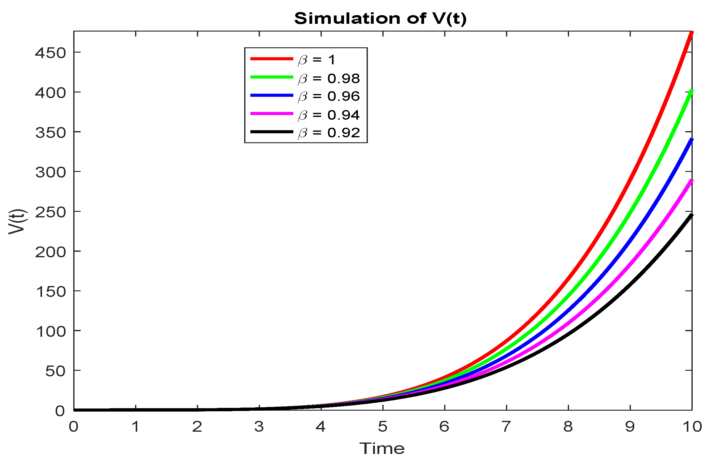
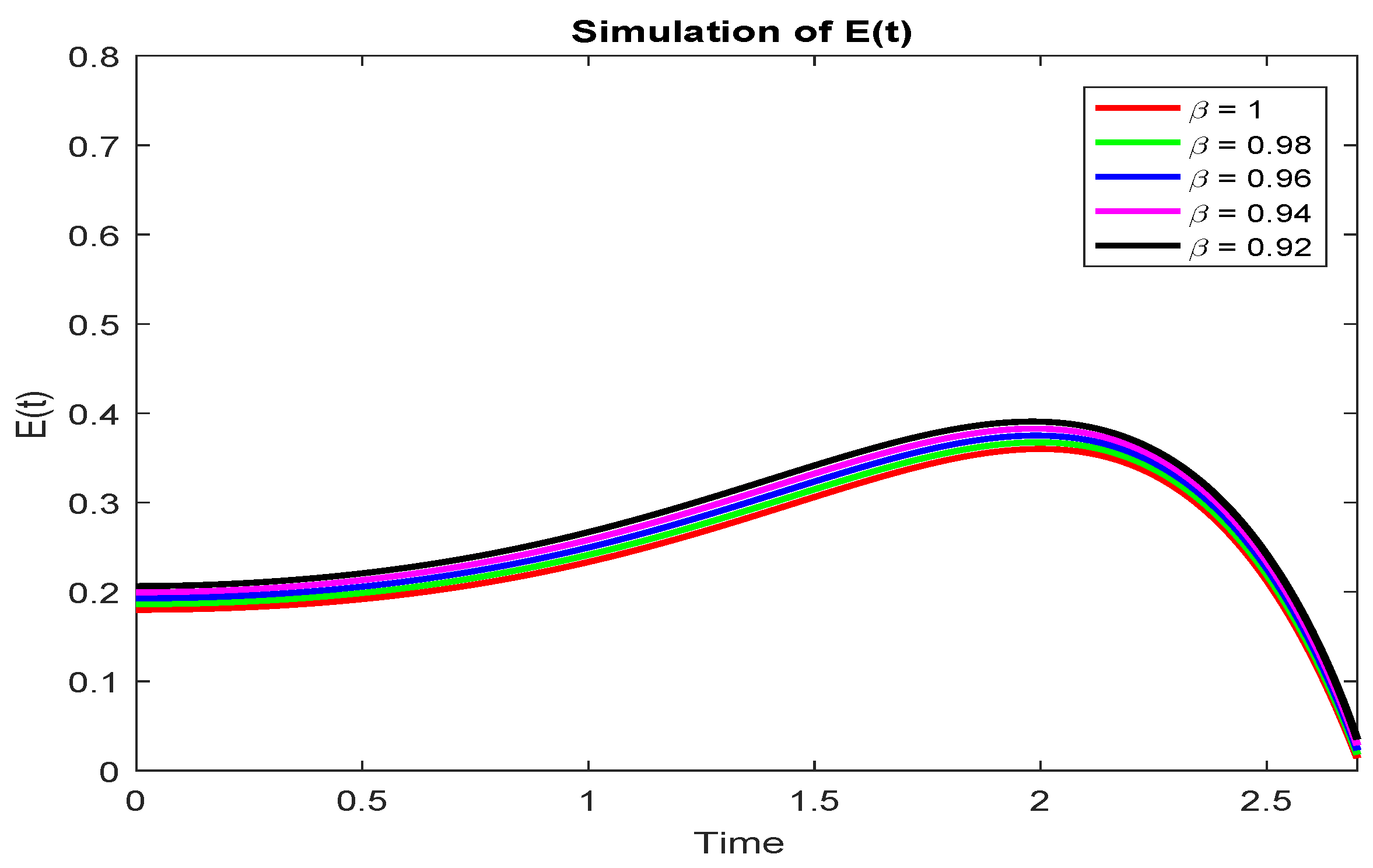
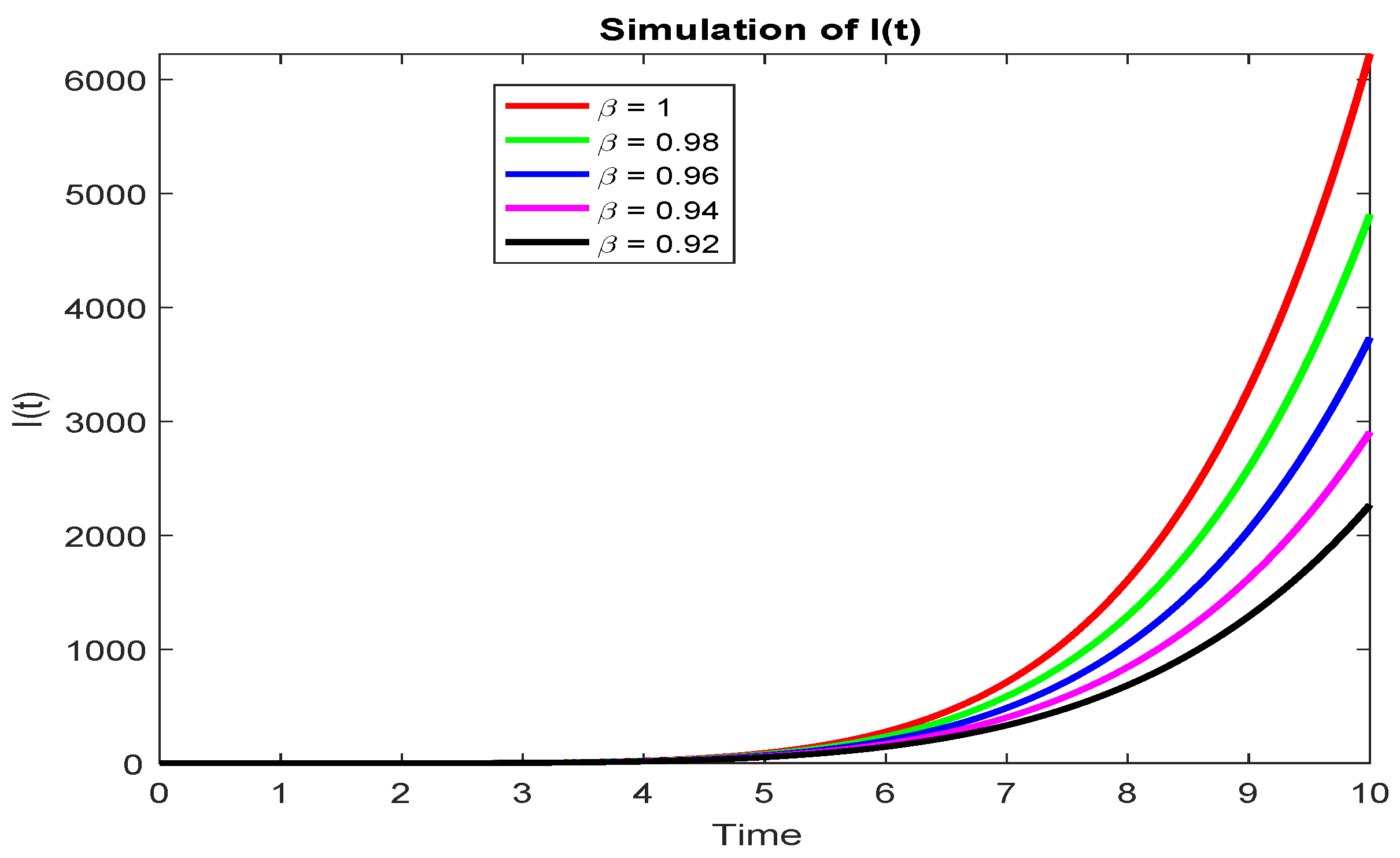
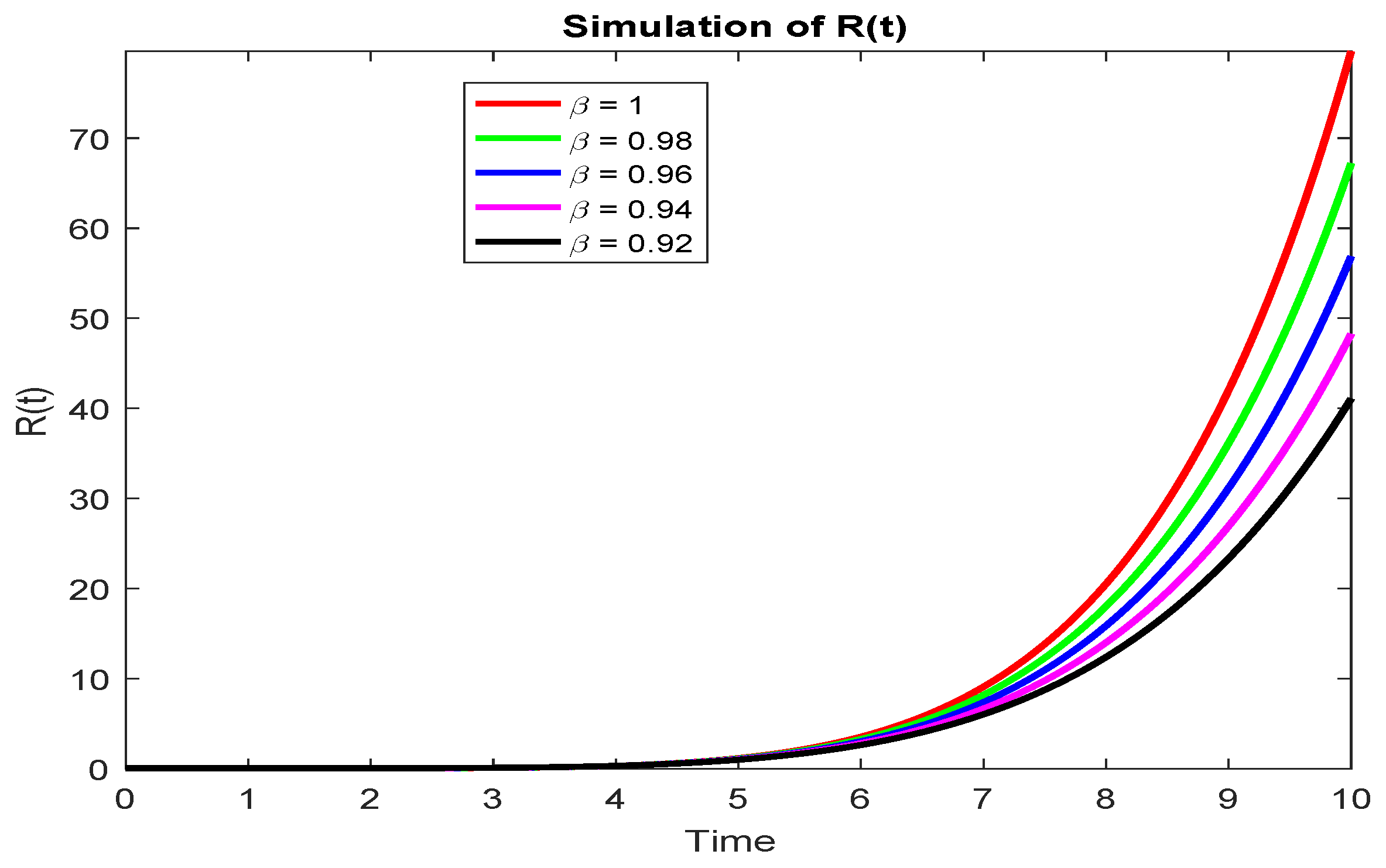
6. Result and Discussion

In this section, a simulation of considered model is illustrated in the figures using the value of the basic parameters from [10], which are $\varphi$ = 68,027, $\mu =0.000309$, $\delta =0.3720$, $\pi =0.000001$, $\omega =0.003286$, $\alpha =1\times {10}^{-9}$, $\beta =0.500000$, $\rho =0.036246$, and $\sigma =0.062366$ for reproduction number $R_0>1$. We have used initial values ${\mathcal{S}}_0=0.440$, ${\mathcal{V}}_0=0.230$, ${\mathcal{E}}_0=0.180$, ${\mathcal{I}}_0=0.070$, ${\mathcal{H}}_0=0.050$, and ${\mathcal{R}}_0=0.030$ from [10] such that the total population is $\mathcal{N}=\mathcal{S}+\mathcal{V}+\mathcal{E}+\mathcal{I}+\mathcal{H}+\mathcal{R}=1$. Figure 1, Figure 2, Figure 3, Figure 4, Figure 5 and Figure 6 show the plots for the variations in $\mathcal{S}$, $\mathcal{V}$, $\mathcal{E}$, $\mathcal{I}$, $\mathcal{H}$, and $\mathcal{R}$, for reproductive number $D_{rep}>1$, using different fractional order $\gamma =0.98,0.96,0.94$, and $0.92.$ We plotted the series solutions given in Equation (74) corresponding to different fractional order in Figure 1, Figure 2, Figure 3, Figure 4, Figure 5 and Figure 6 using Matlab. We observed that a low vaccination rate, $\pi$, and hospitalization rate, $\rho$, produced an endemic equilibrium and the number of infected persons grows rapidly, whereas raising these rates produces a disease-free equilibrium. We found that the fractional order SVEIHR measles model has more degrees of freedom as compared to ordinary derivatives. The compartments of the considered model exhibit noteworthy feedback when non-integer values of the fractional parameter are used, and at small fractional orders, growth or decay activity moves more quickly than at larger fractional orders. It has been demonstrated that the fractional order derivatives, which are the most prominent and trustworthy element as compared to the classical order case, are more effective at explaining physical processes. Numerical results that have been provided depict the behaviours of the dynamics that can be found in the different fractional orders.

7. Conclusions

The control, planning, and reduction in the negative effects of infectious diseases in society in previous decades are key functions of mathematical modelling. In contrast to the classical model, the results of the fractional order model have a memory effect on the epidemic model. The proposed scheme’s qualitative and quantitative analyses are also covered. We also looked at local and global stability using the Lyapunov function. We employed various methods to invert the PC and CPC operators in order to assess the fractional integral operator. We also derived the eigenfunctions of the CPC operator from the fractional differential equations of our proposed model. Additional analysis on the CPC and Hilfer generalised proportional operators is covered in great detail. A numerical simulation of a system of fractional differential equations is created employing the LADM. To simulate the outcomes for different fractional orders and fractal dimension values, we used Matlab. We have observed that the considered operator produces excellent results when applied to the mathematical modelling of a measles epidemic model. The figures demonstrate that changing the fractal order affects the behaviour of the measles model. Fractional order derivatives aid in the analysis of infection behaviour from beginning to end. The diagrams demonstrate the interactions between fractals and fractional orders. The graphical results lead us to the conclusion that the proposed model can be successfully used as a modelling tool and provides further insights into the dynamics of infectious diseases such as measles.

References

1. Griffin, D.E. The immune response in measles: Virus control, clearance and protective immunity. Viruses 2016, 8, 282. [Google Scholar] [CrossRef] [PubMed]
2. Subaiya, S.; Tabu, C.; Nganga, J.; Awes, A.A.; Sergon, K.; Cosmas, L.; Styczynski, A.; Thuo, S.; Lebo, E.; Kaiser, R.; et al. Use of the revised World Health Organization cluster survey methodology to classify measles-rubella vaccination campaign coverage in 47 counties in Kenya, 2016. PLoS ONE 2018, 13, e0199786. [Google Scholar] [CrossRef] [PubMed]
3. Guideline on Measles Surveillance and Outbreak Management. Available online: https://www.ephi.gov.et/images/guidelines/guideline-on-measles-surveillance-and-outbreak-management2012.pdf (accessed on 2 December 2022).
4. Measles, Preprint 2018. Measles. Available online: https://www.who.int/news-room/fact-sheets/detail/measles (accessed on 2 December 2022).
5. Farman, M.; Akgl, A.; Ahmad, A.; Baleanu, D.; Umer Saleem, M. Dynamical transmission of coronavirus model with analysis and simulation. Comput. Model. Eng. Sci. 2021, 127, 753–769. [Google Scholar] [CrossRef]
6. El Hajji, M.; Albargi, A.H. A mathematical investigation of an SVEIR epidemic model for the measles transmission. Math. Biosc. Eng. 2022, 19, 2853–2875. [Google Scholar] [CrossRef] [PubMed]
7. Tabassum, M.F.; Akgul, A.; Akram, S.; Farman, M.; Karim, R.; Hassan, S.M.U. Treatment of dynamical nonlinear Measles model: An evolutionary approach. Int. J. Nonlinear Anal. Appl. 2022, 13, 1629–1638. [Google Scholar]
8. Mitku, S.N.; Koya, P.R. Mathematical modeling and simulation study for the control and transmission dynamics of measles. Am. J. Appl. Math. 2017, 5, 99–107. [Google Scholar] [CrossRef]
9. Paul, R.V.; Atokolo, W.; Saka, S.A.; Joseph, A.O. Modeling the Transmission Dynamics of Measles in the Presence of Treatment as Control Strategy. Math. Sci. 2021, 17, 76–86. [Google Scholar] [CrossRef]
10. James Peter, O.; Ojo, M.M.; Viriyapong, R.; Abiodun Oguntolu, F. Mathematical model of measles transmission dynamics using real data from Nigeria. J. Differ. Equ. Appl. 2022, 28, 753–770. [Google Scholar] [CrossRef]
11. Farooq, M.M.; Mohsin, M.; Farman, M.; Akgl, A.; Saleem, M.U. Generalization method of generating the continuous nested distributions. Int. J. Nonlinear Sci. Numer. Simul. 2022. epub ahead of print. [Google Scholar] [CrossRef]
12. Xu, C.; Farman, M.; Akgl, A.; Nisar, K.S.; Ahmad, A. Modeling and analysis fractal order cancer model with effects of chemotherapy. Chaos Solitons Fractals 2022, 161, 112325. [Google Scholar] [CrossRef]
13. Farman, M.; Aslam, M.; Akgl, A.; Jarad, F. On Solutions of the Stiff Differential Equations in Chemistry Kinetics with Fractal-Fractional Derivatives. J. Comput. Nonlinear Dyn. 2022, 17, 071007. [Google Scholar] [CrossRef]
14. Farman, M.; Akgl, A.; Ahmad, A.; Saleem, M.U.; Ahmad, M.O. Modeling and analysis of computer virus fractional order model. In Methods of Mathematical Modelling; Academic Press: Cambridge, MA, USA, 2022; pp. 137–157. [Google Scholar]
15. Doungmo Goufo, E.F.; Oukouomi Noutchie, S.C.; Mugisha, S. A fractional SEIR epidemic model for spatial and temporal spread of measles in metapopulations. Abstr. Appl. Anal. 2014, 2014, 781028. [Google Scholar]
16. Nazir, G.; Shah, K.; Alrabaiah, H.; Khalil, H.; Khan, R.A. Fractional dynamical analysis of measles spread model under vaccination corresponding to nonsingular fractional order derivative. Adv. Differ. Equ. 2020, 2020, 171. [Google Scholar] [CrossRef]
17. Farman, M.; Saleem, M.U.; Ahmad, A.; Ahmad, M.O. Analysis and numerical solution of SEIR epidemic model of measles with non-integer time fractional derivatives by using Laplace Adomian Decomposition Method. Ain Shams Eng. J. 2018, 9, 3391–3397. [Google Scholar] [CrossRef]
18. Ogunmiloro, O.M.; Idowu, A.S.; Ogunlade, T.O.; Akindutire, R.O. On the Mathematical Modeling of Measles Disease Dynamics with Encephalitis and Relapse Under the Atangana Baleanu Caputo Fractional Operator and Real Measles Data of Nigeria. Int. J. Appl. Comput. Math. 2021, 7, 1–20. [Google Scholar] [CrossRef]
19. Qureshi, S. Real life application of Caputo fractional derivative for measles epidemiological autonomous dynamical system. Chaos Solitons Fractals 2020, 134, 109744. [Google Scholar] [CrossRef]
20. Abboubakar, H.; Fandio, R.; Sofack, B.S.; Ekobena Fouda, H.P. Fractional dynamics of a measles epidemic model. Axioms 2022, 11, 363. [Google Scholar] [CrossRef]
21. Qureshi, S. Monotonically decreasing behavior of measles epidemic well captured by Atangana Baleanu Caputo fractional operator under real measles data of Pakistan. Chaos Solitons Fractals 2020, 131, 109478. [Google Scholar] [CrossRef]
22. Nuwahereze, D.; Onuorah, M.O.; Abdulahi, B.M.; Kabandana, I. Standard Incidence Model of Measles with two Vaccination Strategies. World Sci. News 2022, 170, 149–171. [Google Scholar]
23. Kumar, S.; Kumar, R.; Osman, M.S.; Samet, B. A wavelet based numerical scheme for fractional order SEIR epidemic of measles by using Genocchi polynomials. Numer. Methods Partial. Differ. Equ. 2021, 37, 1250–1268. [Google Scholar] [CrossRef]
24. Farman, M.; Akgl, A.; Tekin, M.T.; Akram, M.M.; Ahmad, A.; Mahmoud, E.E.; Yahia, I.S. Fractal fractional-order derivative for HIV/AIDS model with Mittag–Leffler kernel. Alex. Eng. J. 2022, 61, 10965–10980. [Google Scholar] [CrossRef]
25. Yang, X.; Su, Y.; Yang, L.; Zhuo, X. Global analysis and simulation of a fractional order HBV immune model. Chaos Solitons Fractals 2022, 154, 111648. [Google Scholar] [CrossRef]
26. Baleanu, D.; Ghassabzade, F.A.; Nieto, J.J.; Jajarmi, A. On a new and generalized fractional model for a real cholera outbreak. Alex. Eng. J. 2022, 61, 9175–9186. [Google Scholar] [CrossRef]
27. Farman, M.; Amin, M.; Akgl, A.; Ahmad, A.; Riaz, M.B.; Ahmad, S. Fractal fractional operator for COVID-19 (Omicron) variant outbreak with analysis and modeling. Results Phys. 2022, 39, 105630. [Google Scholar] [CrossRef] [PubMed]
28. Eskandari, Z.; Avazzadeh, Z.; Khoshsiar Ghaziani, R.; Li, B. Dynamics and bifurcations of a discrete-time Lotka Volterra model using nonstandard finite difference discretization method. Math. Methods Appl. Sci. 2022. early view. [Google Scholar] [CrossRef]
29. Xu, C.; ur Rahman, M.; Baleanu, D. On fractional-order symmetric oscillator with offset-boosting control. Nonlinear Anal. Model. Control 2022, 27, 994–1008. [Google Scholar] [CrossRef]
30. Trigeassou, J.C.; Maamri, N.; Sabatier, J.; Oustaloup, A. A Lyapunov approach to the stability of fractional differential equations. Signal Process. 2011, 91, 437–445. [Google Scholar] [CrossRef]
31. Xu, C.; Farman, M.; Hasan, A.; Akgl, A.; Zakarya, M.; Albalawi, W.; Park, C. Lyapunov Stability and Wave Analysis of COVID-19 Omicron Variant of Real Data with Fractional Operator. Alex. Eng. J. 2022, 61, 11787–11802. [Google Scholar] [CrossRef]
32. Almeida, R.; Agarwal, R.P.; Hristova, S.; O’Regan, D. Quadratic Lyapunov Functions for Stability of the Generalized Proportional Fractional Differential Equations with Applications to Neural Networks. Axioms 2021, 10, 322. [Google Scholar] [CrossRef]
33. Saleem, M.U.; Farman, M.; Ahmad, A.; Ehasan, H.; Ahmad, M.O. A Caputo Fabrizio Fractional Order Model for Control of Glucose in Insulin Therapies for Diabetes. Ain Shams Eng. J. 2018, 11, 1309–1316. [Google Scholar] [CrossRef]
34. Ali, A.; Erturk, V.S.; Zeb, A.; Khan, R.A. Numerical solution of fractional order immunology and aids model via Laplace transform Adomian decomposition method. J. Fract. Calcul. Appl. 2019, 10, 242–252. [Google Scholar]
35. Baleanu, D.; Aydogn, S.M.; Mohammadi, H.; Rezapour, S. On modelling of epidemic childhood diseases with the Caputo-Fabrizio derivative by using the Laplace Adomian decomposition method. Alex. Eng. J. 2020, 59, 3029–3039. [Google Scholar] [CrossRef]
36. Sweilam, N.H.; Al-Mekhlafi, S.M.; Baleanu, D. A hybrid fractional optimal control for a novel Coronavirus (2019-nCov) mathematical model. J. Adv. Res. 2021, 32, 149–160. [Google Scholar] [CrossRef]
37. Gnerhan, H.; Dutta, H.; Dokuyucu, M.A.; Adel, W. Analysis of a fractional HIV model with Caputo and constant proportional Caputo operators. Chaos Solitons Fractals 2020, 139, 110053. [Google Scholar] [CrossRef]
38. Baleanu, D.; Fernandez, A.; Akgl, A. On a fractional operator combining proportional and classical differintegrals. Mathematics 2020, 8, 360. [Google Scholar] [CrossRef]
39. Anderson, D.R.; Ulness, D.J. Newly defined conformable derivatives. Adv. Dyn. Syst. Appl. 2015, 10, 109–137. [Google Scholar]
40. Van den Driessche, P.; Watmough, J. Reproduction numbers and sub-threshold endemic equilibria for compartmental models of disease transmission. Math. Biosci. 2002, 180, 29–48. [Google Scholar] [CrossRef]
41. Ahmed, I.; Kumam, P.; Jarad, F.; Borisut, P.; Jirakitpuwapat, W. On Hilfer generalized proportional fractional derivative. Adv. Differ. Equ. 2020, 2020, 329. [Google Scholar] [CrossRef]
Figure 1. Simulation of S ( t ) proposed fractional operator.
Symmetry 15 00468 g001
Figure 2. Simulation of V ( t ) proposed fractional operator.
Symmetry 15 00468 g002
Figure 3. Simulation of E ( t ) proposed fractional operator.
Symmetry 15 00468 g003
Figure 4. Simulation of I ( t ) proposed fractional operator.
Symmetry 15 00468 g004
Figure 5. Simulation of H ( t ) proposed fractional operator.
Symmetry 15 00468 g005
Figure 6. Simulation of R ( t ) proposed fractional operator.
Symmetry 15 00468 g006
Disclaimer/Publisher’s Note: The statements, opinions and data contained in all publications are solely those of the individual author(s) and contributor(s) and not of MDPI and/or the editor(s). MDPI and/or the editor(s) disclaim responsibility for any injury to people or property resulting from any ideas, methods, instructions or products referred to in the content.