
Study of Propeller Vortex Characteristics under Loading Conditions

1
State Key Laboratory of Structural Analysis for Industrial Equipment, Dalian University of Technology, Dalian 116000, China
2
Marine Engineering College, Dalian Maritime University, Dalian 116026, China
3
Internet of Things Thrust, The Hong Kong University of Science and Technology (Guangzhou), Nansha, Guangzhou 511400, China
*
Authors to whom correspondence should be addressed.
Symmetry 2023, 15(2), 445; https://doi.org/10.3390/sym15020445
Submission received: 9 January 2023
/
Revised: 28 January 2023
/
Accepted: 1 February 2023
/
Published: 7 February 2023
(This article belongs to the Special Issue Physics and Symmetry Section: Feature Papers 2022)
Abstract
:Marine load is an important factor affecting propeller propulsion efficiency, and the study of the wake evolution mechanism under different conditions is an essential part of the propeller equipment design, which needs to meet the requirements of complex engineering. Based on the large eddy simulation (LES) method, the wake instability characteristics are researched with the hydrodynamic load and wake dynamics theory, and the vortices composition and evolution mechanism under various load conditions are analyzed. Meanwhile, the propeller wake using the unsteady Reynolds-averaged Navier–Stokes (URANS) and LES methods is numerically simulated and compared. In addition, a comparison between a simulation and an experiment is carried out. The vortices evolution is described by dimensionless values of the velocity, pressure field, and vorticity field. The breaking and reassembling of different vortices are discussed. The results show that the pitch of the helicoidal tip vortices is larger under light loading conditions with high advance coefficients, and the wake is more stable, in contrast, which is smaller and the vortices break down earlier. By comparison, the topology of the vortices system is more complex under the low advance coefficient. Considering the interference effect between adjacent tip vortices, the energy dissipation is accelerated, resulting in the increased instability of vortices.
1. Introduction
The propeller is the most common power device in ships, and its performance has become a hot issue for researchers, including its hydrodynamic performance, cavitation performance, and noise performance. The subjects covered include improving energy-saving efficiency, reducing fuel consumption, and ensuring the economic benefits with safe operation, which is a major research area in the navigation field. A complex physical field is generated behind the propeller operating in the water, which is called the propeller wake. In the complex wake, the vortices evolve continuously, and their characteristics are closely related to ship performance, operation, etc. Therefore, the analysis of vortex evolution in the propeller wake can help to reduce the flow and vibration noise generated by the operation [1], and to realize a propeller energy-saving design, which is a long-standing requirement. In the pre-design stage, one of the most attractive and challenging topics is the evolution analysis of the propeller wake vortex in hydrodynamics, which is an important reference for improving ship performance.
Anirban et al. [2] conducted experiments on the characteristics of propeller propulsion under actual wave conditions and showed that the effect of the wake field is an important reason for the large differences in the efficiencies of different propellers. A comparative numerical analysis of the evolution of the wake vortex generated by the propeller during the test was carried out [3]. The detached eddy simulation (DES), a numerical simulation method, was used to comprehensively analyze the propeller composition, three-dimensional structure, wake vortex contraction, and evolution rules. The characteristics of the vortical structures of the ducted propeller model (DPM) wake were described by the method in detail. Thanks to the computational fluid dynamics (CFD) development in recent years, the characteristics of the wake field can be revealed by simulations, which is difficult in experiments. The RANS/LES method is increasingly used in the CFD simulation of propellers to realize the mutual complement of an open water test [4]. Dubbioso et al. [5] carried out numerical calculations of propellers to investigate their hydrodynamic characteristics under multiple load cases by using the RANS method. The influence of non-axisymmetric inflow conditions was studied for the non-uniform distribution of the load on the propeller plane surface. The causes of wake vortex interference and enhanced diffusion effects were also analyzed in the local area behind the propeller. Based on the LES method, Posa et al. [6] analyzed the characteristics of wake vortex evolution and the interference effect between the hub vortex and hydrofoil boundary layer. Wang et al. [7] showed that the interaction between the tip vortex and the secondary tip vortex at the end plate was an important factor that triggered the leapfrog phenomenon and induced external instability. When the internal tail vortex or root vortex is coherent, it will experience contraction and approach the hub vortex and then intertwine with it to form the dominant mode of the propeller wake.
Hu et al. [8] investigated the evolution of the propeller tip vortex and its effect on the rudder surface pressure fluctuation using a large eddy simulation. They showed that the propeller tip vortex became dislocated and shrank owing to its interactions with the propeller by studying the relationship between the vortex flow field and the advance ratio. The effect of the blade tip vortex leads to a strong periodicity of the rudder surface pressure, while that within the hub vortex is relatively random. Magionesi et al. [9] showed a dependence of the spatial shape of the modes and the temporal scales on the evolution and destabilization mechanisms of the wake past the propeller. The phenomenon of destabilization of the wake, originated by the coupling of consecutive tip vortices, and the mechanisms of hub–tip vortex interaction and wake meandering are identified by both proper orthogonal decomposition (POD) and dynamic mode decomposition (DMD).
Felli et al. [10] investigated experimentally the mechanisms of the evolution of the propeller tip and hub vortices in the transitional region and the far-field region and examined the effect of the spiral-to-spiral distance on the mechanisms of wake evolution and instability transition. The study showed the relationship of the wake instability with the spiral-to-spiral distance and a multistep grouping mechanism among the tip vortices.
The study in this paper focuses on a non-sloping uniform inlet propeller wake flow field with a symmetric flow field. From the related literature, the loading condition has a significant effect on the propeller propulsion efficiency, especially for maritime vessels. Considering the loading effect on the instability of the propeller wake, taking the MAU propeller as the object, numerical simulations of its wake field are carried out, and the wake evolution processes under different loading conditions are obtained, which provide a reference for the design of a high-efficiency propeller for complex engineering.
2. Mathematical Models
2.1. Unsteady Reynolds-Averaged Navier–Stokes
The RANS method is now widely used in engineering practice by solving the time-averaged equation, which can make accurate forecasts while significantly reducing the computational cost. However, based on the RANS model, the flow conditions’ changes in time are ignored by the averaging operation, which cannot reflect the instantaneous characteristics of the flow field. The RANS model is based on a definition of a mean value with specific properties [11,12]. Considering the fluctuation influence, the turbulent motion using the time-averaged method is deemed as a sum of the time-averaged flow and the instantaneous fluctuation flow. In the RANS method, the time-averaged value is defined by the variable , as shown in Equation (1).
where is an instantaneous value that is equal to the sum of the time-averaged value and the fluctuation value .
Whenever the computed solution is time-dependent, a phase average can be introduced for unsteady flows with some fundamental frequencies, which has led to RANS modeling becoming commonly renamed as URANS. Applying the URANS model can resolve some of the unsteady features of the flow without the recalibration of model coefficients. The use of the URANS method is advocated in cases of clear scale separation, and URANS simulations can be substantially more successful than a steady RANS computation, especially in determining the mean flow [13]. The connection between the time-averaged and fluctuation values is established using the RANS method through a turbulence model. In the viscous vortex model, the turbulent viscosity is represented by the turbulent stress . The k-ω model is a two-equations model, as shown in Equations (2) and (3), which is composed of the fluctuation transport equations of turbulent kinetic energy k and specific turbulent dissipation rate ω. The shear stress transport (SST) k-ω model [14,15] is more efficient in forecasting shear flow and has good adaptability to both near-wall and far-field regions. Meanwhile, the model has higher computational accuracy and reliability, and, especially, a significant advantage in rotating flow.
where is the fluid density; is time; is the velocity, are the components of x, y, and z directions, respectively; is the correlation term of the laminar velocity gradient; is the gradient correlation term corrected for the Reynolds number in ; are the turbulence caused by diffusion; is the diffusivity of k; is the diffusivity of; is the orthogonal divergence term introduced by the SST k-ω model, as shown in Equation (4); is the model mixing function; is turbulent kinetic energy; is specific dissipation rate; is a custom turbulent dissipation-related term; and = 0.856; refer to the article of Zhang et al. [16] for more details about the turbulence model.
2.2. Spectral Fatigue Analysis Method
The non-linear convection term in the transport equation introduces an unclosed term, describing the impact of the sub-filter scales on the resolved motion. As for RANS modeling, it is replaced by a model term , which is usually called the subgrid-scale (SGS) model. LES is often introduced based on the filtering concept [17], and the filter width is the key parameter of the model, usually called . The step size of the grid determines the corresponding parameters in the model by affecting the cutoff scale of the filter. can maximize the benefit from the resolution capacity of the grid in shifting the cutoff of the implicitly introduced filter to higher wavenumbers through the grid being refined. The ratio of to is usually set to 1 to improve computational efficiency.
LES solves large-scale turbulence and models small-scale motion in the flow domain by directly simulating large-scale vortices and simplifying small-scale vortexes. Because it is very difficult to describe the structure of large vortices with different boundary characteristics using turbulence models, the LES method conducts a direct simulation of the turbulence fluctuation part by removing small-scale vortices through filtering in a small spatial range and then building a model to simulate the effect of small vortexes on large vortexes. The large-scale motion determines the turbulent kinetic energy K in the flow, and the dissipation rate ε is determined by the small scale [18], and then K is decomposed and ε simulated using the LES method. The LES method is popular for transient numerical simulation of the flow field, but it requires a high-performance computer.
The theoretical formula of the wall-adapting local eddy-viscosity (WALE) model adopts the form of a velocity gradient tensor. Although the model has some limitations in the model coefficient term, it is less sensitive to the value of the coefficient than the other SGS model. The model does not require near-wall damping and can automatically provide accurate wall scaling. Moreover, the effectiveness of the WALE SGS model applied in rotating machinery has been verified.
3. Numerical Set-Up
In engineering, generally, selecting propellers is based on the characteristics and technical requirements of ships. The propellers with higher adaptability to ships are selected by comparing the propellers that have different performances. In this paper, the MAU propeller is selected as the object, which is a propeller series mainly developed by the Japanese. It improves the cut shape, expands the range of disc and pitch ratio, and carries out a 3~6-blade propeller model test, then completes the design chart of the propeller.
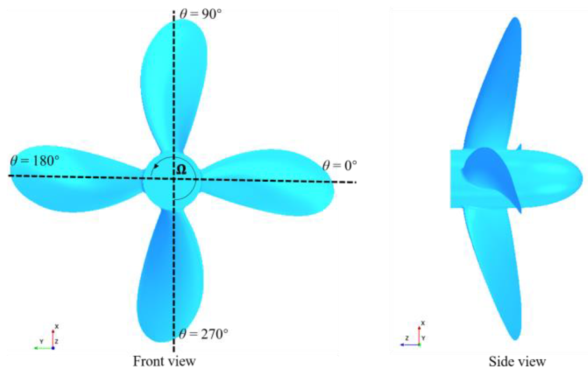
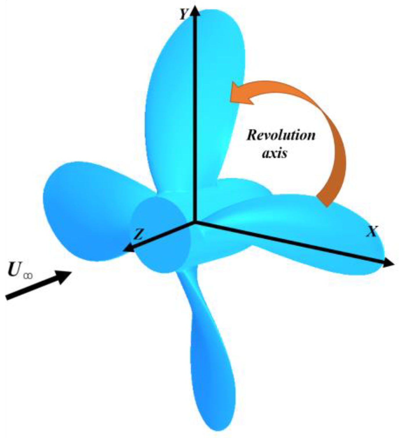
Considering the repeatability of numerical analysis, the MAU4-40 equal-pitch propeller is selected as the geometry reference for modeling in the study, as seen in Figure 1, and the main parameters of the propeller are seen in Table 1. The model reference coordinate system is O-XYZ, as seen in Figure 2. The origin O is located at the center of the rotation of the propeller; the Z-axis is along the direction of fluid flow; the Y-axis is perpendicular to the center of the propeller hub upward; and the X-axis can be determined according to the right-hand rule (r.h.s.). The numerical simulations in the paper were carried out for two operating conditions, respectively, such as the advance coefficient J = 0.3 and J = 0.6. The advance coefficient J is obtained by varying the incoming flow velocity U (inlet velocity) at a fixed speed n (n = 7.5 rps). Unless otherwise stated, all physical quantities were non-dimensionalized using characteristic parameters. Among them, the propeller radius (d = 0.125 m) was chosen as the characteristic length, the fluid density (ρ = 997.561 kg/m3) as the characteristic density, and the fixed rotational speed n (n = 7.5 rps). Re = (nD2)/ν = 5.27 × 10⁵, where is the kinematic viscosity.
The computational domain and boundary conditions of the simulation are presented in Figure 3. The computational domain consists of two cylinders along the flow direction containing the propeller. The propeller diameter (radius) D(d) is 0.25 (0.125) m, and the flow field area diameter is 9.6 D in a large cylinder, which is a size that better avoids the blocking effect on the propeller wake development. The inlet of the boundary condition is set as the velocity inlet to provide a uniform inflow, and the outlet condition is defined as the pressure outlet [19]. Considering the computational resources, the upstream velocity inlet of the boundary conditions in this paper is 4.8 D from the propeller, and the downstream pressure outlet is 9.6 D from the propeller. According to Kumar and Mahesh (2017), the size effect of the computational domain on the evolution of the propeller wake is negligible.
According to the characteristics of the turbulence model, in order to improve the computational efficiency, the boundary layer grid is tried as follows: the grid with y+ < 1 has a high accuracy, and the final grid number is 3.8 M, and the details of boundary layer grid test are seen in Table 2.
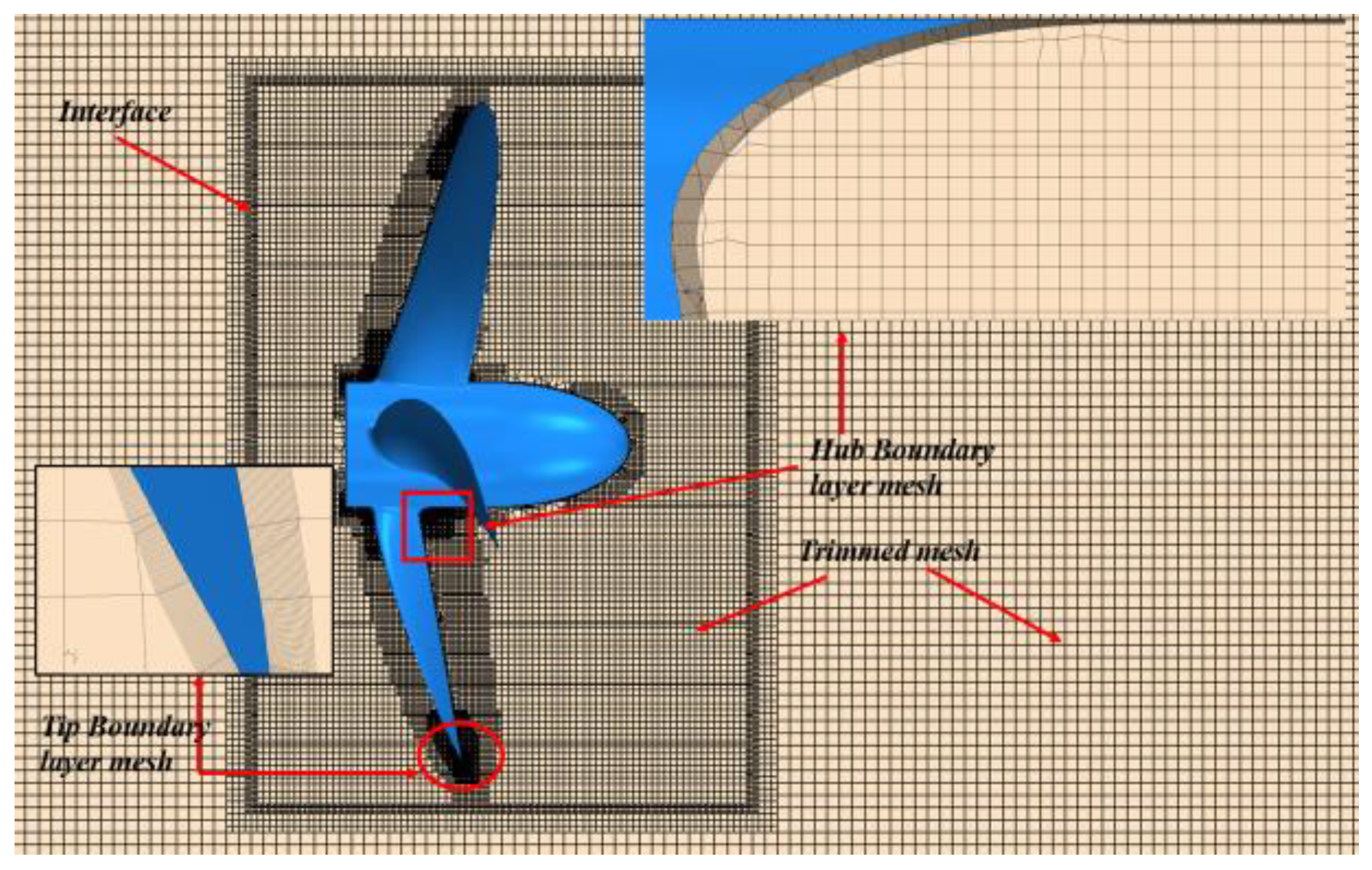
To meet the algorithm accuracy requirements and better capture the viscous flow in the near-wall boundary layer, the constraint y+ < 1 is set, and a boundary layer mesh containing 20 prismatic layers is used. To avoid the numerical dissipation of the system, multiple isotropic volumes (cylinders) with different dimensions are used to capture the fundamental flow features in the critical region. The specific settings are as follows: the blade tip region (1% D), the paddle hub region (2% D), and the dynamic domain region (3% D), and four encrypted regions are set as 8% D, 15% D, 20% D, and 30% D. Thus, it can capture enough tail flow details but saving computational resources as much as possible. The specific details of grid division are referred to in Figure 4. The sliding grid technique is used to divide the computational domain into static and rotating domains, based on which the data interaction between the interfaces is carried out. The contact surface between the static and rotating domains is set as the interface to realize the information exchange and iteration between the two domains. For slip boundary, the velocity of the fluid in the boundary method direction is 0, and the tangential velocity of the boundary is the component of the fluid in the velocity in the tangential direction. At the inflow, the velocity is set to the undisturbed flow value, that is, u = U, while at the outflow, the velocity is extrapolated from the interior point. Among them, the number of the coarse mesh is divided into 3.8 M for the MAU4-40 propeller open water working condition. The output thrust and torque magnitude of the propeller are reflected by by following Equations (5) and (6). is usually taken as 10 times the value of the parameter. is a dimensionless value defined based on the above parameter by following Equation (7), which is an important evaluation index of propeller propulsion efficiency.
where U is the incoming flow velocity; n is the rotational speed; ρ is the fluid density; and T is the output thrust and also the output torque.
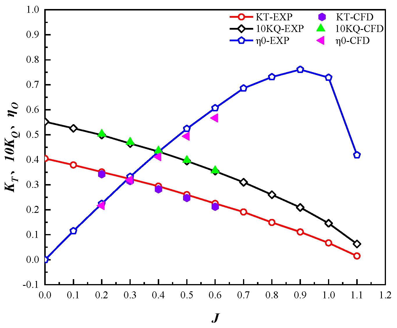
To verify the accuracy of the numerical calculation results in this paper, the CFD calculated values of the propeller performance curves (KT, 10 KQ, η) were compared with the test values. From Figure 5, the performance of the propeller calculated by the mesh system and numerical model matches well with the experimental results in the literature [20], and the average error of the calculated values (KT, 10 KQ, η) is less than 5%, which meets the engineering requirements. In summary, the numerical method and mesh system in this paper are suitable for analyzing the propeller wake characteristics. To improve the numerical accuracy of the wake field simulation, the dual mesh evaluation procedure proposed in the literature is adopted in this paper to perform mesh sensitivity analysis [21]. The dual mesh numbers are 18.94 M for the fine mesh number and 10.90 M for the medium mesh number. The refinement ratio of the mesh, the error estimate for the fine mesh, and the uncertainty are evaluated by the following equation.
where N denotes the total number of cells in the mesh, m denotes the dimensionality of the problem, and this paper is a three-dimensional problem, so m = 3 and ≈1.2; f1 and f2 correspond to the results of the fine and medium mesh, p is the formal order of accuracy (p = 2); FS is a safety factor assumed to be 3.
As shown in the table, the numerical results obtained using medium and fine meshing are very close, with not exceeding 2% in both cases, as seen in Table 3, indicating that the obtained solutions are relatively grid independent. Therefore, both the numerical solver and the grid strategy employed can be regarded as consistent and reliable. From the point of view of improving accuracy, the fine mesh is more suitable for practical applications. All subsequent analyses in the study were obtained from the fine mesh simulations.
The three-dimensional viscous flow field was solved by the finite volume method based on the discrete flow solver in the STAR-CCM+ computational fluid dynamics program, and the solution was stopped after the flow field was stable for 9 S. The turbulence model should be selected according to whether the fluid is compressible, the establishment of special feasible problems, accuracy requirements, computer capabilities, time constraints, and other conditions. This requires an understanding of the scope and limits of application of different conditions to select an appropriate model. The SST model adopts the K-W model for the near-wall surface and the K-E model for the non-near-wall surface, which can better take the influence of wall shear into account. The SST turbulence model is recommended by many scholars, especially in the case of precise computing grid division, so the SST turbulence model is used in this RANS calculation. For more details and a complete description of RANS/LES, the reader is directed to Posa et al. (2020), Di Mascio et al. (2014), and Wang et al. (2022).
4. Numerical Validation
4.1. Propeller Characteristics
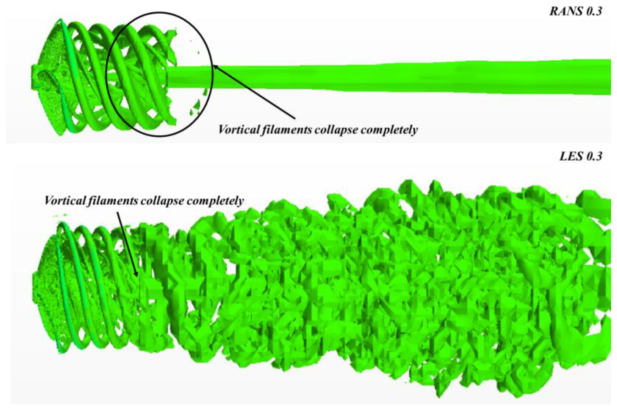
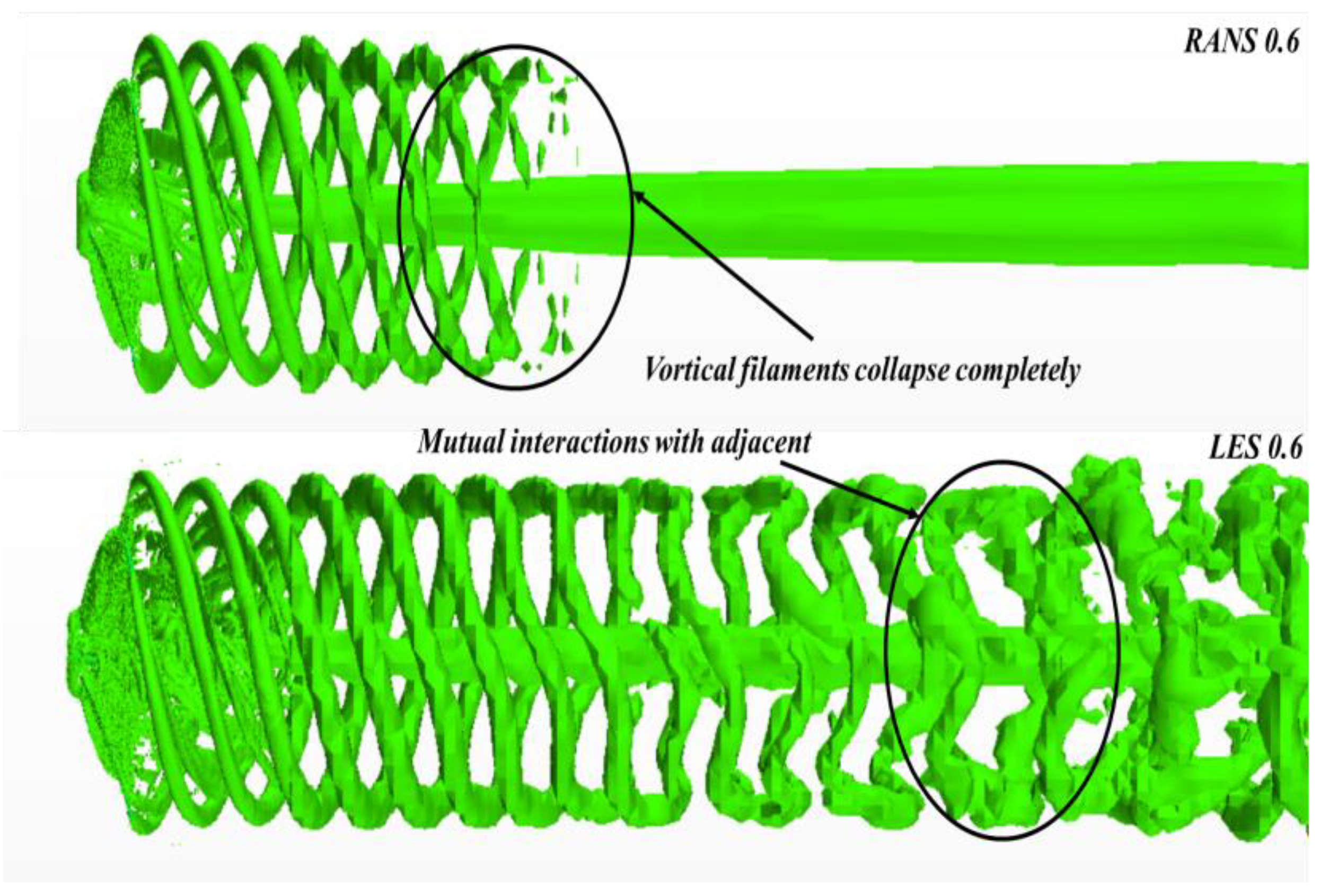
Figure 6 compares propeller wake vortical structures simulated by the LES using the iso-surfaces of the Q-criterion with vortical structures obtained from simulation using the URANS. These figures show that LES describes the evolution of the propeller wake far better, which is especially manifested in the process from instability to final breakdown. By contrast, the URANS could only make a limited capture aimed at some behavior.
Importantly, the wake vortical structures with three dimensions considering each of the two different advance coefficients captured by LES are remarkably similar to the ones with two dimensions. Due to the instantaneous visualizations, there are some slight differences in individual vortexes, which seems to be acceptable, as will be explained by showing the complete wake field in Section 5.
As observed in the subsequent wake field, the pitch of the tip vortex increases with the increase in the advance coefficient. Meanwhile, the propeller wake destabilizes and breaks down further downstream. Mainly, at the low advance coefficient (J = 0.3), it is observed that after the onset of the instabilities, the tip vortical structures collapse completely soon after. This is followed by the hub vortex breakup. Whereas, at the high advance coefficient (J = 0.6), the tip vortical structures break further downstream and experience mutual interactions with adjacent vortices before proceeding to complete collapse.
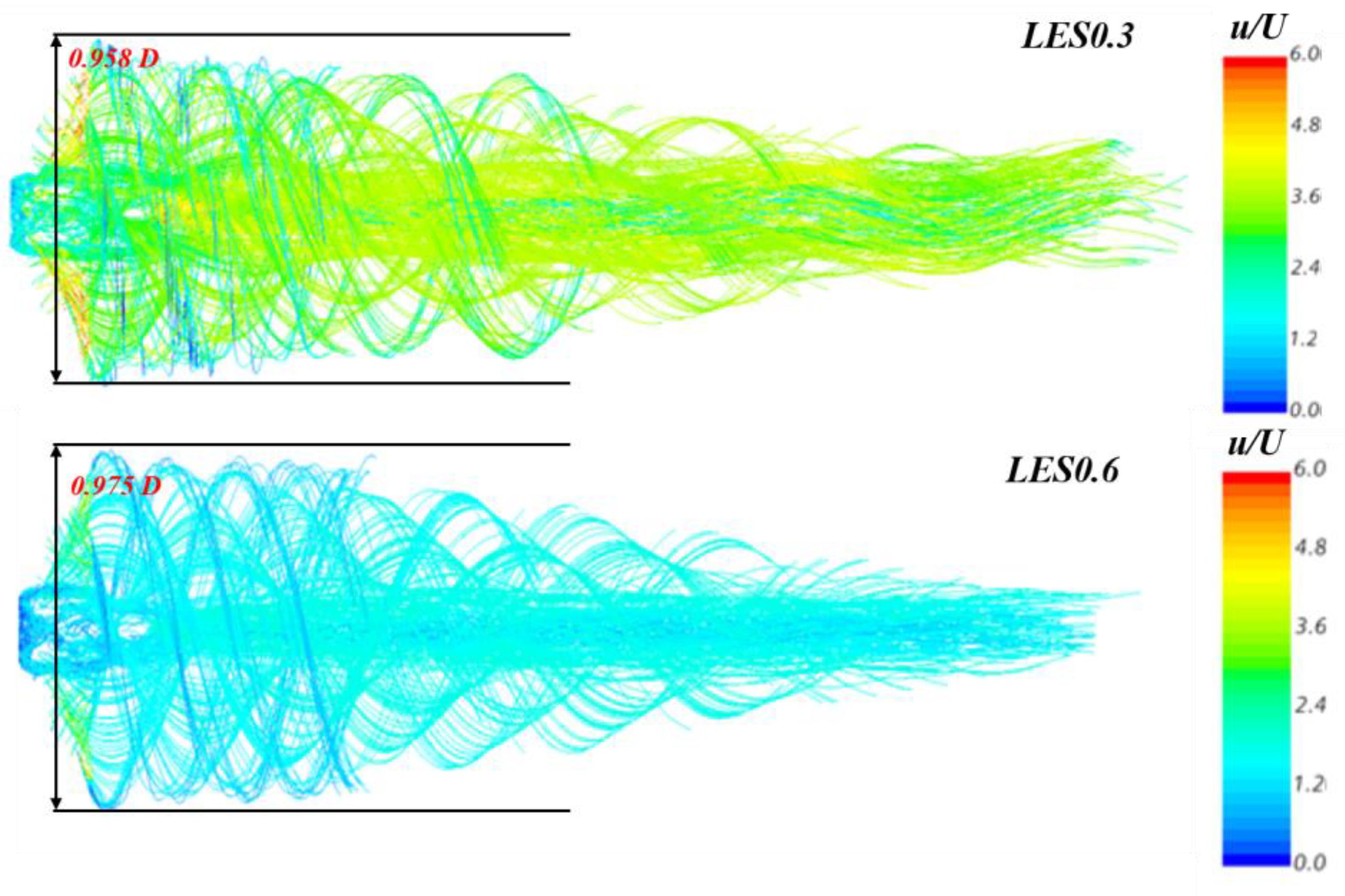
4.2. Streamlines
There are wake flow streamlines of the propeller under different load conditions as show in Figure 7. From the figures, when J = 0.3, the wake diameter is significantly smaller than the propeller, which is due to the strong suction role of the propeller on the fluid at low advanced coefficient. As J increases, the suction role decreases, and the wake diameter increases. Under the condition of J = 0.6, the suction role is not obvious, which can reduce energy loss and verifies the reason for high efficiency.
4.3. Pressure Coefficient (Cp) Contours on Propeller Blades
As shown in Figure 8, it can be seen that the pressure distribution on the pressure side decreases gradually along the rotation direction, and the maximum pressure is observed near the tip of the endplate. In addition, the pressure distribution on the suction side decreases suddenly in the initial phase and then gradually increases. The pressure core area is distributed radially in the band. Therefore, the pressure on the suction side is different from that on the pressure side; the air flow on the rear side first accelerates and then decelerates along the direction of rotation. It should be noted that for the suction side, the pressure gradient of the outer surface is greater than that of the inner surface, and the change in velocity is more unstable outside the inner surface of the suction side, which is more obvious in the results calculated by the LES method.
5. Instantaneous Characteristics Wake Field
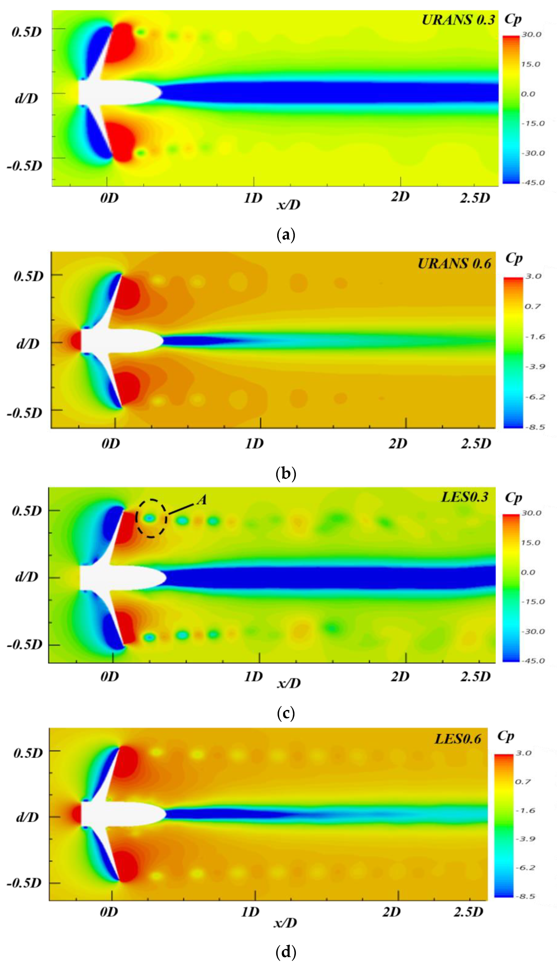
5.1. Instantaneous Cp Wake Field
Figure 9 shows the dimensionless pressure contour plot in the same plane. The pressure inside the vortex decreases as the blade load decreases, with the largest pressure drop occurring near the wake and inside the hub vortex. This pressure drop can lead to cavitation of the propeller blade, which can be severely damaged and lead to cavitation noise generation, and the cavitation generation should be delayed as much as possible in practical engineering. Compared to the URANS model, the LES shows a more pronounced negative pressure zone under a heavy load, position A, as shown in Figure 9.
As the load increases, both the negative pressure inside the vortex and the pressure variation in the near-paddle region increase, producing more adjacent high-pressure and low-pressure regions. This pressure variation is an important reason for the mutual interference of complex vortex system topologies under high-load operating conditions.
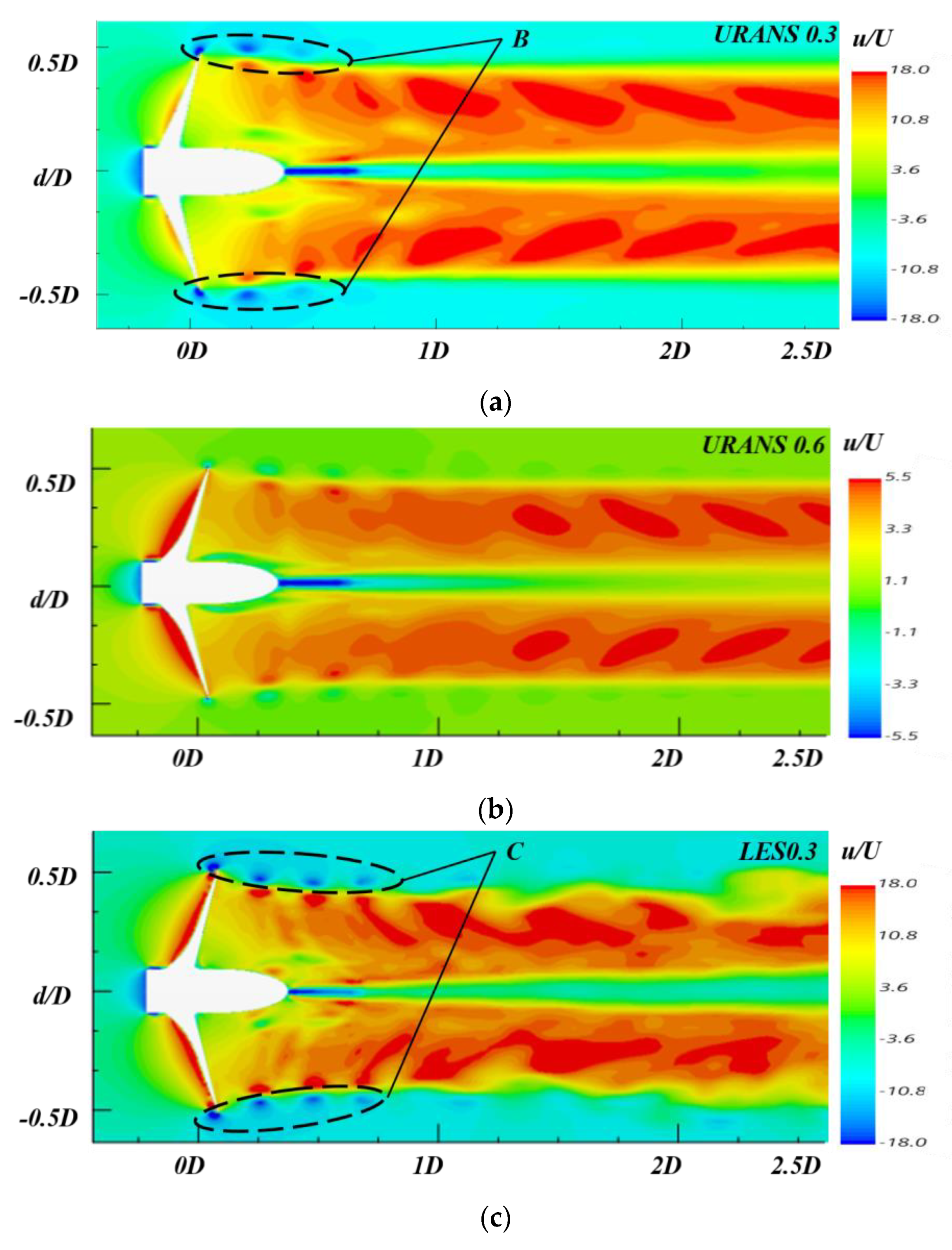
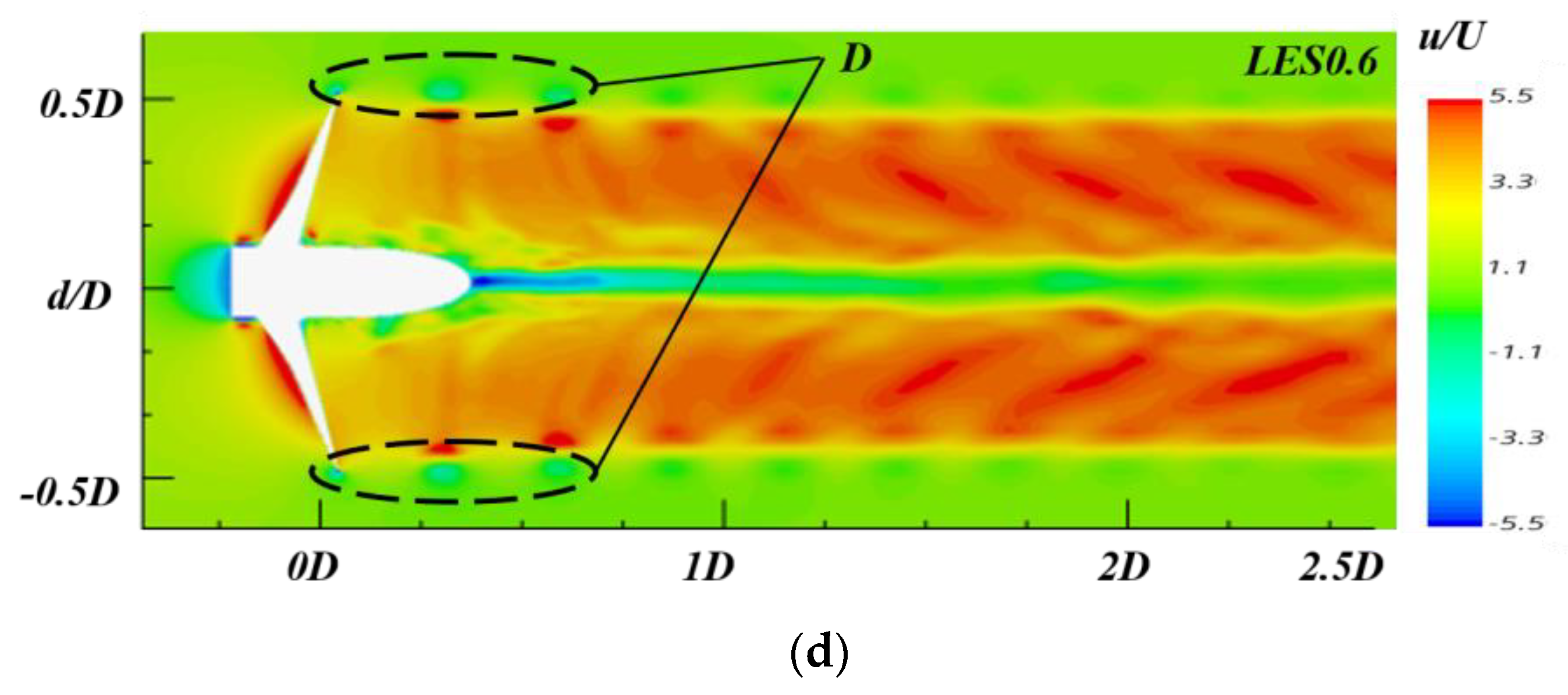
5.2. Instantaneous u/U Wake Field
Figure 10 shows the axial velocity. A comparison of different advance coefficients and different turbulence models is given, using the propeller advance velocity U for the dimensionless axial velocity. The dimensionless velocity field is axisymmetric under uniform inflow conditions. The velocity field behind the propeller is distributed with a “camel’s hump” velocity peak characteristic, which decreases and widens as the wake moves downstream due to the turbulent diffusion effect.
The effect of the boundary layer on the propeller blades is observed in this “low velocity region”. At the same time, as the water accelerates behind the propeller, these regions become more and more inclined as it progresses downstream. Further downstream, the effect of turbulent diffusion can be seen. Comparing the different turbulence models at the same dimensionless velocity, the LES model captures the “low velocity region” more clearly, located at Figure 10a B and Figure 7c C. When comparing the dimensionless velocities under different load conditions according to the LES calculation results, the velocity gradient in the blade tip vortex region and hub vortex region decreases as the load decreases, and the inclination of the “low speed “ is also smaller, as demonstrated at position C and D in Figure 10. Under heavy load conditions, the distance between the adjacent “low speed“ decreases, and the uneven velocity zone intensifies the interaction of the post-paddle vortex system structure and causes a larger energy loss, which is obtained by comparing the C and D areas in Figure 10.
In addition, the lowest negative velocities were observed at the beginning of the hub vortex, which is a near-hub flow suction phenomenon generated by the hub vortex. Negative velocities were also observed in a very small region of the first four blade tip vortices attached to the blades under heavy load conditions.
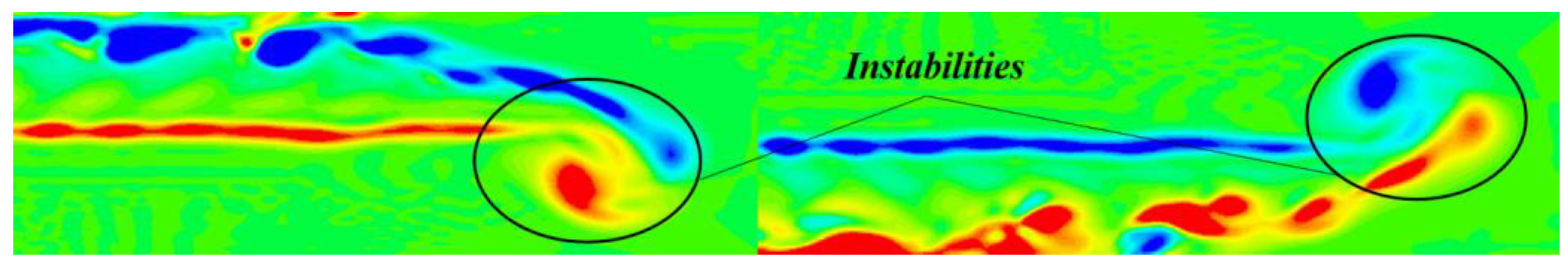
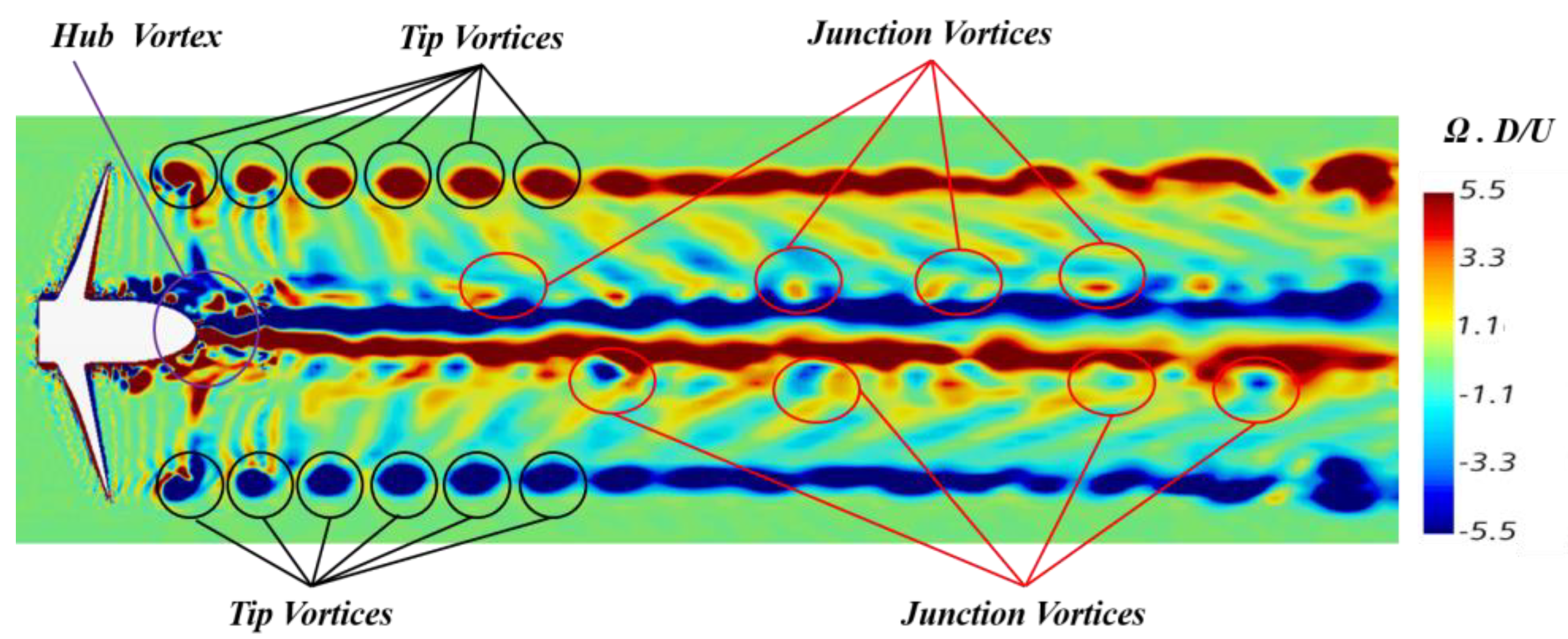
5.3. Vortical Structures
Figure 11 shows the state of the tail vortex field when the flow field is not stable. With the increase in the solution time, the flow field gradually stabilizes, and the final wake field is shown in Figure 12. Further capturing the variation in the vortex system caused by the propeller, Figure 12 presents a graphical analysis of the longitudinal vortex field in a typical motion moment and introduces the evolution of different vortices. A horseshoe-shaped vortex system spiral trajectory with opposite signs can be seen at the junction of the blade leading edge with the hub downstream to the convection (junction vortices) [22].
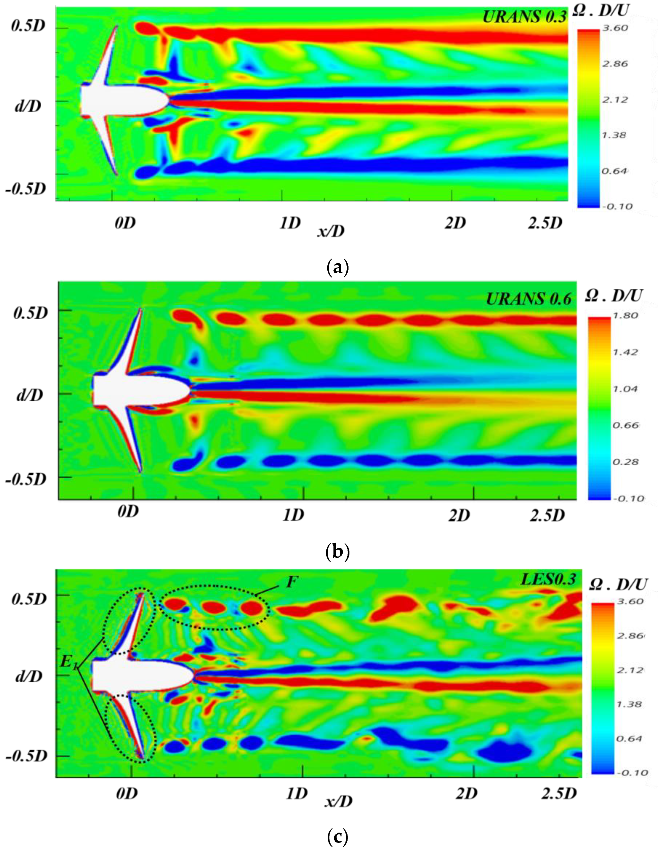
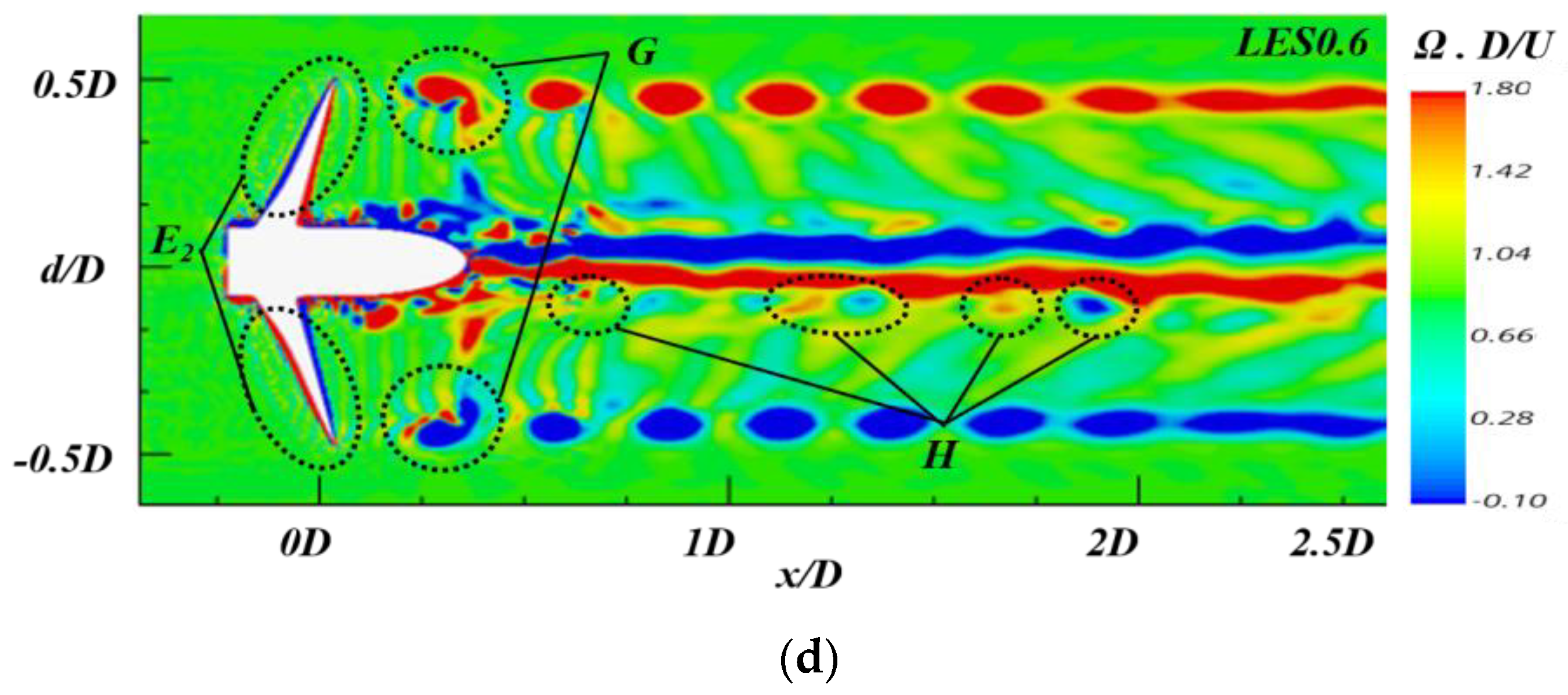
This coherent horseshoe-shaped vortex is important for identifying the mechanism leading to propeller wake instability. This phenomenon is more clearly observed at higher advance coefficients (J = 0.6), where the junction vortices start to break up into smaller vortex structures near the bottom (near the hub vortex) due to the greater intensity of the counter-rotating hub vortex than the blade tip vortex, leading to enhanced mutual interference between adjacent junction vortices and gradual destabilization of its propeller wake field (position H, Figure 13d).
On the other hand, the suction effect significantly alters the pressure and axial velocity distribution upstream of the propeller, manifesting firstly in the strong vortex system with opposite signs of shedding from the blade tip (i.e., tip vortex) and in the vortex system with an intense flow at the rear of the hub (i.e., hub vortex) seen on the leeward and windward sides of the wake field [22], where the hub vortex is formed by the merging of root vortices shedding from the blades and involves detachment from the hub of the shear layer. This is evident from the transient vortex fields in Figure 12.
Steep pressure gradients (Figure 9) near the propeller blade tip were captured for both loading conditions and both methods, a condition that keeps the vortices merged in the vortex region of the blade tip vortex stable. At the same time, the vortex attached to the propeller blade surface formed vortex structures that exhibited different morphologies on the leeward and windward side, evolving along the downstream direction with the tip vortices. The LES method in the near-wall region can accurately capture the “secondary tip vortices” in region G in Figure 13d. However, the URANS method is not able to capture this phenomenon. Under heavy load conditions, the strong vortices of opposite signs in the blade back part are mixed (Figure 13c E1 and Figure 13d E2). These opposite vortices interact and collide along the blade tip direction, making the topology of the vortex system more complex and leading to increased instability and gradual destabilization of the vortex structure.
The area where the hub vortex causes low pressure is susceptible to cavitation. The hub vortex undergoes deformation and dissipation and eventually merges into the far wake of the propeller.
6. Conclusions
The numerical simulation of propeller wakes based on the URANS method and LES method under different loading conditions (J = 0.3, J = 0.6) is carried out in this paper, and the accuracy of the calculation results is verified by comparing existing experimental data. The dimensionless evaluation index is used to analyze the related factors of the propeller wake instability from three aspects: pressure field, velocity field, and vorticity field. Based on the above research, the influences of different operating conditions on the hydrodynamic performance of a propeller wake are revealed based on the theory of propeller wake dynamics.
- From the results, the LES method is more effective than the URANS method in evaluating the propeller wake structure under the same meshing conditions and can more accurately capture the vortex details such as tip vortex, tip secondary vortex, junction vortex, and hub vortex.
- Under the light loading conditions (J = 0.6), the junction vortex shows signs of fragmentation and decomposes into more and smaller vortices, and the collisions between adjacent vortical structures increase, resulting in the disorder of the junction vortical structure in the far-field region. Under heavy loading conditions (J = 0.3), the vortex attached to the blade surface forms the tip vortex and tip secondary vortex, which is accompanied by a stronger interaction, and the topology of the vortex system becomes more complex.
- By comparison, at high advance coefficients, the characteristics of the propeller wake are obvious enough to study all the wake mechanisms, and the instability mechanisms and their interrelations are more universal to the other propulsions’ analysis and application. At low advance coefficients, the tip vortex interacts with the tip secondary vortex before the breakdown, resulting in energy loss and reduced propeller propulsion efficiency. Moreover, with the ship load increase, the breakdown velocity of the tip secondary vortex is accelerated, and a more fragmented vortex is formed (Figure 13c F), which leads to the instability of the propeller wake.
MAU has been widely used in engineering and has not been widely analyzed. This paper supplements the research on the vortex characteristics of the MAU series propeller wake field. The LES method is more effective than the URANS method in evaluating the wake structure of the propeller, and the interaction between the tip vortex and the secondary tip vortex before decomposition is analyzed. The relationship between energy loss and propeller propulsion is established, which provides a reference for the optimization of the MAU series propeller.
Author Contributions
Conceptualization, J.Y. and B.Z.; methodology, J.Y. and B.Z.; software, H.L. and X.H.; validation, G.H. and T.Z.; formal analysis, G.H.; writing—original draft preparation, J.Y.; writing—review and editing, G.H., B.Z. and T.Z.; funding acquisition, G.H. and B.Z. All authors have read and agreed to the published version of the manuscript.
Funding
This work was financially supported by the National Natural Science Foundation of China (Grant No. 52071059, 52192692, 52061135107); the State Key Laboratory of Structural Analysis for Industrial Equipment, Dalian University of Technology, China (GZ21114); the Fundamental Research Funds for the Central Universities (No: DUT20TD108); and the State Key Laboratory of Ocean Engineering (Shanghai Jiao Tong University) (Grant No. GKZD 010081).
Data Availability Statement
Not applicable.
Conflicts of Interest
The authors declare no conflict of interest.
References
- Wang, L.; Guo, C.; Wang, C.; Xu, P. Modified phase average algorithm for the wake of a propeller. Phys. Fluids 2021, 33, 035146. [Google Scholar] [CrossRef]
- Bhattacharyya, A.; Steen, S. Propulsive factors in waves: A comparative experimental study for an open and a ducted propeller. Ocean Eng. 2014, 91, 263–272. [Google Scholar] [CrossRef]
- Gong, J.; Guo, C.Y.; Zhao, D.G.; Wu, T.C.; Song, K.W. A comparative des study of wake vortex evolution for ducted and non-ducted propellers. Ocean Eng. 2018, 160, 78–93. [Google Scholar] [CrossRef]
- Salvatore, F.; Testa, C.; Ianniello, S.; Pereira, F. Theoretical modelling of unsteady cavitation and induced noise. In Proceedings of the CAV 2006 Symposium, Wageningen, The Netherlands, 11–15 September 2006. [Google Scholar]
- Dubbioso, G.; Muscari, R.; Mascio, A.D. Analysis of the performances of a marine propeller operating in oblique flow. Comput. Fluids 2013, 75, 86–102. [Google Scholar] [CrossRef]
- Posa, A.; Broglia, R.; Balaras, E. The wake structure of a propeller operating upstream of a hydrofoil. J. Fluid Mech. 2020, 904, A12. [Google Scholar] [CrossRef]
- Wang, C.; Li, P.; Guo, C.; Wang, L.; Sun, S. Numerical research on the instabilities of CLT propeller wake. Ocean Eng. 2022, 243, 110305. [Google Scholar] [CrossRef]
- Hu, J.; Zhang, W. Numerical simulation of vortex-rudder interactions behind the propeller. Ocean Eng. 2019, 190, 106446. [Google Scholar] [CrossRef]
- Magionesi, F.; Dubbioso, G. Modal analysis of the wake past a marine propeller. J. Fluid Mech. 2018, 855, 469–502. [Google Scholar] [CrossRef]
- Felli, M.; Camussi, R. Mechanisms of evolution of the propeller wake in the transition and far fields. J. Fluid Mech. 2011, 682, 5–53. [Google Scholar] [CrossRef]
- Speziale, C.G. A Review of Reynolds Stress Models for Turbulent Shear Flows; U.S. ICASE-95-15; Institute for Computer Applications in Science and Engineering: Hampton, VA, USA, 1995.
- Pope, S.B. Turbulent Flows; World Publishing Corporation: Cleveland, OH, USA, 2010; pp. 369–385. [Google Scholar]
- Durbin, P.A. Separated Flow Computations with the K-Epsilon-v(sup2) Model. AIAA J. 1995, 33, 659–664. [Google Scholar] [CrossRef]
- Mentor, B. Zonal Two-Equation k-ω Turbulence Models for Aerodynamic Flows; NASA STI/Recon Technical Report N; AIAA: Reston, VA, USA, 1992. [Google Scholar]
- Menter, F.R. Two-Equation Eddy-Viscosity Turbulence Models for Engineering Applications. AIAA J. 1994, 32, 1598–1605. [Google Scholar] [CrossRef]
- Zhang, X.; Liu, Z.; Liu, W. Numerical studies on heat transfer and friction factor characteristics of a tube fitted with helical screw-tape without core-rod inserts. Int. J. Heat Mass Transf. 2013, 60, 490–498. [Google Scholar] [CrossRef]
- Leonard, A. Energy cascade in large eddy simulations of turbulent fluid flow. Adv. Geophys. 1974, 18, 237–248. [Google Scholar]
- Thomas, D.G. A First Course in Turbulence; The MIT Press: Cambridge, MA, USA, 1972. [Google Scholar]
- Kumar, P.; Mahesh, K. Large-eddy simulation of propeller wake at design operating conditions. J. Fluid Mech. 2017, 814, 361–396. [Google Scholar] [CrossRef]
- Sheng, Z.B.; Liu, Y.Z. Principle of Ship Volume II; Shanghai Jiao Tong University Press: Shanghai, China, 2004. [Google Scholar]
- Roache, P.J. Quantification of uncertainty in computational fluid dynamics. Ann. Rev. Fluid Mech. 1997, 29, 123–160. [Google Scholar] [CrossRef]
- Felli, M.; Falchi, M. Propeller wake evolution mechanisms in oblique flow conditions. J. Fluid Mech. 2018, 845, 520–559. [Google Scholar] [CrossRef]
Figure 1.
MAU4-40 propeller geometry model.

Figure 2.
Model Cartesian reference frame.

Figure 3.
Computing domain and boundary conditions.

Figure 4.
Mesh division details.

Figure 5.
Comparison of the open water characteristic of numerical calculation and experiment.

Figure 6.
Resample volume for Q = 100 at J = 0.3/0.6.


Figure 7.
Comparison of streamlines for different loading conditions.

Figure 8.
Pressure coefficient (Cp) contours on propeller blades.

Figure 9.
Pressure fields in xy plane at typical moments of motion (Cp). (a) URANS J = 0.3; (b)URANS J = 0.6; (c) LES J = 0.3; (d) LES J = 0.6.
Figure 9.
Pressure fields in xy plane at typical moments of motion (Cp). (a) URANS J = 0.3; (b)URANS J = 0.6; (c) LES J = 0.3; (d) LES J = 0.6.

Figure 10.
Velocity fields in xy plane at typical moments of motion (u/U). (a) URANS J = 0.3; (b) URANS J = 0.6; (c) LES J = 0.3; (d) LES J = 0.6.
Figure 10.
Velocity fields in xy plane at typical moments of motion (u/U). (a) URANS J = 0.3; (b) URANS J = 0.6; (c) LES J = 0.3; (d) LES J = 0.6.


Figure 11.
Unstable vortex fields in the longitudinal plane at typical moments of motion.

Figure 12.
Velocity fields in xy plane at typical moments of motion.

Figure 13.
Analysis of instability and instability of vortex structures in xy plane. (a) URANS J = 0.3; (b) URANS J = 0.6; (c) LES J = 0.3; (d) LES J = 0.6.
Figure 13.
Analysis of instability and instability of vortex structures in xy plane. (a) URANS J = 0.3; (b) URANS J = 0.6; (c) LES J = 0.3; (d) LES J = 0.6.


Table 1.
Main parameters of MAU4-40 propeller.
| Parameters | Representative | Unit | Value |
|---|---|---|---|
| Diameter (Radius) | D(d) | (m) | 0.250 (0.125) |
| Hub ratio | Dh/D | (-) | 0.18 |
| Pitch ratio | P0.75/D | (-) | 1.0 |
| Area ratio | Sr | (-) | 0.4 |
| Rotation rate | n | (rps) | 7.5 |
| Skew | ε0.75 | (°) | 10 |
Table 2.
The boundary layer grid test.
| y+ | Boundary Layer | Mesh | KT-CFD | 10KQ-CFD | KT-EXP | 10KQ-EXP |
|---|---|---|---|---|---|---|
| <1 | 20 | 3.8 M | 0.3150 | 0.4710 | 0.3230 | 0.4650 |
| 6 | 20 | 2.3 M | 0.3105 | 0.4750 | 0.3230 | 0.4650 |
| 8 | 20 | 1.8 M | 0.3099 | 0.4768 | 0.3230 | 0.4650 |
Table 3.
Grid sensitivity test.
| Load | Medium | Fine | Exp | E | UN(%) |
|---|---|---|---|---|---|
| J = 0.3 | |||||
| Kt | 0.3144 | 0.3160 | 0.3230 | 3.6 × 10⁻³ | 1.49 |
| 10 KQ | 0.4662 | 0.4692 | 0.4650 | 6.8 × 10⁻³ | 1.94 |
| J = 0.6 | |||||
| Kt | 0.2147 | 0.2156 | 0.2250 | 2.0 × 10⁻³ | 1.20 |
| 10 KQ | 0.3568 | 0.3572 | 0.3540 | 9.1 × 10⁻³ | 0.34 |
Disclaimer/Publisher’s Note: The statements, opinions and data contained in all publications are solely those of the individual author(s) and contributor(s) and not of MDPI and/or the editor(s). MDPI and/or the editor(s) disclaim responsibility for any injury to people or property resulting from any ideas, methods, instructions or products referred to in the content. |
© 2023 by the authors. Licensee MDPI, Basel, Switzerland. This article is an open access article distributed under the terms and conditions of the Creative Commons Attribution (CC BY) license (https://creativecommons.org/licenses/by/4.0/).
Share and Cite
MDPI and ACS Style
Yu, J.; Zhou, B.; Liu, H.; Han, X.; Hu, G.; Zhang, T. Study of Propeller Vortex Characteristics under Loading Conditions. Symmetry 2023, 15, 445. https://doi.org/10.3390/sym15020445
AMA Style
Yu J, Zhou B, Liu H, Han X, Hu G, Zhang T. Study of Propeller Vortex Characteristics under Loading Conditions. Symmetry. 2023; 15(2):445. https://doi.org/10.3390/sym15020445
Chicago/Turabian StyleYu, Jiawei, Bo Zhou, Hui Liu, Xiaoshuang Han, Guobiao Hu, and Teng Zhang. 2023. "Study of Propeller Vortex Characteristics under Loading Conditions" Symmetry 15, no. 2: 445. https://doi.org/10.3390/sym15020445
Note that from the first issue of 2016, this journal uses article numbers instead of page numbers. See further details here.