Spectral Solutions of Even-Order BVPs Based on New Operational Matrix of Derivatives of Generalized Jacobi Polynomials

Abstract

The primary focus of this article is on applying specific generalized Jacobi polynomials (GJPs) as basis functions to obtain the solution of linear and non-linear even-order two-point BVPs. These GJPs are orthogonal polynomials that are expressed as Legendre polynomial combinations. The linear even-order BVPs are treated using the Petrov–Galerkin method. In addition, a formula for the first-order derivative of these polynomials is expressed in terms of their original ones. This relation is the key to constructing an operational matrix of the GJPs that can be used to treat the non-linear two-point BVPs. In fact, a numerical approach is proposed using this operational matrix of derivatives to convert the non-linear differential equations into effectively solvable non-linear systems of equations. The convergence of the proposed generalized Jacobi expansion is investigated. To show the precision and viability of our suggested algorithms, some examples are given.

1. Introduction

The numerous applications of special functions and orthogonal polynomials in a variety of fields have made studying these polynomials more crucial. They occur in the study of differential and integral equations; for an illustration, see for example [1,2,3,4]. Furthermore, orthogonal polynomials have been shown to be significant in both mathematical statistics and quantum physics. Many theoretical investigations regarding special functions were performed, see for example [5,6,7,8]. The classical orthogonal polynomials, which involve the Hermite, Laguerre, and Jacobi polynomials, are the orthogonal polynomials that are the most utilized polynomials, see for example [9,10,11]. The Jacobi polynomials are among the most significant orthogonal polynomials used in numerical analysis. The most significant class of Jacobi polynomials is known as the Gegenbauer polynomials class, which also includes the classes of Legendre and Chebyshev polynomials of the first and second kinds as special classes. The four kinds of Chebyshev polynomials are all special Jacobi polynomials. The first and second kinds of Chebyshev polynomials are ultraspherical polynomials, whereas the third and fourth-kind Chebyshev polynomials are not ultraspherical polynomials since they are special cases of certain non-symmetric Jacobi polynomials, see for example [12,13].

BVPs play important roles since they may be found everywhere in the field of applied sciences, from engineering to fluid mechanics to optimization theory. For some applications, one can consult [14]. High-order BVPs can be used to describe a variety of real-world phenomena. The even-order two-point BVPs appear in a variety of problems. A fourth-order ordinary differential equation [15] governs the free vibration analysis of beam structures. An ordinary differential equation of sixth-order controls the vibrational activity of rings, see [16]. For some other applications to even-order BVPs, one can refer to [17]. From a numerical perspective, there are several numerical algorithms utilized to solve different types of even-order BVPs. For example, the authors in [18] treated both linear and non-linear two-point BVPs of any even order using the generalized third-kind Chebyshev polynomials. The linear equations were solved via the Galerkin approach, while the non-linear even-order BVPs were treated by applying the standard collocation technique, based on a matrix of derivatives of the generalized third-kind Chebyshev polynomials. Some other algorithms in the literature were developed to treat such types of polynomials. Among these methods are the differential transform methods in [19], perturbation and homotopy perturbation methods in [20], and the matrix method in [21].

The numerical analysis relies heavily on spectral methods. Numerical solutions to differential and integral equations have been obtained successfully using these methods. The required approximate solution can be expressed in terms of certain combinations of orthogonal polynomials that can serve as basis functions by using spectral methods. Tau, collocation, and Galerkin methods are three well-known spectral methods. The Galerkin approach relies on selecting orthogonal polynomial combinations that meet the underlying conditions and after that enforcing the residual of the equation to be orthogonal to the set of test functions that coincide with the set of trial functions, see for example [10,22,23,24,25]. The “Petrov–Galerkin” method is a variation of the Galerkin method. The primary distinction between the Galerkin and Petrov–Galerkin techniques is that, in contrast to the Galerkin method, the two sets of trial and test functions in the Petrov–Galerkin approach are not the same. Therefore, the Galerkin approach is less adaptable than the Petrov–Galerkin method. In comparison to the Galerkin and Petrov–Galerkin techniques, the tau method is more widely used, for an example, see [26,27]. This is because of the flexibility with which the basis and trial functions can be chosen. The collocation method, which can handle all different types of differential equations, is the most popular approach, see for instance, [28,29,30,31]. A survey of spectral techniques and their uses can be found in [2,32].

Two papers written by Shen [33,34] addressed the issue of combining orthogonal polynomials in order to deal with different types of differential equations. In [33], using the spectral Galerkin method, the author numerically treated the second and fourth-order two-point BVPs by using orthogonal combinations of Legendre polynomials. The fundamental benefit of choosing such combinations is that it allows one to transform the differential equations governed by their underlying conditions into sets of algebraic systems that are specially structured. Additionally, it has been demonstrated that some types of differential equations can be transformed into diagonal systems, which naturally considerably reduces the computational effort needed to solve these particular types of differential equations, see for example [24].

In the context of numerical analysis, the utilization of operational matrices of derivatives and integrals is beneficial. They are used to numerically solve almost all types of differential equations. For example, in [35], Napoli and Abd-Elhameed used harmonic numbers operational matrices of derivatives to treat the non-linear high-order initial value problems. A wide range of fractional differential equations can be solved using operational derivative matrices, see for example [36,37].

The principal objective of the current article is to employ the GJPs as basis functions to obtain spectral solutions of the linear and non-linear even-order BVPs. Two different approaches are utilized for proposing spectral solutions for these equations. The Petrov–Galerkin method is applied to treat the linear even-order BVPs. For the non-linear BVPs, the operational matrix of derivatives of such polynomials is first introduced, and after that, it is used to transform the differential equations governed by its governing boundary conditions (BCs) into systems of algebraic equations that can be efficiently solved.

The paper is organized as follows. The next section presents some preliminary information and some fundamental properties concerning the Legendre and GJPs. Section 3 develops new formulas concerned with the GJPs and their shifted ones. In Section 4, a numerical algorithm built on the application of the Petrov–Galerkin method is designed to solve the even-order two-point BVPs. Section 5 is devoted to presenting a matrix approach for handling the non-linear two-point BVPs. This algorithm is basically built on the application of the spectral collocation method. The convergence analysis of the proposed shifted generalized Jacobi polynomials is investigated in Section 6. Some illustrative examples are displayed in Section 7. Some concluding remarks are given in Section 8.

2. Preliminaries and Some Interesting Formulas

In this section, we discuss the basic characteristics of Legendre polynomials, their shifted polynomials, and a special class of polynomials called GJPs, which are represented as specific combinations of Legendre polynomials. We also introduce the shifted generalized Jacobi polynomials that are used later on.

2.1. An Account on Legendre Polynomials and the GJPs

Legendre polynomials are well-known to form an orthogonal set of polynomials on $[-1,1]$ with regard to the unit weight function. Its orthogonality relation is given as

$$\underset{-1}{\overset{1}{\int }}{P}_m\left(x\right)P_n\left(x\right)dx=\left\{\begin{array}{cc}{\displaystyle \frac{2}{2n+1},}\hfill & m=n,\hfill \\ 0,\hfill & m\ne n.\hfill \end{array}\right.$$

These polynomials can be represented as ([38]):

$${\displaystyle P_n\left(x\right)=\frac{1}{2^n}\sum _{m=0}^{⌊\frac{n}{2}⌋}\frac{{(-1)}^m(2n-2m)!}{m!(n-2m)!(n-m)!}{x}^{n-2m},}$$

and the formula for its inversion takes the form

$${\displaystyle x^{\ell }=2^{-\ell }\sqrt{\pi }\ell !\sum _{m=0}^{⌊\frac{\ell }{2}⌋}\frac{\frac{1}{2}+\ell -2m}{m!\mathsf{\Gamma }\left(\frac{3}{2}+\ell -m\right)}{P}_{\ell -2m}\left(x\right),\ell \ge 0,}$$

where $⌊z⌋$ represents the largest number that is less than or equal to z.

The shifted Legendre polynomials on $[a,b]$ can be defined as follows:

$$P_n^{\ast }\left(x\right)=P_n\left({\displaystyle \frac{2x-a-b}{b-a}}\right).$$

It is obvious that $P_n^{\ast }\left(x\right)$ are orthogonal to $[a,b]$ in the following way:

$$\underset{a}{\overset{b}{\int }}{P}_m^{\ast }\left(x\right)P_n^{\ast }\left(x\right)dx=\left\{\begin{array}{cc}{\displaystyle \frac{b-a}{2n+1},}\hfill & m=n,\hfill \\ 0,\hfill & m\ne n.\hfill \end{array}\right.$$

(1)

Guo et al. in [39] constructed kinds of orthogonal polynomials that are considered the natural basis of certain even-order two-point BVPs. He called them generalized Jacobi polynomials—“GJPs”. It was shown in [39] that these polynomials are combinations of the Legendre polynomials. Doha et al. in [24] found an explicit expression for these polynomials in terms of Legendre polynomials. More recently, Abd-Elhameed in [40] studied these polynomials from a theoretical point of view, and he established several formulas concerned with these polynomials and their connections with different orthogonal polynomials. In this paper, we employ these polynomials to treat the linear and non-linear even-order two-point BVPs numerically.

Let ℓ and m be any two integers and define the SGJPs as follows (see [39]):

$$G_r^{(\ell ,m)}\left(x\right)=\left\{\begin{array}{cc}{(1-x)}^{-\ell }{(1+x)}^{-m}{R}_{r-r_0}^{(-\ell ,-m)}\left(x\right),\hfill & r_0=-(\ell +m),\ell ,m\le -1,\hfill \\ {(1-x)}^{-\ell }{R}_{\ell -r_0}^{(-\ell ,m)}\left(x\right),\hfill & r_0=-\ell ,\ell \le -1,m>-1,\hfill \\ {(1+x)}^{-m}{R}_{\ell -r_0}^{(\ell ,-m)}\left(x\right),\hfill & r_0=-m,\ell >-1,m\le -1,\hfill \\ R_{\ell -r_0}^{(\ell ,m)}\left(x\right),\hfill & r_0=0,\ell ,m>-1,\hfill \end{array}\right.$$

(2)

where $R_m^{(\delta ,\mu )}\left(x\right)$ are the normalized Jacobi polynomials defined as ([40]):

$${\displaystyle R_m^{(\delta ,\mu )}\left(x\right)=\frac{m!}{{(\delta +1)}_m}{P}_m^{(\delta ,\mu )}\left(x\right),}$$

where $P_m^{(\delta ,\mu )}\left(x\right)$ represents the well-known classical Jacobi polynomials.

From the definition in (2), it is clear that the polynomials defined as

$$G_k^n\left(x\right)=G_k^{(-n,-n)}\left(x\right)={(1-x^2)}^n{R}_k^{(n,n)}\left(x\right),$$

(3)

fulfill the $\left(2n\right)$ BCs:

$$D^q{G}_k^n(\pm 1)=0,q=0,1,\dots ,n-1.$$

Remark 1.

The polynomials defined in (3) are those defined in [40], but they differ only in a factor.

In terms of Legendre polynomials, the following lemma shows how the GJPs can be written.

Lemma 1.

The GJPs defined in (3) can be expressed in terms of Legendre polynomials as ([24])

$$G_k^n\left(x\right)=\frac{1}{2}n!\sum _{j=0}^n\frac{{(-1)}^j(1+4j+2k)\left(\genfrac{}{}{0pt}{}{n}{j}\right)\mathsf{\Gamma }\left(\frac{1}{2}+j+k\right)}{\mathsf{\Gamma }\left(\frac{3}{2}+j+k+n\right)}{P}_{k+2j}\left(x\right).$$

(4)

Now, from the orthogonality relation of the normalized symmetric Jacobi polynomials (ultraspherical polynomials) ([40]), it is clear that the orthogonality relation of the polynomials $G_k^n\left(x\right)$ over $[-1,1]$ with regard to the weight function $w\left(x\right)={(1-x^2)}^{-n}$ is given by

$$\underset{-1}{\overset{1}{\int }}w\left(x\right)G_j^n\left(x\right)G_k^n\left(x\right)dx=\left\{\begin{array}{cc}{\displaystyle \frac{2^{2n+1}k!{(n!)}^2}{(2k+2n+1)(k+2n)!},}\hfill & j=k,\hfill \\ 0,\hfill & j\ne k.\hfill \end{array}\right.$$

2.2. The Shifted Generalized Jacobi Polynomials

The GJPs that are defined in (3) can be extended to be defined on a general interval $[a,b]$. In this respect, the shifted generalized Jacobi polynomials (SGJPs) on $[a,b]$ can be defined as follows:

$$S{G}_j^n\left(x\right)={(b-x)}^n{(x-a)}^n{\tilde{R}}_j^{(n,n)}\left(x\right),$$

(5)

where ${\tilde{R}}_j^{(n,n)}\left(x\right)$ are the shifted normalized symmetric Jacobi polynomials on $[a,b]$, defined as

$${\tilde{R}}_j^{(n,n)}\left(x\right)=R_j^{(n,n)}\left({\displaystyle \frac{2x-a-b}{b-a}}\right).$$

The orthogonality relation of the $GJPs$ on $[-1,1]$ can be easily transformed to give the corresponding orthogonality relation for the SGJPs on $[a,b]$. More definitely, the following orthogonality relation holds for the shifted polynomials $S{G}_j^n\left(x\right)$:

$${\int }_a^b\tilde{w}\left(x\right)S{G}_j^n\left(x\right)S{G}_k^n\left(x\right)dx=\left\{\begin{array}{cc}{\displaystyle \frac{{(b-a)}^{2n+1}k!{(n!)}^2}{(2k+2n+1)(k+2n)!},}\hfill & j=k,\hfill \\ 0,\hfill & j\ne k,\hfill \end{array}\right.$$

(6)

where $\tilde{w}\left(x\right)$ is given by $\tilde{w}\left(x\right)={(b-x)}^{-n}{(x-a)}^{-n}$.

The following corollary exhibits the expression of the SGJPs in terms of the shifted Legendre polynomials.

Corollary 1.

In terms of shifted Legendre polynomials, the SGJPs can be represented as

$$S{G}_k^n\left(x\right)=\frac{n!{(b-a)}^{2n}}{2^{2n+1}}\sum _{j=0}^n\frac{{(-1)}^j(4j+2k+1)\left(\genfrac{}{}{0pt}{}{n}{j}\right)\mathsf{\Gamma }\left(j+k+\frac{1}{2}\right)}{\mathsf{\Gamma }\left(j+k+n+\frac{3}{2}\right)}{P}_{k+2j}^{\ast }\left(x\right).$$

(7)

Proof. 

Formula (7) can be deduced from Formula (4) only by replacing x by ${\displaystyle \frac{2x-a-b}{b-a}}$.    □

3. Some New Formulas Concerned with the GJPs and Their Shifted Ones

This section is devoted to establishing some new formulas concerned with the GJPs and their shifted polynomials, which will be very useful to derive our two proposed algorithms to handle even-order linear and non-linear two-point BVPs.

In the first theorem, we state and prove an expression of the power form representation of the GJPs.

Theorem 1.

The analytic form of $G_j^n\left(x\right)$ is given by

$$G_j^n\left(x\right)=\frac{(2n+1)!}{\mathsf{\Gamma }\left(\frac{3}{2}+n\right)}\sum _{p=0}^{⌊\frac{j}{2}⌋+n}\frac{{(-1)}^{n-p}{2}^{j-2p-1}\mathsf{\Gamma }\left(\frac{1}{2}+j+n-p\right)}{p!(j+2n-2p)!}{x}^{j+2n-2p},j\ge 0.$$

Proof. 

The analytic form of $R_j^{(n,n)}\left(x\right)$ (see [40]) allows one to write

$$R_j^{(n,n)}\left(x\right)=\frac{j!(2n+1)!}{(j+2n)!\mathsf{\Gamma }\left(\frac{3}{2}+n\right)}\sum _{r=0}^{⌊\frac{j}{2}⌋}\frac{{(-1)}^r{2}^{j-2r-1}\mathsf{\Gamma }\left(\frac{1}{2}+j+n-r\right)}{(j-2r)!r!}{x}^{j-2r},$$

and therefore, we have

$$G_j^n\left(x\right)=\frac{j!(2n+1)!}{(j+2n)!\mathsf{\Gamma }\left(\frac{3}{2}+n\right)}\sum _{r=0}^{⌊\frac{j}{2}⌋}\frac{{(-1)}^r{2}^{j-2r-1}\mathsf{\Gamma }\left(\frac{1}{2}+j+n-r\right)}{(j-2r)!r!}{\left(1-x^2\right)}^n{x}^{j-2r}.$$

The previous formula is transformed into the following form by using the binomial theorem:

$$G_j^n\left(x\right)=\frac{j!(2n+1)!}{(j+2n)!\mathsf{\Gamma }\left(\frac{3}{2}+n\right)}\sum _{r=0}^{⌊\frac{j}{2}⌋}\frac{{(-1)}^r{2}^{j-2r-1}\mathsf{\Gamma }\left(\frac{1}{2}+j+n-r\right)}{(j-2r)!r!}\sum _{\ell =0}^n{(-1)}^{\ell }\left(\genfrac{}{}{0pt}{}{n}{\ell }\right)x^{j+2\ell -2r}.$$

(8)

Some algebraic computations on (8) lead to the following formula:

$$\begin{array}{c}\hfill G_j^n\left(x\right)=\frac{j!(2n+1)!}{(j+2n)!\mathsf{\Gamma }\left(\frac{3}{2}+n\right)}\sum _{p=0}^{⌊\frac{j}{2}⌋+n}{(-1)}^{n-p}\sum _{\ell =0}^p\frac{2^{j-2\ell -1}\left(\genfrac{}{}{0pt}{}{n}{\ell +n-p}\right)\mathsf{\Gamma }\left(\frac{1}{2}+j-\ell +n\right)}{(j-2\ell )!\ell !}{x}^{j+2n-2p}.\end{array}$$

The second right-hand sum in the previous formula can now be written as

$$\begin{array}{c}\hfill \sum _{\ell =0}^p\frac{2^{j-2\ell -1}\left(\genfrac{}{}{0pt}{}{n}{\ell +n-p}\right)\mathsf{\Gamma }\left(\frac{1}{2}+j-\ell +n\right)}{(j-2\ell )!\ell !}=\frac{2^{j-1}\left(\genfrac{}{}{0pt}{}{n}{n-p}\right)\mathsf{\Gamma }\left(j+n+\frac{1}{2}\right)}{j!}{}_3{F}_2\left.\left(\begin{array}{c}-p,\frac{1}{2}-\frac{j}{2},-\frac{j}{2}\\ \frac{1}{2}-j-n,1+n-p\end{array}\right|1\right).\end{array}$$

(9)

The ${}_3{F}_2\left(1\right)$ that appears in (9) can be reduced using the identity of Pfaff–Saalschutz (see, [41]) to give

$${}_3{F}_2\left.\left(\begin{array}{c}-p,\frac{1}{2}-\frac{j}{2},-\frac{j}{2}\\ \frac{1}{2}-j-n,1+n-p\end{array}\right|1\right)=\frac{{(2n+j-2p+1)}_{2p}}{2^{2p}{\left(j+n-p+\frac{1}{2}\right)}_p{(n-p+1)}_p},$$

and as a result, the power form representation of $G_j^n\left(x\right)$ shown below can be obtained:

$$G_j^n\left(x\right)=\frac{(2n+1)!}{\mathsf{\Gamma }\left(\frac{3}{2}+n\right)}\sum _{p=0}^{⌊\frac{j}{2}⌋+n}\frac{{(-1)}^{n-p}{2}^{j-2p-1}\mathsf{\Gamma }\left(\frac{1}{2}+j+n-p\right)}{p!(j+2n-2p)!}{x}^{j+2n-2p}.$$

Theorem 1 is now proved.    □

Our next objective is to present and prove a significant theorem that gives a Legendre-based expression for the high-order derivatives of $G_j^n\left(x\right)$.

Theorem 2.

Let j and q be two non-negative integers with $j+2n\ge q$. The $qth$-derivative of the GJPs has the following Legendre expression:

$$\begin{array}{cc}\hfill D^q{G}_j^n\left(x\right)=& {(-1)}^n{2}^{q}n!\mathsf{\Gamma }\left(\frac{1}{2}+j+n\right)\times \hfill \\ \hfill & \sum _{r=0}^{⌊\frac{j-q}{2}⌋+n}\frac{{(-1)}^r\left(\frac{1}{2}+j+2n-2r-q\right){(1+n-r-q)}_r}{r!\mathsf{\Gamma }\left(\frac{3}{2}+j+2n-r-q\right){\left(\frac{1}{2}+j+n-r\right)}_r}{P}_{j+2n-q-2r}\left(x\right).\hfill \end{array}$$

(10)

Proof. 

The analytic form of $G_j^n\left(x\right)$ in Theorem 1 allows one to write

$$\begin{array}{c}\hfill D^q{G}_j^n\left(x\right)=\frac{n!}{\sqrt{\pi }}\sum _{m=0}^{⌊\frac{j}{2}⌋+n}\frac{{(-1)}^{n-m}{2}^{j-2m+2n}\mathsf{\Gamma }\left(\frac{1}{2}+j-m+n\right)}{m!(j-2m+2n-q)!}{x}^{j-2m+2n-q}.\end{array}$$

(11)

The application of the inversion formula of the Legendre polynomials turns Formula (11) into the following formula:

$$\begin{array}{cc}\hfill D^q{G}_j^n\left(x\right)=& 2^{q}n!\sum _{m=0}^{⌊\frac{j}{2}⌋+n}\frac{{(-1)}^{n-m}\mathsf{\Gamma }\left(\frac{1}{2}+j-m+n\right)}{m!}\times \hfill \\ \hfill & \sum _{r=0}^{⌊\frac{j-q}{2}⌋+n-m}\frac{(\frac{1}{2}+j-2m+2n-q-2r)}{r!\mathsf{\Gamma }\left(\frac{3}{2}+j-2m+2n-q-r\right)}{P}_{j-2m+2n-q-2r}\left(x\right),\hfill \end{array}$$

which can be rewritten as follows:

$$\begin{array}{cc}\hfill D^q{G}_j^n\left(x\right)=& 2^{q-1}n!\sum _{r=0}^{⌊\frac{j-q}{2}⌋+n}(1+2j+4n-4r-2q)\times \hfill \\ \hfill & \sum _{\ell =0}^r\frac{{(-1)}^{-\ell +n}\mathsf{\Gamma }\left(\frac{1}{2}+j-\ell +n\right)}{\ell !(r-\ell )!\mathsf{\Gamma }\left(\frac{3}{2}+j-\ell +2n-r-q\right)}{P}_{j-q-2r+2n}\left(x\right).\hfill \end{array}$$

Now, noting the identity

$$\begin{array}{cc}& \sum _{\ell =0}^r\frac{{(-1)}^{-\ell +n}\mathsf{\Gamma }\left(\frac{1}{2}+j-\ell +n\right)}{\ell !(r-\ell )!\mathsf{\Gamma }\left(\frac{3}{2}+j-\ell +2n-r-q\right)}=\hfill \\ & \frac{{(-1)}^n\mathsf{\Gamma }\left(j+n+\frac{1}{2}\right)}{r!\mathsf{\Gamma }\left(\frac{1}{2}(3+2j+4n-2r-2q)\right)}{}_2{F}_1\left.\left(\begin{array}{c}-r,-\frac{1}{2}-j-2n+r+q\\ \frac{1}{2}-j-n\end{array}\right|1\right),\hfill \end{array}$$

then it is easy using the Chu–Vandermonde identity ([41]) to express $D^q{G}_j^n\left(x\right)$ as

$$\begin{array}{cc}\hfill D^q{G}_j^n\left(x\right)=& {(-1)}^n{2}^{q}n!\mathsf{\Gamma }\left(\frac{1}{2}+j+n\right)\times \hfill \\ & \sum _{r=0}^{⌊\frac{j-q}{2}⌋+n}\frac{{(-1)}^r\left(\frac{1}{2}+j+2n-2r-q\right){(1+n-r-q)}_r}{r!\mathsf{\Gamma }\left(\frac{3}{2}+j+2n-r-q\right){\left(\frac{1}{2}+j+n-r\right)}_r}{P}_{j+2n-q-2r}\left(x\right).\hfill \end{array}$$

This proves Theorem 2.    □

Now, the shifted Legendre polynomials can be used to represent the high-order derivatives of the $S{G}_j^n\left(x\right)$ as in the next corollary.

Corollary 2.

Let j and q be two non-negative integers with $j+2n\ge q$. The $qth$-derivative of the $S{G}_j^n\left(x\right)$ can be represented in terms of the shifted Legendre polynomials as

$$\begin{array}{cc}\hfill D^{q}S{G}_j^n\left(x\right)=& 2^{2q-2n}{(b-a)}^{2n-q}n!\mathsf{\Gamma }\left(j+n+\frac{1}{2}\right)\times \hfill \\ \hfill & \sum _{r=0}^{⌊\frac{j-q}{2}⌋+n}\frac{{(-1)}^{n+r}\left(j+2n-q-2r+\frac{1}{2}\right){(n-q-r+1)}_r}{r!\mathsf{\Gamma }\left(j+2n-q-r+\frac{3}{2}\right){\left(j+n-r+\frac{1}{2}\right)}_r}{P}_{j+2n-q-2r}^{\ast }\left(x\right).\hfill \end{array}$$

(12)

Proof. 

Formula (12) can be deduced as a direct consequence of Formula (10) by replacing x by ${\displaystyle \frac{2x-a-b}{b-a}}$.    □

4. Treating Linear High Even-Order Differential Equations via the Petrov–Galerkin Method

The focus of this section is on thoroughly analyzing a spectral solution to the high-even order BVPs presented below:

$${(-1)}^n{D}^{2n}u\left(x\right)+\sum _{q=1}^{2n-1}{\xi }_q{d}_q{D}^{q}u\left(x\right)+d_{0}u\left(x\right)=g\left(x\right),x\in I=[a,b],n\ge 1,$$

(13)

governed by the BCs:

$$D^{k}u\left(a\right)=D^{k}u\left(b\right)=0,k=0,1,\dots ,n-1,$$

(14)

where $\{d_q,q=0,1,\dots ,2n-1\}$ are arbitrary real constants and ${\xi }_q$ are defined as

$${\xi }_q=\left\{\begin{array}{cc}{(-1)}^{\frac{q}{2}},\hfill & q\mathrm{even},\hfill \\ {(-1)}^{\frac{q+1}{2}},\hfill & q\mathrm{odd}.\hfill \end{array}\right.$$

Now, we are willing to solve (13)–(14) utilizing the SGJPs that are defined in (5) as basis functions. So, we select the following basis functions:

$${\psi }_{j,n}\left(x\right)=S{G}_j^n\left(x\right)={(b-x)}^n{(x-a)}^n{\tilde{R}}_j^{(n,n)}\left(x\right),j=0,1,2,\dots .$$

(15)

It should be noticed that $\{{\psi }_{j,n}\left(x\right):j=0,1,2,\cdots \}$ are linearly independent and orthogonal with respect to the weight function ${\displaystyle \tilde{w}\left(x\right)={(b-x)}^{-n}{(x-a)}^{-n}}$.

Consider the Sobolev spaces to be $H^n\left(I\right)(n=0,1,2,\dots )$, where the inner product is denoted by ${(.,.)}_n,$ and the norm by ∥.∥ (see, [42]), and consider the following space

$$H_0^n\left(I\right)=\{u\in H^n\left(I\right):u^{\left(q\right)}\left(a\right)=u^{\left(q\right)}\left(b\right)=0,0\le q\le n-1\},$$

(16)

where ${\displaystyle u^{\left(q\right)}\left(x\right)=\frac{d^{q}u}{d{x}^q}}$. Now, define the following subspace of $H_0^n\left(I\right)$

$$V_N=\mathrm{span}\{{\psi }_{0,n}\left(x\right),{\psi }_{1,n}\left(x\right),\dots ,{\psi }_{N,n}\left(x\right)\}.$$

4.1. Function Approximation

Assume now that the function $u\left(x\right)\in H_0^n\left(I\right)$ (defined in (16)) can be expanded in terms of the polynomials ${\psi }_{j,n}\left(x\right)$ as

$${\displaystyle u\left(x\right)=\sum _{j=0}^{\infty }{c}_j{\psi }_{j,n}\left(x\right),}$$

where

$${\displaystyle c_j=\frac{(2j+2n+1)(j+2n)!}{{(b-a)}^{2n+1}j!{(n!)}^2}{\int }_a^b\frac{u\left(x\right){\psi }_{j,n}\left(x\right)}{{(x-a)}^n{(b-x)}^n}dx.}$$

Additionally, assume an approximate solution $u_N\left(x\right)\in V_N\left(x\right)$ to (13)–(14) that can be expanded as

$${\displaystyle u_N\left(x\right)=\sum _{j=0}^N{c}_j{\psi }_{j,n}\left(x\right).}$$

(17)

In the following subsection, we present how to obtain the proposed numerical solution $u_N\left(x\right)$ using a suitable spectral method.

4.2. Petrov–Galerkin Approximation to (13)–(14)

In this section, we are interested in applying the shifted generalized Jacobi Petrov–Galerkin method (SGJPGM) to solve (13)–(14). One should follow the concept of picking two distinct sets of trial and test functions. The test functions are selected at random, while the trial functions are selected to fulfill the BCs (14) and after that make the residual of (13) orthogonal to the selected test functions. It is appropriate to select the set of shifted Legendre polynomials as the test functions since it is evident from Formula (7) that the basis functions are given in terms of the shifted Legendre polynomials. In this regard, we pick the following test functions:

$${\chi }_k\left(x\right)=P_k^{\ast }\left(x\right).$$

(18)

To apply the SGJPGM to solve (13)–(14), we have to find $u_N\left(x\right)\in V_N\left(x\right)$ such that

$${\displaystyle \left({(-1)}^n{D}^{2n}{u}_N\left(x\right),P_k^{\ast }\left(x\right)\right)+\sum _{q=1}^{2n-1}{\xi }_q{d}_q\left(D^q{u}_N\left(x\right),P_k^{\ast }\left(x\right)\right)+d_0(u_N\left(x\right),P_k^{\ast }\left(x\right))=(g\left(x\right),P_k^{\ast }\left(x\right)),}$$

(19)

where ${\displaystyle \left(u\left(x\right),F\left(x\right)\right)=\underset{a}{\overset{b}{\int }}u\left(x\right)F\left(x\right)dx}$ is the scalar inner product in the space $L^2[a,b]$.

Now, if we denote

$$\begin{array}{cccc}\hfill g_k& =\left(g\left(x\right),P_k^{\ast }\left(x\right)\right),\hfill & \hfill & \mathbf{g}=(g_0,g_1,\dots ,g_N),\hfill \\ \hfill B^{\left(2n\right)}& ={\left(b_{kj}^{2n}\right)}_{0\le k,j\le N},\hfill & \hfill & B^{\left(q\right)}={\left(b_{kj}^{\left(q\right)}\right)}_{0\le k,j\le N},1\le q\le 2n-1,\hfill \\ \hfill B^{\left(0\right)}& ={\left(b_{kj}^0\right)}_{0\le k,j\le N},\hfill \end{array}$$

then the matrix form corresponding to (19) is

$$\left({\displaystyle B^{\left(2n\right)}+\sum _{q=1}^{2n-1}{d}_q{B}^{\left(q\right)}+d_0{B}^{\left(0\right)}}\right)\mathbf{c}=\mathbf{g},$$

(20)

where the nonzero elements of the matrices $B^{\left(2n\right)},$$B^{\left(q\right)},1\le q\le 2n-1$ and $B^{\left(0\right)}$ are given explicitly in the following theorem.

Theorem 3.

If the trial and test basis functions ${\psi }_{j,n}\left(x\right)$ and ${\chi }_k\left(x\right)$ are as selected in (15) and (18), and if we denote $b_{kj}^{\left(2n\right)}={(-1)}^n\left(D^{2n}{\psi }_{j,n}\left(x\right),P_k^{\ast }\left(x\right)\right),b_{kj}^{\left(q\right)}={\xi }_q\left(D^q{\psi }_{j,n}\left(x\right),P_k^{\ast }\left(x\right)\right),1\le q\le 2n-1,b_{kj}^{\left(0\right)}=\left({\psi }_{j,n}\left(x\right),P_k^{\ast }\left(x\right)\right)$, then the nonzero elements of the matrices $B^{\left(2n\right)},$$B^{\left(q\right)},1\le q\le 2n-1$ and $B^{\left(0\right)}$ are given explicitly as follows:

$$\begin{array}{cc}\hfill b_{kj}^{\left(2n\right)}=& \frac{2^{2n-1}n(b-a)\left(\frac{j-k}{2}+n-1\right)!\mathsf{\Gamma }\left(\frac{1}{2}(j+k+1)+n\right)}{\left(\frac{j-k}{2}\right)!\mathsf{\Gamma }\left(\frac{1}{2}(j+k+3)\right)},j\ge k,(j+k)even,\hfill \\ \hfill b_{kj}^{\left(q\right)}=& {\xi }_q\frac{{(-1)}^n{2}^{q}n!{\left(\frac{b-a}{2}\right)}^{2n-q+1}\left(\frac{1}{2}(j-k+q)-1\right)!\mathsf{\Gamma }\left(\frac{1}{2}(1+j+k+q)\right)}{\left(\frac{1}{2}(j-k+2n-q)\right)!\mathsf{\Gamma }\left(\frac{1}{2}(3+j+k+2n-q)\right)(q-n-1)!},\hfill \end{array}$$

(21)

$$\begin{array}{cc}\hfill & (j+k+q)even,(j-2n+q)\ge k,1\le q\le 2n-1,\hfill \end{array}$$

(22)

$$\begin{array}{cc}\hfill b_{kj}^0=& \frac{{\displaystyle {(-1)}^{\frac{k-j}{2}}{\left(\frac{b-a}{2}\right)}^{2n+1}\left(\genfrac{}{}{0pt}{}{n}{\frac{k-j}{2}}\right)n!\mathsf{\Gamma }\left(\frac{1}{2}(1+j+k)\right)}}{\mathsf{\Gamma }\left(\frac{1}{2}(3+j+k)+n\right)},0\le k-j\le 2n.\hfill \end{array}$$

(23)

Proof. 

To compute the elements of the matrices $B^{\left(2n\right)},B^{\left(q\right)},1\le q\le 2n-1$ and $B^{\left(0\right)}$, it is required to compute $\left(D^q{\psi }_{j,n}\left(x\right),P_k^{\ast }\left(x\right)\right)$. Based on Formula (12), $D^q{\psi }_{j,n}\left(x\right)$ has the following expression:

$$D^q{\psi }_{j,n}\left(x\right)=\sum _{r=0}^{⌊\frac{j-q}{2}⌋+n}{A}_{r,j,q}{P}_{j+2n-q-2r}^{\ast }\left(x\right),$$

(24)

where $A_{r,j,q}$ take the form

$$A_{r,j,q}=\frac{{(-1)}^{n+r}{2}^{q}n!{\left(\frac{b-a}{2}\right)}^{2n-q}\mathsf{\Gamma }\left(\frac{1}{2}+j+n\right)\left(\frac{1}{2}+j+2n-2r-q\right){(1+n-r-q)}_r}{r!\mathsf{\Gamma }\left(\frac{3}{2}+j+2n-r-q\right){\left(\frac{1}{2}+j+n-r\right)}_r}.$$

Now, Formula (24) along with the well-known orthogonality property of the shifted Legendre polynomials in (1) will yield

$$\left(D^q{\psi }_{j,n}\left(x\right),P_k^{\ast }\left(x\right)\right)=\sum _{r=0}^{⌊\frac{j-q}{2}⌋+n}{A}_{r,j,q}{\delta }_{j+2n-q-2r,k}{h}_k,$$

(25)

where ${\displaystyle h_k=\frac{b-a}{2k+1}}$ and ${\delta }_{j,k}$ is the well-known Kronecker delta function.

It is easy to see that Formula (25) reduces to the following formula:

$$\begin{array}{cc}\hfill & \left(D^q{\psi }_{j,n}\left(x\right),P_k^{\ast }\left(x\right)\right)=\hfill \\ \hfill & \left\{\begin{array}{cc}{\displaystyle \frac{{(-1)}^n{2}^{q}n!{\left(\frac{b-a}{2}\right)}^{2n-q+1}\left(\frac{1}{2}(j-k+q)-1\right)!\mathsf{\Gamma }\left(\frac{1}{2}(1+j+k+q)\right)}{\left(\frac{1}{2}(j-k+2n-q)\right)!\mathsf{\Gamma }\left(\frac{1}{2}(3+j+k+2n-q)\right)(q-n-1)!},}\hfill & (j-k+q)\mathrm{even},j-2n+q\ge k,\hfill \\ 0,\hfill & \mathrm{otherwise}.\hfill \end{array}\right.\hfill \end{array}$$

(26)

Now, regarding the entries of the matrix $B^{\left(2n\right)}$, it is clear from Formula (26) that

$$\begin{array}{cc}\hfill b_{kj}^{\left(2n\right)}=& {(-1)}^n\left(D^{2n}{\psi }_{j,n}\left(x\right),P_k^{\ast }\left(x\right)\right)\hfill \\ \hfill =& \left\{\begin{array}{cc}{\displaystyle \frac{2^{2n-1}n(b-a)\left(\frac{j-k}{2}+n-1\right)!\mathsf{\Gamma }\left(\frac{1}{2}(j+k+1)+n\right)}{\left(\frac{j-k}{2}\right)!\mathsf{\Gamma }\left(\frac{1}{2}(j+k+3)\right)},}\hfill & j\ge k,(j+k)\mathrm{even},\hfill \\ 0,\hfill & \mathrm{otherwise},\hfill \end{array}\right.\hfill \end{array}$$

and this proves Formula (21).

Now, it can be seen that Formula (22) is an immediate consequence of Formula (26). Formula (23) is an immediate result of Formula (7) together with the orthogonality relation (6).    □

Remark 2.

Equation (13) governed by the non-homogeneous BCs turns into homogeneous ones using a suitable transformation, see [18].

Remark 3.

Some of the characteristics and advantages of the SGJPGM that are used to solve (13)–(14) can be listed as follows:

• The Petrov–Galerkin method is used to turn the linear even-order BVPs in (13)–(14) into linear systems of equations (20) that can be efficiently solved.
• For some particular two-point BVPs (13), and in particular for $d_q=0$, the system in (20) reduces to an upper triangular system that can be easily solved. This, of course, gives an advantage when applying this method to these types of equations.

Remark 4.

In the following Algorithm 1, we write the steps required to obtain the solution of (13)–(14) using SGJPGM.

Algorithm 1: Required steps to solve (13)–(14) by the SGJPGM

Step 1. Choose the basis functions ${\psi }_{j,n}\left(x\right)$ and ${\chi }_k\left(x\right)$ as in (15) and (18).

Step 2. Apply the Pertrov-Galerkin method to (13)–(14) to obtain the variational formulation in (19).

Step 3. Convert (19) into its corresponding matrix system (20).

Step 4. Compute the unknown vector $\mathit{c}$ in (20) by a suitable numerical solver

Step 5. Obtain the numerical solution: ${\displaystyle u_N\left(x\right)=\sum _{j=0}^N{c}_j{\psi }_{j,n}\left(x\right)}$.

5. Treatment of the Non-Linear Differential Equations via a Matrix Approach

This section is devoted to analyzing and implementing in detail the algorithm designed to solve the non-linear even-order two-point BVPs. Now, consider the following non-linear, $2nth$-order BVPs:

$$Z^{\left(2n\right)}\left(x\right)=F\left(x,Z\left(x\right),Z^{\left(1\right)}\left(x\right),Z^{\left(2\right)}\left(x\right),\dots ,Z^{(2n-1)}\left(x\right)\right),x\in I,$$

(27)

governed by the homogenous BCs:

$$Z^{\left(i\right)}\left(a\right)=Z^{\left(i\right)}\left(b\right)=0,i=0,1,\dots ,n-1.$$

(28)

We consider an approximation to the solution $Z\left(x\right)$ in Equation (27) in the form:

$${\displaystyle Z\left(x\right)\simeq Z_N\left(x\right)=\sum _{i=0}^N{c}_i{\psi }_i\left(x\right)={\mathit{C}}^T\mathsf{\Psi }\left(x\right),}$$

(29)

where

$${\mathit{C}}^T=[c_0,c_1,\cdots ,c_N],\mathsf{\Psi }\left(x\right)={[{\psi }_{0,n}\left(x\right),{\psi }_{1,n}\left(x\right),\cdots ,{\psi }_{N,n}\left(x\right)]}^T.$$

We tackle (27)–(28) by expressing the derivatives in terms of their original ones. This can be done via the operational matrix method. Thus, the main idea behind the derivation of our algorithm is based on utilizing the operational matrix of the SGJPs that will be employed as basis functions. In the following subsection, we derive this new operational matrix of derivatives.

5.1. New Operational Matrix of Derivatives Based on the SGJPs

This section is devoted to introducing a new operational matrix of derivatives of the SGJPs. This matrix serves to solve the linear and non-linear even-order two-point BVPs using a unified approach.

We now present and demonstrate the fundamental theorem, which enables the introduction of a new operational derivative matrix.

Theorem 4.

If the polynomials ${\psi }_{i,n}\left(x\right)$ are selected as in (15), then the following relation holds for all $i\ge 1$,

$${\displaystyle D{\psi }_{i,n}\left(x\right)=\frac{2}{b-a}\sum _{\genfrac{}{}{0pt}{}{j=0}{(i+j)odd}}^{i-1}(2n+2j+1){\psi }_{j,n}\left(x\right)+{\rho }_i\left(x\right),}$$

(30)

with

$${\rho }_i\left(x\right)=n{(b-x)}^{n-1}{(x-a)}^{n-1}\left\{\begin{array}{cc}a+b-2x,\hfill & ieven,\hfill \\ a-b,\hfill & iodd.\hfill \end{array}\right.$$

(31)

Proof. 

Without any loss of generality, we consider the case corresponds to $I\equiv [-1,1]$. In this case, Formula (30) turns into the following formula:

$${\displaystyle D{\varphi }_{i,n}\left(x\right)=\sum _{\genfrac{}{}{0pt}{}{j=0}{(i+j)odd}}^{i-1}(2n+2j+1){\varphi }_{j,n}\left(x\right)+{\theta }_i\left(x\right),}$$

(32)

where ${\varphi }_{i,n}\left(x\right)$ is given by

$${\varphi }_{i,n}\left(x\right)={(1-x^2)}^n{R}_i^{(n,n)}\left(x\right),$$

and ${\theta }_i\left(x\right)$ is given by

$${\theta }_i\left(x\right)=2n{(-1)}^n{\left(x^2-1\right)}^{n-1}\left\{\begin{array}{cc}x,\hfill & i\mathrm{even},\hfill \\ 1,\hfill & i\mathrm{odd}.\hfill \end{array}\right.$$

This formula was stated and proved in [40], but by taking Remark 1 into consideration.

Now, replacing x by $\left({\displaystyle \frac{2x-a-b}{b-a}}\right)$ in Formula (32) yields the desired result.    □

Now, and with the aid of Theorem 4, one can deduce that ${\displaystyle \frac{d\mathsf{\Psi }\left(x\right)}{dx}}$ has the following expression:

$${\displaystyle \frac{d\mathsf{\Psi }\left(x\right)}{dx}=S\mathsf{\Psi }\left(x\right)+\mathit{\rho }\left(x\right),}$$

(33)

where $\mathit{\rho }\left(x\right)={\left({\rho }_0\left(x\right),{\rho }_1\left(x\right),\cdots ,{\rho }_N\left(x\right)\right)}^T$, and $S={\left(s_{ij}\right)}_{0\le i,j\le N}$, is a $(N+1)\times (N+1)$ matrix whose nonzero entries can be explicitly determined from relation (30) as

$$s_{ij}=\left\{\begin{array}{cc}{\displaystyle \frac{2}{b-a}(2n+2j+1),}\hfill & i>j,(i+j)odd,\hfill \\ 0,\hfill & otherwise.\hfill \end{array}\right.$$

(34)

As an example, for $N=6$ and $n=4$, we have

$$S=\frac{2}{b-a}{\left(\begin{array}{ccccccc}0& 0& 0& 0& 0& 0& 0\\ 9& 0& 0& 0& 0& 0& 0\\ 0& 11& 0& 0& 0& 0& 0\\ 9& 0& 13& 0& 0& 0& 0\\ 0& 11& 0& 15& 0& 0& 0\\ 9& 0& 13& 0& 17& 0& 0\\ 0& 11& 0& 15& 0& 19& 0\end{array}\right)}_{7\times 7}.$$

Corollary 3.

The qth-derivative of the vector $\mathsf{\Psi }\left(x\right)$ is given by

$${\displaystyle \frac{d^q\mathsf{\Psi }\left(x\right)}{d{x}^q}=S^q\mathsf{\Psi }\left(x\right)+\sum _{m=0}^{q-1}{S}^{q-m-1}\frac{d^m\mathit{\rho }\left(x\right)}{d{x}^m}.}$$

(35)

Proof. 

The repeated application of Formula (33) yields the expression in (35).    □

5.2. Our Proposed Matrix Method for Treating (27)–(28)

This section is confined to presenting a matrix approach for treating (27)–(28). The key of our proposed approach is based on employing the operational matrix of derivatives of the SGJPs that are derived in Section 5.1. More definitely, the shifted generalized Jacobi operational matrix method (SGJOMM) is employed to treat (27)–(28).

Now, if $Z\left(x\right)$ is approximated as in (29), then based on Formula (33), the derivatives of the approximate solution $Z_N\left(x\right)$ given by (29) can be represented as

$$\left.\begin{array}{cc}\hfill Z_N^{\prime }\left(x\right)=& {\mathit{C}}^T\left(S\mathsf{\Psi }\left(x\right)+\mathit{\rho }\left(x\right)\right),\hfill \\ \hfill Z_N^{″}\left(x\right)=& {\mathit{C}}^T\left(S^2\mathsf{\Psi }\left(x\right)+{\mathit{\rho }}_2\left(x\right)\right),\hfill \\ \hfill ⋮\\ \hfill Z_N^{(2n-1)}\left(x\right)=& {\mathit{C}}^T\left(S^{2n-1}\mathsf{\Psi }\left(x\right)+{\mathit{\rho }}_{2n-1}\left(x\right)\right),\hfill \\ \hfill Z_N^{\left(2n\right)}\left(x\right)=& {\mathit{C}}^T\left(S^{2n}\mathsf{\Psi }\left(x\right)+{\mathit{\rho }}_{2n}\left(x\right)\right),\hfill \end{array}\right\}$$

(36)

where S is the operational matrix of derivatives whose elements are given explicitly in (34), and the vector ${\mathit{\rho }}_{\mathit{q}}\left(x\right)$ is given by the following formula:

$${\displaystyle {\mathit{\rho }}_{\mathit{q}}\left(x\right)=\sum _{m=0}^{q-1}{S}^{q-m-1}\frac{d^m\mathit{\rho }\left(x\right)}{d{x}^m},2\le q\le 2n,}$$

where (31) provides the components of the vector $\mathit{\rho }\left(x\right)$.

To find the residual of Equation (27), we use the representations in (36) to give

$$\begin{array}{cc}\hfill R\left(x\right)=& {\mathit{C}}^T\left(S^{2n}\mathsf{\Psi }\left(x\right)+{\mathit{\rho }}_{2n}\left(x\right)\right)\hfill \\ \hfill & -F\left(x,{\mathit{C}}^T\mathsf{\Psi }\left(x\right),{\mathit{C}}^T(S\mathsf{\Psi }\left(x\right)+\mathit{\rho }\left(x\right)),{\mathit{C}}^T\left(S^2\mathsf{\Psi }\left(x\right)+{\mathit{\rho }}_2\left(x\right)\right),\dots ,{\mathit{C}}^T\left(S^{2n-1}\mathsf{\Psi }\left(x\right)+{\mathit{\rho }}_{2n-1}\left(x\right)\right)\right).\hfill \end{array}$$

The philosophy behind the application of the typical collocation method to obtain the desired numerical solution $Z_N\left(x\right)$ is to enforce the residual vanish at suitably selected $(N+1)$ points, say $x_i$, $0\le i\le N$; that is, we get

$$\begin{array}{cc}\hfill & {\mathit{C}}^T\left(S^{2n}\mathsf{\Psi }\left(x_i\right)+{\mathit{\rho }}_{2n}\left(x_i\right)\right)=\hfill \\ & F\left(x_i,{\mathit{C}}^T\mathsf{\Psi }\left(x_i\right),{\mathit{C}}^T(S\mathsf{\Psi }\left(x_i\right)+\mathit{\rho }\left(x_i\right)),{\mathit{C}}^T\left(S^2\mathsf{\Psi }\left(x_i\right)+{\mathit{\rho }}_2\left(x_i\right)\right),\dots ,{\mathit{C}}^T\left(S^{2n-1}\mathsf{\Psi }\left(x_i\right)+{\mathit{\rho }}_2\left(x_i\right)\right)\right).\hfill \end{array}$$

(37)

There are numerous ways to choose these collocation points. A numerical approximation $Z_N\left(x\right)$ is generated for each option. These are some options for these collocation points:

1.

The $(N+1)$ zeros of the shifted Legendre polynomials $P_{N+1}^{\ast }\left(x\right)$.

2.

The $(N+1)$ zeros of the shifted Chebyshev polynomial of the first kind $T_{N+1}^{\ast }\left(x\right)$.

3.

The $(N+1)$ zeros of the shifted Chebyshev polynomial of the second kind $U_{N+1}^{\ast }\left(x\right)$.

It is evident that a set of non-linear equations in the expansion coefficients, $c_i$, are produced for every choice of collocation points, with $(N+1)$ being the number of non-linear equations. Newton’s iterative approach, widely used to solve non-linear systems, can be applied here, and the associated approximate solution $Z_N\left(x\right)$ can then be acquired.

Remark 5.

We mention here the advantages of the SGJOMM derived in Section 5 to solve (27)–(28). They can be listed as follows:

• The simplicity of the SGJOMM as well as its high efficiency.
• Multiple solutions can be obtained using different collocation points.
• The derived operational matrix approach can be used to solve both linear and non-linear two-point even-order BVPs.

Remark 6.

In Algorithm 2, We list the required steps to obtain the solution of the non-linear equation using SGJOMM.

Algorithm 2: Required steps to solve (27)–(28) by the SGJOMM

Step 1. Choose the basis functions ${\psi }_{j,n}$ as in (15).

Step 2. Consider an approximate solution to (27) as: ${\displaystyle Z_N\left(x\right)=\sum _{i=0}^N{c}_i{\psi }_{i,n}\left(x\right)}$.

Step 3. Represnet $Z_N\left(x\right)$ and $D^q{Z}_N\left(x\right),1\le q\le 2n$ as in (29) and (36), respectively.

Step 4. Apply the collocation method to obtain the system in (37).

Step 5. Solve the system (37) by using Newton’s iterative method.

Step 6. Obtain the approximate solution $Z_N\left(x\right)$.

6. Discussion on the Convergence Analysis

Here, we provide an extensive analysis of the proposed generalized Jacobi expansion, including a study of its convergence and examining the resulting global error. Two theorems are given and proved in this context. The first shows that the generalized Jacobi expansion of a function $u_N\left(x\right)={\sum }_{j=0}^N{c}_j{\psi }_{j,n}\left(x\right)$ converges uniformly to $u\left(x\right)$. In addition, a global error estimate upper bound is found in the second theorem. The following four lemmas are useful in the sequel.

Lemma 2

([43]). The shifted Legendre polynomials $P_j^{\ast }\left(x\right),x\in I$ satisfy the inequality

$$\sqrt{sin\vartheta }\left|P_j^{\ast }(cos\vartheta )\right|<\sqrt{\frac{2}{\pi j}},\vartheta \in [0,\pi ].$$

Lemma 3

([38]). For a non-zero real number α and any non-negative integers j, one has

$$\mathsf{\Gamma }(j+\alpha )=\mathcal{O}(j^{\alpha -1}j!).$$

Lemma 4

([38]). The shifted polynomials ${\tilde{R}}_j^{(n,n)}\left(x\right)$ satisfy the following inequality:

$$\left|{\tilde{R}}_j^{(n,n)}\left(x\right)\right|\le 1,x\in I.$$

Lemma 5

([18]). If the m times repeated integrations of $P_j^{\ast }\left(x\right)$ are denoted by

$$I_j^{\left(m\right)}\left(x\right)=\stackrel{mtimes}{\overbrace{\int \int \cdots \int }}{P}_j^{\ast }\left(x\right)\stackrel{mtimes}{\overbrace{dxdx\cdots dx}},$$

then, $I_j^{\left(m\right)}\left(x\right)$ can be expressed as

$$I_j^{\left(m\right)}\left(x\right)=\sum _{k=0}^m\frac{{(-1)}^k{4}^{-m}{(b-a)}^m\left(\genfrac{}{}{0pt}{}{m}{k}\right)\left(j+m-2k+\frac{1}{2}\right)}{{\left(j-k+\frac{1}{2}\right)}_{m+1}}{P}_{j+m-2k}^{\ast }\left(x\right)+{\overline{\pi }}_{m-1}\left(x\right),$$

where ${\overline{\pi }}_{m-1}\left(x\right)$ is a polynomial of degree at most $(m-1)$.

Theorem 5.

If $u\left(x\right)={(b-x)}^n{(x-a)}^{n}g\left(x\right)$ is expanded in infinite series of the basis functions ${\psi }_{j,n}\left(x\right)$ defined in (15), i.e.,

$$u\left(x\right)=\sum _{j=0}^{\infty }{c}_j{\psi }_{j,n}\left(x\right),x\in I.$$

(38)

Then this series converges uniformly to $u\left(x\right)$, and the expansion coefficients $c_j$ satisfy the following inequality:

$$|c_j|<{\displaystyle \frac{M}{j^{2m-4n-2}{(j!)}^2}},\forall j>m,m>2n+1,$$

with $|g^{\left(m\right)}\left(x\right)|\le M,$ where M is a positive constant.

Proof. 

The assumption (38) and the orthogonality relation (6) allow one to write

$$c_j=\frac{1}{h_j}{\int }_a^b\tilde{w}\left(x\right)u\left(x\right){\psi }_{j,n}\left(x\right)dx.$$

Now, if we assume that $u\left(x\right)={(b-x)}^n{(x-a)}^{n}g\left(x\right),$ and using (15), then we have

$$c_j=\frac{1}{h_j}{\int }_a^{b}g\left(x\right){(b-x)}^n{(x-a)}^n{\tilde{R}}_j^{(n,n)}\left(x\right)dx,$$

In virtue of Formula (7), we can write

$$c_j=\frac{1}{h_j}\sum _{i=0}^n{\eta }_{i,j,n}{\int }_a^{b}g\left(x\right)P_{2i+j}^{\ast }\left(x\right)dx,$$

(39)

where ${\eta }_{i,j,n}$ take the following form:

$${\eta }_{i,j,n}=\frac{{(-1)}^{i}n!{(b-a)}^{2n}(4i+2j+1)\left(\genfrac{}{}{0pt}{}{n}{i}\right)\mathsf{\Gamma }\left(i+j+\frac{1}{2}\right)}{2^{2n+1}\mathsf{\Gamma }\left(i+j+n+\frac{3}{2}\right)}.$$

The properties of the shifted Legendre polynomials are used with Lemma 5 to enable us to rewrite (39), after integrating m times by parts, in the form

$$c_j=\frac{1}{h_j}\sum _{i=0}^n{\eta }_{i,j,n}{\int }_a^b{g}^{\left(m\right)}\left(x\right)P_{2i+j}^{\ast \left(m\right)}\left(x\right)dx.$$

If we use the change of variable $x={\displaystyle \frac{(b-a)}{2}}cos\vartheta +{\displaystyle \frac{(b+a)}{2}},$ $\vartheta ={cos}^{-1}\left(\frac{2x-a-b}{b-a}\right),$ then we have

$$c_j=-\frac{1}{h_j}\sum _{i=0}^n{\eta }_{i,j,n}{\int }_0^{\pi }{g}^{\left(m\right)}\left(\frac{\pi }{2}\left(1-cos\vartheta \right)\right)I_{2i+j}^{\left(m\right)}\left(\frac{\pi }{2}\left(1-cos\vartheta \right)\right)sin\vartheta d\vartheta .$$

Taking into consideration the assumption $\left|g^{\left(m\right)}\left(\frac{\pi }{2}\left(1-cos\vartheta \right)\right)\right|\le M$, we get

$$|c_j|<\frac{M}{h_j}\sum _{i=0}^n|{\eta }_{i,j,n}|{\int }_0^{\pi }\left|I_{2i+j}^{\left(m\right)}\left(\frac{\pi }{2}\left(1-cos\vartheta \right)\right)\right||sin\vartheta |d\vartheta .$$

After some manipulation, the following inequality can be produced from Lemmas 2, 3, and 5:

$$|c_j|<{\displaystyle \frac{M}{j^{2m-4n-2}{(j!)}^2}},\forall j>m,m>2n+1,$$

which proves the theorem. □

Theorem 6.

Let $u\left(x\right)$ satisfy the same assumptions of Theorem 5, and consider the approximate solution $u_N\left(x\right)$ as in (17). The following error estimate holds:

$${∥u\left(x\right)-u_N\left(x\right)∥}_{\infty }<\frac{M{(b-a)}^{2n}}{N^{2m-4n-1}{(N!)}^2}.$$

Proof. 

From relation (17), we have $\forall x\in I$

$$\left|u\left(x\right)-u_N\left(x\right)\right|=\left|\sum _{j=0}^{\infty }{c}_j{\psi }_{j,n}\left(x\right)-\sum _{j=0}^N{c}_j{\psi }_{j,n}\left(x\right)\right|,$$

and hence

$$\left|u\left(x\right)-u_N\left(x\right)\right|=\left|\sum _{j=N+1}^{\infty }{c}_j{\psi }_{j,n}\left(x\right)\right|,$$

by virtue of Formula (15), we can write

$$\left|u\left(x\right)-u_N\left(x\right)\right|\le \sum _{j=N+1}^{\infty }\left|c_j\right|\left|{(x-a)}^n{(b-x)}^n\right|\left|{\tilde{R}}_j^{(n,n)}\left(x\right)\right|.$$

With the aid of Lemma 4 and Theorem 5, the following inequality can be obtained:

$$\left|u\left(x\right)-u_N\left(x\right)\right|<\frac{M{(b-a)}^{2n}}{N^{2m-4n-1}{(N!)}^2},$$

and accordingly, we have

$${∥u\left(x\right)-u_N\left(x\right)∥}_{\infty }<\frac{M{(b-a)}^{2n}}{N^{2m-4n-1}{(N!)}^2}.$$

Theorem 6 is now proved. □

7. Illustrative Problems and Comparisons

Examples of both linear and non-linear BVPs are presented here to demonstrate the usefulness and precision of our two suggested techniques. The shifted generalized Jacobi Petrov–Galerkin method (SGJPGM) is used to solve the linear differential equations, while the shifted generalized Jacobi operational matrix method (SGJOMM) is used to solve the non-linear differential equations in the examples below. First, we define the maximum absolute errors (MAEs) and the errors resulting from the least squares method (LSM), i.e., $L^{\infty }$- and $L^2$-errors for the function $u\left(x\right)$ defined on I. They can be defined, respectively, by

$$\mathrm{MAEs}(L^{\infty }-errors)=\underset{x\in I}{max}\left|u\left(x\right)-u_N\left(x\right)\right|,$$

$$\mathrm{LSM}(L^2-errors)=\sqrt{{\int }_a^b{\left|u\left(x\right)-u_N\left(x\right)\right|}^{2}dx},$$

where $u_N\left(x\right)$ is the approximate solution of $u\left(x\right).$

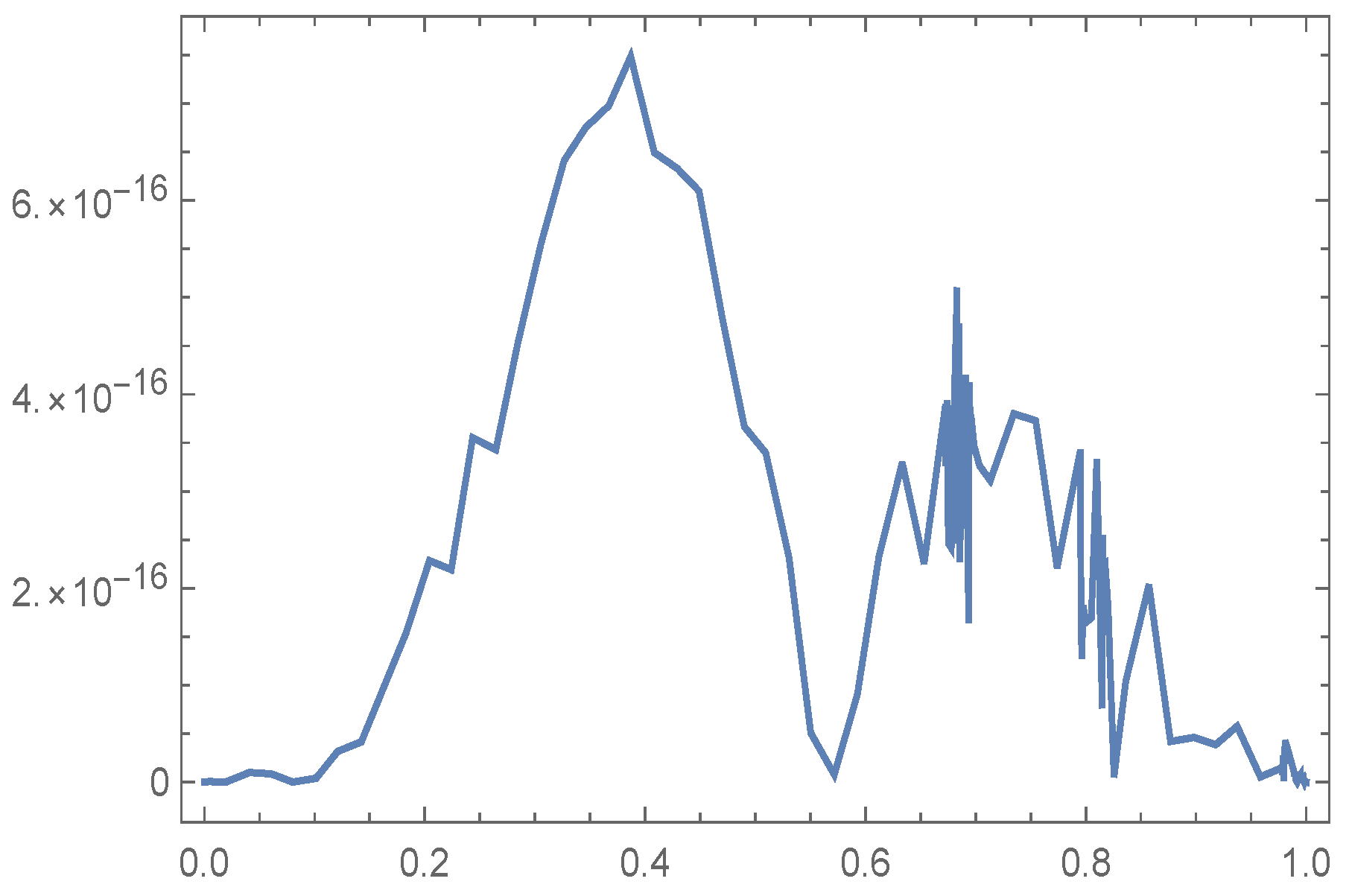
Example 1.

Consider the following eighth-order BVP [44,45,46,47]:

$$u^{\left(8\right)}\left(x\right)-u\left(x\right)=-8(2xcosx+7sinx),x\in [0,1],$$

(40)

$$\begin{array}{cc}\hfill & u\left(0\right)=0,u^{\prime }\left(0\right)=1,u^{″}\left(0\right)=0,u^{‴}\left(0\right)=-3,\hfill \\ \hfill & u\left(1\right)=0,u^{\prime }\left(1\right)=-e,u^{″}\left(1\right)=-4e,u^{‴}\left(1\right)=-9e,\hfill \end{array}$$

with the exact solution: $u\left(x\right)=x(1-x)e^x.$

We apply our algorithm—namely, SGJPGM—to solve problem (40).

Table 1. Comparison of $L^{\infty }$- and $L^2$-errors of our algorithm with distinct N for Example 1.

N	${\mathit{L}}^{\mathit{\infty }}$-Errors	${\mathit{L}}^2$-Errors
1	$4.48011·{10}^{-7}$	$2.44031·{10}^{-7}$
2	$4.30610·{10}^{-9}$	$2.13197·{10}^{-9}$
3	$1.65350·{10}^{-9}$	$8.88121·{10}^{-10}$
4	$1.02447·{10}^{-11}$	$5.64667·{10}^{-12}$
5	$1.35607·{10}^{-12}$	$7.03195·{10}^{-13}$
6	$7.02861·{10}^{-15}$	$3.89473·{10}^{-15}$
7	$8.40090·{10}^{-16}$	$3.46545·{10}^{-16}$

illustrates a comparison of $L^{\infty }$- and $L^2$-errors resulting from our algorithm with distinct N.

Table 2. Comparison of $L^{\infty }$-errors of our algorithm with those of methods in [44,45,46,47] for Example 1.

Error	SM in [44]	NPSM in [45]	RKM in [46]		LMM in [47]	SGJPGM
				$\mathit{N}=\mathbf{8}$	$\mathit{N}=\mathbf{10}$	$\mathit{N}=\mathbf{7}$
E	$1.20·{10}^{-5}$	$1.02·{10}^{-8}$	$4.90·{10}^{-9}$	$8.95·{10}^{-14}$	$2.85·{10}^{-16}$	$8.40·{10}^{-16}$

compares $L^{\infty }$-errors resulting from our algorithm with those resulting from the application of the following methods:

• The spline method (SM) in [44].
• The non-polynomial spline method (NPSM) in [45].
• The reproducing kernel method (RKM) in [46].
• The Legendre matrix method (LMM) in [47].

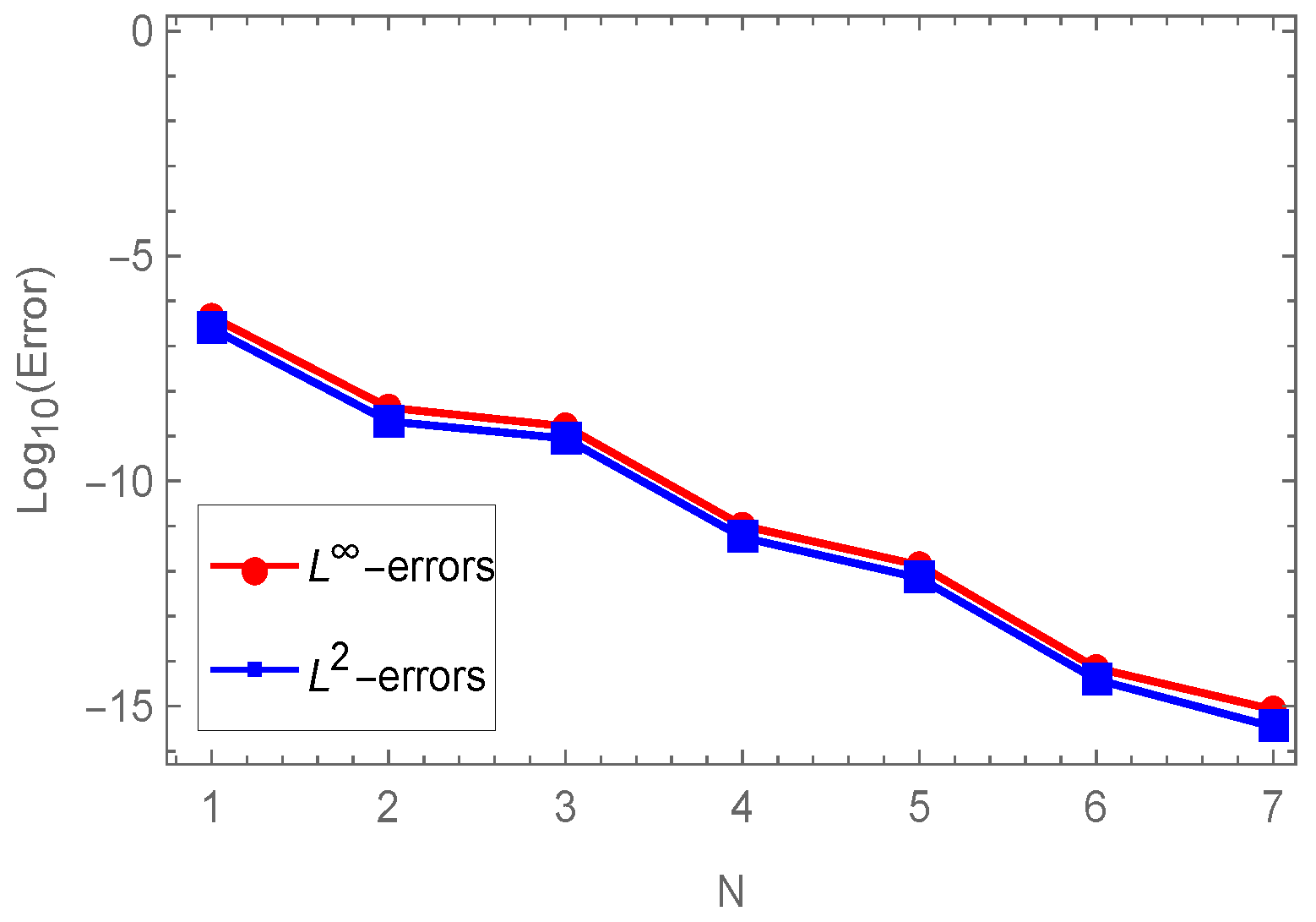
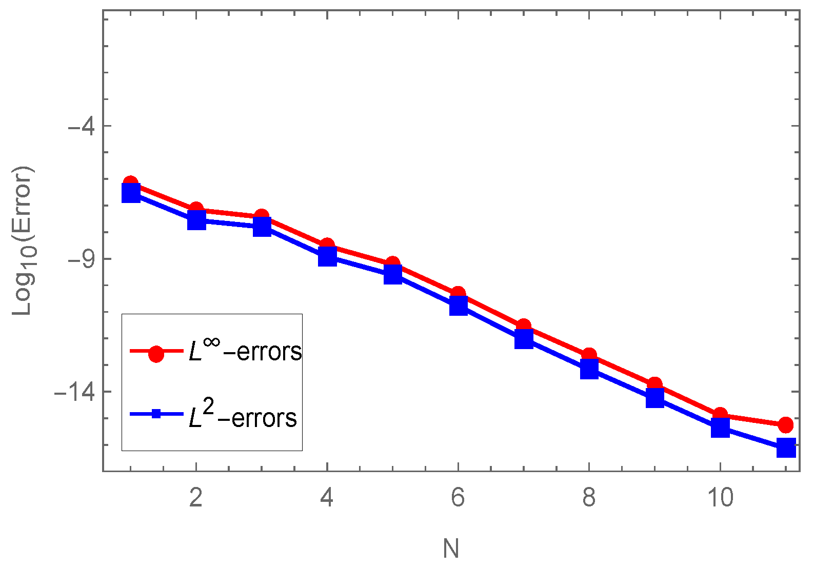
Furthermore, Figure 1 shows the MAEs of our algorithm at $N=7$, while Figure 2 shows the $Lo{g}_{10}(L^{\infty }$-errors) and $Lo{g}_{10}(L^2$-errors) of our algorithm with distinct N.

Example 2.

Consider the following BVP: [44,45,46]:

$$u^{\left(8\right)}\left(x\right)-u\left(x\right)=-8(2xcosx+7sinx),x\in [-1,1],$$

(41)

$$\begin{array}{cc}\hfill & u(-1)=0,u^{\prime }(-1)=2sin\left(1\right),u^{″}(-1)=-4cos\left(1\right)-2sin\left(1\right),u^{‴}(-1)=6cos\left(1\right)-6sin\left(1\right),\hfill \\ \hfill & u\left(1\right)=0,u^{\prime }\left(1\right)=2sin\left(1\right),u^{″}\left(1\right)=4cos\left(1\right)+2sin\left(1\right),u^{‴}\left(1\right)=6cos\left(1\right)-6sin\left(1\right),\hfill \end{array}$$

with the exact solution: $u\left(x\right)=(x^2-1)sinx.$

Our proposed method (SGJPGM) is applied to solve problem (41).

Table 3. Comparison of $L^{\infty }$ and $L^2$-errors of our algorithm with distinct N for Example 2.

N	${\mathit{L}}^{\mathit{\infty }}$-Errors	${\mathit{L}}^2$-Errors
1	$3.72783·{10}^{-6}$	$3.16549·{10}^{-6}$
3	$4.44508·{10}^{-8}$	$3.73237·{10}^{-8}$
5	$1.28602·{10}^{-10}$	$1.05002·{10}^{-10}$
7	$1.10634·{10}^{-13}$	$8.23261·{10}^{-14}$
9	$5.00745·{10}^{-14}$	$3.73238·{10}^{-14}$

illustrates a comparison of $L^{\infty }$- and $L^2$-errors of SGJPGM for various values of N.

Table 4. Comparison of $L^{\infty }$-errors of our algorithm with those of methods in [44,45,46] for Example 2.

Error	SM in [44]	NPSM in [45]	RKM in [46]	SGJPGM
	$\mathit{h}=\mathbf{1}/\mathbf{32}$	$\mathit{h}=\mathbf{1}/\mathbf{32}$	$\mathit{N}=\mathbf{10}$	$\mathit{N}=\mathbf{9}$
E	$1.20·{10}^{-5}$	$1.02·{10}^{-8}$	$4.90·{10}^{-9}$	$5.01·{10}^{-14}$

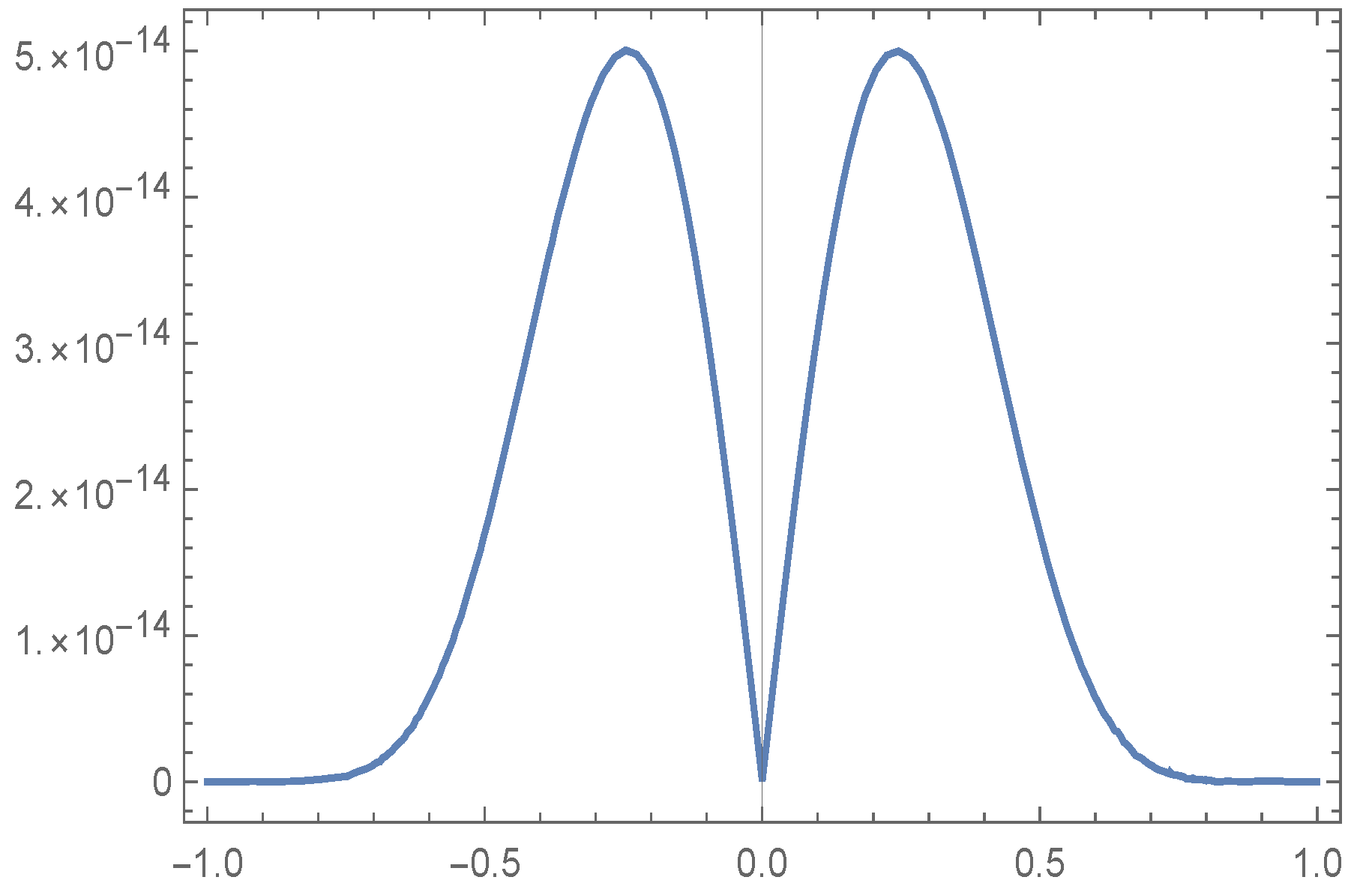
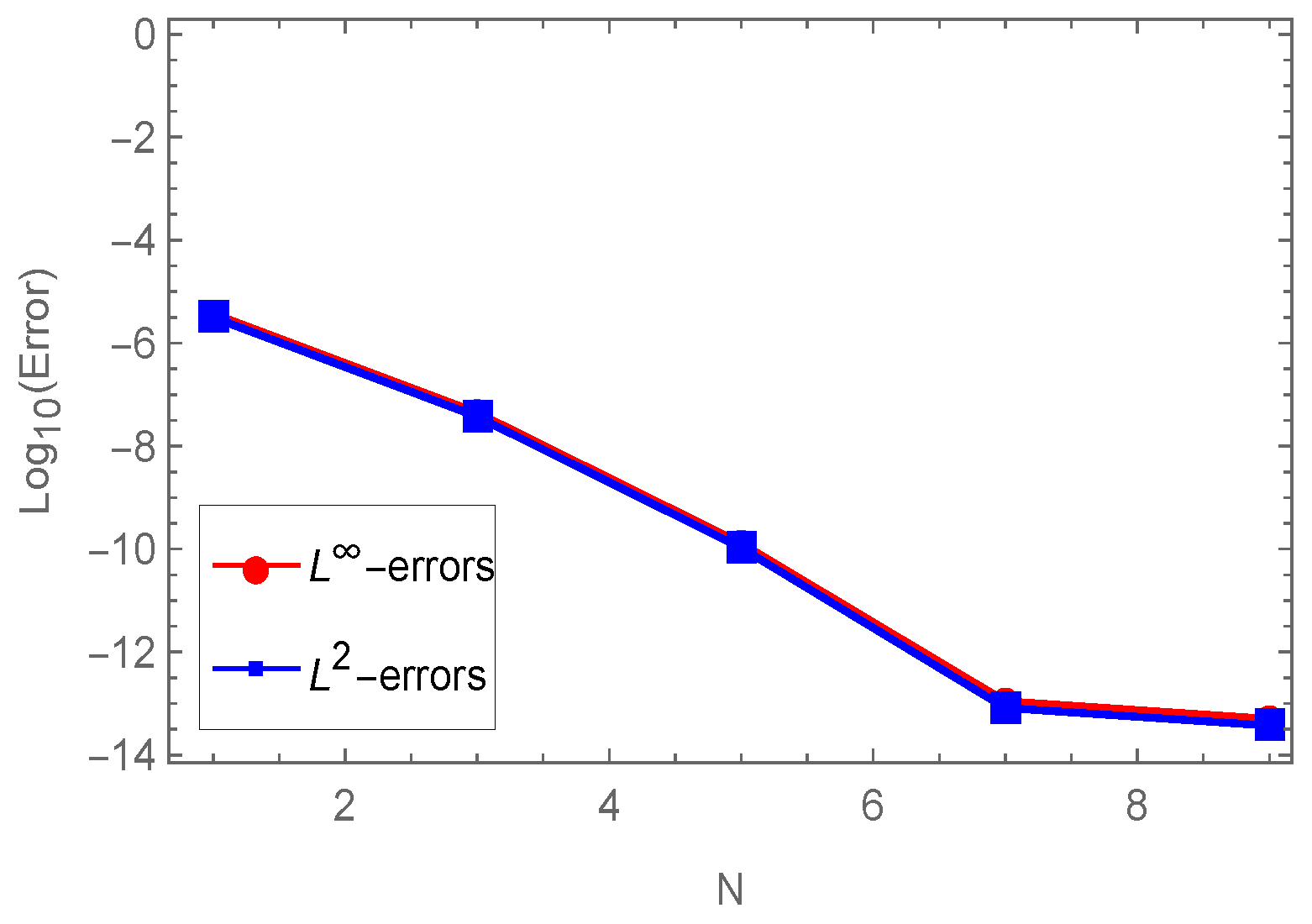
compares the $L^{\infty }$-errors resulting from our algorithm with those obtained if the methods in [44,45,46] are applied. In addition, Figure 3 displays the MAEs of our algorithm for $N=9$, while Figure 4 shows the $Lo{g}_{10}(L^{\infty }$-errors) and $Lo{g}_{10}(L^2$-errors) of our algorithm with distinct N.

Example 3.

Consider the BVP [48,49]:

$$Z^{\left(8\right)}\left(x\right)=7!\left(e^{-8Z\left(x\right)}-\frac{2}{{(x+1)}^8}\right),x\in [0,e^{1/2}-1],$$

(42)

subject to the BCs

$$\begin{array}{cc}\hfill & Z\left(0\right)=0,Z^{\prime }\left(0\right)=1,Z^{″}\left(0\right)=-1,Z^{‴}\left(0\right)=2,\hfill \\ \hfill & Z(e^{1/2}-1)=\frac{1}{2},Z^{\prime }(e^{1/2}-1)=e^{-1/2},Z^{″}(e^{1/2}-1)=-e^{-1},Z^{‴}(e^{1/2}-1)=2e^{-3/2},\hfill \end{array}$$

with the exact solution: $Z\left(x\right)=ln(x+1).$

Our proposed method—namely, SGJOMM—is applied to solve problem (42).

Table 5. Comparison of $L^{\infty }$- and $L^2$-errors of our algorithm with distinct N for Example 3.

N	${\mathit{L}}^{\mathit{\infty }}$-Errors	${\mathit{L}}^2$-Errors
1	$6.49854·{10}^{-7}$	$2.84248·{10}^{-7}$
2	$6.84114·{10}^{-8}$	$2.77812·{10}^{-8}$
3	$3.70217·{10}^{-8}$	$1.58289·{10}^{-8}$
4	$3.01981·{10}^{-9}$	$1.17252·{10}^{-9}$
5	$6.13366·{10}^{-10}$	$2.45326·{10}^{-10}$
6	$4.58591·{10}^{-11}$	$1.65191·{10}^{-11}$
7	$2.76063·{10}^{-12}$	$9.38161·{10}^{-13}$
8	$2.24598·{10}^{-13}$	$6.82216·{10}^{-14}$
9	$1.78746·{10}^{-14}$	$5.54010·{10}^{-15}$
10	$1.27676·{10}^{-15}$	$4.29149·{10}^{-16}$
11	$5.55112·{10}^{-16}$	$7.43891·{10}^{-17}$

illustrates a comparison of $L^{\infty }$- and $L^2$-errors of SGJOMM for various values of N.

Table 6. Comparison of $L^{\infty }$-errors of our algorithm with those of methods in [48,49] for Example 3.

Error	GSBSM in [48]	SGM in [49]	SGJOMM
			$\mathit{N}=\mathbf{11}$
E	$8.508563·{10}^{-5}$	$1.2303·{10}^{-11}$	$5.55112·{10}^{-16}$

compares the $L^{\infty }$-errors resulting from our algorithm with those obtained by the following two methods:

• The Galerkin septic B-splines method (GSBSM) in [48].
• The Sinc–Galerkin method (SGM) in [49].

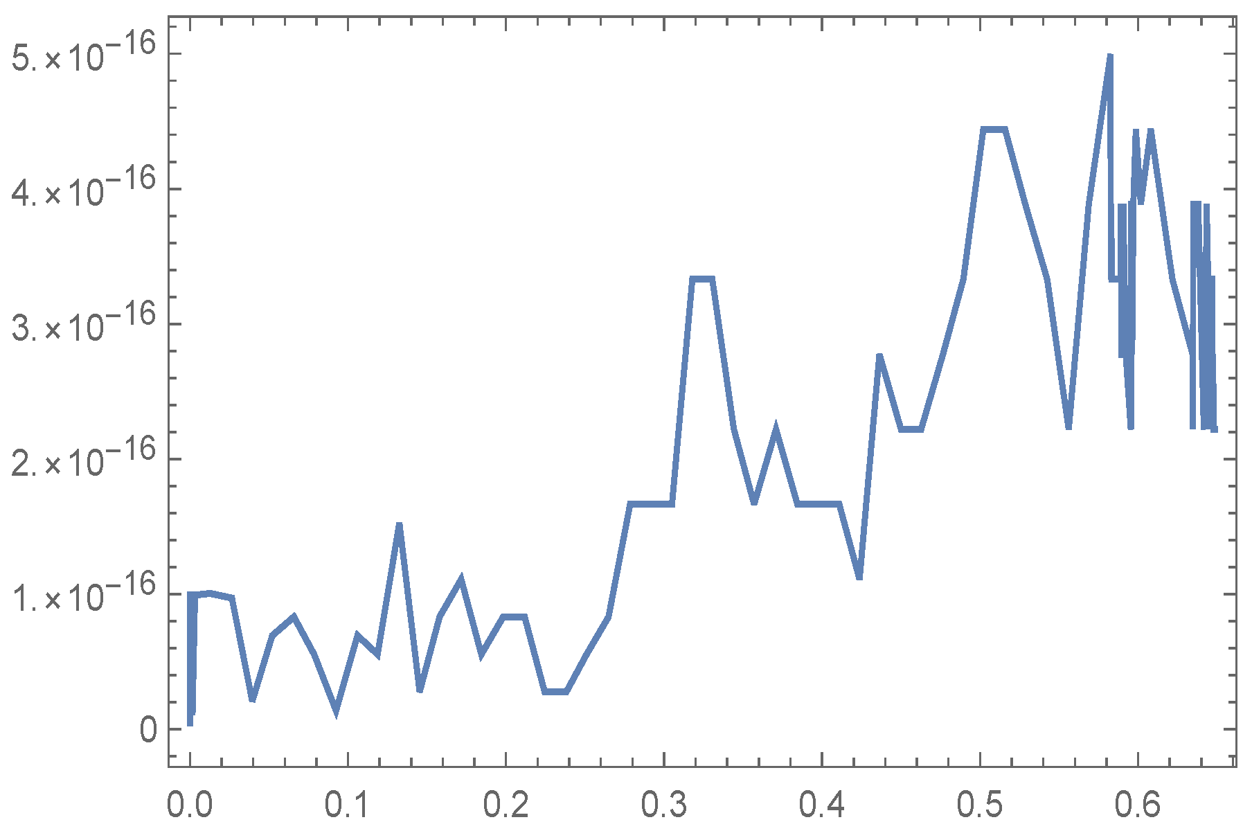
In addition, Figure 5 displays the MAEs of our algorithm at $N=11$, while Figure 6 shows the $Lo{g}_{10}(L^{\infty }$-errors) and $Lo{g}_{10}(L^2$-errors) of our algorithm with distinct N.

Example 4.

Consider the following non-linear two-point BVP [50,51]:

$$Z^{\left(4\right)}\left(x\right)+{\left(Z^{″}\left(x\right)\right)}^2=sinx+{sin}^{2}x,x\in [0,1],$$

(43)

subject to the BCs:

$$\begin{array}{cc}\hfill & Z\left(0\right)=0,Z^{\prime }\left(0\right)=1,\hfill \\ \hfill & Z\left(1\right)=sin\left(1\right),Z^{\prime }\left(1\right)=cos\left(1\right),\hfill \end{array}$$

with the following exact solution: $Z\left(x\right)=sinx.$

SGJOMM is applied to solve problem (43).

Table 7. Comparison of $L^{\infty }$- and $L^2$-errors of our algorithm by using Legendre, Chebyshev, and ${\tilde{R}}_j^{(2,2)}\left(x\right)$ with distinct N for Example 4.

	Legendre		Chebyshev		${\tilde{\mathit{R}}}_{\mathit{j}}^{(2,2)}\left(\mathit{x}\right)$
$\mathit{N}$	${\mathit{L}}^{\infty }$-Errors	${\mathit{L}}^{\mathbf{2}}$-Errors	${\mathit{L}}^{\infty }$-Errors	${\mathit{L}}^{\mathbf{2}}$-Errors	${\mathit{L}}^{\infty }$-Errors	${\mathit{L}}^{\mathbf{2}}$-Errors
1	$3.099·{10}^{-5}$	$1.917·{10}^{-5}$	$1.814·{10}^{-5}$	$1.099·{10}^{-5}$	$1.594·{10}^{-6}$	$8.994·{10}^{-7}$
2	$8.634·{10}^{-7}$	$5.173·{10}^{-7}$	$5.665·{10}^{-7}$	$3.354·{10}^{-7}$	$8.568·{10}^{-8}$	$4.853·{10}^{-8}$
3	$4.630·{10}^{-8}$	$2.536·{10}^{-8}$	$1.747·{10}^{-8}$	$8.598·{10}^{-9}$	$1.416·{10}^{-9}$	$7.770·{10}^{-10}$
4	$1.040·{10}^{-9}$	$5.920·{10}^{-10}$	$4.779·{10}^{-10}$	$2.553·{10}^{-10}$	$6.677·{10}^{-11}$	$3.720·{10}^{-11}$
5	$1.177·{10}^{-11}$	$5.603·{10}^{-12}$	$5.177·{10}^{-12}$	$2.726·{10}^{-12}$	$9.008·{10}^{-13}$	$4.917·{10}^{-13}$
6	$3.471·{10}^{-13}$	$1.820·{10}^{-13}$	$1.712·{10}^{-13}$	$9.264·{10}^{-14}$	$3.603·{10}^{-14}$	$1.983·{10}^{-14}$
7	$3.886·{10}^{-15}$	$1.757·{10}^{-15}$	$2.442·{10}^{-15}$	$9.810·{10}^{-16}$	$4.996·{10}^{-16}$	$2.212·{10}^{-16}$
8	$2.220·{10}^{-16}$	$5.449·{10}^{-17}$	$2.220·{10}^{-16}$	$3.080·{10}^{-17}$	$2.220·{10}^{-16}$	$7.638·{10}^{-18}$
9	$2.220·{10}^{-16}$	$4.844·{10}^{-19}$	$2.220·{10}^{-16}$	$3.224·{10}^{-19}$	$2.220·{10}^{-16}$	$8.795·{10}^{-20}$
10	$2.220·{10}^{-16}$	$3.847·{10}^{-20}$	$2.220·{10}^{-16}$	$3.685·{10}^{-20}$	$2.220·{10}^{-16}$	$4.775·{10}^{-20}$

illustrates a comparison of $L^{\infty }$- and $L^2$-errors of SGJOMM for various values of N using the following three types of collocation points:

• The zeros of the shifted Legendre polynomials.
• The zeros of the shifted Chebyshev polynomials of the first kind.
• The zeros of the shifted symmetric Jacobi polynomials ${\tilde{R}}_j^{(2,2)}\left(x\right)$.

Table 8. Comparison of $L^{\infty }$-errors of our algorithm by using Legendre, Chebyshev, and ${\tilde{R}}_j^{(2,2)}\left(x\right)$ at $N=7$ with those of methods in [50,51] for Example 4.

	VIM in [50]	DDM in [51]			Our Method
x			Legendre	Chebyshev	${\tilde{\mathit{R}}}_{\mathit{j}}^{(\mathbf{2},\mathbf{2})}\left(\mathit{x}\right)$
0.0	$9.5923·{10}^{-14}$	$1.6490·{10}^{-25}$	$0.0000·{10}^{-00}$	$0.0000·{10}^{-00}$	$0.0000·{10}^{-00}$
0.1	$7.7856·{10}^{-8}$	$1.2030·{10}^{-10}$	$6.1932·{10}^{-16}$	$3.2266·{10}^{-16}$	$1.7019·{10}^{-16}$
0.2	$2.7231·{10}^{-7}$	$4.0080·{10}^{-10}$	$5.2855·{10}^{-17}$	$6.7811·{10}^{-16}$	$2.5175·{10}^{-16}$
0.3	$5.2489·{10}^{-7}$	$7.3035·{10}^{-10}$	$2.6620·{10}^{-15}$	$1.1722·{10}^{-15}$	$2.0676·{10}^{-16}$
0.4	$7.7730·{10}^{-7}$	$1.0007·{10}^{-9}$	$3.8641·{10}^{-16}$	$2.2400·{10}^{-16}$	$1.8735·{10}^{-16}$
0.5	$9.7145·{10}^{-7}$	$1.1173·{10}^{-9}$	$3.7557·{10}^{-15}$	$2.3187·{10}^{-15}$	$4.1785·{10}^{-16}$
0.6	$1.0502·{10}^{-6}$	$1.0304·{10}^{-9}$	$2.0600·{10}^{-17}$	$2.7539·{10}^{-17}$	$2.4112·{10}^{-16}$
0.7	$9.6286·{10}^{-7}$	$7.6427·{10}^{-10}$	$2.8821·{10}^{-15}$	$1.1441·{10}^{-15}$	$8.8471·{10}^{-17}$
0.8	$6.8407·{10}^{-7}$	$4.1663·{10}^{-10}$	$1.9657·{10}^{-16}$	$9.5746·{10}^{-16}$	$3.7036·{10}^{-16}$
0.9	$2.7069·{10}^{-7}$	$1.2106·{10}^{-10}$	$6.6153·{10}^{-16}$	$2.7111·{10}^{-16}$	$3.0602·{10}^{-16}$
1.0	$1.5676·{10}^{-13}$	$1.4649·{10}^{-23}$	$0.0000·{10}^{-00}$	$0.0000·{10}^{-00}$	$0.0000·{10}^{-00}$

compares the $L^{\infty }$-errors resulting from our algorithm with those obtained by the following two methods:

• The variational iteration method (VIM) in [50].
• The double decomposition method (DDM) in [51].

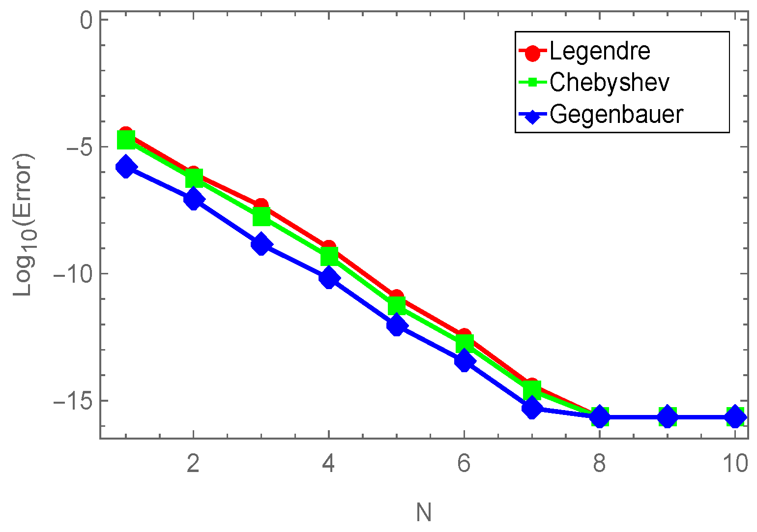
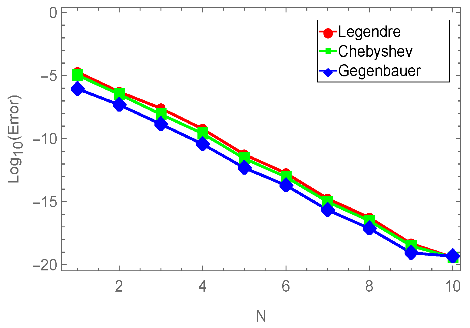
In addition, Figure 7 shows a comparison of $Lo{g}_{10}(L^{\infty }$-errors) of our algorithm by using Legendre, Chebyshev, and symmetric Jacobi polynomials with distinct N, while Figure 8 shows a comparison of $Lo{g}_{10}(L^2$-errors) of our algorithm by using (Legendre, Chebyshev, and symmetric Jacobi) with distinct N. using the same zeros.

8. Conclusions

A kind of orthogonal polynomial—namely, SGJPs—was utilized to treat both linear and non-linear BVPs. The linear ones were handled by applying the Petrov–Galerkin spectral method, while the non-linear ones were treated with the aid of the typical collocation method. To treat the linear BVPs, the expression for the derivatives of the SGJPs in terms of the shifted Legendre polynomials was established and utilized, while the algorithm designed for treating the non-linear BVPs was built on the utilization of the operational matrix of derivatives of the SGJPs. The two proposed numerical algorithms were tested via illustrative examples. These examples show the high performance and accuracy of the suggested algorithms. We also mention that the codes were written and debugged using Mathematica version 12 software using a PC machine, with Intel(R) Core(TM) i5-8500 CPU @ 3.00 GHz, 12.00 GB of RAM.