
Symmetries and Dynamics of Generalized Biquaternionic Julia Sets Defined by Various Polynomials


Department of Fundamentals of Machinery Design, Faculty of Mechanical Engineering, Silesian University of Technology, Konarskiego 18A, 44-100 Gliwice, Poland
Symmetry 2023, 15(1), 43; https://doi.org/10.3390/sym15010043
Submission received: 16 November 2022
/
Revised: 12 December 2022
/
Accepted: 21 December 2022
/
Published: 23 December 2022
(This article belongs to the Special Issue Topological Dynamical Systems)
Abstract
:Higher-dimensional hypercomplex fractal sets are getting more and more attention because of the discovery of more and more interesting properties and visual aesthetics. In this study, the attention was focused on generalized biquaternionic Julia sets and a generalization of classical Julia sets, defined by power and monic higher-order polynomials. Despite complex and quaternionic Julia sets, their biquaternionic analogues are still not well investigated. The performed morphological analysis of 3D projections of these sets allowed for definition of symmetries, limit shapes, and similarities with other fractal sets of this class. Visual observations were confirmed by stability analysis for initial cycles, which confirm similarities with the complex, bicomplex, and quaternionic Julia sets, as well as manifested differences between the considered formulations of representing polynomials.
1. Introduction
The studies of Mandelbrot in the 1970s on the iterative equation:
defined previously by Julia and Fatou in their investigation of complex dynamic systems, resulted in the discovery of one of the most geometrically complicated fractal sets, which is known nowadays as the Mandelbrot set, or simply M-set. By variation of , the M-set consists of an infinite number of Julia (usually marked as J sets) and Fatou sets, varied by their connectivity. These studies of Mandelbrot were summarized in his famous book [1]. More information on the Julia and Mandelbrot sets, including the most important theorems, can be also found in [2]. However, in addition to the classical complex iteration mapping given by (1), a generalization of (1) can be found in quaternions , the 4-dimensional hypercomplex algebra, i.e., in this case in (1) . This is owing to the cooperation of Mandelbrot with Norton, who defined the quaternionic Mandelbrot-Julia (M-J) sets in terms of quaternions [3,4]. In parallel, Holbrook [5] performed further investigations in terms of their symmetries and connectivity.
In the following decades, numerous generalizations of M-J sets in terms of hypercomplex number spaces were developed. They include the next logical step in the hypercomplex generalization of the M-J sets, that is, their generalization in terms of octonions (the 8-dimensional hypercomplex algebra), proposed by Griffin and Joshi [6] with further investigation of their properties [7,8], namely, the structural transitions characteristics for a large class of octonionic maps. Further generalizations of M-J sets were not possible, since the hypercomplex algebra of 16-dimensional sedenions , being the next generalization after octonions, does not meet any of fundamental properties necessary for addition and multiplication in an iteration process (see (1)), namely, sedenions are not commutative, associative, and alternative. The same is applicable to all subsequent generalizations. A detailed analysis of these properties can be found in [9].
Later, several other interesting generalizations were presented. In particular, Dixon et al. [10] investigated higher-dimensional generalizations of quadratic polynomial M-J sets defined in hypercomplex Clifford algebras. In this study, the authors demonstrated the fractal nature and symmetry properties of higher-dimensional hypercomplex M-J sets. Wang and Sun [11] proposed a generalization in terms of the power of the polynomial (1) in quaternions, namely:
In this study, the authors demonstrated the symmetry properties of quaternionic M-J sets, including those with negative power p and the stability analysis of these sets. In later studies, Wang’s team also investigated hypercomplex generalizations defined in terms of power p as in (2) [12], which was an extension of previous studies by Dixon et al. [10].
The new family of generalizations of M-J sets was established by Rochon and his team. Their studies focused on generalizations in terms of tensor product algebras: he introduced bicomplex ( or ) M-J sets in [13], later studied by Wang and Song [14] as well, and further generalizations up to multicomplex M-J sets [15,16,17]. This short overview shows that the hypercomplex generalizations of M-J sets are currently being intensively studied by numerous research teams.
Proceeding to the generalization of M-J sets in terms of tensor product algebras, it was found that there exist M-J sets defined in biquaternions . The first introduction of biquaternionic M-J sets was given by Gintz [18], where he described the fundamentals of algebra of biquaternions and showed several renderings of 3D projections of these fractal sets. Later, Bogush et al. [19] presented their studies on the symmetry of biquaternionic J sets. Studies by the first author on biquaternionic fractal sets were established in [20], where their graphical representation and preliminary analysis based on comparison with other complex and hypercomplex J sets were presented. Furthermore, a more detailed analysis of these fractal sets was performed and described in [9,21], where some unique properties for these sets were demonstrated.
This paper aimed to perform a systematic analysis of the symmetry properties of biquaternionic J sets of type (2) and their additional polynomial variation, as well as to investigate their stability to confirm the observations made during morphological analysis of these sets. Morphological analysis and evaluation of stability for biquaternionic J sets are presented for the first time, which is the main novelty of the study. Moreover, biquaternionic J sets of type (2) were also defined and investigated for the first time.
The rest of the paper is organized as follows. Section 2 consists of fundamental properties of biquaternions, as well as basic operations necessary for constructing biquaternionic J sets, which was also presented in this section. Further, in Section 3, the results of a morphological analysis are presented, including the appearing symmetries in both types of the investigated J sets. The results of stability analysis of initial cycles are presented and discussed in Section 4. The main conclusions are derived in Section 5.
2. Preliminaries
2.1. Biquaternions and Their Properties
The algebra of biquaternions, proposed by Hamilton in 1844 as one of the alternatives to quaternions [9], is a tensor product of the field of complex numbers and quaternions ; therefore, it is sometimes called a complexified quaternion. It is a 4-algebra, which is isomorphic to and some Clifford algebras [22,23]. In symbolic form, a biquaternion can be presented in a complexified form:
or extended alternative form
where and are imaginary units, i.e., , .
The fundamental operations on biquaternions, such as addition and multiplication, are the same as for quaternions, i.e., the algebra of biquaternions is alternative. This means that multiplication is performed according to special rules according to their non-commutativity. To simplify these fundamental operations, one can apply the idempotent representation of biquaternions proposed in [24]:
where , , , , which makes it possible to add and multiply biquaternions element-wise, so that two biquaternions and , can be added and multiplied as follows:
The full list of properties and basic operations on biquaternions can be found in [25].
2.2. Julia Sets within Biquaternions
2.2.1. Power Polynomials
The generalized J sets defined within biquaternions in the form
were defined and analyzed in one of the previous author’s publications [21]. Moreover, the condition of was discussed there. The main definitions and theorems for biquaternionic J sets are followed below for consistency.
Definition 1.
The generalized “filled” J set, obtained while iterating recursive Equation (8) is mapped into the biquaternionic vector space with a limited trajectory of c, and
Theorem 1.
[21].
Proof of Theorem 1.
Let . For the recursive equation defined by (8) and , according to Definition 1, has a bounded orbit . Additionally, when one obtains
where , and , thus
Considering that is bounded when , and are also bounded when . Then, , , and , and [21]. □
2.2.2. Monic Higher-Degree Polynomials
To investigate the homeomorphisms of M-J sets in a complex plane, Branner and Fagella [26] introduced the family of monic higher-degree polynomials in the following form:
This allowed us to analyze the connectedness and complex dynamics of limbs and external rays in M-J sets. Later, Zireh investigated the properties of a family of polynomials of type (12) defined in bicomplex numbers in terms of connectedness [27]. From the defined theorems and their proofs presented in [27], it can easily be seen that the same applies for (12) defined in biquaternions; therefore, these theorems are omitted in this paper.
The fundamentals on biquaternionic operations and definitions of J sets defined within power and monic higher-degree polynomials are used for their implementation for visualization and morphology analysis purposes, as well as for analysis of stability of these fractal sets presented in Section 3 and Section 4, respectively.
3. Symmetry of Biquaternionic Julia Sets
The first results on the construction of biquaternionic J sets in [18] were an inspiration for further investigation of these fractal sets, and their preliminary analysis was performed in [20,21], which focused on investigation of the symmetry of well-known analogues of J sets on a complex plane as well as the connectedness of these sets. In the following study, a systematic analysis in terms of symmetry of biquaternionic J sets of both types presented in Section 2.2 is presented.
For analysis of the symmetry of biquaternionic J sets, their 3D projections onto are used. Following the previous visualization techniques commonly used for the representation of 4D fractal sets, see, e.g., [11,13,14,20,21], where the 3D projection is obtained by setting in the quadruplet (3) to 0. As shown, for example, in [11], this procedure does not cause a loss of generality.
All 3D projections of the biquaternionic J sets presented in this paper were prepared in ChaosPro 4.0 freeware software. To implement addition and multiplication operations on biquaternions according to the rules presented in Section 2.1, which are necessary for the construction of biquaternionic J sets according to (8) and (12), a new library was prepared in the native programming language in ChaosPro, which is based on C/C++.
3.1. Symmetry of Biquaternionic Julia Sets Defined by Power Polynomials
As shown in [21], biquaternionic J sets do not resemble their quaternionic or bicomplex analogues in terms of symmetry. Wang and Sun in [11] demonstrated the rotational symmetry of quaternionic J sets, whereas Rochon showed the quadrilateral symmetry of bicomplex J sets, which was confirmed in [21]. The conjecture of uniqueness of biquaternionic J sets in terms of their symmetry made in [18] was confirmed in further studies presented in [21].
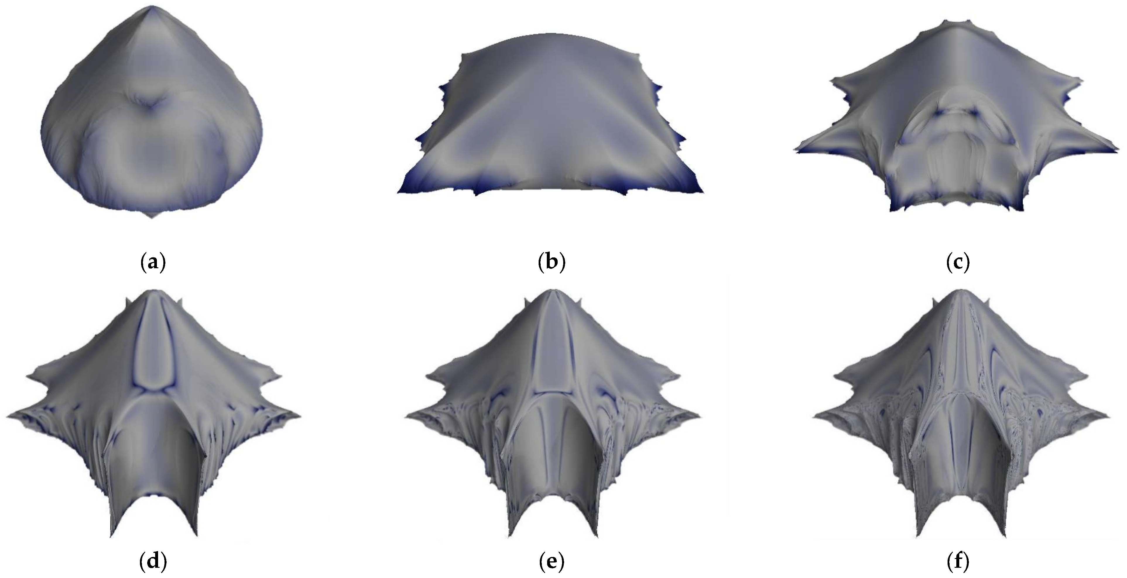
A simple way to show this uniqueness is to set in (8). The resulting recursion equation leads to the appearance of the analog of the so-called “unit disc” in the case of the -plane [4], i.e., . Previous studies on quaternionic and bicomplex J sets for such conditions [4,28,29] show that in the first case when one obtains a hypersphere (which was observed also in [11]), whereas in the second case, the resulting shape is a Steinmetz hypersolid. This can be generalized for their higher-dimensional analogues as well. To analyze the biquaternionic J sets for and increasing , their representative 3D projections are shown in Figure 1.
From the above projections, one can make the following observations on the properties of biquaternionic J sets.
Remark 1.
For J sets have nine planes of symmetry regardless of the value of .
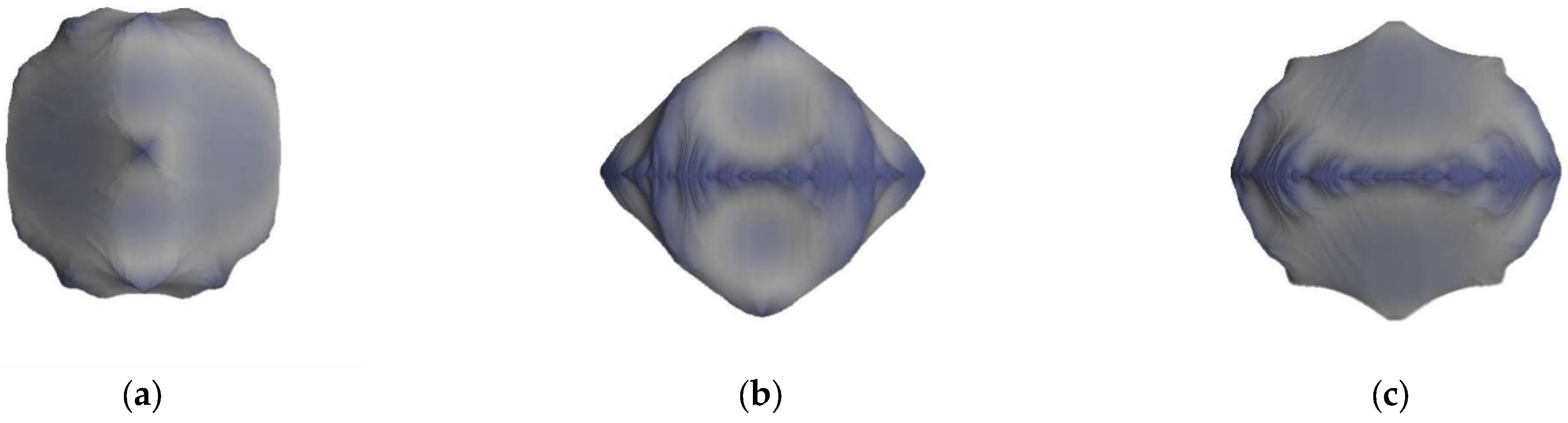
From the visualizations shown in Figure 1, the symmetry with respect to the plane in the coordinates defined as for a 3D projection ( is not taken into consideration) is well visible. To show the other symmetry planes, it is essential to visualize biquaternionic sets in other projections. Let us analyze the limit cases presented in Figure 1a,f. The orthogonal 3D projections are presented in Figure 2 and Figure 3, respectively, for and . Despite the increase in , the symmetry of biquaternionic J sets is preserved. One can observe that the symmetry of biquaternionic J sets is similar to that of bicomplex J sets (cf. the results presented in [29]).
Remark 2.
The shape of the biquaternionic J set tends to be a unique nontrivial set when .
As discussed earlier, for every M-J set of type (8) defined in a given number space tends to a set with a unique geometry characteristic for a given number space. Naturally, with an increase of , the value of has less influence and for it loses this influence completely. In the case of biquaternionic J sets, one can observe a unique shape of the J sets tend when , as seen in Figure 3. Because of the high value of one can consider this shape as very similar to the limit shape. The top 3D projection presented in Figure 3a depicts that this set contains characteristic horn-like structures, which are formed at the very beginning of the increase of (see Figure 1). Moreover, one can observe that the rotational symmetry in the plane is broken, i.e., the shape presented in Figure 3a is not the same if it is rotated by 90°. This is a direct consequence of the definition of these fractal sets in a hypercomplex number space composed from a tensor product of two dimensionally unequal algebras, .
Remark 3.
By reducing the number of non-zero elements in and , it is possible to obtain the analogues of the J sets defined in the -plane.
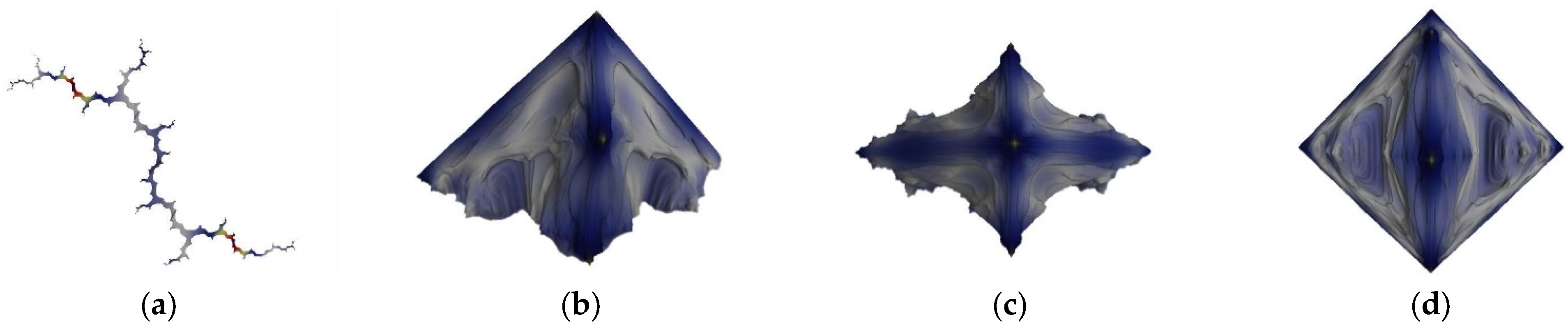
To visualize the relationship between biquaternionic and classical J sets defined in the -plane, it is essential to analyze sets with a specific geometry and values of , which demonstrate a similarity between the mentioned groups of fractal sets. The biquaternionic analogs of famous Dendrite and San Marco J sets are presented in Figure 4.
The Dendrite presented in Figure 4a shows a geometric structure characteristic for all types of number spaces used for construction of fractal sets (e.g., it looks like similar to J sets constructed in the -plane and -spaces as well as in the -space). The San Marco J set presented in Figure 4b–d in various projections reveals a much more complicated shape and it is difficult to observe its -plane analogue. The characteristic shape of the San Marco J set is quite visible in the top view (Figure 4c), which can be directly obtained by cutting its biquaternionic analogue in the plane. However, it is interesting to observe that in the plane (Figure 4d), this set has the form of a square. The lack of rotational symmetry typical for quaternionic or quadrilateral symmetry of bicomplex J sets as well as the above-discussed differences in various orthogonal projections is the result of a tensor product of dimensionally unequal algebras in the number space, where these sets were defined. However, the examples presented in Figure 4 proved that the biquaternionic J sets remain fractals.
3.2. Symmetry of Biquaternionic Julia Sets Defined by Monic Higher-Degree Polynomials
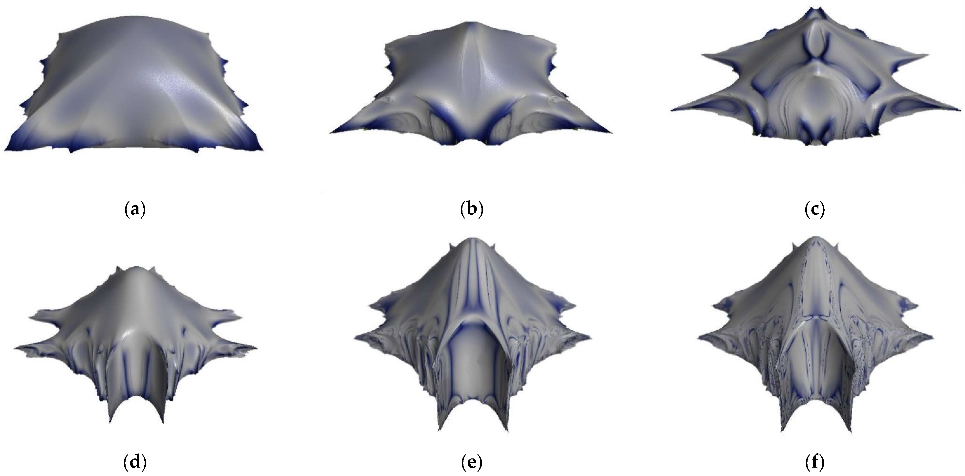
To investigate the homeomorphisms of J sets defined in biquaternions, the recurrence in Equation (12) is applied to generate visualizations with the same assumptions made in the preamble of Section 3 and Section 3.1. This allowed for observing the variability of the shapes of particular biquaternionic J sets defined by (12) with increasing as well as determining the limit shape when . The 3D projections of the J sets constructed using (12) for selected values of are presented in Figure 5.
From the above-presented visualizations, it can be observed that the resulting J sets for various values of reveal some differences, especially for low values of ; however, for higher values of , these differences become less and less recognizable. Finally, when , the resulting limit figure is the same as for the classical J set defined by (8), which is evident when substituting to to (8) and (12). Due to this, all symmetries characteristic for biquaternionic J sets defined by (8) are preserved.
Nevertheless, the dynamics of the biquaternionic J sets defined by (12) are completely different, which can be observed based on previously analyzed 3D projections of the analogues of Dendrite and San Marco fractals; see Figure 6. One can observe that the resulting shapes do not correspond to the biquaternionic J sets defined by (8), nor to their analogues defined in the -plane.
The J sets of both types, investigated from the point of view of their morphology and appearance symmetries, were further investigated in light of their stability, in particular, the determination of the boundaries of fixed points for variable , which is the subject of the next section.
4. Stability of Biquaternionic Julia Sets
In this section, the stability of generalized Julia sets defined in biquaternions is analyzed. The analysis was performed for both investigated recurrence Equations (8) and (12) for 1-, 2-, and 3-cycle stability and various values of , which made it possible to observe variation of stability for these sets when .
4.1. Stability of Biquaternionic Julia Sets Defined by Power Polynomials
4.1.1. 1-Cycle Stability
There are numerous similarities between biquaternions, quaternions, and bicomplex numbers; that is, all of these number spaces represent 4-dimenional hypercomplex numbers with numerous similar properties (see Section 2.1 for more details). Moreover, is isomorphic to [22]. Thus, the dynamics and stability of Julia sets defined as biquaternions are expected to reveal some similarities as in the case of their morphological analysis performed in Section 3.
Following [11,30], let us represent the n-th generation biquaternion in terms of Pauli matrices:
where is a set of 2 × 2 Pauli matrices:
completed by 2 × 2 invariant unit matrix
and , i.e., the biquaternion can be represented by its scalar and vector parts:
Note that for quaternions , i.e., the quaternion needs to be multiplied by and indices of need to be replaced (see, e.g., [25]), whereas for biquaternions, Pauli matrices (14) can be used directly without additional operations [31].
The recurrence relation for the biquaternionic quadratic map can be presented as:
where
Taking into account (13) and (16), we may write
The iterations of (17) considering (18) and (20) are represented by:
To determine fixed points and boundary regions for the biquaternionic quadratic map, it is necessary to determine the eigenvalues of the matrix with perturbed terms. Introducing the perturbation of , we have:
where is the so-called small perturbation parameter. This leads to:
which can be simplified to the following form:
where is the Landau symbol, which denotes truncation in terms of the order higher than the first one in solutions (27) and (28). Expanding in terms of the orthogonal triplet we have:
and omitting the Landau symbol in (27) and (28), we obtain:
From the matrix
we can determine considering (30) and (31):
which makes it possible to obtain the eigenvalues:
Considering that and noting that , the boundary region of the biquaternionic quadratic map is determined by
which leads to:
The boundary of the region of fixed points for the biquaternionic quadratic map is thus defined by:
In the same way, we can obtain solutions for higher-degree biquaternionic maps. Let us analyze the next cases discussed previously for and . The boundary region of fixed points for these cases are, respectively, as follows:
For detailed calculations for these cases, see Appendix A.
Taking into account (37) and (39)–(41), one can observe that these formulas lead to their general form proposed in [11] for quaternions:
Using (42), one can get the 1-cycle stability for the limit shape considered in the previous section. Substituting to (42), the direct result will have an indeterminate form; however, when representing it in terms of limits, we have
This confirms the convergence of the 1-cycle stability region of the generalized biquaternionic J set to the unit disc.
4.1.2. 2-Cycle Stability
The 2-cycle for the biquaternionic quadratic map is defined by the equation:
where is given by (18) and (19). Using the notation given by (13) and (16), the powers of can be given by (20) and the following expression:
The iterations of (45) considering (18), (20) and (46) are represented by:
From matrix (32) we can determine :
and the corresponding eigenvalues:
Taking the module of (54), we have:
which leads to the determination of the boundary of the region of fixed points for the 2-cycle using (37) and (38).
In a similar way, we can determine the boundary regions of fixed points for the 2-cycle for and , where:
The presentation of the detailed calculations was omitted in this paper because of its severe extension.
From the obtained values, one can derive the general formula for for the 2-cycle:
Assuming in (58), one leads to the conclusion that the 2-cycle stability region of the generalized biquaternionic J set also leads to the unit disc.
4.1.3. 3-Cycle Stability
Starting again from the biquaternionic quadratic map, the 3-cycle analogue is defined by the equation:
where is given by (18) and (19). Using the notation given by (13) and (16), the powers of can be given by (20), (46), and the following expressions:
Introducing perturbation of and simplifications, which were omitted here due to complex notation, one obtains the matrix from which the eigenvalues are calculated. Taking the module of the obtained eigenvalues, we have:
Using a similar procedure, the value of was calculated for :
Calculations for the higher values of were not possible because of the hardware limitations. Because of this, the determination of the general formulas for the 3-cycle and higher cycles is not possible through the computational way. Nevertheless, it is expected that the dynamics are different for higher cycles, which finally leads to the limit shape observed in Section 3.1.
4.2. Stability of Biquaternionic Julia Sets Defined by Monic Higher-Degree Polynomials
4.2.1. 1-Cycle Stability
The recurrence relation for the biquaternionic quadratic map defined in terms of monic higher-degree polynomials (12) can be presented as:
Using the notation given by (13) and (16), the powers of can be given by (20) and (A1). Applying the same procedure as in Section 4.1.1, one can calculate the iterations of (64) considering (18), (20) and (46), which can be represented by:
Introducing the perturbation of and simplifications, we can obtain the eigenvalues in the following form:
Taking the module of (67), we have:
which leads to the determination of the boundary of the region of fixed points for a 1-cycle using (36) and (37).
Similarly, we can determine the boundary regions of fixed points for a 1-cycle for and , where:
4.2.2. 2-Cycle Stability
The 2-cycle for the biquaternionic quadratic map defined in terms of monic higher-degree polynomials (12) is given by equation:
The powers of are given by (20), (46), (60), (61), (A1), (A3), and the following expression:
Omitting the steps presented above, one leads to the determination of modules of eigenvalues for 2-cycle stability, which in this case have the following values for the considered :
4.2.3. 3-Cycle Stability
Finally, the 3-cycle for the biquaternionic quadratic map defined in terms of monic higher-degree polynomials (12) is given by the equation:
In this case, the powers of are given by all expressions mentioned in Section 4.2.2 and the following ones:
Using the same computational procedure as previously, the modulus of the eigenvalue for 3-cycle stability was determined for :
Because of the increasing computational complexity (for the maximal power within the polynomial is 48, while for this value equals 180), the determination of modules of eigenvalues for higher values of were not possible because of hardware limitations.
5. Conclusions
This paper discusses the generalized biquaternionic Julia sets defined by power and monic higher-degree polynomials in terms of their symmetry and stability. The 3D projections of both types of fractal sets were constructed and discussed. The symmetry planes for these fractal sets were defined together with the definition and analysis of the limit shapes (when ). The similarities between fractal sets were constructed based on power polynomials and its analogues in other hypercomplex number spaces with the same dimension, such as fractal sets defined in quaternions and bicomplex numbers. Moreover, it was shown that all of the mentioned fractal sets have the same origin as complex Julia sets. The biquaternionic Julia sets constructed based on monic higher-degree polynomials were presented for the first time, and the morphological analysis of these sets shows that their shapes and dynamics are completely different with respect to the above-discussed fractal sets defined in power polynomials, again underlining the multimodality and increasing complexity of Julia sets defined in hypercomplex number spaces.
To support the observations made during the morphological analysis, stability calculations were performed for both investigated types of fractal sets. It was shown that the dynamics of biquaternionic Julia sets defined by power polynomials reveal similarities to the dynamics of fractal sets defined in quaternions, at least in the initial cycles of stability. The severe differences between these two types of fractal sets are expected to appear at high cycles of stability; however, because of hardware limitations, these differences have not been identified yet. In contrast, the biquaternionic fractal sets defined by monic high-order polynomials reveal some similarities but different and more complex behavior, which confirms the observations made for the morphology of these sets.
Funding
This research received no external funding.
Data Availability Statement
Not applicable.
Conflicts of Interest
The author declares no conflict of interest.
List of Symbols
| complex elements of a biquaternion | |
| complex elements of a biquaternion | |
| constant value of the Julia/Mandelbrot set | |
| complex number space | |
| bicomplex number space | |
| multicomplex number space | |
| bicomplex number space | |
| biquaternion number space | |
| complex elements of the constant value of the biquaternionic Julia set | |
| vector part of constant value of the biquaternionic Julia set | |
| real elements of the extended representation of a biquaternion | |
| real elements of the extended representation of a biquaternion | |
| quaternion number space | |
| imaginary units | |
| invariant unit matrix | |
| imaginary unit | |
| generalized biquaternionic Julia set | |
| natural number space | |
| Landau symbol | |
| octonion number space | |
| power of the iterated variable of the Julia/Mandelbrot set | |
| biquaternion | |
| real number space | |
| scalar parts of the iterated variable of the biquaternionic Julia set | |
| sedenion number space | |
| complex elements of vector parts of biquaternions | |
| vector parts of the iterated variable of the biquaternionic Julia set | |
| complex elements of vector parts of the iterated variable of the biquaternionic Julia set | |
| complex elements of scalar parts of the iterated variable of the biquaternionic Julia set | |
| complex elements of vector parts of the iterated variable of the biquaternionic Julia set | |
| iterated variable of the Julia/Mandelbrot set | |
| small perturbation parameter | |
| eigenvalues | |
| biquaternionic root of −1 | |
| Pauli matrices | |
| arbitrary complex numbers | |
| symmetry plane along the axes of imaginary values and | |
| symmetry plane along the axes of reals and imaginary values | |
| symmetry plane along the axes of reals and imaginary values |
Appendix A
Considering the preliminaries given by (13)–(16), (18) and (19), one can calculate 1-cycle stability of the biquaternionic map for and . According to this, we obtain
Representing (A1) and (A2) as two parts, for , we have
and for
Introducing perturbation in the same way as in (23) and (24) and introducing the Landau symbol in the obtained solutions to truncate higher-order terms, for , we have
and for
Using (29) and omitting the Landau symbol, for , we obtain
and for
which leads to construction of matrix of the form (32) and determination of eigenvalues for
and for
Taking the module of (A15) and (A16) and noting that , for , we have
and for .
References
- Mandelbrot, B.B. The Fractal Geometry of Nature; Freeman and Company: New York, NY, USA, 1983. [Google Scholar]
- Falconer, K. Fractal Geometry: Mathematical Foundations and Applications, 3rd ed.; John Wiley and Sons: Chichester, UK, 2014. [Google Scholar]
- Norton, A.V. Generation and display of geometric fractals in 3-D. Comput. Graph. 1982, 16, 61–67. [Google Scholar] [CrossRef]
- Norton, A.V. Julia sets in the quaternions. Comput. Graph. 1989, 13, 267–278. [Google Scholar] [CrossRef]
- Holbrook, J.A.R. Quaternionic Fatou-Julia sets. Ann. Sci. Math. Que. 1987, 11, 79–94. [Google Scholar]
- Griffin, C.J.; Joshi, G.C. Octonionic Julia sets. Chaos Solitons Fract. 1992, 2, 11–24. [Google Scholar] [CrossRef]
- Griffin, C.J.; Joshi, G.C. Transition points in octonionic Julia sets. Chaos Solitons Fract. 1993, 3, 67–88. [Google Scholar] [CrossRef]
- Griffin, C.J.; Joshi, G.C. Associators in generalized octonionic maps. Chaos Solitons Fract. 1993, 3, 307–319. [Google Scholar] [CrossRef]
- Katunin, A. A Concise Introduction to Hypercomplex Fractals; CRC Press: Boca Raton, FL, USA, 2017. [Google Scholar]
- Dixon, S.L.; Steele, K.L.; Burton, R.P. Generation and graphical analysis of Mandelbrot and Julia sets in more than four dimensions. Comput. Graph. 1996, 20, 451–456. [Google Scholar] [CrossRef]
- Wang, X.Y.; Sun, Y.Y. The general quaternionic M-J sets on the mapping z ← zα + c (α ∈ N). Comput. Math. Appl. 2007, 53, 1718–1732. [Google Scholar] [CrossRef] [Green Version]
- Wang, X.Y.; Jin, T. Hyperdimensional generalized M–J sets in hypercomplex number space. Nonlinear Dyn. 2013, 73, 843–852. [Google Scholar] [CrossRef]
- Rochon, D. A generalized Mandelbrot set for bicomplex numbers. Fractals 2000, 8, 355–368. [Google Scholar] [CrossRef]
- Wang, X.Y.; Song, W.J. The generalized M–J sets for bicomplex numbers. Nonlinear Dyn. 2013, 72, 17–26. [Google Scholar] [CrossRef]
- Garant-Pelletier, V.; Rochon, D. On a generalized Fatou-Julia theorem in multicomplex spaces. Fractals 2009, 17, 241–255. [Google Scholar] [CrossRef]
- Parisé, P.O.; Rochon, D. A study of dynamics of the tricomplex polynomial ηp + c. Nonlinear Dyn. 2015, 82, 157–171. [Google Scholar] [CrossRef]
- Brouillette, G.; Rochon, D. Characterization of the principal 3D slices related to the multicomplex Mandelbrot set. Adv. Appl. Clifford Algebr. 2019, 29, 39. [Google Scholar] [CrossRef] [Green Version]
- Gintz, T.W. Artist’s statement CQUATS—A non-distributive quad algebra for 3D renderings of Mandelbrot and Julia sets. Comput. Graph. 2002, 26, 367–370. [Google Scholar] [CrossRef]
- Bogush, A.A.; Gazizov, A.Z.; Kurochkin, Y.A.; Stosui, V.T. Symmetry properties of quaternionic and biquaternionic analogs of Julia sets. Ukr. J. Phys. 2003, 48, 295–299. [Google Scholar]
- Katunin, A. Analysis of 4D hypercomplex generalizations of Julia sets. In Proceedings of the Computer Vision and Graphics, Warsaw, Poland, 19–21 September 2016; Chmielewski, L.J., Datta, A., Kozera, R., Wojciechowski, K., Eds.; Lecture Notes in Computer Science. Springer: Cham, Switzerland, 2016; Volume 9972, pp. 627–635. [Google Scholar]
- Katunin, A. The generalized biquaternionic M-J sets. J. Geom. Graph. 2018, 22, 49–58. [Google Scholar]
- Rosenfeld, B. Geometry of Lie Groups; Springer: Dordrecht, The Netherlands, 1997. [Google Scholar]
- Francis, M.R.; Kosowsky, A. The construction of spinors in geometric algebra. Ann. Phys. 2005, 317, 383–409. [Google Scholar] [CrossRef] [Green Version]
- Sangwine, S.J.; Alfsmann, D. Determination of the biquaternion divisors of zero, including the idempotents and nilpotents. Adv. Appl. Clifford Algebr. 2010, 20, 401–410. [Google Scholar] [CrossRef] [Green Version]
- Sangwine, S.J.; Ell, T.A.; Le Bihan, N. Fundamental representations and algebraic properties of biquaternions or complexified quaternions. Adv. Appl. Clifford Algebras 2011, 21, 607–636. [Google Scholar] [CrossRef] [Green Version]
- Branner, B.; Fagella, N. Homeomorphisms between limbs of the Mandelbrot set. J. Geom. Anal. 1999, 9, 327–390. [Google Scholar] [CrossRef] [Green Version]
- Zireh, A. A generalized Mandelbrot set of polynomials of type Ed for bicomplex numbers. Georgian Math. J. 2008, 15, 189–194. [Google Scholar] [CrossRef]
- Katunin, A.; Fedio, K. On a visualization of the convergence of the boundary of generalized Mandelbrot set to (n − 1)-sphere. J. Appl. Math. Comput. Mech. 2015, 14, 63–69. [Google Scholar] [CrossRef]
- Katunin, A. On the convergence of multicomplex M-J sets to the Steinmetz hypersolids. J. Appl. Math. Comput. Mech. 2016, 15, 67–74. [Google Scholar] [CrossRef] [Green Version]
- Gomatam, J.; Doyle, J.; Steves, B.; McFarlane, I. Generalization of the Mandelbrot set: Quaternionic quadratic maps. Chaos Solitons Fract. 1995, 5, 971–986. [Google Scholar] [CrossRef]
- Berezin, A.V.; Kurochkin, U.A.; Tolkachov, E.A. Quaternions in Relativistic Physics, 2nd ed.; Editorial URSS: Moscow, Russia, 2003. [Google Scholar]
Figure 1.
Three-dimensional projections of biquaternionic J sets obtained from (8) for and various values of , a perspective view. (a) , (b) , (c) , (d) , (e) , (f) .
Figure 1.
Three-dimensional projections of biquaternionic J sets obtained from (8) for and various values of , a perspective view. (a) , (b) , (c) , (d) , (e) , (f) .

Figure 2.
Three-dimensional projections of various of biquaternionic J sets obtained from (8) for and : (a) plane, (b) plane, (c) plane.
Figure 2.
Three-dimensional projections of various of biquaternionic J sets obtained from (8) for and : (a) plane, (b) plane, (c) plane.

Figure 3.
Three-dimensional projections of various biquaternionic J sets obtained from (8) for and : (a) plane, (b) plane, (c) plane.
Figure 3.
Three-dimensional projections of various biquaternionic J sets obtained from (8) for and : (a) plane, (b) plane, (c) plane.

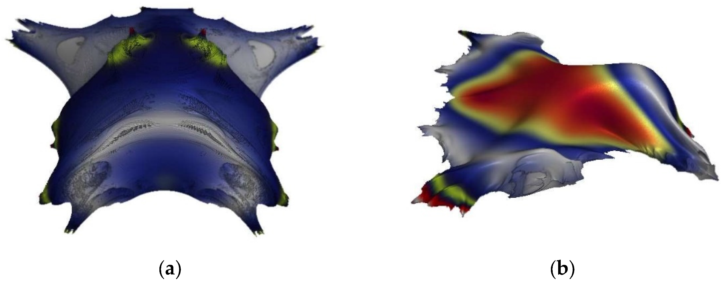
Figure 4.
Three-dimensional projections of characteristic biquaternionic J sets obtained from (8) for Dendrite , (a), San Marco , in isometric (b), top (c), and side (d) views, respectively.
Figure 4.
Three-dimensional projections of characteristic biquaternionic J sets obtained from (8) for Dendrite , (a), San Marco , in isometric (b), top (c), and side (d) views, respectively.

Figure 5.
Three-dimensional projections of biquaternionic J sets generated with monic higher-degree polynomials (12) for and various values of , a perspective view. (a) , (b) , (c) , (d) , (e) , (f) .
Figure 5.
Three-dimensional projections of biquaternionic J sets generated with monic higher-degree polynomials (12) for and various values of , a perspective view. (a) , (b) , (c) , (d) , (e) , (f) .

Figure 6.
Three-dimensioanl projections of biquaternionic J sets generated with monic higher-degree polynomials (12) for Dendrite , (a), and San Marco , (b), in isometric views.
Figure 6.
Three-dimensioanl projections of biquaternionic J sets generated with monic higher-degree polynomials (12) for Dendrite , (a), and San Marco , (b), in isometric views.

Disclaimer/Publisher’s Note: The statements, opinions and data contained in all publications are solely those of the individual author(s) and contributor(s) and not of MDPI and/or the editor(s). MDPI and/or the editor(s) disclaim responsibility for any injury to people or property resulting from any ideas, methods, instructions or products referred to in the content. |
© 2022 by the author. Licensee MDPI, Basel, Switzerland. This article is an open access article distributed under the terms and conditions of the Creative Commons Attribution (CC BY) license (https://creativecommons.org/licenses/by/4.0/).
Share and Cite
MDPI and ACS Style
Katunin, A. Symmetries and Dynamics of Generalized Biquaternionic Julia Sets Defined by Various Polynomials. Symmetry 2023, 15, 43. https://doi.org/10.3390/sym15010043
AMA Style
Katunin A. Symmetries and Dynamics of Generalized Biquaternionic Julia Sets Defined by Various Polynomials. Symmetry. 2023; 15(1):43. https://doi.org/10.3390/sym15010043
Chicago/Turabian StyleKatunin, Andrzej. 2023. "Symmetries and Dynamics of Generalized Biquaternionic Julia Sets Defined by Various Polynomials" Symmetry 15, no. 1: 43. https://doi.org/10.3390/sym15010043
Note that from the first issue of 2016, this journal uses article numbers instead of page numbers. See further details here.