Nonlinear Adaptive Fuzzy Control Design for Wheeled Mobile Robots with Using the Skew Symmetrical Property

Abstract

This research presents a nonlinear adaptive fuzzy control method as an analytical design and a simple control structure for the trajectory tracking problem in wheeled mobile robots with skew symmetrical property. For this trajectory tracking problem in wheeled mobile robots, it is not easy to find an analytical adaptive fuzzy control solution due to the complicated error dynamics between the controlled wheeled mobile robots and desired trajectories. For deriving the analytical adaptive fuzzy control law of this trajectory tracking problem, a filter link is firstly adopted to find the solvable error dynamics, then the research is based on the skew symmetrical property of the transformed error dynamics. This proposed nonlinear adaptive fuzzy control solution has the advantages of low computational resource consumption and elimination of modeling uncertainties. From the results for tracking two simulation scenarios (an S type trajectory and a square trajectory), the proposed nonlinear adaptive fuzzy control method demonstrates a satisfactory trajectory tracking performance for the trajectory tracking problem in wheeled mobile robots with huge modeling uncertainties and outperforms the existing H₂ control method.

1. Introduction

The broad applications of wheeled mobile robots (WMRs) with a skew symmetrical property have been attracting much attention because WMRs have been becoming more and more important for assisting daily human life and industry operations in recent years. These WMRs need to have a precise motion ability and effective control methods to achieve assigned missions [1,2,3,4,5]. Much of the literature on WMRs for trajectory tracking control have been focused on fuzzy control [6,7,8,9], neural networks control [10,11,12], sliding mode control [13,14,15,16], backstepping control [17,18,19], and feedback linearization control [20,21,22]. However, in real applications, successfully implementing the above proposed control methods requires huge design efforts due to controller complexities. Thus, an effective optimal control with a simple and easy-to-implement control structure is important for controlled WMR, and there are several related research works on this [23,24,25,26]. For the above issue, a simple optimal control structure should be developed, and this issue can be fixed with a closed-form solution or analytical solution for this optimal trajectory tracking problem. However, it is a difficult task for the trajectory tracking problem of the WMR to obtain a closed-form solution or analytical solution due to complex error dynamics. Fortunately, using a suitable mathematical arrangement, the closed-form solution or an analytical solution can be derived. In practice, the WMR must work under modelling uncertainties due to variations of payload and energy loss. Therefore, an innovative nonlinear adaptive fuzzy optimal control method that is a closed-form design will compensate for the issue of system parameter variations for the optimal trajectory tracking problem of the WMR in this investigation. Adaptive fuzzy control designs with parameters of on-line learning ability have been widely used in many applications. For example, a neural network based adaptive control design was proposed for dealing with nonlinear nonaffine systems with modeling uncertainties [27]; a trajectory-tracking and path-following design was developed for underactuated autonomous vehicles with parametric modeling uncertainty [28]; an iterative learning control (ILC) of constrained multi-input multi-output (MINO) nonlinear systems under the state alignment condition with varying trail lengths was developed to meet the alignment condition by adjusting the reference trajectory [29]; and a data-driven control of networked nonlinear systems with event-triggered output was proposed by integrating the estimated disturbances, the true and the estimated tracking error and the resultant tracking error systems, which were uniformly ultimately bounded [30]. These published results indicate the powerful modeling elimination capability of adaptive control laws with on-line parameter learning ability. For these reasons, for tackling varying system parameters of the WMR, a parameterized formulation is used on-line to precisely estimate time-varying system parameters, including mass, inertia, etc., in this investigation. This proposed adaptive fuzzy control law facilities engineers and researchers to realize control design of the WMR practically, because it is a closed-form solution and has the simplest control structure. Due to these promising characteristics, this centralized control law will possess a low calculation consumption and thus save energy. Furthermore, this proposed method can mitigate the effect of varying modelling uncertainties based on the on-learning ability of the derived adaptive fuzzy control law for system parameters. This research is arranged as follows. Section 1 presents the introduction and literature review. In Section 2, the wheeled mobile robot dynamics are described. Section 3 presents the adaptive fuzzy with H₂ control design. Section 4 illustrates the simulation results obtained for tracking the S type and square trajectory by adopting the proposed adaptive fuzzy control method and the H₂ control method. Finally, the conclusions are given in Section 5.

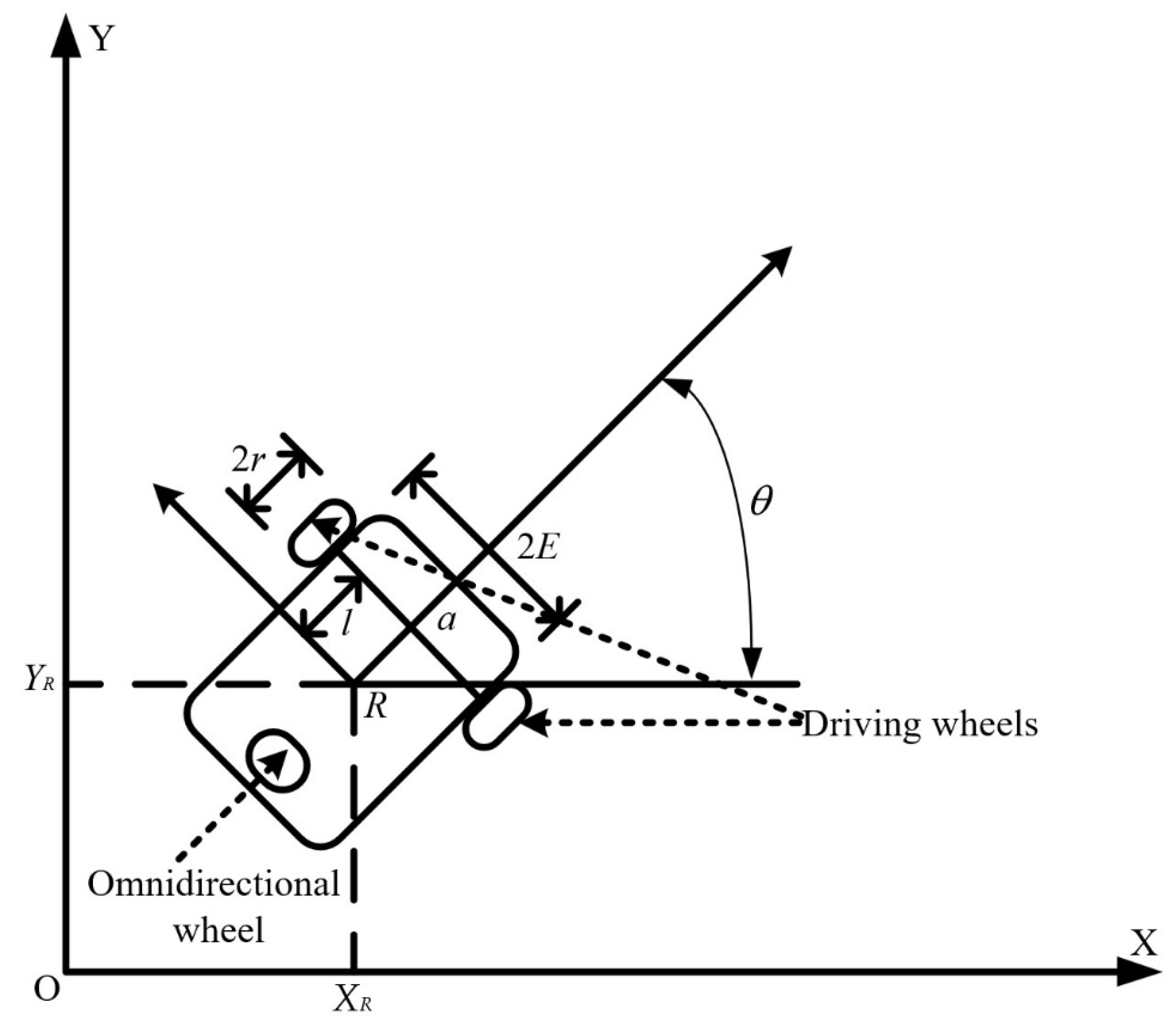
2. Wheeled Mobile Robot Dynamics

In this section, the WMR dynamics are described and the error dynamics of trajectory tracking with the desired trajectory are also formulated.

2.1. Wheeled Mobile Robot Dynamics

A wheeled mobile robot which consists of two driving wheels and one omnidirectional wheel is shown in Figure 1. Two driving wheels of the WMR are separated by 2E and both two driving wheels have the same radius of r. The instantaneous position of this controllable WMR in the global coordinate frame {O, X, Y} is denoted as $a$. R = ($x_R$,$y_R$) presents the position of the controllable WMR in the global coordinate frame, and the angle θ denotes the direction of the local frame {R, X_R, Y_R}. Based on the above descriptions, the global coordinate frame of the WMR will be expressed by Equation (1).

$$a={[\begin{array}{ccc}{x}_R& y_R& \theta \end{array}]}^T$$

(1)

The dynamic system of the WMR is illustrated in Figure 1 and this WMR usually moves heading toward the direction of the axis of the driving wheels. Then, the kinematics of the WMR with constraints can be presented as Equation (2).

$$\dot{a}=\left[\begin{array}{c}{\dot{x}}_R\\ {\dot{y}}_R\\ \dot{\theta }\end{array}\right]=\left[\begin{array}{cc}\cos \theta & -d\sin \theta \\ \sin \theta & d\cos \theta \\ 0& 1\end{array}\right]\left[\begin{array}{c}{v}_l\\ \omega \end{array}\right]$$

(2)

where $v_l$ and $\omega$ denote the linear and angular velocities, respectively.

According to the WMR kinematics model in Equation (2), it can be transferred to the dynamics of the controlled WMR by applying the Euler–Lagrange method. Then, Equation (2) can be rewritten as Equation (3):

$$P(a)\ddot{a}+Q(a,\dot{a})\dot{a}+O(a)=W(a)\tau$$

(3)

where $P(a)\in {ℝ}^{3\times 3}$ is the inertia matrix, $Q(a,\dot{a})\in {ℝ}^{3\times 3}$ is the centripetal and coriolis matrix, $O(a)\in {ℝ}^{3\times 3}$ is the gravitational vector, $W(a)\in {ℝ}^{3\times 2}$ is the input transformation matrix, and $\tau \in {ℝ}^{2\times 1}$ is the torque of input control vector. The $\dot{a}$ and $\ddot{a}$ are velocity and acceleration vectors of the WMR, respectively.

In Equation (3), there are two properties which are described as P1 and P2 [31,32].

P1. The inertia matrix $P(a)$ is symmetric positive definite.

P2. Skew symmetry property: The matrix $\dot{P}(a)-2Q(a,\dot{a})$ is skew symmetric and $x^T(\dot{P}(a)-2Q(a,\dot{a}))x=0$ for all $x\in {ℝ}^n$.

The $O(a)$ can be ignored because this WMR moves on the horizontal plane. Then, Equation (3) can be rewritten as Equation (4).

$$P(a)\ddot{a}+Q(a,\dot{a})\dot{a}=W(a)\tau$$

(4)

The detailed descriptions of $P(a)\in {ℝ}^{3\times 3}$, $Q(a,\dot{a})\in {ℝ}^{3\times 3}$ and $W(a)\in {ℝ}^{3\times 2}$ are given below:

$$P(a)=\left[\begin{array}{ccc}\overline{m}& 0& \overline{m}l\sin \theta \\ 0& \overline{m}& -\overline{m}l\cos \theta \\ \overline{m}l\sin \theta & -\overline{m}l\cos \theta & I_P\end{array}\right]$$

(5)

$$Q(a,\dot{a})=\left[\begin{array}{ccc}0& 0& \overline{m}l\dot{\theta }\cos \theta \\ 0& 0& \overline{m}l\dot{\theta }\sin \theta \\ 0& 0& 0\end{array}\right]$$

(6)

$$W(a)=\frac{1}{r}\left[\begin{array}{cc}\cos \theta & \sin \theta \\ \sin \theta & \sin \theta \\ E& -E\end{array}\right]$$

(7)

$$\tau =\left[\begin{array}{c}{\tau }_r\\ {\tau }_l\end{array}\right]$$

(8)

where $\overline{m}$ is the WMR mass, $\theta$ is the angle of heading attitude, $l$ is the distance between position R and $a$, $I_P$ is the inertia, ${\tau }_r$ and ${\tau }_l$ are the torques of right and left wheel, respectively. The system parameters ($\overline{m}$, $l$, $I_P$) of WMR are modeling uncertainty due to varying payloads in this research.

2.2. The Mathematical Model of Trajectory Tracking Error Dynamics

Suppose the desired trajectory $a_r$ is a twice continuously differentiable function $a_r\in C^2$. The ${\dot{a}}_r$ and ${\ddot{a}}_r$ are the velocity and acceleration vector of $a_r$, respectively, in this investigation. Based on the above definitions, the trajectory tracking error between the WMR $a$ and the desired trajectory $a_r$ can be described in the following equation:

$$e=\left[\begin{array}{c}\dot{\widehat{a}}\\ \widehat{a}\end{array}\right]=\left[\begin{array}{c}\dot{a}-{\dot{a}}_r\\ a-a_r\end{array}\right]$$

(9)

where

$$a_r={[\begin{array}{ccc}{x}_d& y_d& {\theta }_d\end{array}]}^T$$

(10)

The following dynamics of the trajectory tracking error can be obtained by Equations (4) and (9).

$$\dot{e}=\left[\begin{array}{cc}-P^{-1}(a)Q(a,\dot{a})& 0_{3\times 3}\\ I_{3\times 3}& 0_{3\times 3}\end{array}\right]e+\left[\begin{array}{c}-{\ddot{a}}_r-P^{-1}(a)Q(a,\dot{a}){\dot{a}}_r\\ 0_{3\times 3}\end{array}\right]+\left[\begin{array}{c}{P}^{-1}(a)W(a)\tau \\ 0_{3\times 3}\end{array}\right]$$

(11)

In order to analyze this trajectory tracking problem of a WMR with Equation (11), a PD type filter link $f(t)$ and a state space transformation matrix $T$ are defined as Equations (12) and (13) to simplify this dynamic of the trajectory tracking error.

$$f(t)=\vartheta \dot{\widehat{a}}+\varpi \widehat{a}$$

(12)

where $\vartheta$ and $\varpi$ are positive constants which are adjustable variables.

$$T=\left[\begin{array}{cc}\vartheta I_{3\times 3}& \varpi I_{3\times 3}\\ I_{3\times 3}& 0_{3\times 3}\end{array}\right]$$

(13)

Differentiating the PD type filter link $f(t)$ and Equation (12) can be described with following equation:

$$\dot{f}(t)=-P^{-1}(a)Q(a,\dot{a})f(t)+\vartheta P^{-1}(a)\left[-F(e,t)+W(a)\tau \right]$$

(14)

where

$$F(e,t)=P(a)({\ddot{a}}_r-\frac{\vartheta }{\varpi }\dot{\widehat{a}})+Q(a,\dot{a},)({\dot{a}}_r-\frac{\vartheta }{\varpi }\widehat{a})$$

(15)

From Equations (12) to (14), a more solvable error dynamics can be presented as

$$\dot{e}=T^{-1}\left[\begin{array}{c}\dot{f}(t)\\ \dot{\widehat{a}}(t)\end{array}\right]=M(e,t)e(t)+B(e,t)\left[-F(e,t)+{\tau }^{\prime }\right]$$

(16)

in which

$$M(e,t)=T^{-1}\left[\begin{array}{cc}-P^{-1}(a)Q(a,\dot{a})& 0_{3\times 3}\\ \frac{1}{\varpi }{I}_{3\times 3}& -\frac{\vartheta }{\varpi }{I}_{3\times 3}\end{array}\right]T$$

(17)

$$B(e,t)=T^{-1}D{P}^{-1}(a)$$

(18)

$$D=\left[\begin{array}{c}{I}_{3\times 3}\\ 0_{3\times 3}\end{array}\right]$$

(19)

$${\tau }^{\prime }=W(a)\tau$$

(20)

The nonlinear function $F(e,t)$ contains perturbed factors due to the variations of the WMR system parameters. For precisely estimating $F(e,t)$, a fuzzy approximation which includes a set of adjustable parameters ${\mathrm{\Theta }}_f$ is integrated as an important control part of ${\tau }^{\prime }$ as follows:

$${\tau }^{\prime }={\tau }_e+{\tau }_f(e,{\mathrm{\Theta }}_f)$$

(21)

where ${\tau }_f(e,{\mathrm{\Theta }}_f)$ is a fuzzy approximator and ${\mathrm{\Theta }}_f$ is the adaptive parameter vector. This ${\tau }_f(e,{\mathrm{\Theta }}_f)$ is used for approximating the perturbed term $F(e,t)$. The control term ${\tau }_e$ is used to eliminate the influence of the environmental disturbances.

Substituting Equation (21) into Equation (16), we can obtain Equation (22).

$$\dot{e}=M(e,t)e(t)+B(e,t){\tau }_e+B(e,t)\left[-F(e,t)+{\tau }_f(e,{\mathrm{\Theta }}_f)\right]$$

(22)

The proposed fuzzy approximation ${\tau }_f(e,{\mathrm{\Theta }}_f)$ with adjustable parameters can be described in Equation (23):

$${\tau }_f(e,{\mathrm{\Theta }}_f)=\xi (e){\mathrm{\Theta }}_f$$

(23)

where

$${\mathrm{\Theta }}_f={\left[\begin{array}{ccc}{\mathrm{\Theta }}_1& {\mathrm{\Theta }}_2& {\mathrm{\Theta }}_3\end{array}\right]}^T$$

(24)

$$\xi (e)=\left[\begin{array}{ccc}{\xi }_1^T(e)& 0_{1\times M}& 0_{1\times M}\\ 0_{1\times M}& {\xi }_2^T(e)& 0_{1\times M}\\ 0_{1\times M}& 0_{1\times M}& {\xi }_3^T(e)\end{array}\right]$$

(25)

$${\mathrm{\Theta }}_i={\left[\begin{array}{ccc}{\mathrm{\Theta }}_{i1}& \cdots & {\mathrm{\Theta }}_{iM}\end{array}\right]}^T i=1, 2, 3$$

(26)

$${\xi }_i(e)={\left[\begin{array}{ccc}{\xi }_{i1}(e)& \cdots & {\xi }_{iM}(e)\end{array}\right]}^T i=1, 2, 3$$

(27)

and ${\xi }_{il}(e)$ can be described as

$${\xi }_{il}(e)=\frac{{\displaystyle \prod _{j=1}^6{\mu }_{F_j^{il}}(e_j)}}{{\displaystyle \sum _{k=1}^M{\displaystyle \prod _{j=1}^6{\mu }_{F_j^{ik}}(e_j)}}} i=1, 2, 3 \mathrm{and} l=\dots M$$

(28)

Furthermore, the optimal parameter vector ${\mathrm{\Theta }}_f(t)$ must be defined before deriving the adaptive law. The optimal parameter vector is defined as

$${\mathrm{\Theta }}_f^{\ast }(t)=\arg \underset{{\mathrm{\Theta }}_f\in {\mathrm{\Omega }}_{\mathrm{\Theta }}}{\min }\underset{e\in {\mathrm{\Omega }}_e}{\max }‖\xi (e){\mathrm{\Theta }}_f(t)F(e,t)‖$$

(29)

where $‖.‖$ denotes the Euclidean norm, ${\mathrm{\Omega }}_{\mathrm{\Theta }}$ and ${\mathrm{\Omega }}_e$ are the set of ${\mathrm{\Theta }}_f(t)$ and $e(t)$, respectively. Based on this optimal parameter vector ${\mathrm{\Theta }}_f^{\ast }(t)$, the perturbed term $F(e,t)$ can be formulated as follows:

$$F(e,t)=\xi (e){\mathrm{\Theta }}_f^{\ast }+\epsilon (t)$$

(30)

where $\epsilon (t)$ is the approximation error.

Substituting Equations (23) and (30) into Equation (22), we can obtain Equation (31).

$$\dot{e}=M(e,t)e(t)+B(e,t){\tau }_e+B(e,t)\xi (e){\tilde{\mathrm{\Theta }}}_f(t)+B(e,t)d(t)$$

(31)

where

$${\tilde{\mathrm{\Theta }}}_f(t)={\mathrm{\Theta }}_f(t)-{\mathrm{\Theta }}_f^{\ast }(t)$$

(32)

$$d(t)=-\epsilon (t)$$

(33)

3. Adaptive Fuzzy with H₂ Control Design

3.1. Adaptive Fuzzy with H₂ Trajectory Tracking Problem for WMR

The design objective of this trajectory tracking problem is to develop an adaptive fuzzy with H₂ control law to satisfy the H₂ optimal performance index. Inspecting Equation (31), the adaptive fuzzy with H₂ control design of trajectory tracking of a WMR can be solved if this problem has a closed-form solution ${\tau }_e(t)$ and an adaptive law ${\tilde{\mathrm{\Theta }}}_f(t)$ that satisfies the following performance index [33].

$$\underset{{\tau }_e\left(t\right)\in \left[0,t_f\right)}{\min }\left[e^T(t_f)L_{f}e(t_f)+{\tilde{\mathrm{\Theta }}}_f^T(t_f)Z{\tilde{\mathrm{\Theta }}}_f(t_f)+{\displaystyle {\int }_0^{t_f}[e^T(t)Le(t)+{\tau }_e^T(t)X{\tau }_e(t)]}dt\right]$$

(34)

where $L_f$, $L$, $Z$ and $X$ are the weighting matrix which are positive definite matrices for all $t_f\in [0,\infty )$.

If one unique solution, $C(e,t)$ satisfies the nonlinear time-varying differential Equation (35). According to the mathematical analysis, the trajectory tracking problem of a WMR will be guaranteed to find a closed-form solution.

$$\dot{C}(e,t)+C(e,t)M(e,t)+M^T(e,t)C(e,t)+L-C(e,t)B(e,t)X^{-1}{B}^T(e,t)C(e,t)=0$$

(35)

and the control law ${\tau }^{\prime }(e,t)$ can be described as

$${\tau }^{\prime }(e,t)=\xi (e){\mathrm{\Theta }}_f^{\ast }(t)+\frac{1}{\epsilon \varpi }{\tau }_e^{\ast }(e,t)$$

(36)

where

$${\tau }_e^{\ast }(e,t)=-X^{-1}{B}^T(e,t)C(e,t)e(t)$$

(37)

$${\dot{\mathrm{\Theta }}}_f^{\ast }(t)=-\varpi Z^{-1}{\xi }^T(e)B^T(e,t)C(e,t)e(t)$$

(38)

$$C(e,t)=C^T(e,t)\ge 0$$

(39)

3.2. Analytical Solution $C(e,t)$ of Adaptive Fuzzy with H₂ Trajectory Tracking Problem

The trajectory tracking problem is a closed-form solution if the analytical solution $C(e,t)$ is to be solved mathematically. It is tough to solve Equation (35) and find an analytical solution for $C(e,t)$ because the differential Equation (35) is a very complex time-varying equation. Fortunately, we can obtain the solution of $C(e,t)$ by treating $C(e,t)$ as the following mathematical form:

$$C(e,t)=R^T\left[\begin{array}{cc}M(e,t)& 0_{3\times 3}\\ 0_{3\times 3}& O\end{array}\right]R$$

(40)

where $R$ and $O$ are a positive matrix.

Applying Equation (16) and $C(e(t),t)$ into Equation (40) yields:

$$\dot{C}(e,t)+C(e,t)M(e,t)+M^T(e_i,t)C(e,t)=\mathrm{\Lambda }$$

(41)

where

$$\mathrm{\Lambda }=\left[\begin{array}{cc}{0}_{3\times 3}& O\\ O& 0_{3\times 3}\end{array}\right]$$

(42)

Equation (43) can be obtained by using Equations (18) and (40):

$$C(e,t)B(e,t)=D^{\mathrm{T}}T$$

(43)

According to Equations (41) and (43), the time-varying Equation (35) can be described as the following Equation (44):

$$\mathrm{\Lambda }+L-T^{T}D{X}^{-1}{D}^{T}T=0$$

(44)

Suppose

$$X={\delta }^2{I}_{3\times 3}$$

(45)

where $\delta >0$.

The symmetric matrix $L$ in Equation (44) is a diagonal matrix and can be further factorized as the following form:

$$L=\left[\begin{array}{cc}{l}_{11}{}^T{l}_{11}& l_{12}\\ l_{21}^T& l_{22}{}^T{l}_{22}\end{array}\right]$$

(46)

Applying $T$ and $D$ defined in Equations (13) and (19), Equation (44) can be described as Equation (47):

$$\left[\begin{array}{cc}{l}_{11}{}^T{l}_{11}-\frac{1}{{\delta }^2}{T}_{11}{}^T{T}_{11}& O+l_{12}-\frac{1}{{\delta }^2}{T}_{11}{}^T{T}_{12}\\ O+l_{12}{}^T-\frac{1}{{\delta }^2}{T}_{12}{}^T{T}_{11}& l_{22}{}^T{l}_{22}-\frac{1}{{\delta }^2}{T}_{12}{}^T{T}_{12}\end{array}\right]=0$$

(47)

According to Equation (13), above submatrices $T_{11}$ and $T_{12}$ can be rewritten as

$$T_{11}=\delta l_{11}$$

(48)

$$T_{12}=\delta l_{22}$$

(49)

Then

$$T=\left[\begin{array}{cc}\delta l_{11}& \delta l_{22}\\ 0& I\end{array}\right]$$

(50)

In Equation (47), the matrix $l_{11}$ and $l_{22}$ must be a diagonal form based on $T_{11}=\vartheta I_{3\times 3}$ and $T_{22}=\varpi I_{3\times 3}$ in Equation (13). The $l_{11}$ and $l_{22}$ will be defined in Equation (51):

$$l_{11}=l_{22}=I_{3\times 3}$$

(51)

and

$$\vartheta =\varpi =\delta$$

(52)

From the results of Equation (47), the nonlinear adaptive fuzzy control law ${\tau }^{\prime }(e,t)$ can be presented as Equations (53) and (55), respectively:

$${\tau }_e^{\ast }(e,t)=-\frac{1}{\delta }{\mathrm{\Pi }}^{T}e(t)$$

(53)

where

$$\mathrm{\Pi }={\left[\begin{array}{cc}{l}_{11}& l_{22}\end{array}\right]}^T$$

(54)

In addition, the nonlinear adaptive fuzzy law ${\tilde{\mathrm{\Theta }}}_f(t)$ can be expressed in the following:

$${\tilde{\mathrm{\Theta }}}_f(t)=Z^{-1}\xi (t)\mathrm{\Pi }e(t)$$

(55)

By integrating ${\tau }_e^{\ast }(e,t)$ and ${\tilde{\mathrm{\Theta }}}_f(t)$ derived in Equations (53) and (55), the overall nonlinear adaptive optimal control law ${\tau }_e^{\ast }(e,t)$ and the adaptive law ${\mathrm{\Theta }}_f^{\ast }(t)$ are described as follows.

$${\tau }_e^{\ast }(e,t)=-{\delta }_T^T{\mathrm{\Pi }}_T^{T}e(t)$$

(56)

$${\mathrm{\Theta }}_f^{\ast }(t)=-Z^{-1}{\xi }^T(t){\mathrm{\Pi }}_T^{T}e(t)$$

(57)

Then, the trajectory tracking problem of adaptive fuzzy control can be solved by the following adaptive fuzzy control law.

$${\tau }^{\prime }(e,t)=\xi (t){\mathrm{\Theta }}_f^{\ast }(t)+\frac{1}{\varpi }{\tau }_e^{\ast }(e,t)$$

(58)

3.3. Closed-Loop Control Diagram of This Proposed Method

Assuming all system states of the controlled WMR can be fully measured, the control block diagram of the trajectory tracking design of a WMR is illustrated in Figure 2. There are five function elements, including a desired trajectory generator, the proposed adaptive control law, optimal control term, system parameter adapter law and dynamics of the WMR.

4. Verification Results

There are two testing scenarios, i.e., an S type and square trajectory, to verify the tracking performance in this section. The desired S type trajectory has a radius of 5 m. For the desired square trajectory, there are four straight lines and four corners. The mathematical equations of the desired S type and square trajectory are presented in Section 4.1. This proposed method will also be compared with H₂ control approach [24], which was developed based on the same WMR model as this investigation. In addition, Matlab version of 2022a will be used to verify the trajectory tracking performance of this proposed method and the compared method.

4.1. Verification Environment Configuration

The related WMR parameters of this simulation are given in

Table 1. Wheeled mobile robot parameters.

Description	Parameter	Value
WMR wheel radius	$r$	6.5 (cm)
WMR width	$2E$	35.6 (cm)
Distance from $a$ to C	$l$	14 (cm)
WMR mass	$\overline{m}$	10 (kg)
WMR inertia	$I_P$	10 (kg-m2)

. The time-varying mass $m=\overline{m}+\Delta m$ includes a fixed value $\overline{m}=10\left(\mathrm{kg}\right)$ and a disturbed value $\Delta m$. This $\Delta m$ involves the 20% variation of $\overline{m}$ to simulate the real situation of WMR under cargo of different weights.

In the desired S type trajectory scenario, the original states are $x_0=0(\mathrm{meter})$, $y_0=0(\mathrm{meter})$, and ${\omega }_d=3^{°}/s$. This desired trajectory (DT) is generated by Equation (59) and is shown in Figure 3.

$$\left\{\begin{array}{c}x=x_0+r_d\cos (2{\theta }_d)\\ y=y_0+2r_d\sin ({\theta }_d)\end{array}\right.$$

(59)

where $r_d$ is the radius of the desired S type trajectory, and ${\theta }_d={\displaystyle {\int }_0^t{\omega }_d}dt$ is the desired rotation angle with the desired constant angular velocity ${\omega }_d$.

In another desired square trajectory scenario, this desired trajectory (DT) is constructed with four straight lines and four corners, which are d1, d2, …, d8 from Equation (60) to (67). The initial condition of this desired square trajectory is configured to $x_0=-7(\mathrm{m})$, $y_0=-8(\mathrm{m})$, and ${\omega }_r=3^{°}/s$. These sub-trajectories are described in the following statements and are shown in Figure 4.

The first line d1 starts from $\left(x_0,y_0\right)$ and moves forward to the right-hand side with a moving velocity $v_r$ and can be described by the following equation.

$$\mathrm{d}1:\left\{\begin{array}{l}{x}_{r1}=x_0+v_r{t}_1\\ y_{r1}=y_0\\ {\theta }_{r1}=0\end{array}\right.$$

(60)

The first corner d2 starts from $\left(x_{r1},y_{r1}\right)$ with a radius $r_r$ and rotation angle ${\theta }_{r2}$ which is presented in Equation (61).

$$\mathrm{d}2:\left\{\begin{array}{l}{x}_{r2}=x_{r1}+r_r\cos ({\theta }_{r2}+{270}^{°})\\ y_{r2}=y_{r1}+r_r\sin ({\theta }_{r2}+{270}^{°})\\ {\theta }_{r2}={\displaystyle {\int }_{t_1}^{t_2}{\omega }_r}dt\end{array}\right.$$

(61)

From Equation (62), the second line d3 starts from $\left(x_{r2},y_{r2}\right)$ with a moving velocity $v_r$ and a ${\theta }_{r3}={90}^{°}$.

$$\mathrm{d}3:\left\{\begin{array}{l}{x}_{r3}=x_{r2}\\ y_{r3}=y_{r2}+v_r{t}_3\\ {\theta }_{r3}={90}^{°}\end{array}\right.$$

(62)

As in corner d2, the second corner d4 can be generated with the following equation. The initial position of d4 is $\left(x_{r3},y_{r3}\right)$ and ${\theta }_{r4}$ is the rotation angle of d4.

$$\mathrm{d}4:\left\{\begin{array}{l}{x}_{r4}=x_{r3}+r_r\cos ({\theta }_{r4})\\ y_{r4}=y_{r3}+r_r\sin ({\theta }_{r4})\\ {\theta }_{r4}={\displaystyle {\int }_{t_3}^{t_4}{\omega }_r}dt+{90}^{°}\end{array}\right.$$

(63)

The third line d5 starts from $\left(x_{r4},y_{r4}\right)$ with a velocity $v_r$ and a ${\theta }_{r5}={90}^{°}$ is expressed as

$$\mathrm{d}5:\left\{\begin{array}{l}{x}_{r5}=x_4-v_r{t}_5\\ y_{r5}=y_{r4}\\ {\theta }_{r5}={180}^{°}\end{array}\right.$$

(64)

In Equation (65), the third corner d6 of this desired square trajectory starts from $\left(x_{r5},y_{r5}\right)$ with a radius $r_r$ and rotation angle ${\theta }_{r6}$.

$$\mathrm{d}6:\left\{\begin{array}{l}{x}_{r6}=x_{r5}+r_r\cos ({\theta }_{r6}+{90}^{°})\\ y_{r6}=y_{r5}+r_r\sin ({\theta }_{r6}+{90}^{°})\\ {\theta }_{r6}={\displaystyle {\int }_{t_5}^{t_6}{\omega }_r}dt+{180}^{°}\end{array}\right.$$

(65)

The fourth line d7 of this desired square trajectory starts from $\left(x_{r6},y_{r6}\right)$ with a velocity $v_r$ and a constant ${\theta }_{r5}={270}^{°}$ is described as following equation.

$$\mathrm{d}7:\left\{\begin{array}{l}{x}_{r7}=x_{r6}\\ y_{r7}=y_{r6}-v_r{t}_7\\ {\theta }_{r7}={270}^{°}\end{array}\right.$$

(66)

Finally, the fourth corner d8 of this desired square trajectory starts from $\left(x_{r7},y_{r7}\right)$ with a radius $r_r$ and rotation angle ${\theta }_{r8}$ can be presented as

$$\mathrm{d}8:\left\{\begin{array}{l}{x}_{r8}=x_{r7}+r_r\cos ({\theta }_{r8}+{180}^{°})\\ y_{r8}=y_{r7}+r_r\sin ({\theta }_{r8}+{180}^{°})\\ {\theta }_{r8}={\displaystyle {\int }_{t_7}^{t_8}{\omega }_r}dt+{270}^{°}\end{array}\right.$$

(67)

Initial conditions of the controlled WMR with respect to these two control laws and two tracking trajectories are given in

Table 2. Initial positions and attitude of the WMR.

Tracking Trajectory	$\mathbf{Initial} \mathbf{Position} ({\mathit{x}}_{\mathit{r}}$, ${\mathit{y}}_{\mathit{r}})$	$\mathbf{Attitude} \mathit{\theta }$
S Type Trajectory	(0,3.8)	$\pi /4$
Square Trajectory	(−9,9)	$3\pi /4$

.

4.2. The Fuzzy Logic System Definition

In this research, the membership functions are set as Gaussian function. The advantage of Gaussian function is that it can cover the entire universal and differentiable variables. These membership functions are selected in the following equations.

$${\mu }_{F_j^{i1}}=\exp \left[-{\left(e_j-3a_j\right)}^2\right]$$

(68)

$${\mu }_{F_j^{i2}}=\exp \left[-{\left(e_j-2a_j\right)}^2\right]$$

(69)

$${\mu }_{F_j^{i3}}=\exp \left[-{\left(e_j-a_j\right)}^2\right]$$

(70)

$${\mu }_{F_j^{i4}}=\exp \left(-e_j^2\right)$$

(71)

$${\mu }_{F_j^{i5}}=\exp \left[-{\left(e_j+a_j\right)}^2\right]$$

(72)

$${\mu }_{F_j^{i6}}=\exp \left[-{\left(e_j+2a_j\right)}^2\right]$$

(73)

$${\mu }_{F_j^{i7}}=\exp \left[-{\left(e_j+3a_j\right)}^2\right]$$

(74)

for i = 1, 2, 3 and j = 1, 2, 3, 4, 5, 6 where a1, a2, a3, a4, a5, a6 are the center for each membership functions which will be defined for adjusting parameters. However, each output of the fuzzy logic system is given 7 fuzzy rules corresponding to 6 state variables. All fuzzy rules are defined in the following statements.

$R^{(i1)}$: IF $e_1$ is $F_1^{i1}$, $e_2$ is $F_2^{i1}$ $\cdots$ and $e_6$ is $F_6^{i1}$ then ${\tau }_{f_i}$ is $G^{i1}$

$R^{(i2)}$: IF $e_1$ is $F_1^{i2}$, $e_2$ is $F_2^{i2}$ $\cdots$ and $e_6$ is $F_6^{i2}$ then ${\tau }_{f_i}$ is $G^{i2}$

$R^{(i3)}$: IF $e_1$ is $F_1^{i3}$, $e_2$ is $F_2^{i3}$ $\cdots$ and $e_6$ is $F_6^{i3}$ then ${\tau }_{f_i}$ is $G^{i3}$

$R^{(i4)}$: IF $e_1$ is $F_1^{i4}$, $e_2$ is $F_2^{i4}$ $\cdots$ and $e_6$ is $F_6^{i4}$ then ${\tau }_{f_i}$ is $G^{i4}$

$R^{(i5)}$: IF $e_1$ is $F_1^{i5}$, $e_2$ is $F_2^{i5}$ $\cdots$ and $e_6$ is $F_6^{i5}$ then ${\tau }_{f_i}$ is $G^{i5}$

$R^{(i6)}$: IF $e_1$ is $F_1^{i6}$, $e_2$ is $F_2^{i6}$ $\cdots$ and $e_6$ is $F_6^{i6}$ then ${\tau }_{f_i}$ is $G^{i6}$

$R^{(i7)}$: IF $e_1$ is $F_1^{i7}$, $e_2$ is $F_2^{i7}$ $\cdots$ and $e_6$ is $F_6^{i7}$ then ${\tau }_{f_i}$ is $G^{i7}$

for i = 1, 2, 3.

$$A={\displaystyle {\sum }_{k=1}^7{\displaystyle {\prod }_{j=1}^6{\mu }_{F_j^{ik}}(e_j)}}$$

(75)

and given fuzzy architecture matrix $\xi (e)$ adaptive vector ${\mathrm{\Theta }}_f$ as

$$\xi (e)=\left[\begin{array}{ccc}{\xi }_1^T(e)& 0_{1\times 7}& 0_{1\times 7}\\ 0_{1\times 7}& {\xi }_2^T(e)& 0_{1\times 7}\\ 0_{1\times 7}& 0_{1\times 7}& {\xi }_3^T(e)\end{array}\right]$$

(76)

$${\mathrm{\Theta }}_f={\left[\begin{array}{ccc}{\mathrm{\Theta }}_1& {\mathrm{\Theta }}_2& {\mathrm{\Theta }}_3\end{array}\right]}^T$$

(77)

where

$${\mathrm{\Theta }}_i={\left[\begin{array}{ccccccc}{\mathrm{\Theta }}_{i1}& {\mathrm{\Theta }}_{i2}& {\mathrm{\Theta }}_{i3}& {\mathrm{\Theta }}_{i4}& {\mathrm{\Theta }}_{i5}& {\mathrm{\Theta }}_{i6}& {\mathrm{\Theta }}_{i7}\end{array}\right]}^T$$

(78)

$${\xi }_i(e)=\left[\begin{array}{cccc}\frac{{\displaystyle {\prod }_{j=1}^6{\mu }_{F_j^{i1}}(e_j)}}{A}& \frac{{\displaystyle {\prod }_{j=1}^6{\mu }_{F_j^{i2}}(e_j)}}{A}& \cdots & \frac{{\displaystyle {\prod }_{j=1}^6{\mu }_{F_j^{i7}}(e_j)}}{A}\end{array}\right]$$

(79)

for i = 1, 2, 3. In the following simulation, we will apply the same fuzzy rules and Gaussian function for the fuzzy logic system.

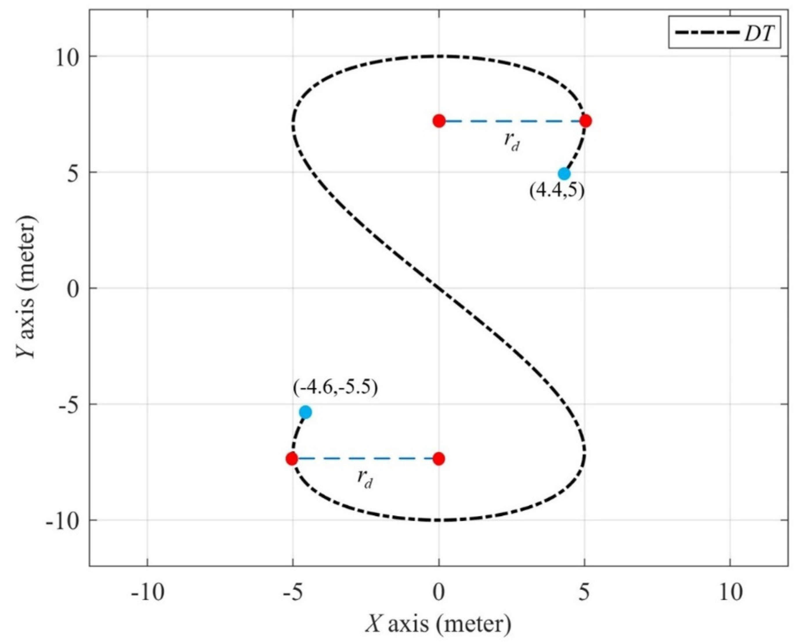
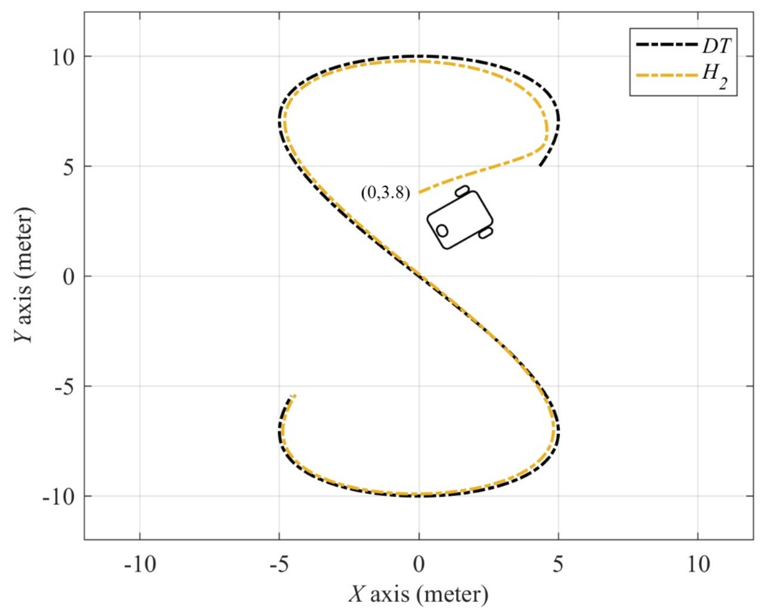
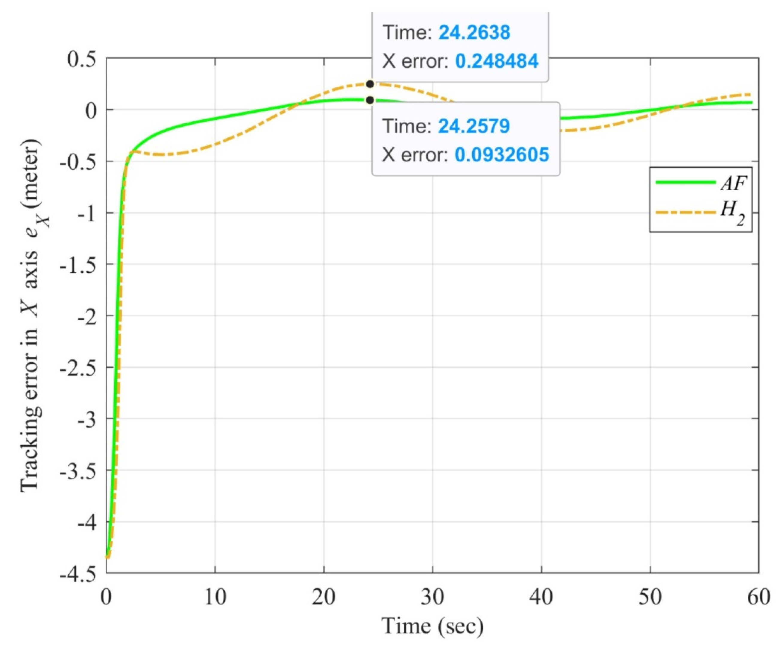
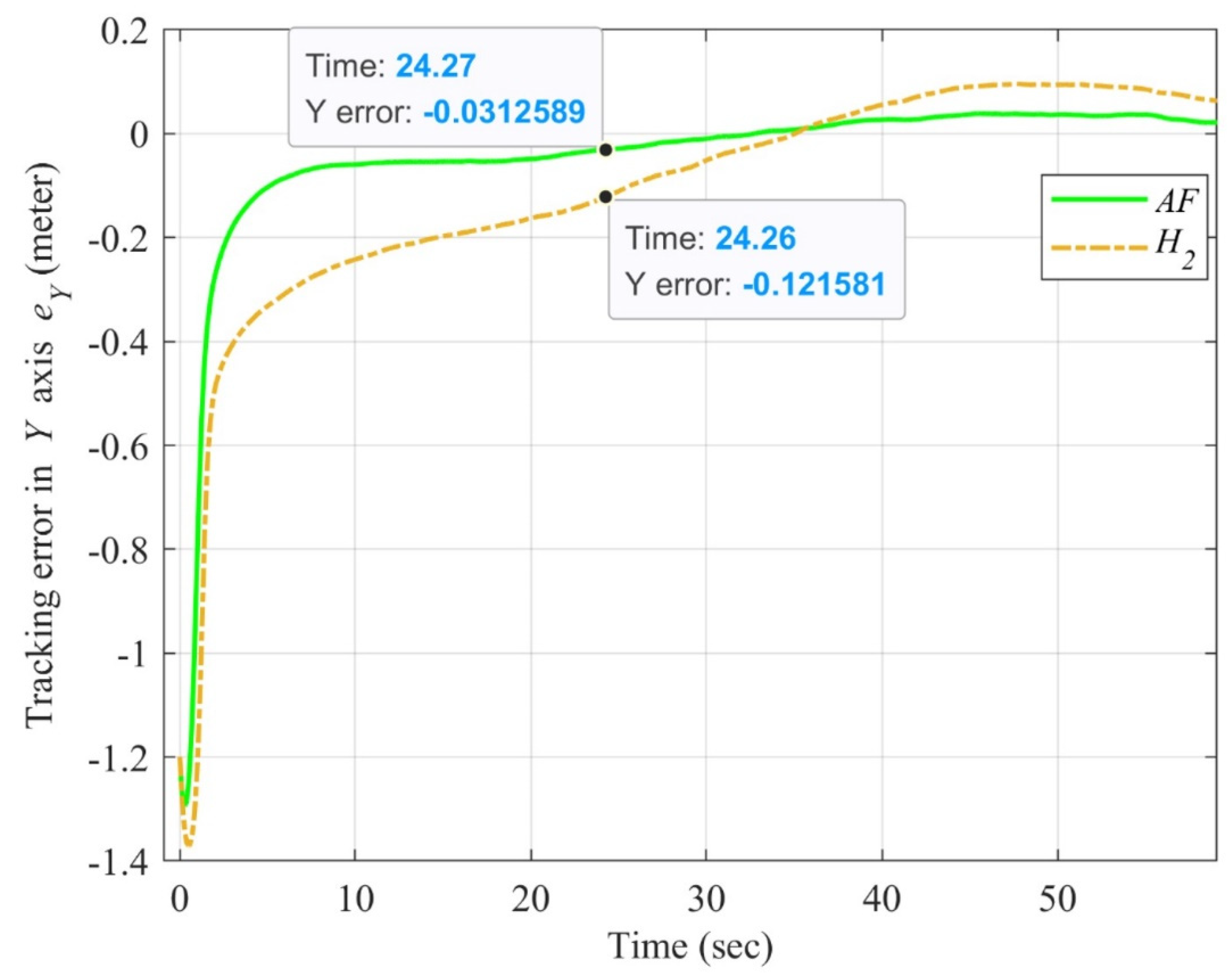
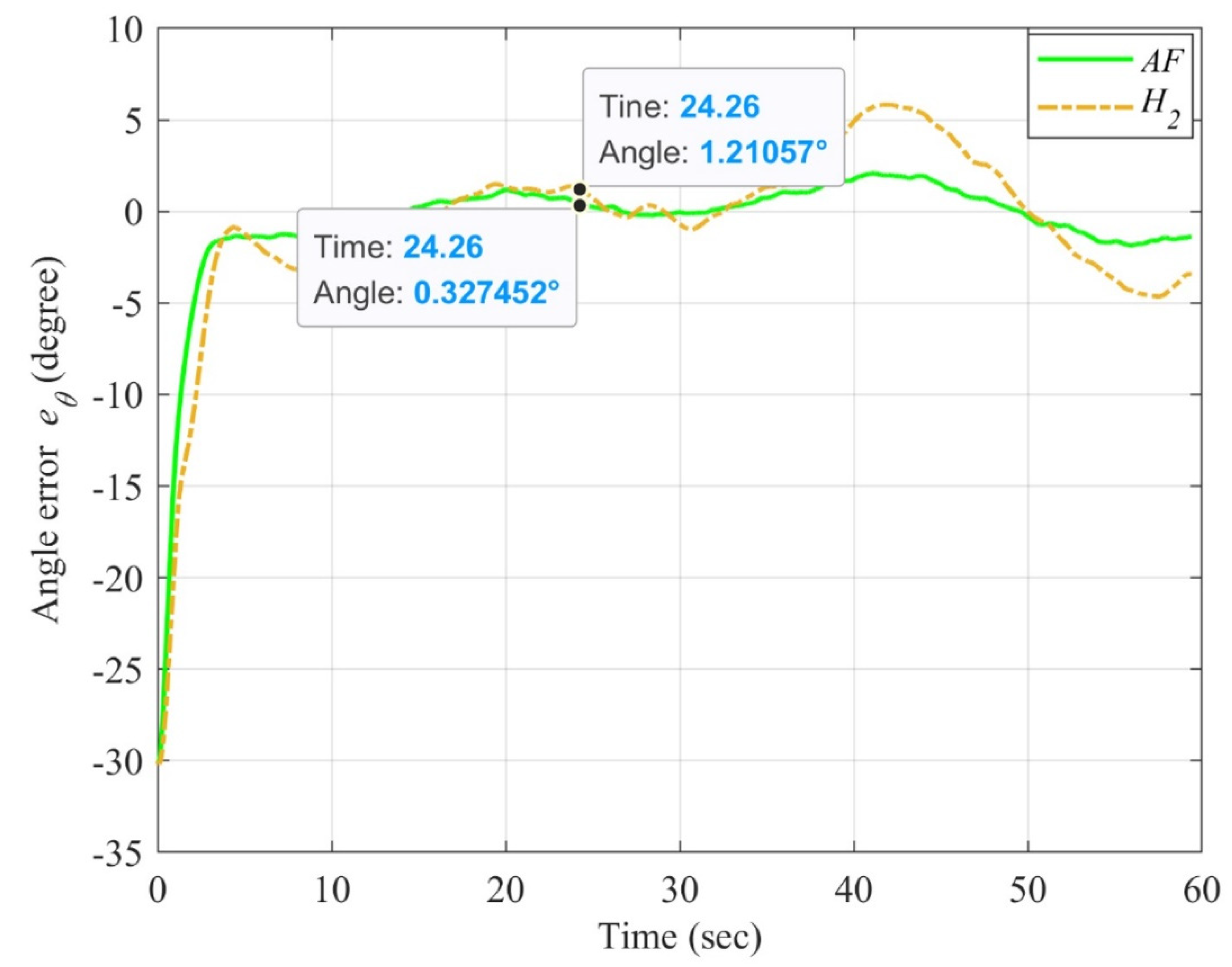
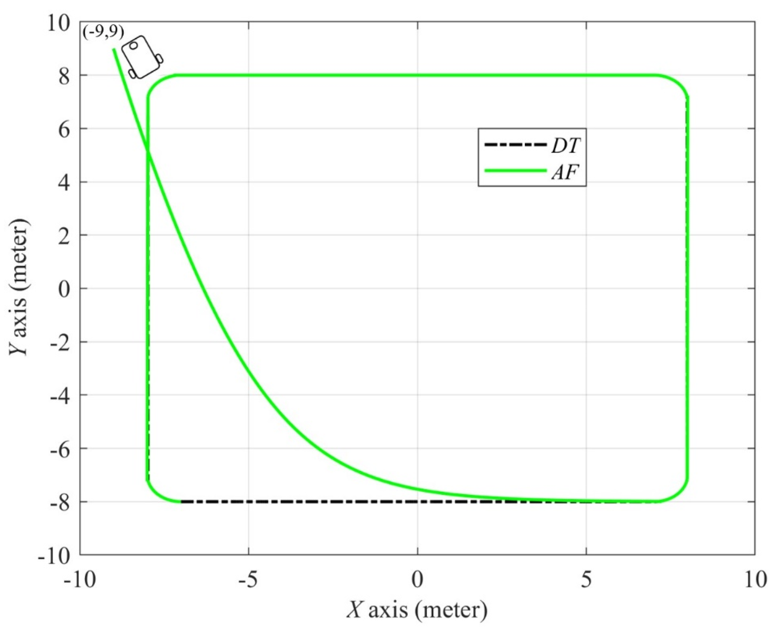
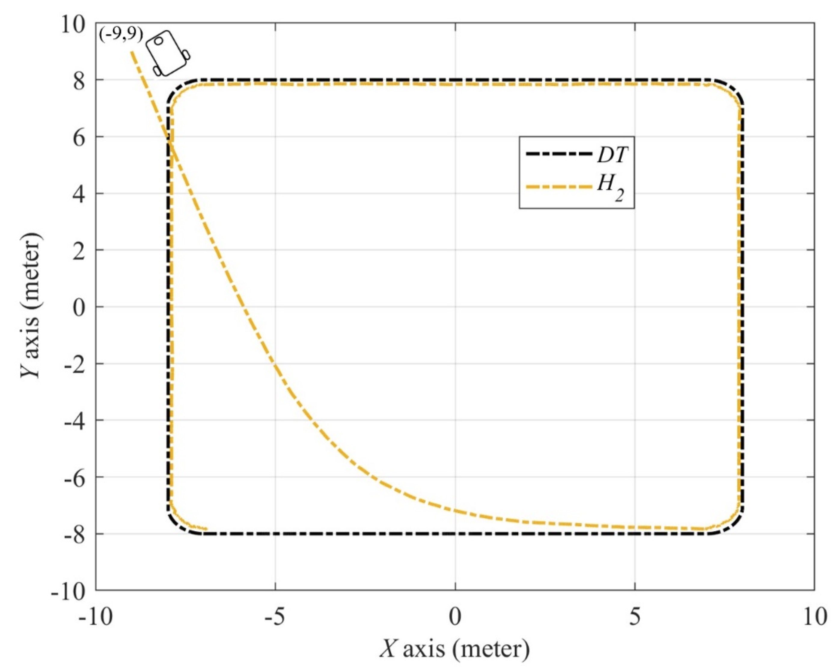
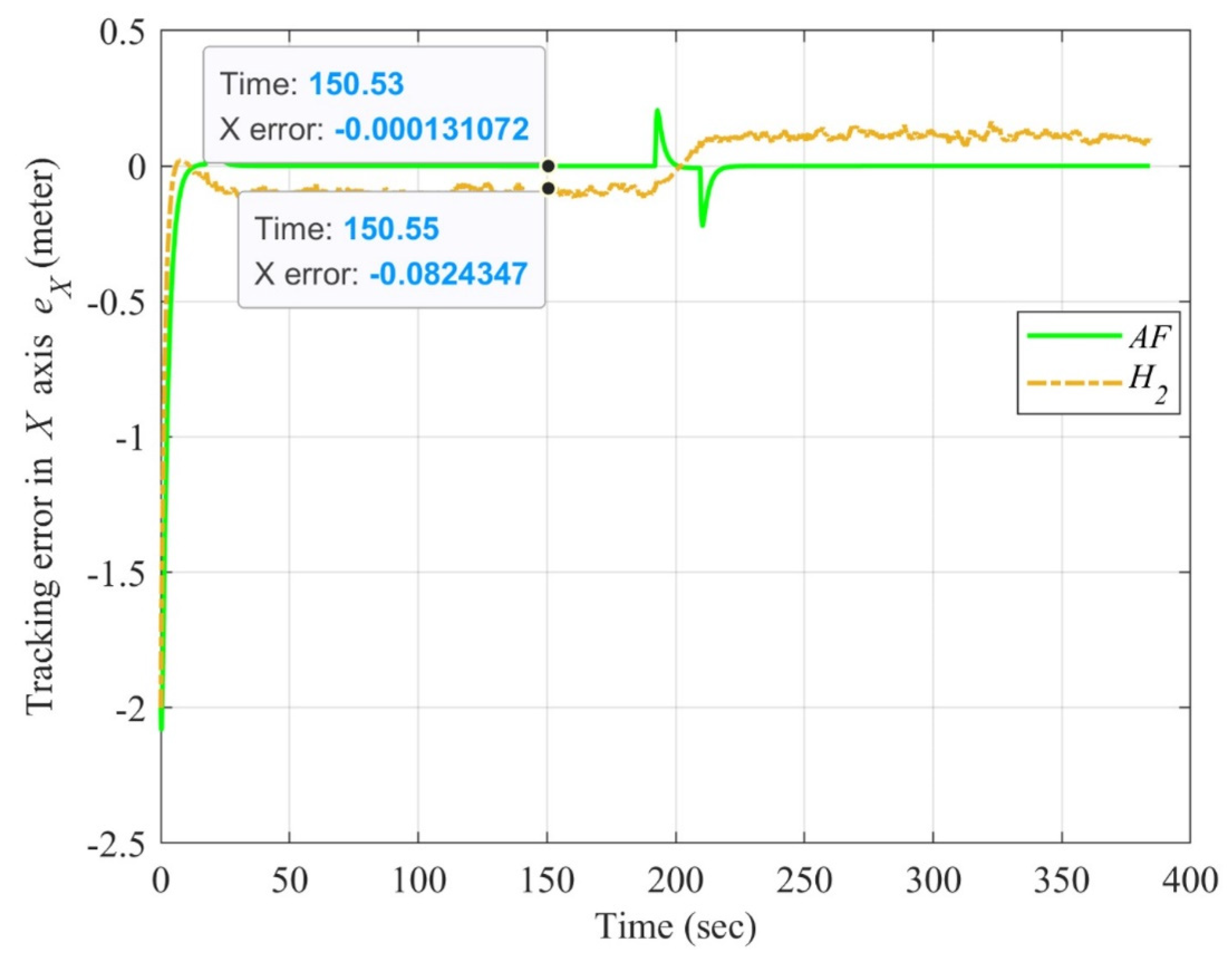
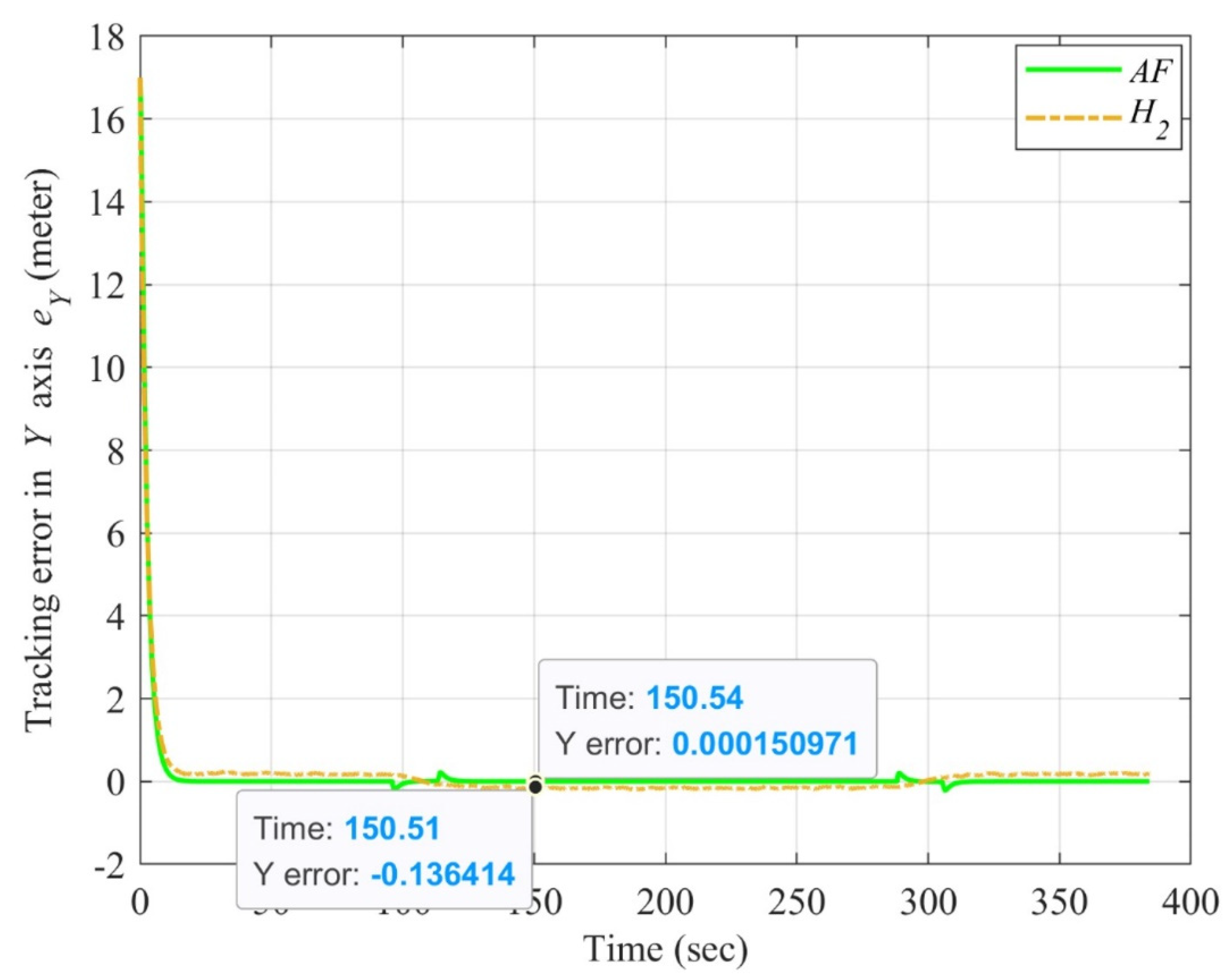
4.3. Simulation Results

As depicted above, a published H₂ control method is adopted in this investigation for comparison [24]. The system parameters of the WMR are provided in Table 1 and initial positions and attitude of the WMR are listed in Table 2. For explicitly presenting the simulation results of the S type and square trajectory, trajectory tracking results of this proposed adaptive fuzzy control method (AF) and the H₂ control method (H₂) with respect to the trajectory of the desired S type and square will be revealed separately in the following discussion.

The S type trajectory tracking results of the WMR controlled by using the adaptive fuzzy control method (AF) and H₂ control method (H₂) with initial conditions are shown in Figure 5 and Figure 6. From Figure 5 and Figure 6, the trajectory tracking performance can be found for this WMR in the first corner of the desired S type trajectory driven by these two control methods. Obviously, the WMR in Figure 5 controlled by the proposed adaptive fuzzy control method (AF) has quicker convergent rates in tracking the desired S type trajectory than the H₂ method (H₂) from the trajectory contour, even under the effect of a 20% modeling uncertainty of $\overline{m}$ which was not considered in the control design process of the H₂ control method.

The tracking errors in the X-axis, Y-axis and the heading angle of the WMR are illustrated in Figure 7, Figure 8 and Figure 9. The results depict the histories of tracking errors $e_X$,$e_Y$_, and $e_{\theta }$ for the WMR using the adaptive fuzzy control method and H₂ control method. From the comparisons of these tracking results, it is easy to see that the trajectory tracking performance of the H₂ control method is worse than the proposed adaptive fuzzy control method for the controlled WMR because of the existence of the effect of 20% modeling uncertainty caused by $\Delta m$. From these simulation results, both of these two control methods possess rapid transient response. However, larger tracking errors are found in the whole tracking period for the H₂ control method. On the whole, the proposed adaptive fuzzy control method obviously outperforms the H₂ control method in the WMR.

Figure 10 and Figure 11 reveal the square trajectory tracking results of the WMR driven by the adaptive fuzzy control method (AF) and H₂ method (H₂). The performance of the square trajectory tracking can be obtained for this WMR in four corners of the desired square trajectory driven by these two control methods. The WMR controlled by the proposed adaptive fuzzy control method (AF) demonstrated outstanding performance for tracking the desired square trajectory compared to the H₂ method (H₂) under the effect of a 20% modeling uncertainty of $\overline{m}$.

The tracking error results in the X-axis, Y-axis and the heading angle of the WMR can be found in Figure 12, Figure 13 and Figure 14. The results illustrate the performance of tracking errors $e_X$, $e_Y$, and $e_{\theta }$ for the desired square trajectory tracking of the WMR by adopting the adaptive fuzzy control method and H₂ control method. According to the compared results, it is obvious that the proposed adaptive fuzzy control method has a better trajectory tracking performance than the H₂ control method for the controlled WMR due to the $\Delta m$ effect of 20% modeling uncertainty. From these tracking error results, we can see that smaller tracking errors always can be obtained throughout the entire tracking period for the proposed adaptive fuzzy control method. On the whole, the H₂ control method is obviously inferior to the proposed adaptive fuzzy control method in the trajectory tracking of the WMR.

5. Conclusions

A nonlinear adaptive fuzzy control design with the skew symmetrical property is successfully developed for the trajectory tracking problem in wheeled mobile robots in this research. The main contribution of this study is the closed-form solution with adaptive fuzzy control method for the trajectory tracking problem in wheeled mobile robots. Based on the related literature, the closed-form solution for the trajectory tracking problem in wheeled mobile robots has still not been perfected due to the lack of optimal control methods for complex dynamics under modeling uncertainties. For achieving this investigative purpose, this study has several key contributions, i.e., the simplest and most easy-to-implement control structure for the trajectory tracking problem in wheeled mobile robots with a closed-form solution. According to the above results, this proposed method provides an energy consumption saving with complex control structures in practice. From the two simulation scenarios, the proposed adaptive fuzzy control method has better tracking performance of the desired S type and square trajectory than the H₂ method, no matter the convergence of tracking errors in X-axis, Y-axis and the heading angle, and in handling of modelling uncertainties.

References

1. Wang, C.; Liu, X.; Yang, X.; Hu, F.; Jiang, A.; Yang, C. Trajectory Tracking of an Omni-Directional Wheeled Mobile Robot Using a Model Predictive Control Strategy. Appl. Sci. 2018, 8, 231. [Google Scholar] [CrossRef] [Green Version]
2. Ullah, Z.; Xu, Z.; Lei, Z.; Zhang, L. A Robust Localization, Slip Estimation, and Compensation System for WMR in the Indoor Environments. Symmetry 2018, 11, 149. [Google Scholar] [CrossRef] [Green Version]
3. Li, Y.; Dai, S.; Zhao, L.; Yan, X.; Shi, Y. Topological Design Methods for Mecanum Wheel Configurations of an Omnidirectional Mobile Robot. Symmetry 2019, 11, 1268. [Google Scholar] [CrossRef] [Green Version]
4. Dosoftei, C.; Popovici, A.; Sacaleanu, P.; Gherghel, P.; Budaciu, C. Hardware in the Loop Topology for an Omnidirectional Mobile Robot Using Matlab in a Robot Operating System Environment. Symmetry 2021, 13, 969. [Google Scholar]
5. Eyad, A.; Mustafa, K. Modeling and Trajectory Planning Optimization for the Symmetrical Multi- Wheeled Omnidirectional Mobile Robot. Symmetry 2021, 13, 1033. [Google Scholar]
6. Chen, Y.H.; Chao, C.H.; Cheng, C.F.; Huang, C.J. A Fuzzy Control Design for the Trajectory Tracking of Autonomous Mobile Robot. Adv. Rob. Mech. Eng. 2020, 2, 206–211. [Google Scholar]
7. Nie, J.; Wang, Y.; Miao, Z.; Jiang, Y.; Zhong, H.; Lin, J. Adaptive Fuzzy Control of Mobile Robots with Full-State Constraints and Unknown Longitudinal Slipping. Non. Dyn. 2021, 106, 3315–3330. [Google Scholar] [CrossRef]
8. Du, O.; Sha, L.; Shi, W.; Sun, L. Adaptive Fuzzy Path Tracking Control for Mobile Robots with Unknown Control Direction. Discret. Dyn. Nat. Soc. 2021, 2021, 1–7. [Google Scholar] [CrossRef]
9. Brahim, M.; Hicham, A.; Mohammed, D. Fuzzy Adaptive Sliding Mode Controller for Electrically Driven Wheeled Mobile Robot for Trajectory Tracking Task. J. Con. Dec. 2022, 9, 71–79. [Google Scholar]
10. Amani, A.; Abderrazak, C. Indirect Neural Adaptive Control for Wheeled Mobile Robot. Int. J. Inn. Tech. Exp. Eng. 2019, 9, 2138–2145. [Google Scholar]
11. Chiraz, B.; Hassene, S. Design of a PID Optimized Neural Networks and PD Fuzzy Logic Controllers for a Two-Wheeled Mobile Robot. Asian J. Con. 2021, 23, 23–41. [Google Scholar]
12. Mateusz, S.; Marcin, S. Neural Tracking Control of a Four-Wheeled Mobile Robot with Mecanum Wheels. Appl. Sci. 2022, 12, 5322. [Google Scholar]
13. Zhai, J.Y.; Song, Z.B. Adaptive Sliding Mode Trajectory Tracking Control for Wheeled Mobile Robots. Int. J. Con. 2019, 92, 2255–2262. [Google Scholar] [CrossRef]
14. Krishanu, N.; Asifa, Y.; Anirban, N.; Manas, K.B. Event-Triggered Sliding-Mode Control of Two Wheeled Mobile Robot: An Experimental Validation. IEEE J. Emerg. Sel. Top. Ind. Elec. 2021, 2, 218–226. [Google Scholar]
15. Xie, Y.; Zhang, X.; Meng, W.; Zheng, S.; Jiang, L.; Meng, J.; Wang, S. Coupled Fractional-Order Sliding Mode Control and Obstacle Avoidance of a Four-Wheeled Steerable Mobile Robot. ISA Tran. 2021, 108, 282–294. [Google Scholar] [CrossRef]
16. Brahim, M.; Hicham, A.; Mohammed, D. Extended State Observer-Based Finite-Time Adaptive Sliding Mode Control for Wheeled Mobile Robot. J. Con. Dec. 2022, 9, 465–476. [Google Scholar]
17. Ibari, B.; Benchikh, L. Backstepping Approach for Autonomous Mobile Robot Trajectory Tracking. J. Elect. Eng. Comp. Sci. 2016, 2, 478–485. [Google Scholar]
18. Nasim, E.; Alireza, A.; Hossein, K. Balancing and Trajectory Tracking of Two-Wheeled Mobile Robot Using Backstepping Sliding Mode Control: Design and Experiments. J. Int. Rob. Sys. 2017, 87, 601–613. [Google Scholar]
19. Muhammad, J.R.; Attaullah, Y.M. Trajectory Tracking and Stabilization of Nonholonomic Wheeled Mobile Robot Using Recursive Integral Backstepping Control. Electronics 2021, 10, 1992. [Google Scholar]
20. Taniguchi, T.; Sugeno, M. Trajectory Tracking Controls for Non-Holonomic Systems Using Dynamic Feedback Linearization Based on Piecewise Multi-Linear Models. J. Appl. Math. 2017, 47, 1–13. [Google Scholar]
21. Korayem, M.H.; Yousefzadeh, M.; Manteghi, S. Dynamics and Input–Output Feedback Linearization Control of a Wheeled Mobile Cable-Driven Parallel Robot. Mult. Sys. Dyn. 2017, 40, 55–73. [Google Scholar] [CrossRef]
22. Welid, B.; Rabah, M.; Mohammed, S.B. The Impact of the Dynamic Model in Feedback Linearization Trajectory Tracking of a Mobile Robot. Period. Pol. Elec. Eng. Comp. Sci. 2021, 65, 329–343. [Google Scholar]
23. Chen, Y.H.; Li, T.H.S.; Chen, Y.Y. A Novel Nonlinear Control Law with Trajectory Tracking Capability for Mobile Robots: Closed-Form Solution Design. Appl. Math. Inf. Sci. 2013, 7, 749–754. [Google Scholar] [CrossRef]
24. Chen, Y.H.; Chen, Y.Y.; Lou, S.J.; Huang, C.J. Energy Saving Control Approach for Trajectory Tracking of Autonomous Mobile Robots. Intel. Auto. Soft Comp. 2021, 30, 1–17. [Google Scholar] [CrossRef]
25. Chen, Y.H.; Lou, S.J. Control Design of a Swarm of Intelligent Robots: A Closed-Form H2 Nonlinear Control Approach. Appl. Sci. 2020, 10, 1055. [Google Scholar] [CrossRef] [Green Version]
26. Chen, Y.H.; Chen, Y.Y. Trajectory Tracking Design for a Swarm of Autonomous Mobile Robots: A Nonlinear Adaptive Optimal Approach. Mathematics 2022, 10, 3901. [Google Scholar] [CrossRef]
27. Kasra, E.; Farzaneh, A.; Heidar, A.T. Adaptive Control of Uncertain Nonaffine Nonlinear Systems with Input Saturation Using Neural Networks. IEEE Tran. Neu. Net. Lear. Sys. 2015, 26, 2311–2322. [Google Scholar]
28. Aguiar, A.P.; Hespanha, J.P. Trajectory-Tracking and Path-Following of Underactuated Autonomous Vehicles with Parametric Modeling Uncertainty. IEEE Tran. Auto. Cont. 2007, 52, 1362–1379. [Google Scholar] [CrossRef] [Green Version]
29. Shen, M.; Wu, X.; Park, J.H.; Yi, Y.; Sun, Y. Iterative Learning Control of Constrained Systems with Varying Trial Lengths Under Alignment Condition. IEEE Tran. Neu. Net. Lear. Syst. 2021, 1–7. Available online: https://ieeexplore.ieee.org/document/9664474 (accessed on 21 December 2022). [CrossRef]
30. Shen, M.; Wang, X.; Park, J.H.; Yi, Y.; Che, W.W. Extended Disturbance-Observer-Based Data-Driven Control of Networked Nonlinear Systems with Event-Triggered Output. IEEE Tran. Sys. Man Cyb. 2022, 1–12. Available online: https://ieeexplore.ieee.org/document/9966320 (accessed on 21 December 2022). [CrossRef]
31. Das, T.; Kar, I.N.; Chaudhury, S. Simple Neuron-Based Adaptive Controller for a Nonholonomic Mobile Robot Including Actuator Dynamics. Neurocomputing 2006, 69, 2140–2151. [Google Scholar] [CrossRef]
32. Boukens, M.; Boukabou, A. Design of an Intelligent Optimal Neural Network-Based Tracking Controller for Nonholonomic Mobile Robot Systems. Neurocomputing 2017, 226, 46–57. [Google Scholar] [CrossRef]
33. Chen, B.S.; Chang, Y.C. Nonlinear Mixed H2/H ∞ Control for Robust Tracking Design of Robotic Systems. Int. J. Cont. 1997, 67, 837–857. [Google Scholar] [CrossRef]
Figure 1. Wheeled mobile robot dynamic system.
Symmetry 15 00221 g001
Figure 2. The closed-loop control diagram of a WMR via the proposed method.
Symmetry 15 00221 g002
Figure 3. The desired S type trajectory with a radius of 5 m from x0 = 0 m, y0 = 0 m.
Symmetry 15 00221 g003
Figure 4. The desired square trajectory with a radius of 8 m from x0 = −7 m, y0 = −8 m.
Symmetry 15 00221 g004
Figure 5. The result of the S type trajectory by the adaptive fuzzy control method from x = 0 m, y = 3.8 m.
Symmetry 15 00221 g005
Figure 6. The result of the S type trajectory by the H2 control method from x = 0 m, y = 3.8 m.
Symmetry 15 00221 g006
Figure 7. The X axis errors of the adaptive fuzzy and H2 control method for S type trajectory from x = 0 m, y = 3.8 m.
Symmetry 15 00221 g007
Figure 8. The Y axis errors of the adaptive fuzzy and H2 control method for S type trajectory from x = 0 m, y = 3.8 m.
Symmetry 15 00221 g008
Figure 9. The angle errors of the adaptive fuzzy and H2 control method for S type trajectory from x = 0 m, y = 3.8 m.
Symmetry 15 00221 g009
Figure 10. The result of the square trajectory by the adaptive fuzzy control method from x = −9 m, y = 9 m.
Symmetry 15 00221 g010
Figure 11. The result of the square trajectory by the H2 control method from x = −9 m, y = 9 m.
Symmetry 15 00221 g011
Figure 12. The X axis errors of the adaptive fuzzy and H2 control method for the square trajectory from x = −9 m, y = 9 m.
Symmetry 15 00221 g012
Figure 13. The Y axis errors of the adaptive fuzzy and H2 control method for square trajectory from x = −9 m, y = 9 m.
Symmetry 15 00221 g013
Figure 14. The angle errors of the adaptive fuzzy and H2 control method for the square trajectory from x = −9 m, y = 9 m.
Symmetry 15 00221 g014