Optimization of Software Test Scheduling under Development of Modular Software Systems

Abstract

Software testing and debugging is a crucial part of the software development process since defective software not only incurs customer dissatisfaction but also might incur legal issues. However, the managers of a software development company cannot arbitrarily prolong their software debugging period due to their software testing budget and opportunity in the market. Accordingly, in order to propose an advantageous testing project, the managers should be aware of the influence of the testing project on cost, quality, and time to make the best decision. In this study, a new software reliability growth model (SRGM) with consideration of the testing staff’s learning effect is proposed to achieve better prediction. The methods of estimating the model’s parameters and the symmetric confidence intervals are also proposed in the study. Moreover, in the past, most of the SRGMs focused on a single software system. However, in practice, some software systems were developed using modular-based system engineering approaches. Therefore, traditional software testing work can be changed to multiple modular testing work in this scenario. Therefore, the manager can use this to dispatch multiple staff groups to perform the individual testing work simultaneously. The study proposes two mathematical programming models to handle the scheduling of modular testing work. Additionally, the design of a computerized decision support system is also proposed in the study for the application in practice.

1. Introduction

Nowadays, software reliability has always been one of the most critical indicators for evaluating the quality of software, and this information can be used to make an appropriate plan for software testing for ensuring the software quality remains high. There is no doubt that the modern software industry focuses on the functionality of software, but also ensures that the quality and stability of software must be above an acceptable level as well. In other words, no matter how superior the performance and functionality of the software are, if the quality and stability of the software cannot satisfy their customers or clients’ requirements, this still leads to sales losses. Nevertheless, due to the constraints of the testing project’s budget, manpower, and testing time, it would be unrealistic to expect software developers to strive for perfect and faultless software in order to successfully complete the project. As a result, rather than spending a large budget pursuing a flawless software system, most of the software developers would make a compromised testing plan. There have been many software reliability growth models (SRGMs) proposed over the past few decades, and most of them were based on a Non-Homogeneous Poisson Process (NHPP) in order to describe software testing and debugging phenomena [1,2,3,4,5,6,7,8,9,10,11,12,13,14,15,16,17,18,19,20].

In the past decades, classic SRGMs have been classified into two types (concave and S-type), and the S-type SGRMs can identify the phenomenon of testing the learning process of the staff. This means that as the testing staff becomes more familiar with the software and test tools, their debugging ability and test efficiency will increase incrementally. The study by Xia et al. [21] is an early attempt to investigate the influence of learning on software reliability growth, and their hypothesis is that the learning effect can simply be attributed to the experience of the testing staff. Furthermore, according to Chatterjee et al. [22], testing efforts and learning factors can be combined in a model that can effectively reflect the growing process of software reliability. Similarly, Kapur et al. [23] have proposed a related model based on a similar idea, where testing effort as a logistic function is explained as the effect of testing effort. In contrast to exponential and S-shaped models, Chiu et al. [24] developed an NHPP-based SRGM that shows a better fitness with software faults data than the previous models. Kapur et al. [25] adopted a control theoretical method in order to determine the dynamic allocation of optimal testing effort under various scenarios. They considered that the experience of the learning effect will make an inference on the testing effort. Duffey and Fiondella [26] investigated whether learning trends exist in software testing or not. They concluded that it may not be evident in all the testing data. In contrast, if there exists a learning effect in testing projects, their model can estimate the learning performance from the experience and skill of the testing staff. Fang and Yeh [27] proposed confidence interval estimation of a learning effect model under NHPP-based assumptions. Zhu and Pham [28] have concluded that in order to increase the reliability of software development, the testing environment is the most important factor to consider. They considered that an individual’s domain knowledge and education can have a significant impact on the effectiveness of a software testing project. There have been several experiments done by Lemos et al. [29] to see what the effect of testing experience and knowledge have on software reliability. Chiu et al. [30] proposed a learning-based SRGM with linear or exponential growth with testing time. As a result, their extended model can also be used to describe the phenomenon of unstable debugging efficiency during the early stages of software development. Lee et al. [31] proposed enhancing software reliability by utilizing a sequential probability ratio test. It would be more efficient than most classic models based on NHPP. Tian et al. [32,33] proposed two software reliability growth models, and their models not only measured human learning factors but also considered human negligence factors. Furthermore, their model can be applied in dealing with software reliability prediction under insufficient historical testing data. Chang et al. [34] utilized a classic software reliability model with a learning effect to develop a more reliable estimation of statistical confidence intervals. Huang et al. [35] further assumed that the learning effect is time-dependent and may have error fluctuation over time to construct an NHPP-based SRGM for fitting with S-shaped and exponential software testing data. According to the above discussion, it is important to note that, although the learning effect has been taken into consideration in the previous studies, their works did not give a clear learning parameter for measuring the effect. In this study, we have solved the issue by designing two parameters (learning factor and autonomous errors-detected factor) to measure the testing staff’s learning effect.

In a modular software system environment, the whole system can be decomposed into several modules, and therefore the testing work can also be dispatched to different testing teams. This will speed up the testing process. Some studies began to focus on how to schedule the testing work. They developed mathematical programming models and heuristic algorithms for dealing with software test scheduling. Coit and Smith [36] developed a genetic algorithm to solve the reliability issue of series-parallel systems. They designed a dynamic penalty function, and claimed that their solution approach could solve a dual of nonlinear optimization problem. Dai et al. [37] also proposed a genetic algorithm for allocating testing-resources for modular software systems. Their model has considered how to achieve the objectives of minimizing testing cost and maximizing system reliability. Levitin [38] proposed a heuristic algorithm to evaluate the expected execution time and the corresponding reliability for modular hardware or software systems. However, Levitin’s proposed reliability model does not belong to the SRGM because the reliability of the model cannot be grown with testing time. Such a model can only apply in some specific areas, and it is not easy to extend to some software testing projects. Kang et al. [39] proposed an approach for implementing modular adaptation of scientific software. As a result, they take adaptability into account separately in software development and enable one to design scientific programs in a separate manner. Wang and Ma [40] developed a hybrid particle swarm optimization to solve industrial complex reliability problems with implicit performance functions and correlated non-normal variables. Their proposed model was applied to a hydropower station’s reliability issue with consideration of practical engineering experience and the particular geological and mechanical parameters present at the site, allowing them to deal with the reliability effectively. Serban and Shaikh [41] proposed a new approach to predict software reliability by using package-level modularization metrics. The study focused on the empirical experimentation of relevant fault severity information with package level metrics in an effort-aware classification and ranking scenario based on fault severity. Chunyan et al. [42] proposed a Bayesian support vector machine for solving the design of modular systems with consideration of software reliability. The study seeks to mitigate the computational effort involved in this process as effectively as possible. Additionally, some studies examined how to assign and schedule software testing tasks in order to achieve the highest level of reliability in modular software environments with complex relationships, such as software modules running in parallel and serial.

Our study provides the following contributions based on the above discussion and which are different from what is already available in the literature in the field: (1) The other SRGMs’ parameters are less meaningful and intuitive, so domain engineers or experts are not easily able to evaluate them. However, our proposed SRGM’s parameters are originated from human factors with the learning effect, and they would be easily estimated and explained. Accordingly, it would be easy to apply in different scenarios. (2) Most of the related studies regarding software release decisions only focused on a single software system and did not consider the constraints of testing time, resources, and reliability. Therefore, there was significantly less discussion on how to arrange the testing schedule under a modular software system development. In this study, the proposed programming models can arrange the testing resources among all software subsystems and corresponding modules under predefined constraints. It can effectively shorten a software testing period under a reasonable cost. (3) The study provides the managerial insights and suggestions for software developers to make a better software release decision. In addition, the reasonable estimation of statistical confidence intervals for individual parameters and the mean value function is also proposed in this study. Our study would be helpful to the software developers to manage any possible situations in a testing period because most related studies overly focused on prediction accuracy instead of possible ranges of estimation.

As for the rest of this paper, it is organized in the following manner: Section 2 discusses the development of the basic model with the learning effect, parameter estimation, and the verification of the fitting ability of the model. Section 3 provides the decision models for a single software system and modular software system. The design of a computerized decision support system is also introduced in this section. Section 4 presents the application and numerical analysis. Finally, Section 5 gives the conclusion and future works.

2. Mathematical Development of Software Reliability Growth Model

2.1. Basic Model Development

Software Reliability Growth Models (SRGMs) can be used to estimate and forecast the expected number of failures under different testing/debugging periods, and they also give an indicator for measuring the software quality and reliability when it is released. Over the course of the past few decades, more than a dozen different software reliability models have been presented. The many stages of the software development life cycle served as the foundation for these models. Generally, classic SRGMs can be categorized into two types (Concave, S-shaped). However, the fact that most of the previously created models can only be used to fit Concave or S-type testing data, neither of which can be interpreted in a meaningful way, is one of the problems with those models. As a result of testing staff members’ learning processes, the S-shaped SRGM can be explained. It means that testing staff will get better at finding bugs and testing faster as they learn more about the software and test tools. Based on the above-mentioned information, a new SRGM is developed to fit Concave or S-shaped testing data with consideration of testing staff members’ learning processes in this study.

It is assumed that the occurrence of software defects (errors) follows an NHPP and that any recognized defects will be eliminated instantly. Therefore, the correcting time for a software defect can therefore be negligible. Moreover, the notion of learning effect is examined in order to construct an effective model for forecasting software reliability. In this study, there are two critical factors are considered. One is the autonomous error detection factor (${\alpha }_p$), which can represent a testing staff’s basic ability from past training and knowledge. Another is the learning factor (${\beta }_p$), which can represent a testing staff’s learning from reviewing various error patterns during a software testing phase. In the scenario of modular software development, the number of potential errors was hidden in the $j$th subsystem ($a_j$), which can be evaluated by an error-seeding method. Suppose the average number of detected errors can be estimated by the mean value function $M\left(T_j,a_j,{\alpha }_p,{\beta }_p\right)$. Therefore, after a software testing period $T_j$, the number of undetected software errors will be decreased to $a_j-M\left(T_j,a_j,{\alpha }_p,{\beta }_p\right)$. However, the equation form of $M\left(T_j,a_j,{\alpha }_p,{\beta }_p\right)$ would be required to infer this. Due to the fact that ${\alpha }_p$ is a major factor in influencing the velocity of errors detection, the manager should pay more attention to this to assign appropriate testing work to individual staff groups. Furthermore, ${\beta }_p$ also influences software errors detection, but its influence degree is subject to the number of errors detected previously. Generally, the number of errors detected under a testing time can be defined as the mean value function, and therefore the velocity of software error detection will be ${\beta }_{p}M\left(T_j,a_j,{\alpha }_p,{\beta }_p\right)/a_j$. This indicates that it will be beneficial to identify new software errors in the future if more errors have been found in the past. Based on the above mentioned, the definition of the detection rate can be used to model the relationships among the two critical factors and the mean value function as follows:

$$D\left(T_j\right)=\frac{dM\left(T_j,a_j,{\alpha }_p,{\beta }_p\right)/d{T}_j)}{a_j-M\left(T_j,a_j,{\alpha }_p,{\beta }_p\right)}={\alpha }_p+{\beta }_p\left(\frac{M\left(T_j,a_j,{\alpha }_p,{\beta }_p\right)}{a_j}\right)$$

(1)

The error detection rate function $D\left(T_j\right)$ can be used to investigate the variation in the proportion of errors detected at time $T_j$. In order to obtain the mathematical form of the mean value function $M\left(T_j,a_j,{\alpha }_p,{\beta }_p\right)$, Equation (1) can be arranged as follows:

$$⟹\frac{dM\left(T_j,a_j,{\alpha }_p,{\beta }_p\right)}{d{T}_j}=\left(a_j-M\left(T_j,a_j,{\alpha }_p,{\beta }_p\right)\right)\left({\alpha }_p+\left(\frac{{\beta }_p}{a_j}\right)M\left(T_j,a_j,{\alpha }_p,{\beta }_p\right)\right)$$

(2)

In Equation (2), it can be seen that the number of errors detected per time can be transformed into a quadratic form. In order to apply a differential equation in Equation (2), we need to preprocess it as follows:

$$⟹\frac{dM\left(T_j,a_j,{\alpha }_p,{\beta }_p\right)/d{T}_j}{\left(a_j-M\left(T_j,a_j,{\alpha }_p,{\beta }_p\right)\right)\left({\alpha }_p+\left(\frac{{\beta }_p}{a_j}\right)M\left(T_j,a_j,{\alpha }_p,{\beta }_p\right)\right)}=1.$$

(3)

To take the integral of both sides, the following result can be obtained as follows:

$$⟹\int \frac{dM\left(T_j,a_j,{\alpha }_p,{\beta }_p\right)/d{T}_j}{\left(a_j-M\left(T_j,a_j,{\alpha }_p,{\beta }_p\right)\right)\left({\alpha }_p+\left(\frac{{\beta }_p}{a_j}\right)M\left(T_j,a_j,{\alpha }_p,{\beta }_p\right)\right)}d{T}_j=\int 1d{T}_j.$$

(4)

To the left of Equation (4), the integral variable $T_j$ can be changed into $M\left(T_j,a_j,{\alpha }_p,{\beta }_p\right)$ as follows:

$$⟹\int \frac{-\left(\frac{a_j}{{\beta }_p}\right)}{\left(M\left(T_j,a_j,{\alpha }_p,{\beta }_p\right)-a_j\right)\left(M\left(T_j,a_j,{\alpha }_p,{\beta }_p\right)+a_j\left(\frac{{\alpha }_p}{{\beta }_p}\right)\right)}dM\left(T_j,a_j,{\alpha }_p,{\beta }_p\right)=T_j+constant.$$

(5)

In order to get the integration of the left side smoothly, the fraction needs to be divided into the two parts as follows:

$$⟹\left(\frac{-1}{{\alpha }_p+{\beta }_p}\right)\int \left[\frac{dM\left(T_j,a_j,{\alpha }_p,{\beta }_p\right)}{M\left(T_j,a_j,{\alpha }_p,{\beta }_p\right)+a_j\left(\frac{{\alpha }_p}{{\beta }_p}\right)}-\frac{dM\left(T_j,a_j,{\alpha }_p,{\beta }_p\right)}{M\left(T_j,a_j,{\alpha }_p,{\beta }_p\right)-a_j}\right]=T_j+constant.$$

(6)

After integrating the left side of Equation (6), we can obtain the mathematical form regarding log functions as follows:

$$⟹\left(\frac{-1}{{\alpha }_p+{\beta }_p}\right)\left(\ln \left[M\left(T_j,a_j,{\alpha }_p,{\beta }_p\right)+\frac{a_j{\alpha }_p}{{\beta }_p}\right]-\ln \left[M(T_j,a_j | {\alpha }_p,{\beta }_p)-a_j\right]\right)=T_j+constant$$

(7)

By combining the two log functions, we can alter it concisely.

$$⟹\ln \left[\frac{M\left(T_j,a_j,{\alpha }_p,{\beta }_p\right)+a_j\left(\frac{{\alpha }_p}{{\beta }_p}\right)}{M\left(T_j,a_j,{\alpha }_p,{\beta }_p\right)-a_j}\right]=-\left({\alpha }_p+{\beta }_p\right)\left(T_j+constant\right).$$

(8)

Taking the exponential of both sides, the logarithm on the left side can be eliminated as follows:

$$⟹\frac{M\left(T_j,a_j,{\alpha }_p,{\beta }_p\right)+a_j\left(\frac{{\alpha }_p}{{\beta }_p}\right)}{M\left(T_j,a_j,{\alpha }_p,{\beta }_p\right)-a_j}=e^{-\left({\alpha }_p+{\beta }_p\right)\left(T_j+constant\right)}$$

(9)

Solving Equation (9) for $M\left(T_j,a_j,{\alpha }_p,{\beta }_p\right)$, the mathematical form of $M\left(T_j,a_j,{\alpha }_p,{\beta }_p\right)$ with the unknown constant is as follows:

$$M\left(T_j,a_j,{\alpha }_p,{\beta }_p\right)=\frac{a_j\left({\alpha }_p+e^{\left({\alpha }_p+{\beta }_p\right)\left(T_j+constant\right)}\right)}{e^{\left({\alpha }_p+{\beta }_p\right)\left(T_j+constant\right)}-{\beta }_p}.$$

(10)

The initial condition $M\left(T_j=0,a_j, {\alpha }_p,{\beta }_p\right)=0$ is given (no software error or fault detected at testing time $T_j=0$), and therefore we can utilize it for obtaining the unknown constant value as follows:

$$M\left(T_j=0,a_j, {\alpha }_p,{\beta }_p\right)=\frac{a_j\left({\alpha }_p+e^{\left({\alpha }_p+{\beta }_p\right)\left(constant\right)}\right)}{e^{\left({\alpha }_p+{\beta }_p\right)\left(constant\right)}-{\beta }_p}=0.$$

(11)

Solving Equation (11) for the unknown constant, the value of the constant will be as follows:

$$constant=\frac{ln\left[-{\alpha }_p\right]}{{\alpha }_p+{\beta }_p}.$$

(12)

Substituting the constant into Equation (10), the complete form of the mean value function $M\left(T_j,a_j,{\alpha }_p,{\beta }_p\right)$ can be obtained as follows:

$$M\left(T_j,a_j,{\alpha }_p,{\beta }_p\right)=\frac{a_j{\alpha }_p\left(e^{\left({\alpha }_p+{\beta }_p\right)T_j}-1\right)}{{\alpha }_p{e}^{\left({\alpha }_p+{\beta }_p\right)T_j}+{\beta }_p}.$$

(13)

Furthermore, the intensity function $\lambda \left(T_j,a_j,{\alpha }_p,{\beta }_p\right)$ (the number of the errors detected at time $t$) can be obtained as follows:

$$\lambda \left(T_j,a_j,{\alpha }_p,{\beta }_p\right)=\frac{dM\left(T_j,a_j,{\alpha }_p,{\beta }_p\right)}{d{T}_j}=a_j{e}^{\left({\alpha }_p+{\beta }_p\right)T_j}{\left(\frac{{\alpha }_p+{\beta }_p}{{\alpha }_p{e}^{\left({\alpha }_p+{\beta }_p\right)T_j}+{\beta }_p}\right)}^2.$$

(14)

If the software manager wants to evaluate the efficiency of testing and debugging, the error detection rate is helpful as the indicator. Equation (1) has given a simple form for it; however, we can use Equation (13) to obtain the complete form of $D\left(T_j\right)$ as follows:

$$D\left(T_j\right)=\frac{dM\left(T_j,a_j,{\alpha }_p,{\beta }_p\right)/d{T}_j)}{a_j-M\left(T_j,a_j,{\alpha }_p,{\beta }_p\right)}=\frac{{\alpha }_p\left({\alpha }_p+{\beta }_p\right){\mathrm{e}}^{\left({\alpha }_p+{\beta }_p\right)T_j}}{{\beta }_p+{\alpha }_p{\mathrm{e}}^{\left({\alpha }_p+{\beta }_p\right)T_j}}.$$

(15)

According to the above mentioned, a Counting function can be used to describe the process of software reliability growth. $\left\{N\left(T_j\right),t\ge 0\right\}$, where$N\left(T_j\right)$ follows an NHPP with the mean value function $M\left(T_j,a_j,{\alpha }_p,{\beta }_p\right)$, and the probability can be formulated as follows:

$$\mathrm{Pr}\left(N\left(T_j\right)=k\right)=\frac{{\left[M\left(T_j,a_j,{\alpha }_p,{\beta }_p\right)\right]}^k{e}^{-M\left(T_j,a_j,{\alpha }_p,{\beta }_p\right)}}{k!}, k=0,1,2,\dots$$

(16)

However, the total number of undetected errors will affect the software reliability, which will increase the software risk. Accordingly, the software reliability needs to be evaluated, and it can be calculated as follows:

$$R\left(x|T_j,a_j,{\alpha }_p,{\beta }_p\right)=e^{-\left(M\left(T_j+x,a_j, {\alpha }_p,{\beta }_p\right)-M\left(T_j,a_j, {\alpha }_p,{\beta }_p\right)\right)}.$$

(17)

Decision makers can give an adequate value of operating time $x$ for managerial requirements in order to maintain stability in practice. There is no doubt that increasing the operating time will have a negative impact on the reliability of the system. It is also worth mentioning that as the testing time approaches infinity, the software reliability will finally approach one ($\underset{t\to \infty }{\lim }R\left(x|T_j,a_j,{\alpha }_p,{\beta }_p\right)\to 1$).

2.2. Estimation of Parameters and Confidence Intervals

The model parameters in this study can be estimated by using any of the two estimating techniques. Gathered data on software failures are used to illustrate how well the suggested model fits with other ones that are already in use.

(1) Least-squares estimation (LSE) is one of the most commonly used methods in statistics for estimating the parameters of models by minimizing the sum of the squares of the residuals. There is a set of pairs of observed data that are taken into account in this analysis, i.e., $\left\{\left(T_j^{\left(0\right)},M^{\left(0\right)}\right),\left(T_j^{\left(1\right)},M^{\left(1\right)}\right),\left(T_j^{\left(2\right)},M^{\left(2\right)}\right),\dots ,\left(T_j^{\left(n\right)},M^{\left(n\right)}\right)\right\}$, to estimate all parameters of the proposed model. Here, $M^{\left(i\right)}$ is the actual number of errors detected within the period [$0,T_j^{\left(n\right)}]$, and this calculation can be presented by the following:

$$\mathrm{Min}ER\left(a_j,{\alpha }_p,{\beta }_p\right)={\displaystyle \sum }_{i=1}^n{\left(M^{\left(i\right)}-M\left(T_j^{\left(i\right)},a_j, {\alpha }_p,{\beta }_p\right)\right)}^2$$

(18)

It is necessary to take the first-order derivative of Equation (18) with respect to the parameters $a_j, {\alpha }_p,{\beta }_p$ of the model for minimizing the sum of the squares of the residuals. Furthermore, letting them be equal to zero, the simultaneous equations can be given as follows:

$$\frac{\partial ER\left(a_j,{\alpha }_p,{\beta }_p\right)}{\partial a_j}=\frac{\partial ER\left(a_j,{\alpha }_p,{\beta }_p\right)}{\partial {\alpha }_p}=\frac{\partial ER\left(a_j,{\alpha }_p,{\beta }_p\right)}{\partial {\beta }_p}=0.$$

(19)

In order to obtain the estimated parameter values for the simultaneous equations, numerical methods are employed as they are unable to provide a closed-form expression of the solution. Software testing managers, however, can simplify the estimation of the remaining parameters by solving the simultaneous equations $\frac{\partial ER\left({\overline{a}}_j,{\alpha }_p,{\beta }_p\right)}{\partial {\alpha }_p}=\frac{\partial ER\left({\overline{a}}_j,{\alpha }_p,{\beta }_p\right)}{\partial {\beta }_p}=0$ if they estimate the parameter ${\overline{a}}_j$ by using an error seeding method based on the system scale for the parameters’ estimation.

(2) Maximum Likelihood Estimation method (MLE) is another way to estimate the probability distribution’s parameters. Since the operation follows a Non-Homogeneous Poisson Process, the corresponding likelihood function should be presented as follows:

$$\begin{array}{c}L\left[a_j,{\alpha }_p,{\beta }_p\right]=\mathrm{Pr}\left\{N\left(T_j^{\left(1\right)}\right)=M^{\left(1\right)},N\left(T_j^{\left(2\right)}\right)=M^{\left(2\right)},\dots ,N\left(T_j^{\left(n\right)}\right)=M^{\left(n\right)}\right\}\hfill \\ ={\displaystyle {\displaystyle \prod }_{i=1}^n}\frac{{\left(M\left(T_j^{\left(i\right)}{a}_j, {\alpha }_p,{\beta }_p\right)-M\left(T_j^{\left(i-1\right)},a_j, {\alpha }_p,{\beta }_p\right)\right)}^{\left(M^{\left(i\right)}-M^{\left(i-1\right)}\right)}\left(e^{-\left(M\left(T_j^{\left(i\right)},a_j, {\alpha }_p,{\beta }_p\right)-M\left(T_j^{\left(i-1\right)},a_j, {\alpha }_p,{\beta }_p\right)\right)}\right)}{\left(M^{\left(i\right)}-M^{\left(i-1\right)}\right)!}\hfill \end{array}$$

(20)

By taking the natural logarithm of Equation (20), we can obtain the logarithm likelihood function as follows:

$$ln\left[L\left[a_j,{\alpha }_p,{\beta }_p\right]\right]={\displaystyle \sum }_{i=1}^n\left(M_i-M_{i-1}\right)ln\left[M\left(t_i\right)-M\left(t_{i-1}\right)\right]-{\displaystyle \sum }_{i=1}^n\left(M\left(t_i\right)-M\left(t_{i-1}\right)\right)-{\displaystyle \sum }_{i=1}^{n}ln\left[\left(M_i-M_{i-1}\right)!\right]$$

(21)

Likewise, we can obtain the simultaneous equations for Equation (21) by taking the first-order derivative of Equation (21) with respect to individual parameter ($a_j,{\alpha }_p,{\beta }_p$), letting them be equal to zero, in the following manner:

$$\frac{\partial ln\left[L\left[a_j,{\alpha }_p,{\beta }_p\right]\right]}{\partial a_j}=\frac{\partial ln\left[L\left[a_j,{\alpha }_p,{\beta }_p\right]\right]}{\partial {\alpha }_p}=\frac{\partial ln\left[L\left[a_j,{\alpha }_p,{\beta }_p\right]\right]}{\partial {\beta }_p}=0.$$

(22)

By solving the log-likelihood function with numerical methods, it is possible to find the estimated values for these parameters. However, it should be noted that, if an error seeding method can be applied to estimate the initial number of all potential errors in advance, the estimation of the remaining parameters can be simplified by simply solving the simultaneous equations as $\frac{\partial ln\left[L\left[{\overline{a}}_j,{\alpha }_p,{\beta }_p\right]\right]}{\partial {\alpha }_p}=\frac{\partial ln\left[L\left[{\overline{a}}_j,{\alpha }_p,{\beta }_p\right]\right]}{\partial {\beta }_p}=0$.

In addition, the variance–covariance matrix $\sum$ can also be used for calculating the confidence interval of the parameters $a_j$, ${\alpha }_p$, and ${\beta }_p$. The variance–covariance matrix $\sum$ can be obtained by utilizing the Fisher information matrix F as follows:

$$\mathit{F}=\left[\begin{array}{ccc}E\left[\frac{-{\partial }^{2}ln\left[L\left[a_j,{\alpha }_p,{\beta }_p\right]\right]}{\partial a_j{}^2}\right]& E\left[\frac{-{\partial }^{2}ln\left[L\left[a_j,{\alpha }_p,{\beta }_p\right]\right]}{\partial a_j\partial {\alpha }_p}\right]& E\left[\frac{-{\partial }^{2}ln\left[L\left[a_j,{\alpha }_p,{\beta }_p\right]\right]}{\partial a_j\partial {\beta }_p}\right]\\ E\left[\frac{-{\partial }^{2}ln\left[L\left[a_j,{\alpha }_p,{\beta }_p\right]\right]}{\partial {\alpha }_p\partial a_j}\right]& E\left[\frac{-{\partial }^{2}ln\left[L\left[a_j,{\alpha }_p,{\beta }_p\right]\right]}{\partial {\alpha }_p{}^2}\right]& E\left[\frac{-{\partial }^{2}ln\left[L\left[a_j,{\alpha }_p,{\beta }_p\right]\right]}{\partial a_j\partial {\beta }_p}\right]\\ E\left[\frac{-{\partial }^{2}ln\left[L\left[a_j,{\alpha }_p,{\beta }_p\right]\right]}{\partial {\beta }_p\partial a_j}\right]& E\left[\frac{-{\partial }^{2}ln\left[L\left[a_j,{\alpha }_p,{\beta }_p\right]\right]}{\partial {\beta }_p\partial {\alpha }_p}\right]& E\left[\frac{-{\partial }^{2}ln\left[L\left[a_j,{\alpha }_p,{\beta }_p\right]\right]}{\partial {\beta }_p{}^2}\right]\end{array}\right]$$

(23)

The inverse Fisher information matrix can help us to calculate the variance–covariance matrix, and its form is presented as follows:

$$\sum ={\mathit{F}}^{-1}=\left[\begin{array}{ccc}Var\left[a_j\right]& Cov\left[a_j,{\alpha }_p\right]& Cov\left[a_j,{\beta }_p\right]\\ Cov\left[{\alpha }_p,a_j\right]& Var\left[{\alpha }_p\right]& Cov\left[{\alpha }_p,{\beta }_p\right]\\ Cov\left[{\beta }_p,a_j\right]& Cov\left[{\beta }_p,{\alpha }_p\right]& Var\left[{\beta }_p\right]\end{array}\right]$$

(24)

The variance–covariance matrix is a useful tool for measuring the statistical confidence intervals of the estimated parameters. The approximate two-sided value for the critical region (CR%) based upon the estimated parameters can be obtained by the following formula:

$$a_j\pm t_{CR/2,n-3}\sqrt{Var\left[a_j\right]},{\alpha }_p\pm t_{CR/2,n-3}\sqrt{Var\left[{\alpha }_p\right]}\mathrm{and}{\beta }_p\pm t_{CR/2,n-3}\sqrt{Var\left[{\beta }_p\right]},$$

(25)

where $t_{CR/2,n-3}$ is the critical value of a given region $CR/2$ of Student-t distribution with $n-3$ degrees of freedom. $\sqrt{Var\left[·\right]}$ can be regarded as the asymptotic standard error of a parameter.

Despite this, since the mean value function represents the expected value of the accumulated errors detected, it is difficult for the managers to recognize the possible bias in the estimation process. Therefore, in order to provide the necessary information to the managers to make a compromise or conservative decision, it would be necessary to estimate the possible range of software errors at a certain level of confidence (usually 90% or 95%). Yamada and Osaki (1985) proposed a method for calculating the confidence intervals of the mean value function as follows:

$$M\left(T_j,a_j,{\alpha }_p,{\beta }_p\right)\pm {\mathrm{Z}}_{CR/2}\sqrt{M\left(T_j,a_j,{\alpha }_p,{\beta }_p\right)}$$

(26)

where ${\mathrm{Z}}_{CR/2}$ is the standard normal distribution with the critical region $CR$. There is a positive correlation between the standard deviation ($\sqrt{M\left(T_j,a_j,{\alpha }_p,{\beta }_p\right)}$) and the testing time, so the confidence interval corresponding to the standard deviation will be increased as the testing time increases.

2.3. Validity of Model’s Fitting Performace

This section evaluates the proposed model’s ability to adapt to a variety of datasets in real-world applications. The datasets may be accessed and have been used by the associated studies that have been conducted in the scientific area. The information pertaining to the datasets can be found in

Table 1. The Information for the Datasets.

Dataset	Reference	Source
(1)	Zhang and Pham [13]	Failure data of Telecommunication system
(2)	Yang et al. [14]	Mozilla Firefox 3.5 testing data
(3)	Wang et al. [15]	Medium scale software project
(4)	Hsu et al. [16]	Open source project management software
(5)	Peng et al. [17]	Testing data for the Room Air Development Center
(6)	Zhang and Pham [18]	Failure data of Misra system
(7)	Jeske and Zhang [19]	Failure data of wireless data service system
(8)	Singpurwalla and Willson [20]	Failure data of NTDS system

. Figure 1 demonstrates the goodness-of-fit, estimated values of the model’s parameters, and 95% confidence intervals. In order to fairly investigate the effectiveness of the model, the three criteria are chosen. The following is a list of these assessment criteria:

• The mean square error (MSE) is calculated by evaluating the difference between the estimated value and the actual value for every data point, i.e., $MSE=\frac{{{\displaystyle \sum }}_{i=1}^n{\left(M^{\left(i\right)}-M\left(T_j^{\left(i\right)},a_j, {\alpha }_p,{\beta }_p\right)\right)}^2}{n-k}$, where $n$ is the number of observations; and $k$ is the number of parameters.
• The R-squared value is used to explain the validity of a model, and a higher value can indicate the model has a better statistical fitness. It can be given by $Rsq=1-\frac{{{\displaystyle \sum }}_{i=1}^n{\left(M^{\left(i\right)}-M\left(T_j^{\left(i\right)},a_j, {\alpha }_p,{\beta }_p\right)\right)}^2}{{{\displaystyle \sum }}_{i=1}^n{\left(M^{\left(i\right)}-\frac{1}{n}{{\displaystyle \sum }}_{h=1}^n{M}^{\left(i\right)}\right)}^2}$.
• The Akaike information criterion (AIC) is defined as the log-likelihood term penalized by the number of model parameters, which can be given by $AIC=n\ast ln\left[{{\displaystyle \sum }}_{i=1}^n{\left(M^{\left(i\right)}-M\left(T_j^{\left(i\right)},a_j, {\alpha }_p,{\beta }_p\right)\right)}^2\right]+2k$.

In general, decision makers will investigate whether the suggested model is capable of fitting the datasets using a variety of patterns. Figure 1 depicts the relevant results of discrepancies between the predicted data and the actual data of cumulative errors. These differences are calculated using the LSE approach, which is applied to all eight datasets to determine the parameters of the proposed model. In Figure 1, the estimated value and the asymptotic standard error of the model parameters have been provided in the subplots. We can see that the subplots for datasets (1) and (8) present an S-shaped pattern; this should be the phenomenon of the learning effect in debugging work. In the two datasets, we can find the learning factor ${\beta }_p$ (0.5941, 0.0350) is larger than the autonomous errors-detected factor ${\alpha }_p$ (0.0215, 0.0024). This indicates that the efficiency of debugging work arises in the middle to later stage of the software test due to the staff’s learning effect. However, the estimation error of the parameters always exists and cannot be avoided. Therefore, the decision makers need to reasonably infer the confidence intervals of the model parameters if they want to use a conservative strategy. The asymptotic standard error can help us to infer the confidence intervals of the model parameters by using Equation (25). The confidence intervals (95%) of the mean value function suggested by Yamada and Osaki are drawn as blue dashed lines. According to Equation (26), it can be seen that the space between blue dashed lines is increased with testing time since the standard deviation of the mean value function is positively correlated with testing time. Moreover, after the analysis of Goodness-of-Fit, it can be seen that the proposed model mostly outperforms in the criteria of MSE, R-squared, and AIC. All the fitting results are fairly good for the proposed model, and the values of R-squared are greater than 0.95 except for the subplot of dataset (2). Accordingly, the proposed model can be applied in further works due to its superior prediction ability.

3. Optimal Software Release Decision

3.1. Optimal Software Release Decision for a System without Considering Modular Software Testing

Software development managers, in practice, should know when the software testing work should be stopped in order to minimize the associated testing costs and to satisfy the requirements of software quality. This is the well-known optimal decision-making problem in the release process. However, extending the testing timeframe will lead to a rise in testing expenses and it may also result in the loss of potential commercial prospects if testing timeframes are extended. Due to the fact that optimum release is essential and practical, there are strategies that can be used to accomplish this. As an example, Chiu et al. [24] proposed a software release policy based upon a software reliability growth model with NHPP assumptions, which minimizes the total cost subject to the achievement of a certain level of reliability. The optimal software release problem was also discussed by Pham and Zhang [3] with a consideration of the fact that during the operational/warranty period, the developer would be responsible for paying the cost of fixing any errors produced from the software development. Fang and Yeh [27] also proposed an effective software release strategy and offered a technique for determining the total cost of software testing. Both of these topics were covered in their research. They were successful in their mission of software testing because they divided the process into two distinct phases: the testing phase and the operational phase. The cost of debugging a mistake during the operational period is often much greater when compared to the cost of debugging a mistake during the testing phase. Moreover, software faults are always dangerous for companies after the software has been released since faultless software does not exist under time pressures in real-world. Accordingly, such considerations should be taken into consideration by adding the risk cost due to imperfect software. Based the above mentioned, the total testing cost can be presented as follows:

$$\begin{array}{c}Min TC\left(T\right)=S{C}_p+G{C}_{p}T+D{C}_{p}M\left(T,a,{\alpha }_p,{\beta }_p\right)+RC\left(1-R\left(x|T,a,{\alpha }_p,{\beta }_p\right)\right)+OC\left(T\right)\\ Subject to: R\left(x|T,a,{\alpha }_p,{\beta }_p\right)\ge R^0.\end{array}$$

(27)

The objective Function (27) is for minimizing the total cost by deciding the optimal testing time $T$ under the minimal requirement of system reliability $R^0$. The parameters ${\alpha }_p$ and ${\beta }_p$ denote the estimated values of the model for testing staff group $p$. $S{C}_p$ is the set-up cost for testing staff group $p$ under the software testing project. $G{C}_p$ is the software testing cost per unit time. $D{C}_p$ is the average cost to remove a detected error during the testing period. $RC$ is the risk cost, and it can be regarded a loss due to software failure or operation damage. $1-R\left(x|T,a,{\alpha }_p,{\beta }_p\right)$ is the probability of a failure occurring after the software release. Therefore, the expected risk cost can be evaluated as $RC\left(1-R\left(x|T,a,{\alpha }_p,{\beta }_p\right)\right)$. Moreover, to delay the software release may cause tangible and intangible losses. Therefore, the opportunity cost or loss due to the delay in the software release need to be considered, and it can be defined as $OC\left(T\right)$. The mathematical form of $OC\left(T\right)$ can be designed as a strictly increasing function with testing time to reflect the loss of delaying the software released to the market. However, this cost is optional if decision-makers have other considerations.

3.2. Optimal Software Release Decision for a System with Considering Modular Software Testing

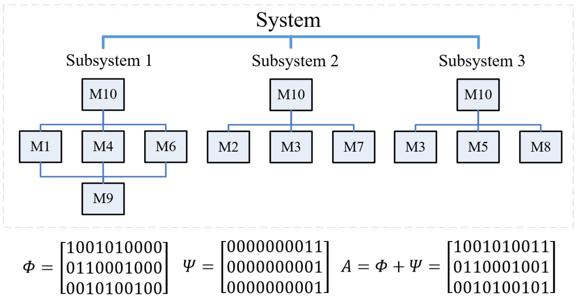
Suppose that a software system is developed based on common modular components. The methodology of modular software development emphasizes splitting software systems into independent, interchangeable modules. The modules contain everything that is essential to execute a single aspect of the functionality of the software. Accordingly, a modular software system allows for being divided by splitting down a whole system into smaller software modules in order to execute a variety of tasks. This enables software staff to work simultaneously and minimizes the time taken for development. Based on the above mentioned, the relation among subsystems and common software modules in series and parallel can be seen in Figure 2. In order to apply the relation of the subsystems in mathematics, a matrix would be needed to express this. Please see the bottom of Figure 2, which presents the matrices ($\Phi$, $\Psi$, and $A$) and illustrates the relationship among subsystems and common modules.

In this situation, the manager of software development has to begin the testing and debugging work for different software modules at the same time in order to shorten the amount of testing time for the whole project. As a result, the individual software module can be assigned to one of the testing groups so that the time frame can be shortened. Figure 3 illustrates the concept of such parallel testing work. Although the manager tries to shorten the project’s testing time for releasing his developed software system as soon as possible, he still has to maintain the software reliability above an acceptable level to avoid user dissatisfaction. Based on the above reasons, the manager needs to consider how to balance the testing time and the system reliability before he makes the best schedule for the testing project. The bottom of Figure 3 illustrates the time frame of the testing project with the individual software module’s reliability and mean value.

Table 2. The Terminologies and Notations.

-Sets

$i$: the indicator of subsystem ($i=1\dots n$) $j$: the indicator of software module ($j=1\dots m$) $p$: the indicator of testing staff group ($p=1\dots q$)

-Decision Variables

$X_{jp}$: $X_{jp}\in \left\{0\mathrm{or}1\right\}$; $X_{jp}=1$ represents that software module $j$ is assigned to the testing group $p$ $T_j$: the testing time of software module $j$ $T{S}_p$: the testing time of the testing group $p$ $R_i$: the software reliability of subsystem $i$

-Parameters & Functions

${\alpha }_p$: the autonomous errors-detected factor of the testing group $p$ ${\beta }_p$: the learning factor of the group of testing group $p$ $a_j$: the expected number of all potential errors in software module $j$ $M\left(T_j,a_j, {\alpha }_p,{\beta }_p\right)$: the mean value function with the parameters $a_j$, ${\alpha }_p$, ${\beta }_p$ and testing time $T_j$ $D\left(T_j\right)$: the function of the error detection rate $R\left(x|T_j,a_j,{\alpha }_p,{\beta }_p\right)$: the software reliability with the parameters $x$, $a_j$, ${\alpha }_p$, ${\beta }_p$ and testing time $R_i^0$: the minimal reliability requirement of subsystem $i$ $\lambda \left(T_j\right)$: the intensity function is used to represent the number of errors that are detected at a specific time ($T_j$) ${\Phi }_{ij}$: ${\Phi }_{ij}\in \left\{0\mathrm{or}1\right\}$; ${\Phi }_{ij}=1$ represents that subsystem $i$ connects software module $j$ in parallel. The form of the parameters can be presented as a matrix as follows: $\Phi =\left[\begin{array}{c}1001010000\\ 0110001000\\ 0010100100\end{array}\right]$ (the mapping structure can be seen in Figure 2) ${\Psi }_{ij}$: ${\Psi }_{ij}\in \left\{0\mathrm{or}1\right\}$; ${\Psi }_{ij}=1$ represents that subsystem $i$ connects software module $j$ in series. The form of the parameters can be presented as a matrix as follows: $\Psi =\left[\begin{array}{c}0000000011\\ 0000000001\\ 0000000001\end{array}\right]$ (the mapping structure can be seen in Figure 2) $A_{ij}$: $A_{ij}\in \left\{0\mathrm{or}1\right\}$; $A_{ij}=1$ represents that subsystem $i$ connects software module $j$ no matter what it is in series or parallel. The form of the parameters can be presented as a matrix as follows: $A=\Phi +\Psi =\left[\begin{array}{c}1001010011\\ 0110001001\\ 0010100101\end{array}\right]$ (the mapping structure can be seen in Figure 2) $T{S}_0$: the requirement of time limit for the tesing project $S{C}_p$: the setup cost by testing group $p$ $G{C}_p$: the routine cost by testing group $p$ $D{C}_p$: the cost to removing a software bug by testing group $p$ $R{C}_i$: the risk cost for the subsystem $i$ $OC\left(T{S}_p\right)$: the function of the opportunity cost after software release, and it is optional for the total testing cost.

presents the terminologies and notations which will be used in the proposed models:

In this section, the objective of this study is to present two mathematical models which are proposed for different purposes. Model 1 is for minimizing the time frame of the software testing project under the requirement of every subsystem reliability $R_i^0$. The mathematical programming model can be given as follows:

Model 1:

$$Min\left\{Max\left\{T{S}_1,T{S}_2,\dots ,T{S}_q\right\}\right\}$$

(28)

Subject to:

$$R_i=\left\{\begin{array}{c}{\displaystyle {\displaystyle \prod }_{p=1}^P}{\displaystyle {\displaystyle \prod }_{j=1}^J}\left\{{\Psi }_{ij}{X}_{jp}R\left(x|T_j,a_j,{\alpha }_p,{\beta }_p\right)+\left(1-{\Psi }_{ij}{X}_{jp}\right)\right\}\\ \times \left\{1-{\displaystyle {\displaystyle \prod }_{p=1}^P}{\displaystyle {\displaystyle \prod }_{j=1}^J}\left\{1-{\Phi }_{ij}{X}_{jp}R\left(x|T_j,a_j,{\alpha }_p,{\beta }_p\right)\right\}\right\}\end{array}\right\},i=1\dots n$$

(29)

$$R_i\ge R_i^0,i=1\dots n$$

(30)

$${\displaystyle \sum }_{p=1}^q{X}_{jp}=1,j=1\dots m$$

(31)

$${\displaystyle \sum }_{j=1}^m{X}_{jp}{T}_j=T{S}_p,p=1\dots q$$

(32)

The objective Function (28) is to minimize the time length of the project under multiple testing staff groups. Constraint (29) is used to calculate the reliability of each subsystem reliability. Constraint (30) is to ensure that the reliability of each subsystem must meet the minimal requirement $R_i^0$. Constraint (31) is to ensure that each module can only be assigned to a specific testing group. Constraint (32) is used to calculate the time length for each testing group.

Model 2 is for minimizing the total testing cost under the minimal requirement of the system reliability $R_i^0$ and the time limit of the testing project $T{S}_0$. The mathematical programming model can be given as follows:

Model 2:

$$MinTC={\displaystyle {\displaystyle \sum }_{j=1}^m}{\displaystyle {\displaystyle \sum }_{p=1}^q}{X}_{jp}\left(S{C}_p+G{C}_p{T}_j+D{C}_{p}M\left(T_j,a_j,{\alpha }_p,{\beta }_p\right)\right)+{\displaystyle {\displaystyle \sum }_{i=1}^n}R{C}_i\left(1-R_i\right)+OC\left(T{S}_p\right)$$

(33)

Subject to:

$$R_i=\left\{\begin{array}{c}{\displaystyle {\displaystyle \prod }_{p=1}^P}{\displaystyle {\displaystyle \prod }_{j=1}^J}\left\{{\Psi }_{ij}{X}_{jp}R\left(x|T_j,a_j,{\alpha }_p,{\beta }_p\right)+\left(1-{\Psi }_{ij}{X}_{jp}\right)\right\}\\ \times \left\{1-{\displaystyle {\displaystyle \prod }_{p=1}^P}{\displaystyle {\displaystyle \prod }_{j=1}^J}\left\{1-{\Phi }_{ij}{X}_{jp}R\left(x|T_j,a_j,{\alpha }_p,{\beta }_p\right)\right\}\right\}\end{array}\right\},i=1\dots n$$

(34)

$$R_i\ge R_i^0,i=1\dots n$$

(35)

$${\displaystyle \sum }_{p=1}^q{X}_{jp}=1,j=1\dots m$$

(36)

$${\displaystyle \sum }_{j=1}^m{X}_{jp}{T}_j=T{S}_p,p=1\dots q$$

(37)

$$T{S}_p\le T{S}_0,p=1\dots q$$

(38)

The objective Function (33) is for minimizing the total testing cost under a modular software system. Constraint (34) is the same as Constraint (29) to calculate the reliability of each subsystem reliability. Constraint (35) is also the same as Constraint (30) to ensure that the reliability of each subsystem meets the minimal requirement. Constraint (36) is the same as Constraint (31) to ensure each module only can be assigned to a specific testing group. Constraint (37) is the same as Constraint (32) is for calculating the total testing time for every group of testing staff. Constraint (38) is to ensure that the testing time length cannot exceed the time limit of the project.

3.3. Computerized Decision Support System Design

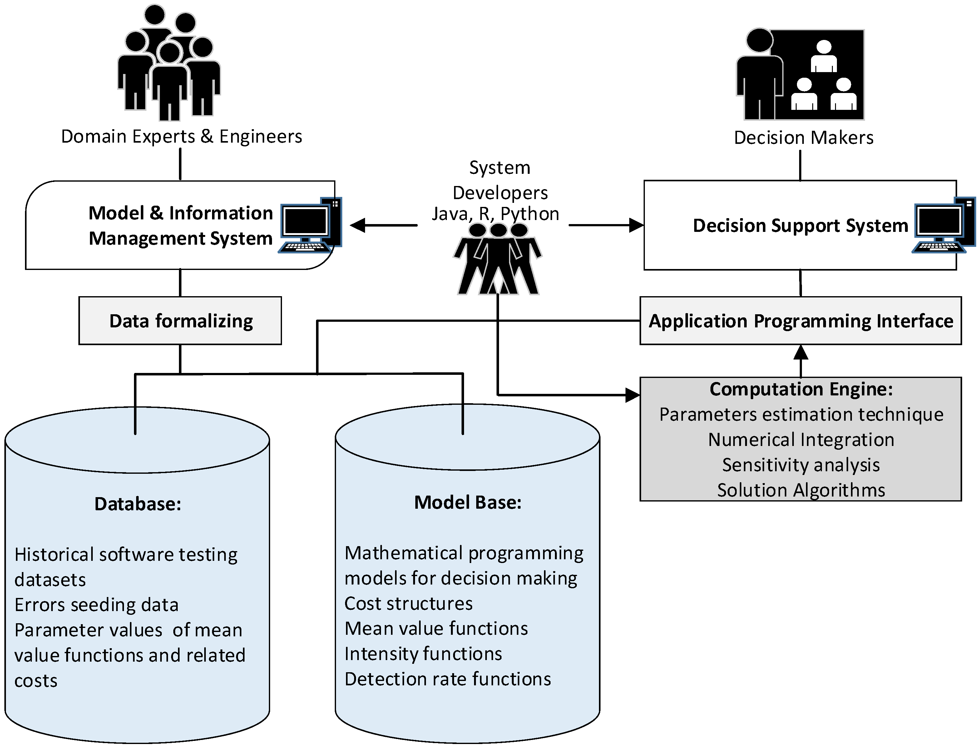
In dealing with these mathematical programming problems, a computerized application system is necessary to implement the problem-solving process to obtain the optimal decision for software release. To improve the efficiency of the system, some components should be included in the designed system. In this study, these components are a designed database, a model base, a data formalizing program module, a specific application programming interface, and a designed computation engine.

The database is designed to store the parameters regarding the related costs and various systems’ historical testing data. Similarly, the model base is designed to store the various mathematical decision models of the software release policies. The data formalizing mechanism would be necessary for us to transform the inconsistent data into a more usable state when storing or accessing the database and model base, and a data formalizing program module would assist us with storing or accessing the data more effectively and efficiently.

Moreover, solving the proposed models requires mathematical programming algorithms and numerical integration; a powerful computation engine is needed to construct the system. The computation engine can be developed by internal programmers or obtained from external software providers (e.g., from Python and R packages). For the purpose of utilizing a computation engine more efficiently and conveniently, the mechanism of an application programming interface is a best way of exchanging information between the designed system and a computation engine, and in the following section we introduce the system design, and detail implementation.

There are two subsystems within the whole system which have been organized in order to enhance its manageability. In order to maintain the database and model base, the model management system was designed to be used by software engineers, domain experts, and testing staff. This decision support system is designed to provide decision makers useful information for related testing schedules and work.

In operating the model management system, the engineers first gather historical data from former software testing projects, and also choose possible SRGMs and inspect the cost structure. The engineers can then store the related data in the database through the model management system. Moreover, due to the fact that the efficiency of software testing work to the testing staff is extremely important to the estimated software test cost, the domain experts would determine which SRGM would fit to estimate the case of each software testing project. It is important to note that due to commercial confidentiality, the engineers, domain experts, and technical managers should only have access to their own subsystems as a matter of precaution. In regards to the mathematical programming models (excluding the parameters), these are usually established by the system programmers right after the system has been developed and are part of the model base.

The decision support system is designed to assist managers in making decisions in the upper management, and it provides complete and integrated information that can be used to make informed decisions. It provides decision makers with the opportunity to analyze all the constructive information contained in the database as well as the model base, and to use this information to determine accurately and confidently the best decision to take. Since some decision support systems have been successfully applied in the field of Industry 4.0, the experience and the conceptual design of decision support systems with Industry 4.0 can be a reference for the system development [43,44,45,46,47,48]. In order to achieve an optimal decision, however, it may be necessary to use a computation engine that can handle the complexity inherent in obtaining such a decision. With the use of an application programming interface (API), we are able to access different computation program objects that have been developed by external or internal developers quite easily. In Figure 4, it can be seen that a schematic representation of our system’s implementation architecture.

4. Application and Numerical Analysis

Suppose that a technology company was developing an Engineering Data Analysis System (EDA). After fourteen months of software development, it is ready for the final software testing and debugging phase. Most clients and users want the software to be at least 95% reliable during the operation time, which means that there should be no more than 5% chance of software errors during the one-hour operation time. Accordingly, the managers of the technology company must propose a software testing project to improve the reliability and quality of the EDA system.

Furthermore, based on the historical testing datasets of the company’s testing teams, it can be understood that different testing teams or different scales of manpower will affect the efficiency of software debugging. Accordingly, the managers of the technology company propose a testing project in considering their manpower to achieve the objectives of lower cost and higher reliability. After investigation and evaluation by the company’s senior engineers and domain experts, the information and estimated parameters for the software testing project can be seen in

Table 3. Related parameters setting for the testing project of the EDA system.

Parameter	Value
$a$ (the number of potential errors in the sytem)	4130
${\alpha }_p$ (the autonomous errors-detected factor)	0.25
${\beta }_p$ (the learning factor)	0.13
$S{C}_p$ (the setup cost)	$18,750
$G{C}_p$ (the routine cost with testing time)	$2500/per day
$D{C}_p$ (the cost of removing software bugs)	$56
$RC$ (the risk cost)	$720,000 ($7200 reputation loss vs. 1% reliability)
$x$ (the defined operation time without any error)	1 h
$R^0$ (the minimal requirement of the sytem reliability)	0.95

.

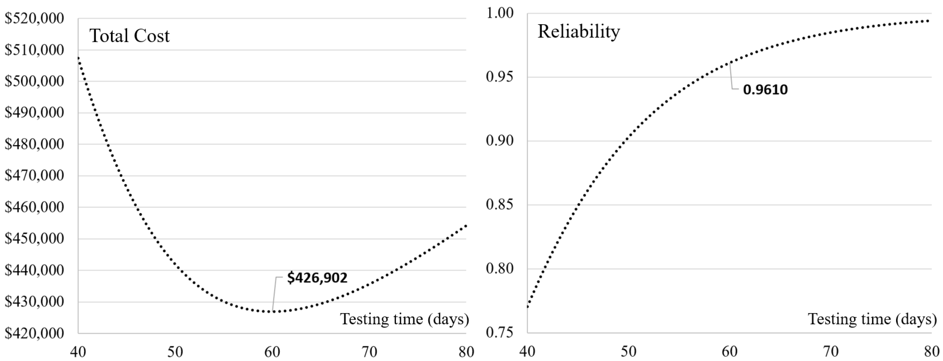
Following the completion of the calculation utilizing the proposed model, the curve of the expected testing cost of the project presents convexity with testing time, as can be seen in Figure 5 and

Table 4. Computation results of the total testing cost, the mean value, and the error detection rate.

$\mathit{T}$	$\mathit{T}\mathit{C}\left(\mathit{T}\right)$	$\mathit{R}\left(\mathit{x}|\mathit{T},\mathit{a},{\mathit{\alpha }}_{\mathit{p}},{\mathit{\beta }}_{\mathit{p}}\right)$	$\mathit{D}\left(\mathit{T}\right)$	$\mathit{T}$	$\mathit{T}\mathit{C}\left(\mathit{T}\right)$	$\mathit{R}\left(\mathit{x}|\mathit{T},\mathit{a},{\mathit{\alpha }}_{\mathit{p}},{\mathit{\beta }}_{\mathit{p}}\right)$	$\mathit{D}\left(\mathit{T}\right)$
41	$497,590	0.7887	0.094006	61	$427,020	0.9645	0.09485
42	$488,614	0.8055	0.094095	62	$427,345	0.9677	0.094864
43	$480,415	0.8212	0.094176	63	$427,860	0.9705	0.094876
44	$472,960	0.8357	0.09425	64	$428,548	0.9732	0.094887
45	$466,218	0.8492	0.094318	65	$429,395	0.9756	0.094897
46	$460,152	0.8617	0.094379	66	$430,387	0.9777	0.094907
47	$454,728	0.8733	0.094435	67	$431,513	0.9797	0.094915
48	$449,908	0.8840	0.094486	68	$432,760	0.9816	0.094923
49	$445,655	0.8938	0.094532	69	$434,118	0.9832	0.09493
50	$441,934	0.9029	0.094575	70	$435,578	0.9847	0.094936
51	$438,709	0.9112	0.094613	71	$437,130	0.9861	0.094942
52	$435,947	0.9189	0.094648	72	$438,767	0.9873	0.094947
53	$433,615	0.9259	0.09468	73	$440,481	0.9885	0.094952
54	$431,681	0.9323	0.094709	74	$442,265	0.9895	0.094956
55	$430,115	0.9382	0.094735	75	$444,113	0.9905	0.09496
56	$428,891	0.9436	0.094759	76	$446,019	0.9913	0.094964
57	$427,982	0.9486	0.094781	77	$447,979	0.9921	0.094967
58	$427,362	0.9531	0.094801	78	$449,988	0.9928	0.09497
59	$427,010	0.9573	0.094819	79	$452,040	0.9935	0.094973
60	$426,902	0.9610	0.094835	80	$454,133	0.9941	0.094975

. In order to meet the minimal requirement of software reliability ($R^0\ge 0.95$), the testing time should be set to 58 days or later ($R\left(x|T,a,{\alpha }_p,{\beta }_p\right)=0.9531$). However, the time point ($T=58$) is not the optimal solution for the company since the expected testing cost (USD 427,362) of the time point is still higher than that of the next day (USD 427,010). Therefore, the managers should set the testing time to 60 days after the testing project begins, and the expected testing cost will decline to USD 426,902 with the software reliability 0.9610. The benefit of extending the testing time for increasing reliability can cover the loss of other growing costs. Additionally, it can be seen that the detection rate $D\left(T\right)$ is relatively stable with testing time because the value of the learning factor is very low and most testing staff cannot effectively increase debugging efficiency from their experience in the past.

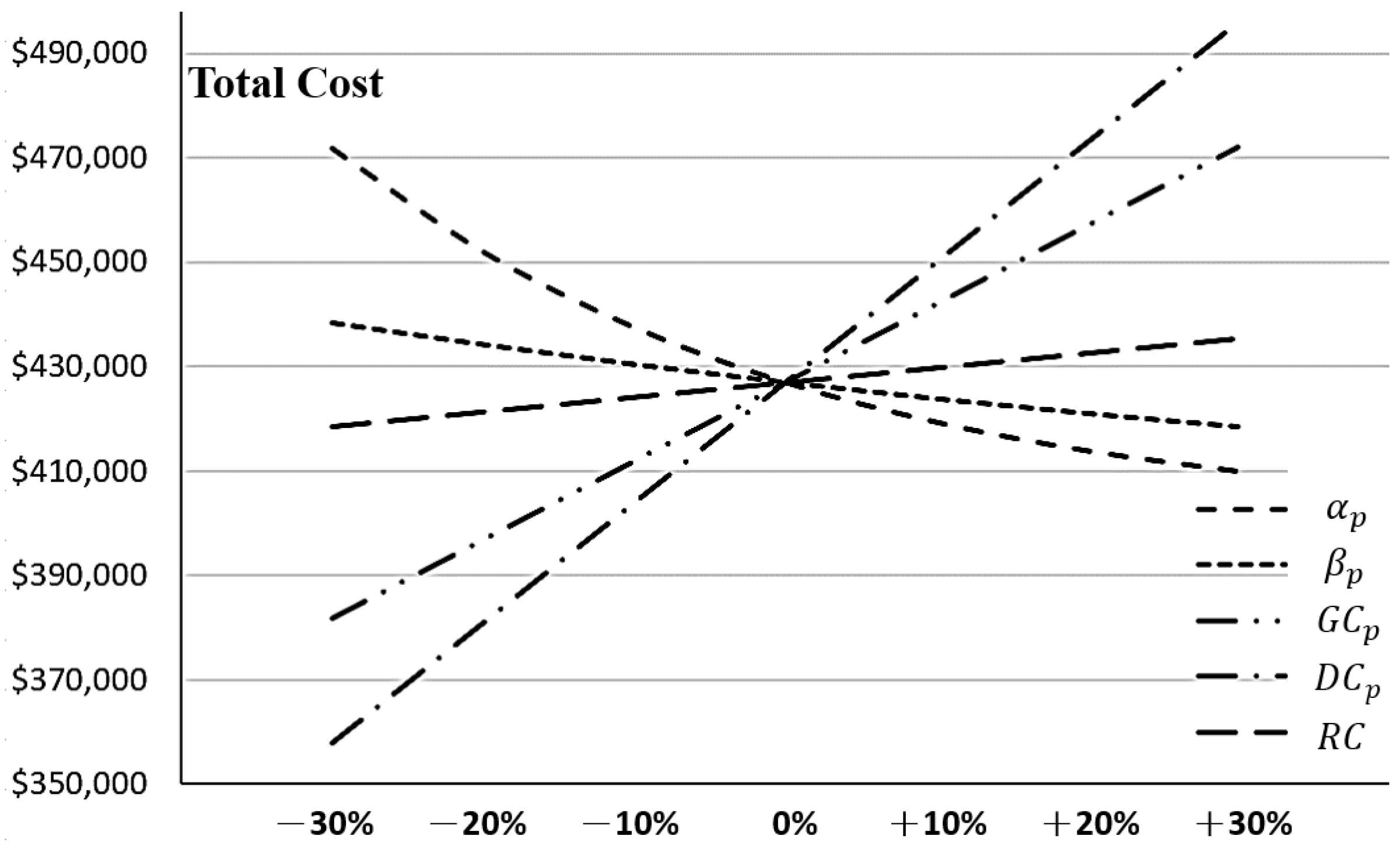
There were a few crucial parameters that were taken into consideration, and a sensitivity analysis was carried out in order to explore the influence of these parameters on the total cost under the optimal software release time. Figure 6 presents the sensitive analysis results for the related parameters ${\alpha }_p$, ${\beta }_p$, $G{C}_p$, $D{C}_p$, and $RC$. As can be seen in Figure 6, in the comparison of the parameters of the mean value function, ${\alpha }_p$ is more sensitive to ${\beta }_p$ because the value of parameter ${\beta }_p$ is relatively low and cannot get a multiplicative effect with ${\alpha }_p$. Therefore, if the condition ${\beta }_p>{\alpha }_p$ can be satisfied, the learning effect is significant enough to accelerate the efficiency of debugging work. Moreover, misestimating ${\alpha }_p$ and ${\beta }_p$ will disturb the testing project’s budget plan. In order words, if the manager overestimates ${\alpha }_p$ and ${\beta }_p$, it will cause an underestimation of the testing cost. Furthermore, the misestimating of ${\alpha }_p$ and ${\beta }_p$ would also impact on the release decision. For an example, if the manager overestimates ${\alpha }_p$ and ${\beta }_p$, he/she will shorten the planned testing time and rush to release the software system. Such an outcome may cause clients’ dissatisfaction and damage the company’s reputation due to the unreliable system released. How can the manager increase the testing efficiency? The manager can provide more job training to the testing staff in advance, but it also increases the expenditure in job education. Even if the investment in job education can effectively increase ${\alpha }_p$ and ${\beta }_p$, the manager still considers the trade-off between the investment in the staff’s skills and the benefit from reliability improvement and cost reduction. Additionally, the time-dependent routine cost $G{C}_p$ and the debugging cost $D{C}_p$ will also influence the testing cost. In this case, reducing 30% of the routine cost can save about 10.5% of the testing cost. However, saving the debugging cost can have a better effect on reducing the testing cost since a 30% deduction of the debugging cost can save 16% of the testing cost. Accordingly, the manager must take all the factors into consideration to make an appropriate decision for the testing work.

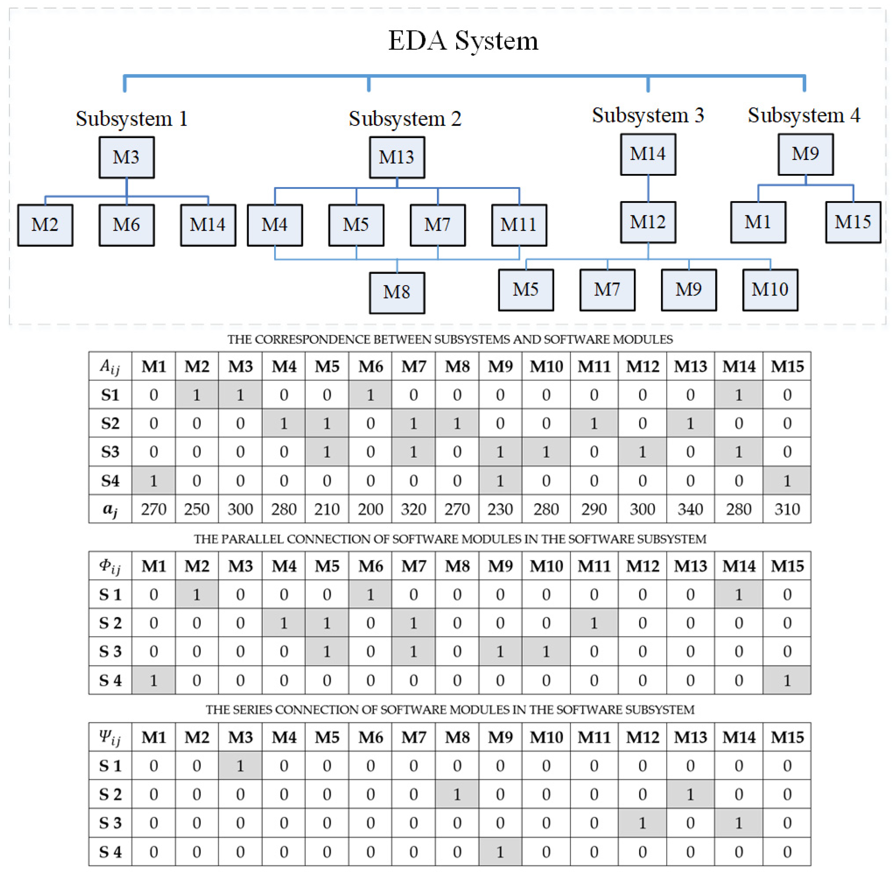
Furthermore, suppose the technology company decided to develop software systems using modular programming instead of traditional system development. Therefore, the whole EDA system can be divided into the four subsystems and the fifteen related software modules. Figure 7 illustrates that each subsystem can utilize some software modules in series-parallel relations. The correspondence between the subsystem and the software modules can be tabulated as a matrix. The bottom half of Figure 7 gives the matrices of $\Phi$, $\Psi$, and $A$ for illustrating the structures of subsystems and modules. The initial potential software errors of each subsystem have been estimated by senior engineers and are presented at the bottom of matrix $A$. Moreover, in this figure, it can be seen that the common and shared modules M5, M7, M9, and M14 can be used in different subsystems. Therefore, such a common and shared module’s reliability will influence more than one subsystem’s reliability. Similar to the previous issue, the software testing phase will begin after fourteen months of software development. Instead, the manager adopts the modular testing strategy for the EDA system in parallel. At present, according to the company’s human resources, three software testing and debugging groups can be assigned to the testing and debugging work for 8 h per day. The model parameters (${\alpha }_p$ and ${\beta }_p$) of each testing and debugging group can be estimated according to the historical testing data. Furthermore, due to the different testing and debugging efficiency for each group, the related costs must be different. The above information can be seen in

Table 5. The parameter values regarding each testing staff groups’ efficiency and costs.

Parameters	Testing Staff 1	Testing Staff 2	Testing Staff 3
${\alpha }_p$	0.28	0.31	0.35
${\beta }_p$	0.18	0.20	0.23
$S{C}_p$	950	1200	1600
$G{C}_p$	580	620	640
$D{C}_p$	42	45	48

. Moreover, each subsystem has its minimal reliability requirement, and the manager must fulfill the basic requirement of clients. The risk costs of each subsystem are estimated to be USD 140,000, USD 180,000, USD 190,000, and USD 210,000, individually. It should be noted that the reliability calculation is based on no error occurring within a defined operation time. Finally, the manager is required to shorten the length of the testing project, and therefore the upper limit of the testing time frame is set to 45 days. The detailed information can be seen in

Table 6. The information of the minimal requirement of reliability, the risk cost, and the upper limit of testing time frame.

	Subsystem 1	Subsystem 2	Subsystem 3	Subsystem 4
Minimal requirement of subsystem reliability$i$: $R_i^0$	0.95	0.90	0.90	0.90
The risk cost of subsystem $i$: $R{C}_i$	$140,000	$180,000	$190,000	$210,000
upper limit of testing time frame $T{S}_0=45 days$; Operation time with no error $x=1$ h

.

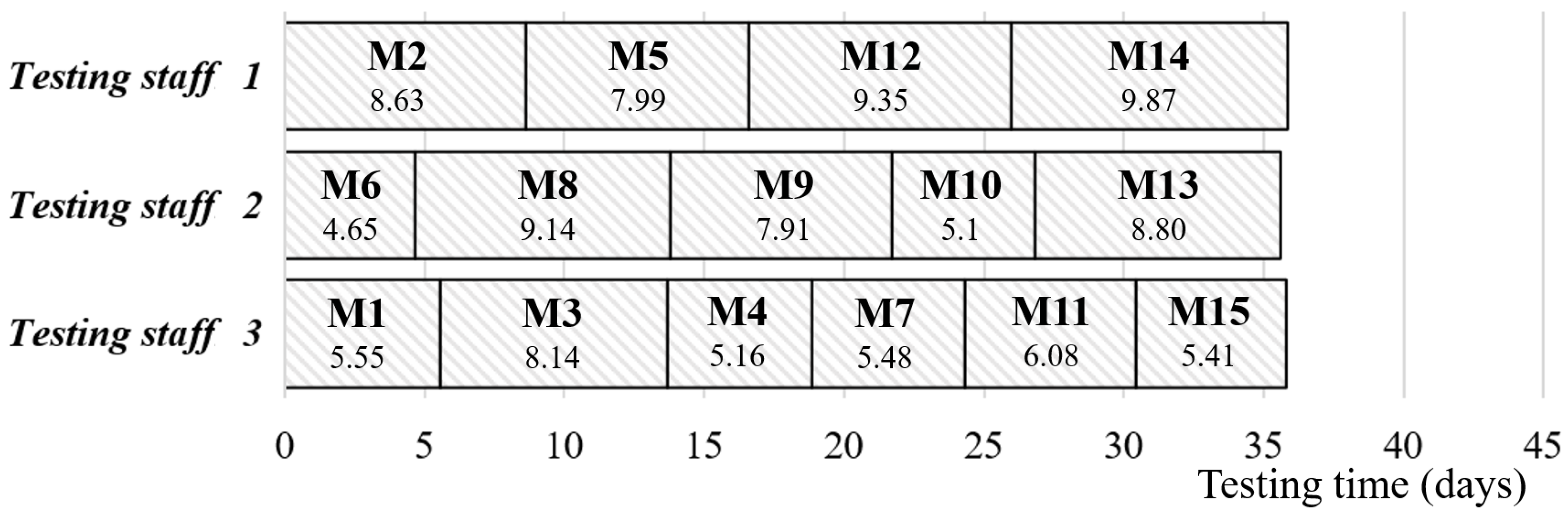
Suppose the manager of the company would like to know how to schedule the testing work in order to get the shortest time frame for the EDA system testing. Therefore, the manager can apply Model 1 of Section 3.2 in dealing with the problem. After the calculation using Model 1, we can get the optimal solution of the software test scheduling. Figure 8 and

Table 7. The computation results of the software test scheduling by applying Model 1.

Module	M1	M2	M3	M4	M5	M6	M7	M8	M9	M10	M11	M12	M13	M14	M15
Assign to Group p	3	1	3	3	1	2	3	2	2	2	3	1	2	1	3
Testing Time/Days	5.55	8.63	8.14	5.16	7.99	4.65	5.48	9.14	7.91	5.1	6.08	9.35	8.80	9.87	5.41
Reliability of Module j	0.8219	0.9329	0.9507	0.7779	0.9252	0.7578	0.7852	0.9588	0.9358	0.7508	0.8551	0.9415	0.9391	0.9566	0.7849
Average Reliability: 0.9125; Reliability of subsystem i: $R_1^s$ = 0.95, $R_2^s$ = 0.90, $R_3^s$ = 0.90, $R_{4 }^s$ = 0.90 Total cost = $328,935 Time frame for staff groups p: $T{S}_1$ = 35.83 days (for modules: 2, 5, 12, 14), $T{S}_2$ = 35.82 days (for modules: 6, 8, 9, 10, 13), $T{S}_3$ = 35.83 days (for modules: 1, 3, 4, 7, 11, 15)

present the Gantt chart and the detailed computation results of the software test scheduling by applying Model 1. In this figure, we can see that the manager should assign modules M2, M5, M12, and M14 to staff group 1, modules M6, M8, M9, M10, and M13 to staff group 2, and modules M1, M3, M4, M7, M11, and M15 to staff group 3. The testing time can be shortened to 35.83 days. However, the averaged reliability of the whole system will be down to 0.9125 (Reliability of subsystem: $R_1^s$ = 0.95, $R_2^s$ = 0.90, $R_3^s$ = 0.90, $R_{4 }^s$ = 0.90), and the total cost will be estimated at USD 328,935. Although Model 1 can effectively shorten the testing time of the project, the averaged system reliability is relatively low, and the testing cost needs to reach the optimum. Accordingly, Model 1 is only appropriate for a software development project that needs to be released as soon as possible.

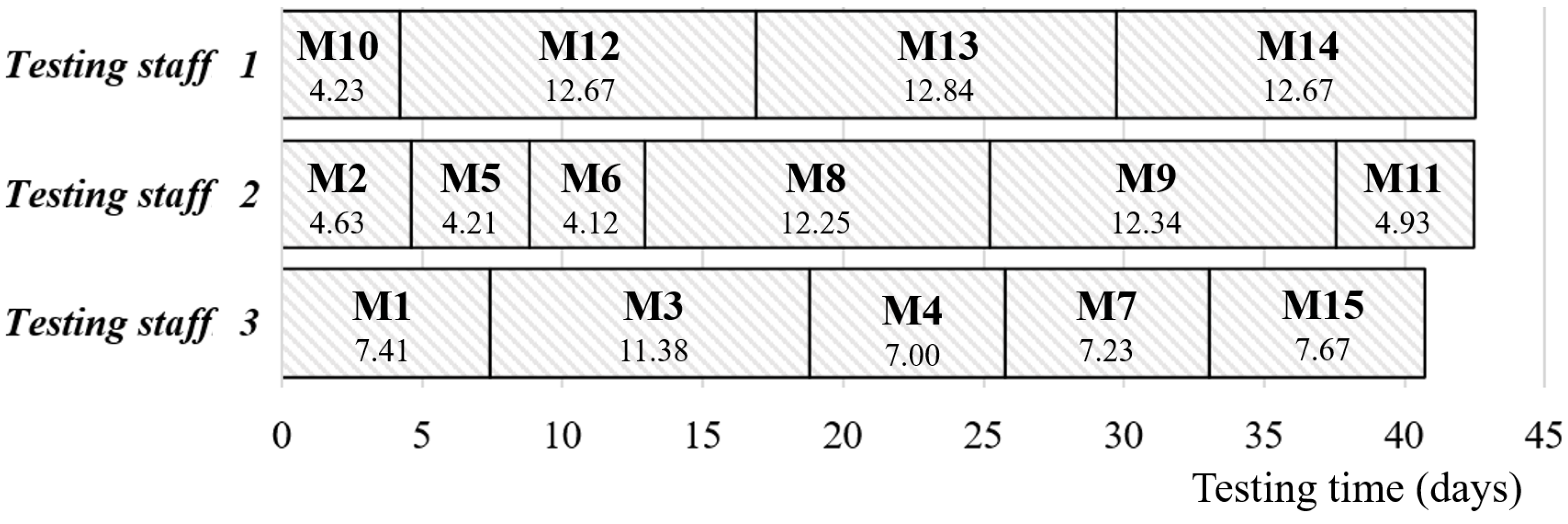
Suppose the manager changes his/her mind to adopt the strategy of minimizing the testing cost. Therefore, Model 2 of Section 3.2 can be applied to optimize the testing work. After the calculation of Model 2, the optimal solution regarding the staff schedule, total cost, the time frame for each testing staff group, and each subsystem’s reliability can be seen in Figure 9 and

Table 8. The computation results of the software test scheduling by applying Model 2.

Module	M1	M2	M3	M4	M5	M6	M7	M8	M9	M10	M11	M12	M13	M14	M15
Assign to Group p	3	2	3	3	2	2	3	2	2	1	2	1	1	1	3
Testing Time/Days	7.41	4.63	11.38	7.00	4.21	4.12	7.23	12.25	12.34	4.23	4.93	12.67	12.84	12.76	7.67
Reliability of Module j	0.9334	0.7054	0.9922	0.9137	0.7016	0.7047	0.9137	0.9913	0.9929	0.6034	0.7023	0.9868	0.9862	0.9882	0.9340
Average Reliability: 0.9830; Reliability of subsystem i: $R_1^s$ = 0.9912, $R_2^s$ = 0.9770, $R_3^s$ = 0.9752, $R_4^s$ = 0.9886 Total cost = $284.418 Time frame for staff groups p: $T{S}_1$ = 42.5 days (for modules: 10, 12, 13, 14), $T{S}_2$ = 42.5 days (for modules: 2, 5, 6, 8, 9, 11), $T{S}_3$ = 40.7 days (for modules: 1, 3, 4, 7, 15)

. In Figure 7, the manager should assign modules M10, M12, M13, and M14 to staff group 1, modules M2, M5, M6, M8, M9, and M11 to staff group 2, and modules M1, M3, M4, M7, and M15 to staff group 3. The testing time of the project will be extended to 42.5 days. Even though the testing time will be longer, the averaged reliability of the whole system will be improved to 0.9830 (Reliability of subsystem: $R_1^s$ = 0.9912, $R_2^{s }$ = 0.9770, $R_3^{s }$ = 0.9752, $R_4^s$ = 0.9886), and the total cost will be decreased to USD 284.418. From the perspective of cost and software quality, the strategy of Model 2 seems beneficial to the company; however, the manager needs to delay the release of the EDA system by about 18.62%. However, if the deadline issue is really important and the manager must fulfill the contract to avoid the loss of the company’s goodwill, the manager may take a tradeoff strategy between Model 1 and Model 2′s objectives. Accordingly, the manager should adjust his/her original decision to adapt to different situations in practice. Based on the above mentioned, the proposed models can effectively improve the quality and schedule of the software testing work to enhance the software system’s competitiveness.

5. Conclusions

Software reliability and quality are critical for evaluating the success of software development. Software testing work is a meaningful way to improve stability for ensuring the quality of software. However, due to the pressure of the software release schedule and the constraint of the testing project budget, the manager must develop effective strategies to make appropriate trade-offs between software quality and testing cost. In the past, the majority of research on software system testing was centered on determining the best testing schedule for a single software system. Consequently, there was significantly less discussion on how to arrange the testing schedule under modular software system development. In this scenario, the manager must understand how to allocate and arrange the necessary testing resources among all software subsystems and modules. As a result, in this work, two programming models with consideration of learning effect have been proposed to deal with the scheduling issue of modular software system testing in order to achieve the shortest testing time with limited testing resources and meet specified reliability requirements.

According to the analysis results of the study, the managerial implications and suggestions can be summarized as follows: (1) In order to increase the value of the model’s parameters ${\alpha }_p$ and ${\beta }_p$, it will be necessary to hire more senior testing staff or provide on-the-job training to those already working on the project. This, in turn, needs an increased budget for the project to cover these costs. As a result, the software developer has to take into consideration the trade-offs in order to come up with a balanced decision. (2) Software release timing is not only a matter of cost, as the software provider must also meet the minimum level of software reliability in accordance with the contract or most customers’ requirements. (3) In general, the detection rate is relatively stable with testing time. If the manager wants to raise the detection rate in the later phase, the learning factor ${\beta }_p$ needs to be higher than the autonomous errors-detected factor ${\alpha }_p$ since it will not get a multiplicative effect with ${\alpha }_p$ as long as ${\beta }_p$ is relatively low. (4) Model 1 can effectively shorten the testing period but it may sacrifice the software reliability and quality because the model only fulfills the minimal requirement of software reliability. Accordingly, Model 1 is only appropriate for a project that needs to be released as soon as possible. Otherwise, the manager needs to relax the constraint of each subsystem’s reliability requirement. (5) Model 2 focuses on minimizing the total testing cost. However, if the deadline is really important and the manager needs to fulfill the contract to maintain the company’s reputation, the manager may choose a strategy that compromises between Model 1 and Model 2’s objectives. With the above considerations, the proposed models can be utilized effectively to enhance the company’s competitiveness by improving the quality of software testing work.

Finally, some directions can be considered for future studies: (1) It is possible to integrate an NHPP with covariates into a software reliability growth model. With the help of the NHPP with covariates, the extra failure data (testing effort, testing resources, etc.) can be used to adjust the original prediction, and thus the accuracy of the prediction will be increased by the model. (2) Due to the fact that the execution time of the two mathematical programming models would be increasing exponentially with the problem size, developing efficient solutions would be necessary. Genetic algorithms, particle swan optimization, other heuristic algorithms, etc., may be a direction for improving the efficiency of the model’s calculation. (3) In the development of a software reliability growth model, the issue of a debugging time delay can be considered. The majority of studies conducted in the past assumed the error correction time would not have any impact on the testing process in the future. However, such an assumption is unrealistic. In the future, we will revise the unrealistic assumptions in order to develop a new model that is more realistic.