Symmetries of Quantum Fisher Information as Parameter Estimator for Pauli Channels under Indefinite Causal Order

Abstract

Quantum Fisher Information is considered in Quantum Information literature as the main resource to determine a bound in the parametric characterization problem of a quantum channel by means of probe states. The parameters characterizing a quantum channel can be estimated until a limited precision settled by the Cramér–Rao bound established in estimation theory and statistics. The involved Quantum Fisher Information of the emerging quantum state provides such a bound. Quantum states with dimension $d=2$, the qubits, still comprise the main resources considered in Quantum Information and Quantum Processing theories. For them, Pauli channels are an important family of parametric quantum channels providing the most faithful deformation effects of imperfect quantum communication channels. Recently, Pauli channels have been characterized when they are arranged in an Indefinite Causal Order. Thus, their fidelity has been compared with single or sequential arrangements of identical channels to analyse their induced transparency under a joint behaviour. The most recent characterization has exhibited important features for quantum communication related with their parametric nature. In this work, a parallel analysis has been conducted to extended such a characterization, this time in terms of their emerging Quantum Fisher Information to pursue the advantages of each kind of arrangement for the parameter estimation problem. The objective is to reach the arrangement stating the best estimation bound for each type of Pauli channel. A complete map for such an effectivity is provided for each Pauli channel under the most affordable setups considering sequential and Indefinite Causal Order arrangements, as well as discussing their advantages and disadvantages.

1. Introduction

Classically, Fisher information is a mathematical statistics indicator to measure the amount of information provided by an observed random variable related with an unknown parameter of a statistical distribution modelling it [1]. Its extension in Quantum Information, the Quantum Fisher information (QFI), enables the estimation of a parameter associated with a quantum process through the measurement of an involved observable [2]. Such a process could represent a quantum operation or a quantum channel characterized by the parameter or parameters to be estimated. Thus, QFI has certain information about the nature of the quantum channel being transited by a given quantum state, thus creating a bound for the knowledge of the channel parameters.

A kind of valuable channel is the family of Pauli channels, the channels involved with the most basic, but more valued construction in quantum information and communication: Qubits. They appear as Local Operations with Classical Communication (LOCC) applied on them. In general, those channels exhibit a multi-parametric characterization based on four parameters (currently only three are independent). In particular, Pauli channels communication properties have been widely analysed due to their affordability [3]. Thus, for quantum channel identification problems, the best estimation of such parameters arises naturally to get their best faithful characterization.

Despite direct characterization of such channels being an interesting problem, another alternative approach considers arrangements for identical channels, such as the use of sequential redundant channels or otherwise Indefinite Causal Order arrangements (ICO). Whichever naturally includes the single arrangement case, such arrangements are introduced to hopefully improve the parameter estimation of the single channels conforming them. Particularly, ICO arrangements have been introduced in recent years, attributing notable properties to them of improving communication [4,5,6] and being proposed as experimental methods [7]. Then, it is naturally expected that they exhibit certain notable properties to improve the quantum parameter estimation of their components. To afford their theoretical analysis, different treatments have been developed [8,9,10].

In the latest trend, most recently, Pauli channels have been studied under sequential and ICO arrangements to parametrically characterize their communication performance. For ICO, such an analysis enabled the finding of interesting and notable properties, such as induced transparency as a function of the set of parameters characterizing them [11]. Such arrangements can be now analysed in terms of the QFI to compare the affordability of such a family of channels to be characterized by using specific quantum probe states. One of the main objectives in the current analysis is to determine if ICO also improves the outcomes in such a quantum estimation parameter task as compared with the single use of channels or with sequential arrangements, as was comparatively studied in [11]. For such a task, sequential arrangements could also provide notable outcomes due to the repeated output feedback.

The aim of this article is to extend the analysis performed in [11] by studying the properties of Pauli channels under sequential and ICO arrangements of identical Pauli channels, but in this case centered on the Quantum Parameter Estimation (QPE) problem. It is reached by means of the fingerprints settled on specific probe states transiting them. Section 2 presents brief introductions to (a) QFI, (b) its relationship with QPE, (c) basic theory of Pauli channels, and (d) QFI for such specific systems involved: mixed qubit states. Section 3 presents the main treatment for those two types of composed arrangements considering Pauli channels: (a) the sequential arrangement and the ICO arrangement. In both cases, we develop expressions useful for the calculation of QFI. Particularly, we extend the analysis that was begun in [11] with novel outcomes for ICO involving Pauli channels, useful for the characterization of such arrangements. Section 4 includes expressions to obtain QFI in both cases being analysed, together with an insight based on QPE with a single parameter. Then, Section 5 includes the analysis of QFI on the entire parameter space (it means multi-parametric) characterizing Pauli channels in terms of QPE for both sequential and ICO arrangements in comparison. Section 6 includes the conclusions for the present report.

2. QFI as Channel Parameter Estimator and Pauli Channels

Fisher information is a measurement of the amount of information provided by a random variable X about a parameter $\theta$ involved in the probabilistic distribution modelling [12]. For instance, in a binomial distribution, the number of successes X in a Bernoulli experiment with a single experiment success probability $\theta$. A sequence of X values carry out information about $\theta$. Then, in principle, it is possible to infer $\theta$ with certain extent from the observation of a statistical series of outcomes for X. Fisher information represents how much information could be provided about the knowledge of $\theta$ through those observables. Thus, it is possible set a bound, the Cramér–Rao bound (CRB) [13], for the variance of any unbiased estimator of $\theta$, which is stated by the inverse of the Fisher information.

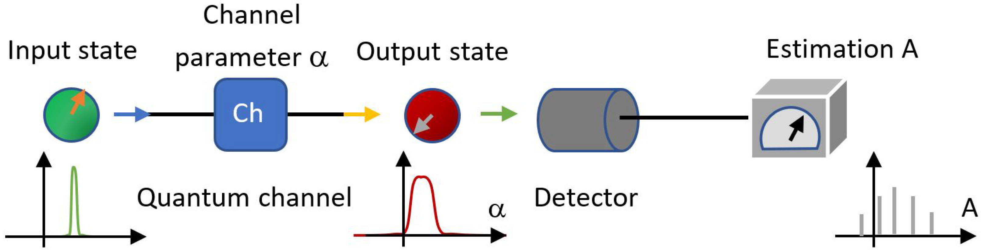
In the current section, we introduce some outcomes involving the quantum version of the Fisher information applied to the transmission of a quantum state through a quantum channel, which could be understood as a stochastic process on an input state ${\rho }_{in}$ generated by the parameters characterizing the channel, while the effects are observed on the output state ${\rho }_{out}$. Figure 1 shows the process. An initial well characterized quantum probe state is sent through a quantum channel being depicted by means of a single parameter $\theta$ or otherwise, by a set of them $\left\{{\alpha }_i\right\}$. The output state, now emerging from it, contains information from those parameters. Thus, it is expected that by selecting certain observable A defined on it, its measurement enables the obtaining of certain light or to infer features of the channel’s nature. Note that both parameters and observables could be independently continuous or discrete.

Together with the last presentation, we will set the main aspects about Pauli channels, together with the main features to get the QFI emerging from those systems and their alternative composed arrangements.

2.1. Quantum Fisher Information

In the multi-parametric version, QFI could be introduced almost as its classical version in terms of the logarithmic derivative [14]. By considering a quantum mixed state $\rho$ emerging from a quantum channel characterized by the set of parameters $({\alpha }_1,{\alpha }_2,{\alpha }_3)$, the entries of the Fisher information matrix is defined by:

$$\begin{array}{c}\hfill {\mathcal{F}}_{ij}\left(\rho \right)=\frac{1}{2}\mathrm{Tr}\left(\rho \{L_i,L_j\}\right)\end{array}$$

(1)

where $L_i$ denotes the logarithmic derivative operator respect to the parameter ${\alpha }_i$, fulfilling:

$$\begin{array}{ccc}\hfill {\partial }_i\rho & =& \frac{1}{2}(\rho L_i+L_i\rho )\hfill \end{array}$$

(2)

thus, other affordable expressions for the Fisher information matrix can be obtained through those definitions:

$$\begin{array}{ccc}\hfill {\mathcal{F}}_{ij}\left(\rho \right)& =& \mathrm{Tr}\left(L_j{\partial }_i\rho \right)\hfill \end{array}$$

(3)

$$\begin{array}{ccc}\hfill {\mathcal{F}}_{ii}\left(\rho \right)& =& \mathrm{Tr}\left(\rho L_i^2\right)\hfill \end{array}$$

(4)

Then, by solving (2) for each $L_i$, we can use (3) to get ${\mathcal{F}}_{ij}\left(\rho \right),i,j=1,2,3$. Despite this, it is easily possible to solve the last equations to find $L_j$ and then to find ${\mathcal{F}}_{ij}\left(\rho \right)$, it could require some algebraic work as a function of the complexity of $\rho$. In fact, depending from the kind of channel being analysed, simpler expressions have been developed to easier the QFI calculation [15]. Below, we develop closer expressions for QFI for the problem being considered in this work.

2.2. Cramér–Rao Bound

The CRB in statistical estimation theory, states a lower bound for the variance of any possible unbiased estimator of a fix deterministic parameter coming from its statistical distribution. Thus, such a variance is at least as high as the inverse of the associated Fisher information [13,16]. Such bound reads for a single parameter distribution:

$$\begin{array}{c}\hfill \mathrm{var}\left(\theta \right)\ge \frac{1}{N\mathcal{F}}\end{array}$$

(5)

where N is the number of repetitions of the estimation experiment (thus, the variance corresponds to that of the mean of estimations for the sample). It only reflects the well-known fact in statistics that the variance for some random variable of a sample is N times that of the population source (under normality). Such an outcome directly extends to QFI, inclusively for a multi-parametric distribution [14], using the QFI matrix $\mathcal{F}\left(\rho \right)$:

$$\begin{array}{c}\hfill \sum _{i_1}^n\mathrm{var}\left({\alpha }_i\right)\ge \frac{1}{N}\mathrm{Tr}\left({\mathcal{F}}^{-1}\left(\rho \right)\right)\ge \frac{1}{N}\sum _{i=1}^n\frac{1}{{\mathcal{F}}_{ii}\left(\rho \right)}\end{array}$$

(6)

In the following, without loss of generality, we will refer just to a single experiment determination or per probe, then $N=1$. As reference, we will call as the hard bound to ${\mathcal{V}}_{\mathrm{h}}\equiv \mathrm{Tr}\left(\left\{{\mathcal{F}}^{-1}\left(\rho \right)\right\}\right)$, while ${\mathcal{V}}_{\mathrm{s}}\equiv {\sum }_{i=1}^n{\mathcal{F}}_{ii}^{-1}\left(\rho \right)$ will be called the soft bound. This last is clearly easier to obtain but imposes a more extreme non-strict bound. The figure of interest in the current work is ${\mathcal{V}}_{\mathrm{h}}$. Note that for a single parameter, both bounds meet ${\mathcal{V}}_{\mathrm{s}}={\mathcal{V}}_{\mathrm{h}}\equiv \mathcal{V}$.

2.3. Pauli Channels in Brief

The general form for a Completely Positive Trace-Preserving (CPTP) map for qubits is given through the Kraus representation [17]:

$$\begin{array}{c}\hfill \Lambda \left[\rho \right]=\sum _{i=0}^3{K}_i\rho K_i^{†}=\sum _{i=0}^3\mathrm{Tr}\left(K_i\rho K_i^{†}\right)\frac{K_i\rho K_i^{†}}{\mathrm{Tr}\left(K_i\rho K_i^{†}\right)}\equiv \sum _{i=0}^3{\mathcal{P}}_i{\rho }_i\end{array}$$

(7)

where $\left\{K_i\right\}$ are the correspondent Kraus operators, a set of four operators $K_i,i=0,1,2,3$ fulfilling the property: ${\sum }_{i=0}^3{K}_i^{†}{K}_i=\mathbf{1}$ (${\sigma }_0$ for qubits), thus preserving the unitary trace of $\Lambda \left[\rho \right]$. Such expression in (7) should be understood as the mixture of four possible states on $\rho$. Then, ${\mathcal{P}}_i=\mathrm{Tr}\left(K_i\rho K_i^{†}\right)$ is the probability related with each one ${\rho }_i$.

The Kraus operators structure depends on the relation between the channel and the environment, together with the basis used to express $\rho$. If the channel just involves LOCC, it could be expressed in terms of unitary operators $U_i$ fulfilling $K_i=\sqrt{{\alpha }_i}{U}_i$ with ${\sum }_{i=0}^3{\alpha }_i=1$.

In the current development, $\rho$ could be expressed in alternative ways depending on the basis used via a unitary basis transformation T as $\rho =T\tilde{\rho }{T}^{†}$. It could be selected transforming the Kraus operators or the unitaries $U_i$. For a LOCC on qubits, the $SU\left(2\right)$-group provides a natural representation by considering the Kraus operators proportional to the generators $\left\{{\sigma }_i\right|i=1,2,3\}$ in the $su\left(2\right)$ algebra, together with the identity, ${\sigma }_0$: ${\sigma }_i=T{U}_i{T}^{†}$ [18]. Such representation is extremely practical because its well-known algebraic properties. It implies:

$$\begin{array}{c}\hfill \Lambda \left[\rho \right]=\sum _{i=0}^3{\alpha }_i{\sigma }_i\rho {\sigma }_i^{†}\end{array}$$

(8)

corresponding with a particular case of the so called Pauli maps or Pauli channels describing an extensive group of maps in quantum information [19]. Still, they include noise sources or syndromes being present in many computing architectures. They additionally establish a single model for the error correction and fault tolerance [20]. In fact, (8) could be understood as a combination of several syndromes generated on the state $\rho$ [21]. This expression lets the analysis of important features due its relatively easy treatment. Considering the general form of the Bloch representation for a qubit mixed state:

$$\begin{array}{c}\hfill \rho =\frac{1}{2}({\sigma }_0+\overrightarrow{n}·\overrightarrow{\sigma })\end{array}$$

(9)

where $\overrightarrow{n}$ is a vector with $|\overrightarrow{n}|\le 1$. As we will see, for the two type of channel arrangements being analysed, the output state emerging from them gets the form $\frac{1}{2}({\sigma }_0+{\overrightarrow{n}}^{\prime }·\overrightarrow{\sigma })$, where ${\overrightarrow{n}}^{\prime }=(n_1{f}_1,n_2{f}_2,n_3{f}_3)$, being $f_i$ the form factors from the channel, which could depend on another more basic parameters.

For single Pauli channels, by using the Pauli operators properties, we note: ${\sum }_{i=0}^3{\alpha }_i{\sigma }_i{\sigma }_0{\sigma }_i^{†}={\sigma }_0$ and ${\sum }_{i=1}^3{\alpha }_i{\sigma }_i\overrightarrow{n}·\overrightarrow{\sigma }{\sigma }_i^{†}={\sum }_{i,j=1}^{3}2n_i{\alpha }_j{\sigma }_i(2{\delta }_{ij}-1)$. Then, applying (9) on (8), we get:

$$\begin{array}{ccc}\hfill \Lambda \left[\rho \right]=\frac{1}{2}({\sigma }_0+\sum _{i=0}^3{n}_i(2({\alpha }_0+{\alpha }_i)-1){\sigma }_i)\to n_i^{\prime }& =& n_i(2({\alpha }_0+{\alpha }_i)-1)\hfill \\ & =& n_i(1-2({\alpha }_j+{\alpha }_k))\equiv n_1{f}_i\hfill \end{array}$$

(10)

where ${\overrightarrow{n}}^{\prime }=(n_1^{\prime },n_2^{\prime },n_3^{\prime })$ is the new corresponding vector for $\Lambda \left[\rho \right]$ in agreement with (9) and $\{i,j,k\}$ is a cyclic permutation of $\{1,2,3\}$. Note that $f_i=1-2({\alpha }_j+{\alpha }_k)\in [-1,1]$ are the form factors for the single Pauli channels. The restriction ${\sum }_{i=0}^3{\alpha }_i=1$ automatically fulfills the Fujiwara–Algoet conditions for a completely positive map [22]. In addition, as it was already explicitly used, it will let eliminate ${\alpha }_0$ in the channel expressions, leaving just $({\alpha }_1,{\alpha }_2,{\alpha }_3)$ as relevant parameters.

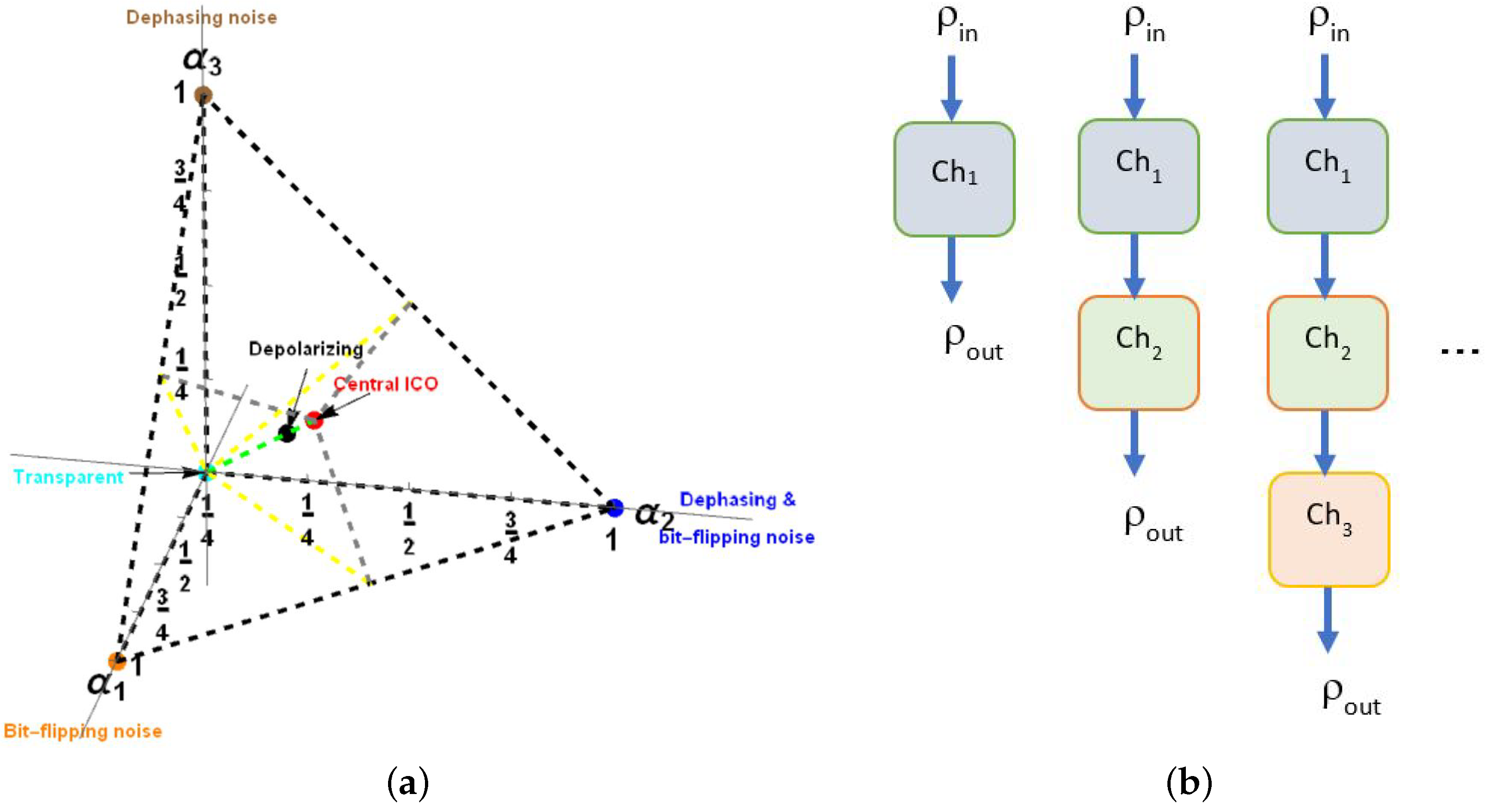
The latest formulas show the channel behaviour: if ${\alpha }_0=1,{\alpha }_i=0,i=1,2,3$ we have a transparent channel. Otherwise, if ${\alpha }_i=\frac{1}{4},i=0,1,2,3$, the channel is totally depolarizing. Other syndromes as Bit-Flipping (BFN) and Dephasing (DN) noises emerge when just one of ${\alpha }_i\ne 0,i=1,2,3$. Figure 2a [11], shows a graphical representation constructed for this type of channels on the $({\alpha }_1,{\alpha }_2,{\alpha }_3)$-space (considering that ${\alpha }_0=1-{\sum }_{i=1}^3{\alpha }_i$), together with the most emblematic ones. In the corners, BFN (${\alpha }_1=1$) and DN (${\alpha }_3=1$) channels, and their combination (${\alpha }_2=1$). Central ICO is a notable channel in the context of Indefinite Causal Order (ICO), which will be discussed in the next section [11].

2.4. QFI for Pauli Channels in the Bloch Representation

QFI for Pauli channels has been studied inclusively for its extension to larger systems [23], setting certain conditions to afford QPE efficiently, thus providing a theoretical framework for the parameter estimation analysis. Together, a protocol for the QPE on Pauli channels has been introduced [24]. In the current approach, we will provide quantitative outcomes about QPE for such channels with dimension $d=2$, thus characterizing them under specific composed arrangements. An important outcome for the current development is the existence of easier expressions for QFI when $\rho$ is expressed in the Bloch representation (such AN expression is in fact generalizable for higher dimensions than $d=2$ used for qubits). It could be expressed as [14,25,26]:

$$\begin{array}{c}\hfill {\mathcal{F}}_{ab}\left({\rho }_{\overrightarrow{n}}\right)=\left\{\begin{array}{cc}\left({\partial }_a\overrightarrow{n}\right)·\left({\partial }_b\overrightarrow{n}\right)+\frac{(\overrightarrow{n}·{\partial }_a\overrightarrow{n})(\overrightarrow{n}·{\partial }_b\overrightarrow{n})}{1-|\overrightarrow{n}{|}^2},\hfill & |\overrightarrow{n}|\ne 1\left(\mathrm{mixed}\mathrm{states}\right)\hfill \\ \left({\partial }_a\overrightarrow{n}\right)·\left({\partial }_b\overrightarrow{n}\right),\hfill & |\overrightarrow{n}|=1\left(\mathrm{pure}\mathrm{states}\right)\hfill \end{array}\right.\end{array}$$

(11)

Note $\overrightarrow{n}=|\overrightarrow{n}|\widehat{n}$, with: $\widehat{n}=(sin\theta cos\varphi ,sin\theta sin\varphi ,cos\theta )$, being $\theta ,\varphi$ the angles of the state representation on the Bloch ball. In addition, in our case of interest ${\partial }_a$ represents the partial derivative with respect the parameter a within $\overrightarrow{n}$. Particularly, parameter a appears as a result of the modification from ${\overrightarrow{n}}_{\mathrm{input}}$ into ${\overrightarrow{n}}_{\mathrm{ouput}}$ through a quantum channel. The last expression notably eases the calculation of QFI for the cases we are interested in the current development. It reduces to analyse the transition ${\overrightarrow{n}}_{\mathrm{input}}\to {\overrightarrow{n}}_{\mathrm{ouput}}$ through the quantum channel. When channels obey the rule $n_i^{\prime }=n_i{f}_i$, then the QFI for the output state fulfills:

$$\begin{array}{c}\hfill {\mathcal{F}}_{ab}\left({\rho }_{{\overrightarrow{n}}^{\prime }}\right)=\left\{\begin{array}{cc}\sum _{i=1}^3{n}_i^2\left({\partial }_a{f}_i\right)\left({\partial }_b{f}_i\right)+\frac{\left({\sum }_{i=1}^3{n}_i{\partial }_a{f}_i\right)\left({\sum }_{j=1}^3{n}_j{\partial }_b{f}_j\right)}{1-{\sum }_{i=1}^3{n}_i^2{f}_i^2},\hfill & |\overrightarrow{n}|\ne 1\left(\mathrm{mixed}\mathrm{states}\right)\hfill \\ \sum _{i=1}^3{n}_i^2\left({\partial }_a{f}_i\right)\left({\partial }_b{f}_i\right),\hfill & |\overrightarrow{n}|=1\left(\mathrm{pure}\mathrm{states}\right)\hfill \end{array}\right.\end{array}$$

(12)

3. Sequential and Indefinite Causal Order Arrangements of Pauli Channels

In the current section, we will analyse the behaviour of two new types of channel arrangements integrated by identical single Pauli channels: sequential and ICO. In both cases, we get the resultant form factors, which will be important to get the QFI for each case. For ICO arrangement, we develop a more complete approach than that presented in [11] to reach easier and comprehensive expressions for the output state in an ICO arrangement of Pauli channels. Our final objective is to analyse, through of comprehensive formulas for ${\rho }_{\mathrm{out}}$, the better schemes for QPE among single, sequential, and ICO arrangements through the entire Pauli channels parameter region.

3.1. Sequential Pauli Channels

A sequential application of any fixed Pauli channel has been presented in [11]. Thus, considering a set of n redundant identical noisy channels as a composition of the Formula (8):

$$({◯}_n\Lambda )\left[\rho \right]\equiv \Lambda [\Lambda [\dots \Lambda \left[\rho \right]\dots ]]=\sum _{i_1,\dots ,i_n=0}^3{\alpha }_{i_1}\cdots {\alpha }_{i_n}{\sigma }_{i_n}\cdots {\sigma }_{i_1}\rho {\sigma }_{i_1}\cdots {\sigma }_{i_n}$$

(13)

A representation of such process is illustrated in Figure 2b, where ${\rho }_{\mathrm{in}}=\rho$ and ${\rho }_{\mathrm{out}}=({◯}_n\Lambda )\left[\rho \right]$. Thus, an increasing number of channels ${\mathrm{Ch}}_1,{\mathrm{Ch}}_2,\cdots$ are applied to ${\rho }_{\mathrm{in}}$. For the last expression, based on outcome (10), we get:

$$({◯}_n\Lambda )\left[{\rho }_{\overrightarrow{n}}\right]=\frac{1}{2}({\sigma }_0+{\overrightarrow{n}}^{\left(n\right)}·\overrightarrow{\sigma }),\mathrm{with}:n_i^{\left(n\right)}=n_i{(1-2(n_j+n_k))}^n=n_i{f}_i^n$$

(14)

where $i,j,k$ is a cyclic permutation of $1,2,3$. We note that the behaviour of $\rho$ for each sequential channel depends jointly on the input state, as well as the channel’s parameters. Particularly, if $f_i<0$, it inverts repeatedly the direction of $\overrightarrow{n}$.

In this subsection, we are interested on the QFI for a noisy Pauli channel as depicted in (8), with its behaviour characterized by the parameters $({\alpha }_1,{\alpha }_2,{\alpha }_3)$ and the probe pure state $\rho =|\psi \rangle \langle \psi |$, with $|\psi \rangle =cos\frac{\theta }{2}|0\rangle +e^{i\varphi }sin\frac{\theta }{2}|1\rangle$. The goal is to analyse the CRB for the estimation of such set of parameters. Initially, for simplicity and as introductory analysis, we will consider the simpler case ${\alpha }_1={\alpha }_2={\alpha }_3\equiv p,0\le p\le \frac{1}{3}$ to avoid complex expressions involving the whole set of parameters. Such channels are located in the central straight line in the parametric space connecting the transparent and central ICO channels. Some of those states correspond to the inversion of the states in the Bloch ball if $2({\alpha }_0+{\alpha }_i)-1=1-4p<0$ in (10), then $\frac{1}{3}\ge p>\frac{1}{4}$. Then, it surpasses the depolarizing channel in $p=\frac{1}{4}$ doing that redundant applications converge to the depolarizing channel.

3.2. Pauli Channels under Indefinite Causal Order

Several approaches have proposed the use of coherently superposed noisy channels to improve the QPE [27]. ICO arrangements state the possibility to introduce such a kind of coherent superposition. Using previous developments for the expressions of ICO arrangements [8,9], such a scheme has been analysed for the quantum switch [28,29] with positive and remarkable outcomes for a single parameter, exploiting previous works in QPE around the depolarizing channel [30,31]. In the current approach, we deal with a wider analysis of channels than the depolarizing one but restricted to the qubit case ($d=2$).

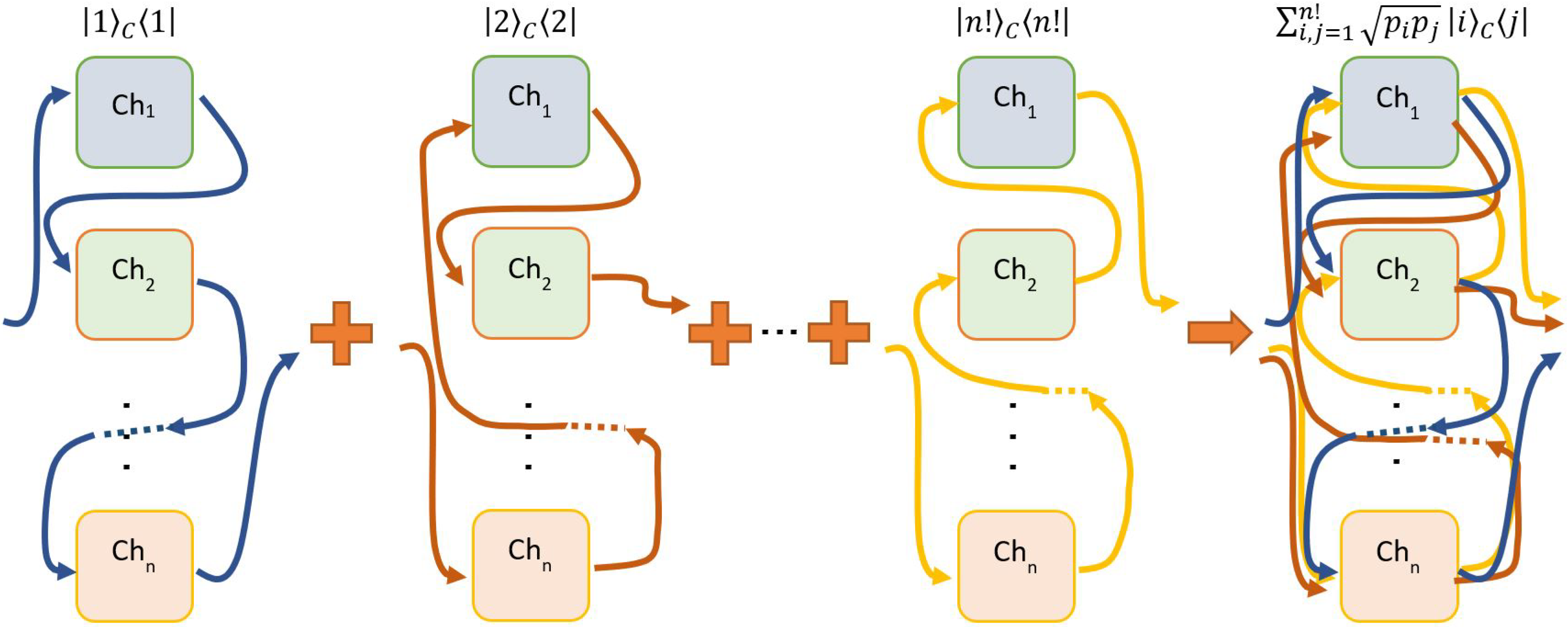
In [11], it has been developed the analysis for the ICO arrangement of Pauli channels. There, applying n channels in a superposition of causal orders, we get $n!$ possible combinations of them. A quantum control state with the same number of dimensions as channels combinations (being $|1\rangle$ the normal sequential order of channels ${\mathrm{Ch}}_1,{\mathrm{Ch}}_2,\dots ,{\mathrm{Ch}}_n$) addresses the causal order:

$${\rho }_C=(\sum _{i=1}^{n!}\sqrt{q_i}|i{\rangle }_C)(\sum _{j=1}^{n!}\sqrt{q_j}\langle j{|}_C)=\sum _{i,j=1}^{n!}\sqrt{q_i{q}_j}|i{\rangle }_C\langle j|$$

(15)

Figure 3 exhibits the causal orders combinations previously depicted, together with their associated control states. Thus, a definite causal order of communication channels ${\mathrm{Ch}}_{i_1},{\mathrm{Ch}}_{i_2},\dots ,{\mathrm{Ch}}_{i_n}$ could be understood as one generated by the element ${\pi }_k\in {\Sigma }_n$ in the symmetric group of permutations ${\Sigma }_n$ on the sequential ordered arrangement. The use of such a control will introduce entanglement between it and the main system used as a state probe for the QPE problem. The use of an entangled system to improve the estimation has been afforded previously [32].

3.2.1. Combinatoric Approach to the Output State Expression in Terms of Kraus Operators for ICO

Such group element will be understood having the following effect on the set of n single channel Kraus operators:

$$\begin{array}{c}\hfill {\pi }_k=\left(\begin{array}{cccc}{C}_{i_1}& C_{i_2}& \cdots & C_{i_n}\\ C_{i_{j_1}}& C_{i_{j_2}}& \cdots & C_{i_{j_n}}\end{array}\right)\to {\pi }_k(K_{i_1}{K}_{i_2}\cdots K_{i_n})=K_{i_{j_1}}{K}_{i_{j_2}}\cdots K_{i_{j_n}}\end{array}$$

(16)

It will be symbolically associated with the control state ${|k\rangle }_c$. The corresponding global Kraus operators $W_{i_1,i_2,\dots ,i_n}$ for the whole channel will be [5]:

$$W_{i_1,i_2,\dots ,i_n}=\sum _{k=1}^{n!}{\pi }_k(K_{i_1}{K}_{i_2}\dots K_{i_n})\otimes {|k\rangle }_c\langle k|$$

(17)

We will sometimes omit the tensor product symbol ⊗ in spite of simplicity. Then, the output for the $n$—channels in ICO becomes [11]:

$$\begin{array}{ccc}\hfill & & {\Lambda }^n\left[\rho \otimes {\rho }_c\right]=\sum _{i_1,i_2,\dots ,i_n}{W}_{i_1,i_2,\dots ,i_n}\rho \otimes {\rho }_c{\left(W_{i_1,i_2,\dots ,i_n}\right)}^{†}\hfill \\ & & =\sum _{i_1,\dots ,i_n}\left(\sum _k{\pi }_k\left(K_{i_1}\dots K_{i_n}\right)|k\rangle \langle k|\right)\rho \otimes {\rho }_c{\left(\sum _{k^{\prime }}{\pi }_{k^{\prime }}\left(K_{i_1}\dots K_{i_n}\right)|k^{\prime }\rangle \langle k^{\prime }|\right)}^{†}\hfill \end{array}$$

(18)

$$\begin{array}{ccc}& & =\sum _{\begin{array}{c}{i}_1,\dots ,i_n\\ k,k^{\prime }\end{array}}\prod _{j=1}^n{\alpha }_{i_j}\sqrt{q_k{q}_{k^{\prime }}}|k\rangle \langle k^{\prime }|\otimes {\pi }_k\left({\sigma }_{i_1}\cdots {\sigma }_{i_n}\right)\rho {\pi }_{k^{\prime }}^{†}\left({\sigma }_{i_1}\cdots {\sigma }_{i_n}\right)\hfill \end{array}$$

(19)

being $K_j=\sqrt{{\alpha }_j}{\sigma }_j$ as in the previous section. As in [11], Formula (18) becomes simpler using combinatorics together with the properties of Pauli operators. In fact, by noting that the sum in (19) involves all different values assigned to $i_1,i_2,\dots ,i_n$, after they are permuted as distinguishable objects by ${\pi }_k$ and ${\pi }_{k^{\prime }}$, it can be switched as [8]:

$$\begin{array}{c}\hfill \sum _{i_1=0}^3\sum _{i_2=0}^3\cdots \sum _{i_n=0}^3⟶\sum _{t_1=0}^n\sum _{t_2=0}^{n-t_1}\sum _{t_3=0}^{n-t_1-t_2}\sum _{p=1}^{n^{\prime }}\end{array}$$

(20)

with $t_j$ as the number of scripts in $i_1,i_2,\dots ,i_n$ equal to $j=0,1,2,3$ (then, $t_0=n-t_1-t_2-t_3$). The sum over p ranges on the distinguishable arrangements obtained with a fix number $t_j$ of operators ${\sigma }_j$ involved and obtained through a specific permutation ${\pi }_{k_p^{t_1,t_2,t_3}}$. It implies the permutations among identical operators in each one of the three groups ${\sigma }_1,{\sigma }_2,{\sigma }_3$ are indistinguishable. Additionally, $n^{\prime }=\frac{n!}{t_0!t_1!t_2!t_3!}$ is the total of different cases involved. Finally, (19) can be written as in [11]:

$$\begin{array}{ccc}\hfill {\Lambda }^n\left[\rho \otimes {\rho }_C\right]& =& \sum _k\sum _{k^{\prime }}\sqrt{q_k{q}_{k^{\prime }}}|k\rangle \langle k^{\prime }|\sum _{t_1=0}^n\sum _{t_2=0}^{n-t_1}\sum _{t_3=0}^{n-t_1-t_2}\prod _{j=0}^3{\alpha }_j^{t_j}\otimes \hfill \\ & & \sum _{p=1}^{n^{\prime }}{\pi }_k\left({\pi }_{k_p^{t_1,t_2,t_3}}\left({\sigma }_0^{t_0}{\sigma }_1^{t_1}{\sigma }_2^{t_2}{\sigma }_3^{t_3}\right)\right)\rho {\left({\pi }_{k^{\prime }}\left({\pi }_{k_p^{t_1,t_2,t_3}}\left({\sigma }_0^{t_0}{\sigma }_1^{t_1}{\sigma }_2^{t_2}{\sigma }_3^{t_3}\right)\right)\right)}^{†}\hfill \end{array}$$

(21)

Thus, (21) sets an easier formula for ${\rho }_{\mathrm{out}}={\Lambda }^n\left[\rho \otimes {\rho }_c\right]$ just including a definite number of sums. In addition, the transmitted state is practically separated from the control state.

3.2.2. Simplification for the Output State Expression Using Its Combinatoric Properties

Considering the properties of Pauli operators’ algebra, we note that both permutation terms beside $\rho$ in (21) are equal until an algebraic sign. Additionally, each one belongs to the set $\left\{{\sigma }_j\right|j=0,1,2,3\}$. Due if all $t_1,t_2,t_3$ are altogether even or odd ($t_0$ is meaningfulness) then ${\sigma }_0^{t_0}{\sigma }_1^{t_1}{\sigma }_2^{t_2}{\sigma }_3^{t_3}$ becomes proportional to ${\sigma }_0$. In addition, if $t_j$ is the only even or odd among $t_1,t_2,t_3$, then such product becomes proportional to ${\sigma }_j$. In this way, (21) becomes a mixed state obtained from the syndromes ${\sigma }_j\rho {\sigma }_j,j=0,1,2,3$ altogether entangled with the control state. As it was stated in [11], the most complex issue in (22) is the global sign for each term.

Because the control state is still included in our output state, we can analyse the QFI together, or otherwise to make a convenient projective measurement on certain control state $|{\psi }_m\rangle$. In fact, it is not strictly necessary, because QFI can be still analysed on the entire system as it was performed with the depolarizing channel [28]. In such a case, sometimes, specific forms for the control state are introduced, particularly the so-called cyclic arrangement [10]. Otherwise, certain advantages have been noticed using post-selection [33] inducing a selection stochastically. In such a case, an adequate basis is selected to perform a measurement for the control state: $\mathcal{B}=\left\{\right|{\psi }_{M_i}\rangle |i=1,2,\dots ,n!\}$. In such a basis, it is expected to find a privileged state $|{\psi }_m\rangle \in \mathcal{B}$ improving the effects of ICO [11]. Thus, in that case we get the post-measurement state:

$$\begin{array}{ccc}\hfill {\Lambda }_m^n\left[\rho \right]& =& \frac{\langle {\psi }_m\left|{\Lambda }^n\left[\rho \otimes {\rho }_c\right]\right|{\psi }_m\rangle }{{\mathcal{P}}_m}\hfill \\ & =& \frac{1}{{\mathcal{P}}_m}\sum _{k,k^{\prime }}\sqrt{q_k{q}_{k^{\prime }}}\langle {\psi }_m|k\rangle \langle k^{\prime }|{\psi }_m\rangle \sum _{t_1=0}^n\sum _{t_2=0}^{n-t_1}\sum _{t_3=0}^{n-t_1-t_2}\prod _{j=0}^3{\alpha }_j^{t_j}·\hfill \\ & & \sum _{p=1}^{n^{\prime }}{\pi }_k\left({\pi }_{k_p^{t_1,t_2,t_3}}\left({\sigma }_0^{t_0}{\sigma }_1^{t_1}{\sigma }_2^{t_2}{\sigma }_3^{t_3}\right)\right)\rho {\left({\pi }_{k^{\prime }}\left({\pi }_{k_p^{t_1,t_2,t_3}}\left({\sigma }_0^{t_0}{\sigma }_1^{t_1}{\sigma }_2^{t_2}{\sigma }_3^{t_3}\right)\right)\right)}^{†}\hfill \end{array}$$

(22)

$$\begin{array}{ccc}\hfill {\mathcal{P}}_m& =& \mathrm{Tr}(\langle {\psi }_m|{\Lambda }^n\left[\rho \otimes {\rho }_c\right]|{\psi }_m\rangle )\hfill \end{array}$$

(23)

where ${\mathcal{P}}_m$ is the success probability of measurement. Considering the Bloch representation of $\rho$ (9), we could note that:

(1)

In the calculation of ${\mathcal{P}}_m$ (23), only the term involving ${\sigma }_0$ in the Bloch expression of $\rho$ contributes it because $\mathrm{Tr}\left({\sigma }_i\right)=0,i=1,2,3$ in the further terms, thus giving a simpler expression for it. It implies that the first term in ${\Lambda }_m^n\left[\rho \right]$ (22) coming from ${\sigma }_0$ in $\rho$ gives precisely $\frac{{\sigma }_0}{2}$.

(2)

Last affirmation also arises from the fact that each sum at the end of ${\Lambda }_m^n\left[\rho \right]$ has the same terms on each side of $\rho$, then because the properties of the algebra of ${\sigma }_{\alpha },\alpha =0,1,2,3$ (commuting or anti-commuting) terms involving ${\sigma }_0,{\sigma }_1,{\sigma }_2,{\sigma }_3$ evolves into themselves, possibly with a different sign.

(3)

In the following, we will express the last sum in ${\Lambda }_m^n\left[\rho \right]$ as $S_{l_{k,k^{\prime }}}^{p,\left\{t_i\right\}}{\sigma }_l\equiv {\sum }_{p=1}^{n^{\prime }}{\pi }_k\left({\pi }_{k_p^{t_1,t_2,t_3}}\left({\sigma }_0^{t_0}{\sigma }_1^{t_1}{\sigma }_2^{t_2}{\sigma }_3^{t_3}\right)\right){\sigma }_l{\left({\pi }_{k^{\prime }}\left({\pi }_{k_p^{t_1,t_2,t_3}}\left({\sigma }_0^{t_0}{\sigma }_1^{t_1}{\sigma }_2^{t_2}{\sigma }_3^{t_3}\right)\right)\right)}^{†}$, being $S_{l_{k,k^{\prime }}}^{p,\left\{t_i\right\}}$ the sign emerging from the Pauli operators algebra.

Then, based on the last facts, we can write:

$$\begin{array}{ccc}\hfill {\Lambda }_m^n\left[\rho \right]& =& \frac{1}{2}\left({\sigma }_0+\sum _{l=1}^3{n}_l{f}_l^{\mathrm{ICO}}{\sigma }_l\right)\hfill \end{array}$$

(24)

$$\begin{array}{ccc}\hfill f_l^{\mathrm{ICO}}& =& \frac{1}{{\mathcal{P}}_m}\sum _{k,k^{\prime }}\sqrt{q_k{q}_{k^{\prime }}}\langle {\psi }_m|k\rangle \langle k^{\prime }|{\psi }_m\rangle \sum _{t_1=0}^n\sum _{t_2=0}^{n-t_1}\sum _{t_3=0}^{n-t_1-t_2}\prod _{j=0}^3{\alpha }_j^{t_j}·\sum _{p=1}^{n^{\prime }}{S}_{l_{k,k^{\prime }}}^{p,\left\{t_i\right\}}\hfill \end{array}$$

(25)

$$\begin{array}{ccc}\hfill S_{l_{k,k^{\prime }}}^{p,\left\{t_i\right\}}{\sigma }_l& =& {\pi }_k\left({\pi }_{k_p^{t_1,t_2,t_3}}\left({\sigma }_0^{t_0}{\sigma }_1^{t_1}{\sigma }_2^{t_2}{\sigma }_3^{t_3}\right)\right){\sigma }_l\left({\pi }_{k^{\prime }}{\left({\pi }_{k_p^{t_1,t_2,t_3}}\left({\sigma }_0^{t_0}{\sigma }_1^{t_1}{\sigma }_2^{t_2}{\sigma }_3^{t_3}\right)\right)}^{†}\right)\hfill \end{array}$$

(26)

$$\begin{array}{ccc}\hfill {\mathcal{P}}_m& =& \sum _{k,k^{\prime }}\sqrt{q_k{q}_{k^{\prime }}}\langle {\psi }_m|k\rangle \langle k^{\prime }|{\psi }_m\rangle \sum _{t_1=0}^n\sum _{t_2=0}^{n-t_1}\sum _{t_3=0}^{n-t_1-t_2}\prod _{j=0}^3{\alpha }_j^{t_j}\sum _{p=1}^{n^{\prime }}{S}_{0_{k,k^{\prime }}}^{p,\left\{t_i\right\}}\hfill \end{array}$$

(27)

It shows that ${\mathcal{P}}_m$ is independent from the input state $\overrightarrow{n}$. In fact, the complexity of the above expression is centered on $S_{l_{k,k^{\prime }}}^{p,\left\{t_i\right\}}{\sigma }_l$. The nature of signs $S_{{\alpha }_{k,k^{\prime }}}^{p,\left\{t_i\right\}},\alpha =0,1,2,3$ has been discussed in [11]. Here, we will extend the outcomes obtained in [11] for the frontal face (${\alpha }_0=0$). There, the sums on p and $k,k^{\prime }$ were inverted, concretely:

$$\begin{array}{ccc}\hfill {\mathcal{P}}_m{f}_l^{\mathrm{ICO}}{\sigma }_l& =& \sum _{t_1=0}^n\sum _{t_2=0}^{n-t_1}\sum _{t_3=0}^{n-t_1-t_2}\prod _{j=0}^3{\alpha }_j^{t_j}·\sum _{p=1}^{n^{\prime }}{\mathcal{L}}_{{\psi }_m}{\sigma }_l{\mathcal{L}}_{{\psi }_m}^{†}\hfill \\ & & \mathrm{where}:{\mathcal{L}}_{{\psi }_m}=\sum _k\sqrt{q_k}\langle {\psi }_m|k\rangle {\pi }_k\left({\pi }_{k_p^{t_1,t_2,t_3}}\left({\sigma }_0^{t_0}{\sigma }_1^{t_1}{\sigma }_2^{t_2}{\sigma }_3^{t_3}\right)\right)\hfill \end{array}$$

(28)

as in [11], we note that taking a fix set for $t_0,t_1,t_2,t_3$, then ${\sigma }_0^{t_0}{\sigma }_1^{t_1}{\sigma }_2^{t_2}{\sigma }_3^{t_3}={\sigma }_1^{t_1}{\sigma }_2^{t_2}{\sigma }_3^{t_3}$ evolves proportional to some ${\sigma }_h$ in agreement with the rule:

$$\begin{array}{c}\hfill h=\left\{\begin{array}{cc}0,\hfill & t_i,i=1,2,3\mathrm{are}\mathrm{all}\mathrm{even}\mathrm{or}\mathrm{odd}\hfill \\ \kappa ,\hfill & t_{\kappa }\in \left\{t_i\right|i=1,2,3\}\mathrm{is}\mathrm{the}\mathrm{only}\mathrm{even}\mathrm{or}\mathrm{odd}\hfill \end{array}\right.\end{array}$$

(29)

In particular, factors of i arising in each term of ${\mathcal{L}}_{{\psi }_m}$ should be the same once the operators were sort to be simplified. Then, those factors will cancel each one with another in each side ${\mathcal{L}}_{{\psi }_m},{\mathcal{L}}_{{\psi }_m}^{†}$ because they are independent from the order of operators.

3.2.3. Operative Optimal Expressions for the Output State Expression under ICO

Thus, for each set $t_0,t_1,t_2,t_3$, the operator ${\sigma }_h{\sigma }_l{\sigma }_h$ emerges (after evolving to ${\sigma }_l$) together with a squared sum of terms with signs $s_k^{p,\left\{t_i\right\}}$ obtained as a result of the sorting of operators into ${\sigma }_0^{t_0}{\sigma }_1^{t_1}{\sigma }_2^{t_2}{\sigma }_3^{t_3}$:

$$\begin{array}{ccc}\hfill {\mathcal{P}}_m{f}_l^{\mathrm{ICO}}{\sigma }_l& =& \sum _{t_1=0}^n\sum _{t_2=0}^{n-t_1}\sum _{t_3=0}^{n-t_1-t_2}\prod _{j=0}^3{\alpha }_j^{t_j}·{\sigma }_h{\sigma }_l{\sigma }_h\sum _{p=1}^{n^{\prime }}{\left|{\mathcal{C}}_{p,\left\{t_i\right\}}\right|}^2\hfill \\ & & \mathrm{where}:{\mathcal{C}}_{p,\left\{t_i\right\}}=\sum _k\sqrt{q_k}\langle {\psi }_m|k\rangle s_k^{p,\left\{t_i\right\}}\hfill \end{array}$$

(30)

signs $s_k^{p,\left\{t_i\right\}}$ depends on the specific order of operators in ${\pi }_k\left({\pi }_{k_p^{t_1,t_2,t_3}}\left({\sigma }_0^{t_0}{\sigma }_1^{t_1}{\sigma }_2^{t_2}{\sigma }_3^{t_3}\right)\right)$ by evolving into ${\sigma }_0^{t_0}{\sigma }_1^{t_1}{\sigma }_2^{t_2}{\sigma }_3^{t_3}$.

As it was discussed in [34], ${\pi }_k\left({\pi }_{k_p^{t_1,t_2,t_3}}\left({\sigma }_0^{t_0}{\sigma }_1^{t_1}{\sigma }_2^{t_2}{\sigma }_3^{t_3}\right)\right)$ should be understood as the permutation of ${\sigma }_0^{t_0}{\sigma }_1^{t_1}{\sigma }_2^{t_2}{\sigma }_3^{t_3}$ into the $n^{\prime }=\frac{n!}{t_0!t_1!t_2!t_3!}$ ways. They could be arranged in different ways with a fix selection of $t_0,t_1,t_2,t_3$. Afterwards, $\left\{{\pi }_k\right\}$ performs a complete set of $n!$ permutations in the positions. Due to the terms $\sqrt{q_k}\langle {\psi }_m|k\rangle$ involved, there is not an apparent independence between p and k in general. Nevertheless, despite departing from a given p ordering, then each ${\pi }_k$ will give different signs $s_k^{p,\left\{t_i\right\}}$, because all possible permutations are considered and they uniformly differ from some sign with respect another $p^{\prime }$ value, then such sign could be factorized and it will disappear because the squaring. Thus, sums ${\mathcal{C}}_{p,\left\{t_i\right\}}$ could be considered independent of p, just ${\mathcal{C}}_{\left\{t_i\right\}}$ in the following, only introducing an $n^{\prime }$ factor (in fact, at this point it will be expected because signs are associated just to the ordering of each permutation into the final form ${\sigma }_0^{t_0}{\sigma }_1^{t_1}{\sigma }_2^{t_2}{\sigma }_3^{t_3}$). Clearly, ${\sigma }_h{\sigma }_l{\sigma }_h$ evolves into ${\sigma }_l$ depending on (29) and if $l,h$ are equal or different:

$$\begin{array}{ccc}\hfill {\sigma }_h{\sigma }_l{\sigma }_h& =& \left\{\begin{array}{cc}{\sigma }_l,\hfill & t_i,i=1,2,3\mathrm{are}\mathrm{all}\mathrm{even}\mathrm{or}\mathrm{odd}\mathrm{or}{t}_l\mathrm{is}\mathrm{the}\mathrm{only}\mathrm{even}\mathrm{or}\mathrm{odd}\hfill \\ -{\sigma }_l,\hfill & t_l\ne t_{\kappa }\mathrm{with}{t}_{\kappa }\in \left\{t_i\right|i=1,2,3\}\mathrm{is}\mathrm{the}\mathrm{only}\mathrm{even}\mathrm{or}\mathrm{odd}\hfill \end{array}\right.\hfill \\ & \equiv & {(-1)}^{{\Delta }_{l,h}}{\sigma }_l\hfill \end{array}$$

(31)

Following the same procedure, we can get a simplified expression for $f_l^{\mathrm{ICO}}$ and ${\mathcal{P}}_m$:

$$\begin{array}{ccc}\hfill f_l^{\mathrm{ICO}}& =& \frac{1}{{\mathcal{P}}_m}\sum _{t_1=0}^n\sum _{t_2=0}^{n-t_1}\sum _{t_3=0}^{n-t_1-t_2}\prod _{j=0}^3{\alpha }_j^{t_j}{(-1)}^{{\Delta }_{l,h}}{n}^{\prime }{\left|{\mathcal{C}}_{\left\{t_i\right\}}\right|}^2\hfill \end{array}$$

(32)

$$\begin{array}{ccc}\hfill {\mathcal{P}}_m& =& \sum _{t_1=0}^n\sum _{t_2=0}^{n-t_1}\sum _{t_3=0}^{n-t_1-t_2}\prod _{j=0}^3{\alpha }_j^{t_j}{n}^{\prime }{\left|{\mathcal{C}}_{\left\{t_i\right\}}\right|}^2\hfill \end{array}$$

(33)

Analysing $s_k^{p,\left\{t_i\right\}}$ as in [34], and considering that each operator term can be characterized by a string of integer numbers of ordered equal adjacent operators: $m_0^1,m_1^1,m_2^1,m_3^1,m_0^2,m_1^2,m_2^2,m_3^2,\dots ,m_3^s$. Being s the number of groups necessary for such description (as instance, ${\sigma }_0{\sigma }_2{\sigma }_2{\sigma }_1{\sigma }_0{\sigma }_3{\sigma }_2$ has $m_0^1=1,m_1^1=0,m_2^1=2,m_3^1=0,m_0^2=0,m_1^2=1,m_2^2=0,m_3^2=0,m_0^3=1,m_1^3=0,m_2^3=0,m_3^3=1,m_0^4=0,m_1^4=0,m_2^4=1,m_3^4=0$, thus $s=4$). Then, $m_i^j$ satisfies ${\sum }_{j=1}^s{m}_i^j=t_i$ and ${\sum }_{i=0}^3{\sum }_{j=1}^s{m}_i^j=N$. By moving each type of operators on the left to put them in order, first ${\sigma }_1$ then ${\sigma }_2$ (without leap ${\sigma }_2$ on ${\sigma }_1$) to carry out ${\sigma }_{j_1}{\sigma }_{j_2}\dots {\sigma }_{j_N}$ into ${\sigma }_0^{t_0}{\sigma }_1^{t_1}{\sigma }_2^{t_2}{\sigma }_3^{t_3}$, we note $s_k^{p,\left\{t_i\right\}}$ fulfills:

$$\begin{array}{ccc}\hfill s_k^{p,\left\{t_i\right\}}& =& {(-1)}^{{\Delta }_k^{p,\left\{t_i\right\}}}\hfill \\ & & \mathrm{with}:{\Delta }_k^{p,\left\{t_i\right\}}=\sum _{i=2}^s\sum _{j=1}^{i-1}{m}_1^i(m_2^j+m_3^j)+\sum _{i=2}^s\sum _{j=1}^{i-1}{m}_2^i{m}_3^j\hfill \end{array}$$

(34)

which provides an easier expression to get ${\Lambda }_m^n\left[\rho \right]$ ($f_l^{\mathrm{ICO}}$ and ${\mathcal{P}}_m$), and then QFI from (11). The last procedure summarized on Formulas (32)–(34) becomes a valuable outcome to get the expression of ${\Lambda }_m^n\left[\rho \right]$ in the Bloch representation for higher values of n. It still becomes also useful for the non-stochastic case ${\Lambda }^n[\rho \otimes {\rho }_C]$.

3.2.4. Stochastic Approaches and Some Privileged Measurements on the Control System

We have developed Formulas (32) and (33) as part of a stochastic procedure. Then, an intermediate measurement on the control system is performed to get a certain preferred state. If such a state is successfully obtained, the QPE process continues, if not, it should be begun again. More general expressions of such an approach could be recovered eliminating $|{\psi }_m\rangle$, leaving them in terms of an entangled state with the control. For the stochastic approach, there are lots of possibilities to set the control state together with $|{\psi }_m\rangle$. Proposed by [35] and analysed by [11], the following two states maximize the fidelity of (22) as function of the parity of n (suggesting the generation of a transparent channel on the frontal face of the space represented in Figure 2a):

$$\begin{array}{c}\hfill |{\psi }_m^{n,\pm }\rangle =\frac{1}{\sqrt{n!}}\sum _{k=0}^{n!-1}{(\pm 1)}^{\sigma \left({\pi }_k\right)}{|k\rangle }_C\end{array}$$

(35)

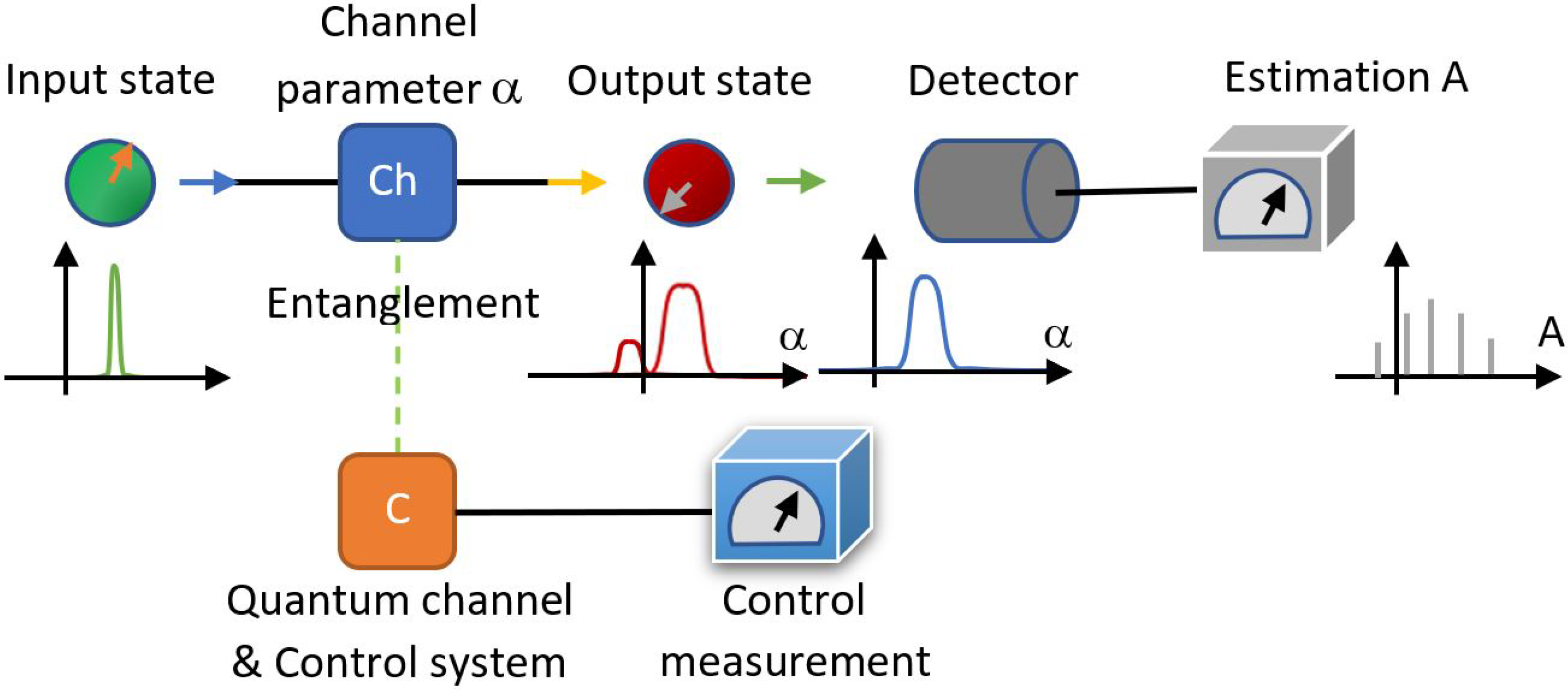
Here, $\sigma \left({\pi }_k\right)$ represents the parity of the permutation ${\pi }_k$, 0 for even or 1 for odd. In addition, $q_k$ could be selected evenly as $q_k=\frac{1}{n!}$. We will consider in our further development last post-measurement stochastic process using these states to analyse QFI in this work. Figure 4 shows the process, where an intermediate measurement on the control system produces a specific state to be analysed under QPE of the channel parameters. When the control state is measured as the preferred one, then the QPE process is continued, otherwise repeated. In the first case:

$$\begin{array}{c}\hfill {\mathcal{C}}_{\left\{t_i\right\}}^{\pm }\equiv \frac{1}{n!}\sum _k{(-1)}^{{\Delta }_k^{p,\left\{t_i\right\}}}{(\pm 1)}^{\sigma \left({\pi }_k\right)}\end{array}$$

(36)

In [11], it has been studied the fidelity on the frontal face of region in Figure 2. Note that the analysis conducted here extends the outcomes on the entire parametric region of Pauli channels. It is important be aware that sign generated by ${\Delta }_k^{p,\left\{t_i\right\}}$ is associated with the simplification of permutations involving Pauli operators in the Kraus operators expressions for channels under ICO, where factors ${\sigma }_0$ could be dropped. However, signs introduced by the signature $\sigma \left({\pi }_k\right)$ of each permutation consider the original objects with n factors including ${\sigma }_0$.

Following the analysis in [11], we conveniently will associate the signature election ± in ${\mathcal{C}}_{\left\{t_i\right\}}^{\pm }$ as a function of n, it means ${(\pm 1)}^{\sigma \left({\pi }_k\right)}={(-1)}^{n\sigma \left({\pi }_k\right)}$. Formulas (32)–(36) contain a simplified procedure to get expressions for $f_l^{\mathrm{ICO}}$ and ${\mathcal{P}}_m$ depicting the output state emerging from the Pauli channels under ICO. Still, those expressions should be addressed computationally to manage their complex analytical form. Nevertheless, this approach improves that one given in [11] by extending the analysis to the entire Pauli channels parametric space, not only to the frontal face.

4. QFI for Sequential and Indefinite Causal Order Arrangements of Pauli Channels

In the current section, we will explore concrete expressions for QFI for the sequential and ICO channels settled before, particularly when the Bloch representation is used. In parallel, we develop an previous insight for the CRB with a characteristic single parameter analysed in terms of QFI function $\mathcal{F}=\frac{1}{\mathcal{V}}$ to get a single view for the behaviour of the CRB in the multi-parametric case.

4.1. QFI Behavior as Parameter Estimator for Pauli Channels in a Sequential Arrangement

Taking the expression (14), QFI could be expressed in terms of $f_i$ factors, also considering that ${\partial }_a{f}_i=-2(1-{\delta }_{ia})\equiv -2{\tilde{\delta }}_{ia}$, being ${\delta }_{ij}$ the Kronecker delta. In this case, ${\partial }_a\equiv {\partial }_{{\alpha }_a}$ in brief. Then:

$$\begin{array}{ccc}\hfill {\mathcal{F}}_{ab}\left(({◯}_n\Lambda )\left[{\rho }_{\overrightarrow{n}}\right]\right)& =& 4n^2\sum _{i=1}^3{n}_i^2{f}_i^{2(n-1)}{\tilde{\delta }}_{ia}{\tilde{\delta }}_{ib}\hfill \\ & +& \left\{\begin{array}{cc}\frac{4n^2\left({\sum }_{i=1}^3{n}_i^2{f}_i^{2n-1}{\tilde{\delta }}_{ia}\right)\left({\sum }_{j=1}^3{n}_j^2{f}_j^{2n-1}{\tilde{\delta }}_{ja}\right)}{1-{\sum }_{i=1}^3{n}_i^2{f}_i^{2n}},\hfill & |{\overrightarrow{n}}_{\mathrm{output}}|<1\left(\mathrm{mixed}\mathrm{states}\right)\hfill \\ 0,\hfill & |{\overrightarrow{n}}_{\mathrm{output}}|=1\left(\mathrm{pure}\mathrm{states}\right)\hfill \end{array}\right.\hfill \end{array}$$

(37)

Such an expression still could become complex when $f_i$ is expressed in terms of the set $\left\{{\alpha }_a\right|a=1,2,3\}$ and ${\overrightarrow{n}}_{\mathrm{input}}=(n_1,n_2,n_3)=\left|{\overrightarrow{n}}_{\mathrm{input}}\right|(sin\theta cos\varphi ,sin\theta sin\varphi ,cos\theta )$, particularly if a further optimization process should be performed in terms of $\theta ,\varphi$ for each set $\left\{{\alpha }_a\right|a=1,2,3\}$. Unfortunately, for each channel defined by each $\left\{{\alpha }_a\right|a=1,2,3\}$, QFI depends on each input state $|{\overrightarrow{n}}_{\mathrm{input}}|,\theta ,\varphi$, thus setting test states to optimally reducing the Cramér–Rao bound.

Under certain circumstances, channels could be simplified to avoid the large number of parameters considering the simplification ${\alpha }_i=p\in [0,\frac{1}{3}],i=1,2,3$. In [34], such an approach demonstrated that the fidelity for an imperfect teleportation channel under sequential and ICO arrangements becomes independent of the teleported state. We can try to get then a simpler expression for (37) in such simplified approach. In such a case, there is just one parameter characterizing the channel, then $\mathcal{F}$ becomes a scalar:

$$\begin{array}{ccc}\hfill \mathcal{F}\left(({◯}_n\Lambda )\left[{\rho }_{\overrightarrow{n}}\right]\right)& =& \left\{\begin{array}{cc}\frac{16n^2{\left|{\overrightarrow{n}}_{\mathrm{input}}\right|}^2{(1-4p)}^{2(n-1)}}{1-|{\overrightarrow{n}}_{\mathrm{input}}{|}^2{(1-4p)}^{2n}},\hfill & |{\overrightarrow{n}}_{\mathrm{output}}|<1\left(\mathrm{mixed}\mathrm{states}\right)\hfill \\ 16n^2{\left|{\overrightarrow{n}}_{\mathrm{input}}\right|}^2{(1-4p)}^{2(n-1)},\hfill & |{\overrightarrow{n}}_{\mathrm{output}}|=1\left(\mathrm{pure}\mathrm{states}\right)\hfill \end{array}\right.\hfill \end{array}$$

(38)

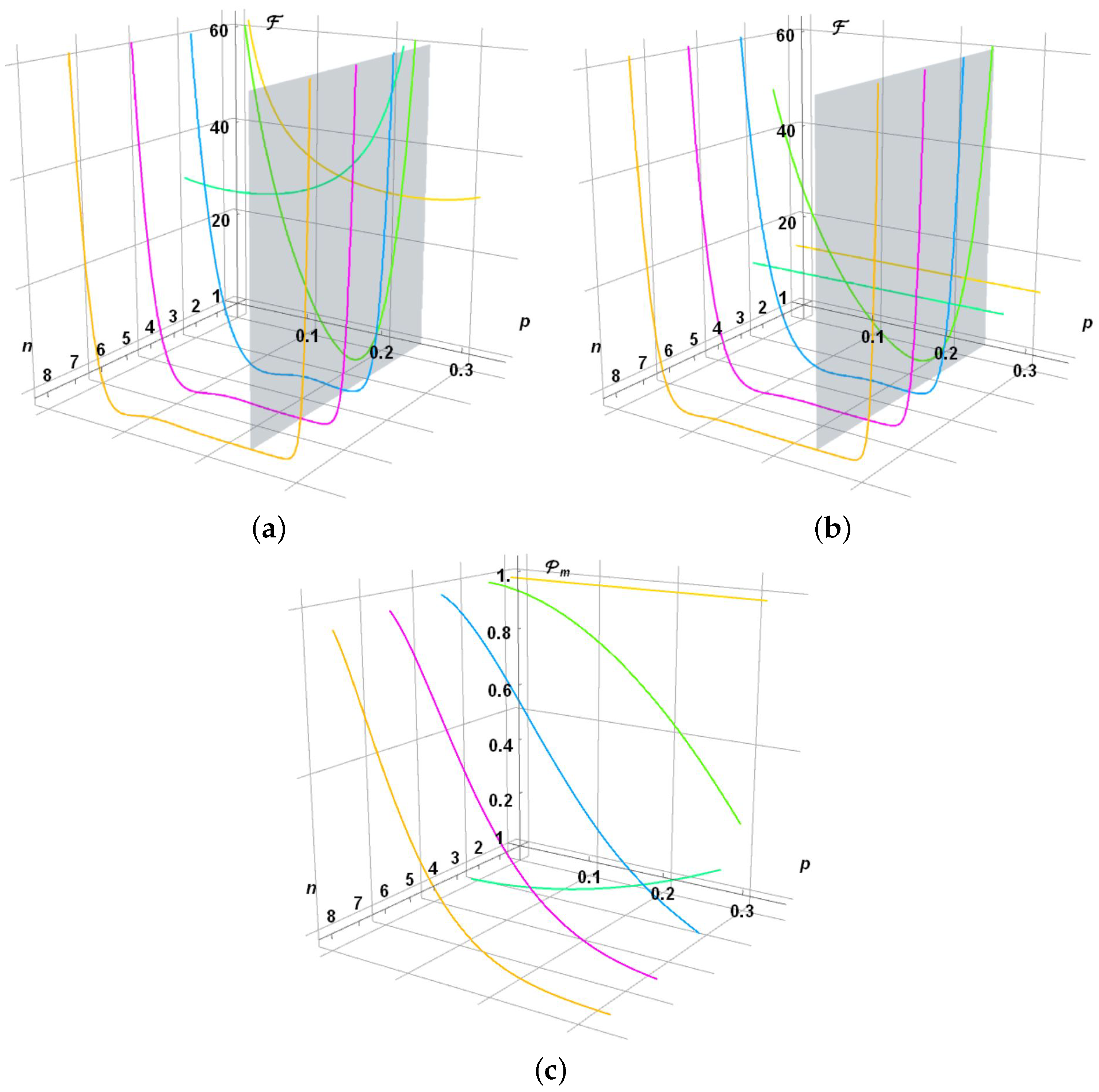
and we get it also independent from $\overrightarrow{n}$, it means from the input state ${\rho }_{\mathrm{input}}$ (with exception of $|{\overrightarrow{n}}_{\mathrm{input}}|$). Figure 5 shows the behaviour for QFI for n sequential channels $\mathcal{F}\left(({◯}_n\Lambda )\left[{\rho }_{\overrightarrow{n}}\right]\right)$ as function of $p\in [0,\frac{1}{3}]$. Figure 5a shows the behaviour for mixed output states, instead Figure 5b does for pure ones. Nevertheless, the first plot becomes more meaningful because channels commonly produce mixed states. Such behaviour of $\mathcal{F}$ becomes discontinuous, which has been analysed in several works [36,37]. We restricted the analysis there for initial input pure states $|{\overrightarrow{n}}_{\mathrm{input}}|=1$. In agreement with (6) for one channel parameter, $\mathrm{var}\left(p\right)\ge \frac{1}{\mathcal{F}}={\mathcal{V}}_{\mathrm{h}}={\mathcal{V}}_{\mathrm{s}}$. Then, we are avoiding the lower values for $\mathcal{F}$ where the QPE becomes worse.

Differences for $\mathcal{F}$ in Figure 5a,b are only notable for low values of n. In addition, $\mathcal{F}\left(({◯}_n\Lambda )\left[{\rho }_{\overrightarrow{n}}\right]\right)$ becomes almost zero on an extended and larger region of $[0,\frac{1}{3}]$ while n grows, thus indicating that ${\mathcal{V}}_{\mathrm{h}}$ is higher, then avoiding the prediction of the parameter value p by stacking identical channels (the reason should become clear, by stacking the channels, we are reaching the depolarizing channel). Mixed states become better test states for $n=1$. Gray planes remark $p=\frac{1}{4}$, the zone where the totally depolarizing channel is, matching with the minimum QFI (the maximum ${\mathcal{V}}_{\mathrm{h}}$) as it is evident from (38). Such minimum matches between pure and mixed states being equal to $\mathcal{F}\left(({◯}_n\Lambda )\left[{\rho }_{\overrightarrow{n}}\right]\right)=0$, a complete ignorance of parameter with ${\mathcal{V}}_{\mathrm{h}}^{1/2}\to \infty$. For the transparent channel $p=0$ and input pure states, $\mathcal{F}\left(({◯}_n\Lambda )\left[{\rho }_{\overrightarrow{n}}\right]\right)=16n^2$, then ${\mathcal{V}}_{\mathrm{h}}^{1/2}=\frac{1}{4n}$ (considering output pure states expression because in this case the output states remain pure). It implies a possible advantage for the sequential application of channels. ICO channel, $p=\frac{1}{3}$, does not show an advantage in this scheme (input pure state) because ${\mathcal{V}}_{\mathrm{h}}^{1/2}=\frac{{(3^{2n}-1)}^{1/2}}{12n}$ (considering an output mixed state).

4.2. Behavior of QFI as Parameter Estimator for Pauli Channels in an ICO Arrangement

Developing the expression (11) together with Formulas (24)–(27), we get relatively easy expressions for QFI:

$$\begin{array}{ccc}\hfill {\mathcal{F}}_{ab}\left({\Lambda }_m^n\left[\rho \right]\right)& =& \sum _{i=1}^3{n}_i^2\left({\partial }_a{f}_i^{\mathrm{ICO}}\right)\left({\partial }_b{f}_i^{\mathrm{ICO}}\right)\hfill \\ & & +\left\{\begin{array}{cc}\frac{{\sum }_{i,j=1}^3{n}_i^2{n}_j^2\left({\partial }_a{f}_i^{\mathrm{ICO}}\right)\left({\partial }_b{f}_j^{\mathrm{ICO}}\right)}{1-{\sum }_{i=1}^3{n}_i^2{f_i^{\mathrm{ICO}}}^2},\hfill & |\overrightarrow{n}|<1\left(\mathrm{mixed}\mathrm{states}\right)\hfill \\ 0,\hfill & |\overrightarrow{n}|=1\left(\mathrm{pure}\mathrm{states}\right)\hfill \end{array}\right.\hfill \end{array}$$

(39)

in addition, we note that (such an expression should be considered as a limit when ${\alpha }_0\to 0$ and/or ${\alpha }_a\to 0$):

$$\begin{array}{c}\hfill {\partial }_a{f}_l^{\mathrm{ICO}}=\frac{1}{{\mathcal{P}}_m}\sum _{t_1=0}^n\sum _{t_2=0}^{n-t_1}\sum _{t_3=0}^{n-t_1-t_2}(\frac{t_a}{{\alpha }_a}-\frac{t_0}{{\alpha }_0})\prod _{j=0}^3{\alpha }_j^{t_j}·{(-1)}^{{\Delta }_{l,h}}{n}^{\prime }{\left|{\mathcal{C}}_{\left\{t_i\right\}}\right|}^2\end{array}$$

(40)

For the particular case when there is a unique parameter $p={\alpha }_1={\alpha }_2={\alpha }_3$, we get:

$$\begin{array}{ccc}\hfill \mathcal{F}\left({\Lambda }_m^n\left[\rho \right]\right)& =& \sum _{i=1}^3{n}_i^2{\left({\partial }_p{f}_i^{\mathrm{ICO}}\right)}^2\hfill \\ & & +\left\{\begin{array}{cc}\frac{{\left({\sum }_{i=1}^3{n}_i^2\left({\partial }_p{f}_i^{\mathrm{ICO}}\right)\right)}^2}{1-{\sum }_{i=1}^3{n}_i^2{f_i^{\mathrm{ICO}}}^2},\hfill & |\overrightarrow{n}|<1\left(\mathrm{mixed}\mathrm{states}\right)\hfill \\ 0,\hfill & |\overrightarrow{n}|=1\left(\mathrm{pure}\mathrm{states}\right)\hfill \end{array}\right.\hfill \\ \hfill f_l^{\mathrm{ICO}}& =& \frac{1}{{\mathcal{P}}_m}\sum _{t_1=0}^n\sum _{t_2=0}^{n-t_1}\sum _{t_3=0}^{n-t_1-t_2}{p}^T{(1-3p)}^{n-T}{(-1)}^{{\Delta }_{l,h}}{n}^{\prime }{\left|{\mathcal{C}}_{\left\{t_i\right\}}\right|}^2\hfill \\ \hfill {\partial }_p{f}_l^{\mathrm{ICO}}& =& \frac{1}{{\mathcal{P}}_m}\sum _{t_1=0}^n\sum _{t_2=0}^{n-t_1}\sum _{t_3=0}^{n-t_1-t_2}(T-3np)p^{T-1}{(1-3p)}^{n-T-1}{(-1)}^{{\Delta }_{l,h}}{n}^{\prime }{\left|{\mathcal{C}}_{\left\{t_i\right\}}\right|}^2\hfill \\ \hfill {\mathcal{P}}_m& =& \sum _{t_1=0}^n\sum _{t_2=0}^{n-t_1}\sum _{t_3=0}^{n-t_1-t_2}{p}^T{(1-3p)}^{n-T}{n}^{\prime }{\left|{\mathcal{C}}_{\left\{t_i\right\}}\right|}^2\hfill \end{array}$$

(41)

with $T={\sum }_{i=1}^3{t}_i$. Developing the analytical calculation aided by a computer for larger cases, it is possible to note $f_l^{\mathrm{ICO}}$ becomes independent from l, $f^{\mathrm{ICO}}$, giving:

$$\begin{array}{ccc}\hfill \mathcal{F}\left({\Lambda }_m^n\left[\rho \right]\right)& =& {\left({\partial }_p{f}^{\mathrm{ICO}}\right)}^2{\left|{\overrightarrow{n}}_{\mathrm{input}}\right|}^2\hfill \\ & & +\left\{\begin{array}{cc}\frac{|{\overrightarrow{n}}_{\mathrm{input}}{|}^4{\left({\partial }_p{f}^{\mathrm{ICO}}\right)}^2}{1-|{\overrightarrow{n}}_{\mathrm{input}}{|}^2{f^{\mathrm{ICO}}}^2},\hfill & |\overrightarrow{n}|<1\left(\mathrm{mixed}\mathrm{states}\right)\hfill \\ 0,\hfill & |\overrightarrow{n}|=1\left(\mathrm{pure}\mathrm{states}\right)\hfill \end{array}\right.\hfill \end{array}$$

(42)

Outcomes shows that cases for $n=5,7,9$ gives ${\mathcal{P}}_m=0$ (not studied in [11]). Note those outcomes are not exclusive of ${\alpha }_1={\alpha }_2={\alpha }_3=0$ case, instead general. Thus, it has been developed the cases for $n=2,3,4,6,8$ (higher cases implies larger computational times). The common outcomes fit with those in [11], but extending the outcomes for ${\Lambda }_m^n\left[\rho \right]$ there. Expressions for ${\mathcal{P}}_m,f^{\mathrm{ICO}}$ are reported in Appendix A. Figure 6 shows the corresponding QFI, $\mathcal{F}$, as function of $p\in [0,\frac{1}{3}]$ for (a) Mixed states and (b) Pure states (case $n=1$ for the single channel is included as reference). In both cases, $|{\overrightarrow{n}}_{\mathrm{input}}|=1$ is assumed. A clear advantage is noticed for ICO channels near $p=\frac{1}{3}$, despite such an advantage is apparently lost in the other side near $p=0$. It agrees with the fact reported in [11], that channels on the frontal face behave stochastically as transparent ones under ICO (particularly the Central ICO channel in the current set studied). Note that minimum does not correspond any more to the depolarizing channel $p=\frac{1}{4}$ because ICO provides it certain transparency. Particularly, the more notable general advantage is noticed for $n=2$. Moreover, notice that ${\mathcal{P}}_m$ decreases rapidly near $p=\frac{1}{3}$ when n raises, thus reducing the success. In such sense, it reinforces the utility of case $n=2$.

5. Analysis of Channel Effects against Effectiveness in Multi-Parametric Estimation

In the last section, we analyse the behaviour of sequential and ICO channels being characterized by a unique parameter. In such cases, the vector $\overrightarrow{n}$ becomes oriented in the same direction inside the Bloch ball because the form factors are the same in all directions. We also settled the general procedures to set those form factors as depending on the all possible parameters ${\alpha }_1,{\alpha }_2,{\alpha }_3$ characterizing the single Pauli channels combined into those new channels. Thus, in the current section we will analyse the QFI for the complete parametric space of those parameters as it was shown in Figure 2a.

For sequential channels, matrix QFI expressions are easily obtained from (14) and (37). Nevertheless, for ICO such task involves growing large expressions for QFI matrix while n increases. In both cases, they become in terms of the parameters of each channel ${\alpha }_1,{\alpha }_2,{\alpha }_3$, together with description of the test state $|{\overrightarrow{n}}_{\mathrm{input}}|,\theta ,\varphi$. We avoid to report here such large expressions, but they are easily obtained departing from the form factors $f_i,i=1,2,3$ already reported for sequential channels in (14), and included for $n=2,3,4$ for ICO channels in Appendix B. In any case, they are considering ${\overrightarrow{n}}_{\mathrm{output}}=\left|{\overrightarrow{n}}_{\mathrm{input}}\right|(f_{1}sin\theta cos\varphi ,f_{2}sin\theta sin\varphi ,f_{3}cos\theta )$ in (11) or (12).

The procedure followed considered the analytic expression for QFI matrix (obtained analytically with a computer algebraic software). Such expressions were fed with ${\alpha }_1,{\alpha }_2,{\alpha }_3$ sweeping the parameter region (Figure 2a) on more than ${10}^4$ points. Then, on each point of the parametric space, Monte Carlo method was used on the Bloch sphere. As observed by [32], the QFI for a channel output is maximized by a pure state. Thus, we considered only initial input pure states with $|{\overrightarrow{n}}_{\mathrm{input}}|=1$ in the analysis. Then, we randomly sample $5\times {10}^4$ points for $\theta ,\varphi$ to get the trace of the inverse of QFI matrix and a numerical approach to reach the minimum of ${\mathcal{V}}_{\mathrm{h}}=\mathrm{Tr}\left({\mathcal{F}}^{-1}\right)$. Such a minimum was then improved with a local gradient search. This procedure in the most cases reaches such minimum with a sufficient precision of three figures, together with an optimal test state for the estimation has always been obtained (sometimes several optimal test states are possible).

5.1. General Problem to Obtain the Optimal Test State in the Multi-Parametric Estimation

In the current section, we will perform a complete analysis of $\mathcal{F}$ on the entire parametric set, thus analysing the overall types of channels, the bounds for ${\mathcal{V}}_{\mathrm{h}}$, together with the appropriate optimal test states for QPE. As previously, we review the sequential and ICO arrangements of Pauli channels.

5.1.1. Multi-Parametric Estimation: Sequential Channels Case

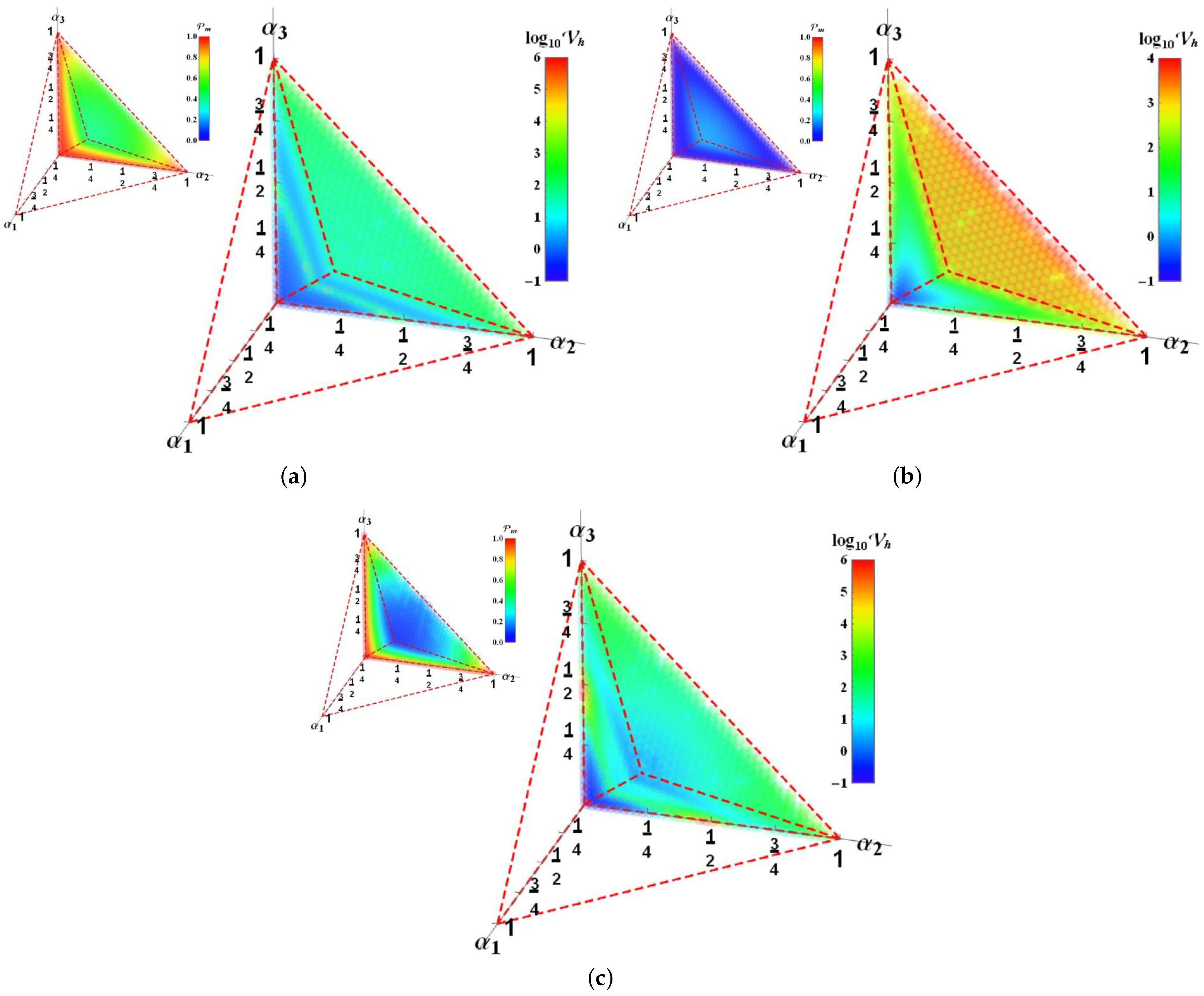
By following the procedure previously depicted, we were able to get the minimum of QFI on the Bloch sphere for a sample of at least ${10}^4$ points on the parametric space. Such a procedure was programmed and run on a $1.9$ GHz processor using a $4$—core parallel processing. The entire procedure last out a couple of hours for sequential channels. A doubly detailed calculation clearly rises the time processing by a factor of eight. The output has been represented on Figure 7 for (a) $n=1$, (b) $n=2$, (c) $n=3$, and (d) $n=4$. Each calculation on each point of the parametric space was then represented with a coloured point of finite size (to produce a continuous variation of the values on the region) using a log scale for ${\mathcal{V}}_h$ in colour. The equivalence for the colour scale is represented in the colour bar besides on the right. Unfortunately, the outcomes scales are dramatically different to set a common colour scale for the four cases, then a particular scale is used in each case.

Noting QFI and ${\mathcal{V}}_h$ are symmetric under a cyclic exchange of ${\alpha }_1,{\alpha }_2,{\alpha }_3$ because $f_i$ for the sequential channels and $f_i^{\mathrm{ICO}}$ for the ICO channels are also cyclic. In fact, Formulas (32) and (33) and the procedure depicted before and comprised in (36), depict such a symmetry. Then, to depict the inner region of the parametric space, we only represent a third part of it. In some regions, ${\mathcal{V}}_h$ changes fast appearing be discontinuous due to the finite size of the mesh. Despite, calculation is completely precise on each selected point, but represented by a point of finite size.

Although sequential cases with an increasing n commonly give larger values for ${\mathcal{V}}_h$ in the entire parametric region, they also include some particular regions with lower values, the four characteristic syndrome channels: transparent, BFN, DN, and their combination. For $n>1$, we realize that regions near to $2({\alpha }_i+{\alpha }_j)=1,i\ne j\in \{1,2,3\}$ give the largest values for ${\mathcal{V}}_{\mathrm{h}}$ and sometimes with $\mathcal{F}$ singular (reddest regions). Those three possible regions meet on the depolarizing channel located in the center of the entire parametric space. Then, as it was expected, those are the channels with the worst estimation parameter by using such procedures based on a sequential application strategy. We set a proper comparison after presenting the corresponding outcomes for ICO arrangements in the next section.

5.1.2. Multi-Parametric Estimation: ICO Channels Case

The same procedure is followed for ICO arrangements of Pauli channels. Due to the higher complexity to set the form factors given in Formulas (32)–(36), the calculation procedure produces larger formulas as those reported in the Appendix B. It gives rising processing times around 12 h or more to sweep the entire parametric region finding the minimum values for ${\mathcal{V}}_h$. Outcomes are represented in Figure 8 by following the same methodology and representation than those of sequential arrangements. Together, as an upper-left inset, the values for ${\mathcal{P}}_m$ are represented there. Remembering that the ICO procedure being presented is in fact a stochastically one, such inset is useful to catch the real utility of each parameter procedure.

For instance, ICO arrangement for $n=3$ becomes few useful because the lower values of ${\mathcal{P}}_m$ in the most channels cases. Such aspect was already noticed in [11]. A new aspect is observed by noticing despite the channels on the frontal face, ${\alpha }_0=0$, exhibits perfect unitary fidelities thus behaving as transparent ones, it has not always behaved well for QPE purposes (despite ICO schemes become almost optimal for the nearest channels to the transparent one). Despite this, certain channels under ICO exhibit a better behaviour for QPE as it will be seen in the next section by characterizing each type of scheme.

5.2. Characterizing the Best Parametric Estimation and Value of ICO Schemes

In this case, the affordable regions to get an advantaged procedure over other ones are centered on the transparent and central ICO channels. Note the clear differences between the even and odd cases reported. Those differences already were noticed for the single QPE on Figure 6, highlighting the role of ICO case with $n=2$.

Table 1. Variability ranges reached for certain optimal test states for the minimum of ${log}_{10}{{\mathcal{V}}_h}_n^{Seq}$ and ${log}_{10}{{\mathcal{V}}_h}_n^{\pm ICO}$ for Pauli channels on the entire parametric space. First column for sequential channels, and second one for stochastic channels under ICO.

n	${{\mathcal{V}}_{\mathit{h}}}_{\mathit{n}}^{\mathit{Seq}}$	${{\mathcal{V}}_{\mathit{h}}}_{\mathit{n}}^{\pm \mathit{ICO}}$
	$[{\mathbf{log}}_{\mathbf{10}}{{\mathcal{V}}_{\mathit{h}}}_{{\mathit{n}}_{\mathbf{min}}}^{\mathit{Seq}},{\mathbf{log}}_{\mathbf{10}}{{\mathcal{V}}_{\mathit{h}}}_{{\mathit{n}}_{\mathbf{max}}}^{\mathit{Seq}}$]	$[{\mathbf{log}}_{\mathbf{10}}{{\mathcal{V}}_{\mathit{h}}}_{{\mathit{n}}_{\mathbf{min}}}^{\mathbf{\pm }\mathit{ICO}},{\mathbf{log}}_{\mathbf{10}}{{\mathcal{V}}_{\mathit{h}}}_{{\mathit{n}}_{\mathbf{max}}}^{\pm \mathit{ICO}}$]
1	$[+0.0289,+0.2287]$	−
2	$[-0.5003,+3.3758]$	$[-0.3914,+5.4543]$
3	$[-0.7830,+6.9481]$	$[-0.7620,+3.9795]$
4	$[-0.9665,+10.678]$	$[-0.9346,+6.5031]$

summarizes the variability ranges for $log{\mathcal{V}}_h$ obtained numerically with the procedure previously depicted for each method analysed. Second column includes the sequential arrangements, and the third, the ICO ones. Note the dramatic increasing in the upper limit by using larger sequential arrangements despite the little gaining on the lower limit. Note particularly than the upper limit is only representative of the numerical calculation performed because in fact for $n=2,3,4$, $log{\mathcal{V}}_h\to \infty$ in the places where $\mathcal{F}$ becomes singular.

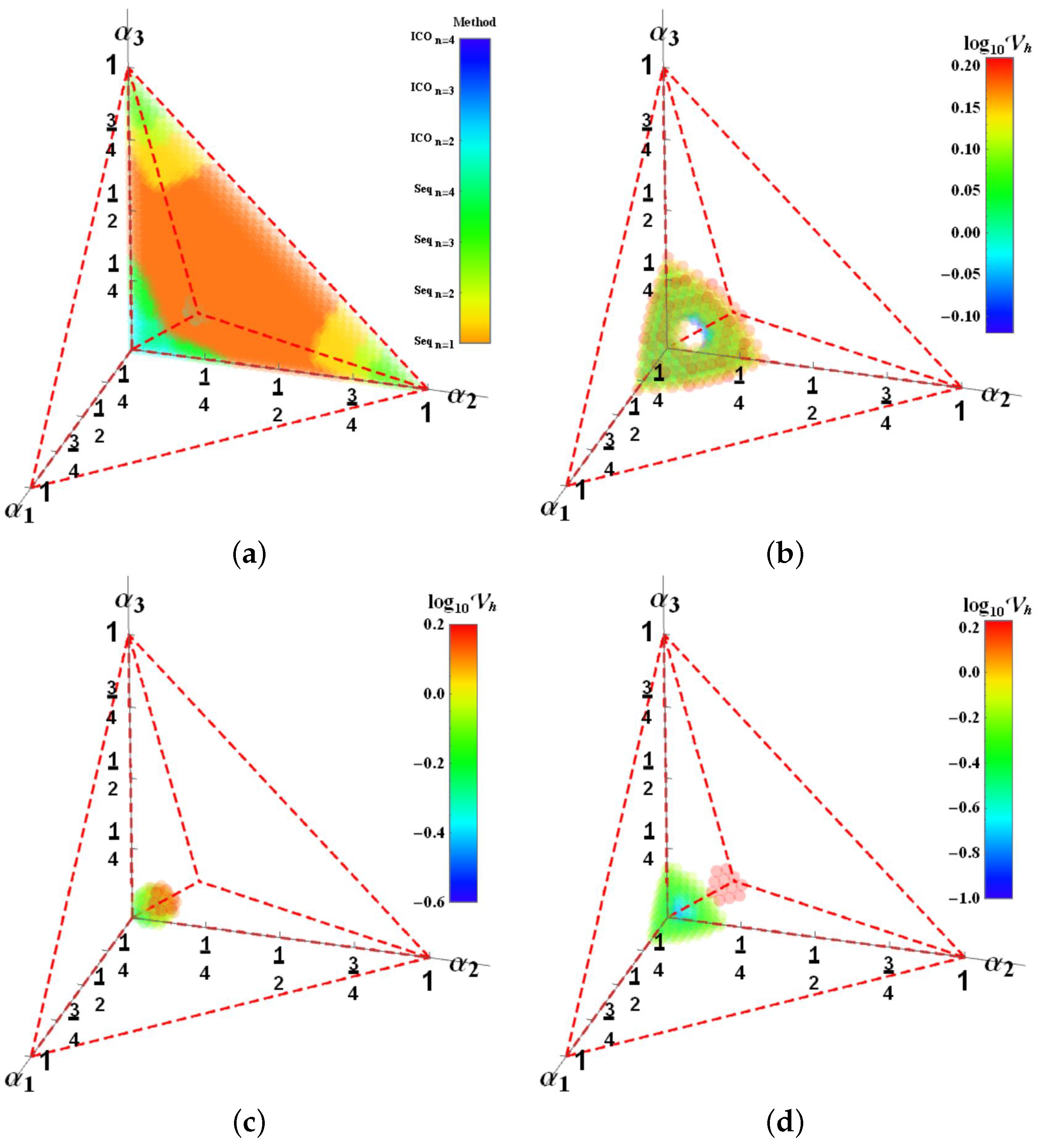
Despite the ranges on Table 1, advantages for the ICO arrangements could occur because the lowest limits reported there (as instance for sequential channels with $n\ge 1$) correspond only to specific channels with the best scenario for the overall cases. In a big picture view, Figure 9a shows the channel parametric region gathering the best method for each channel depicted in colour in agreement with the legend on the right. Note the direct single Pauli channels dominates the most of them. Despite this, channels around of BFN, DN, and their combination will become better analysed for QPE purposes with sequential arrangements. The ICO arrangements for $n=2,3,4$ becomes particularly useful for different zones near to the transparent Pauli channel, but notably, channels near to the central ICO channel becomes better analysed with the ICO arrangement using $n=4$ Pauli channels.

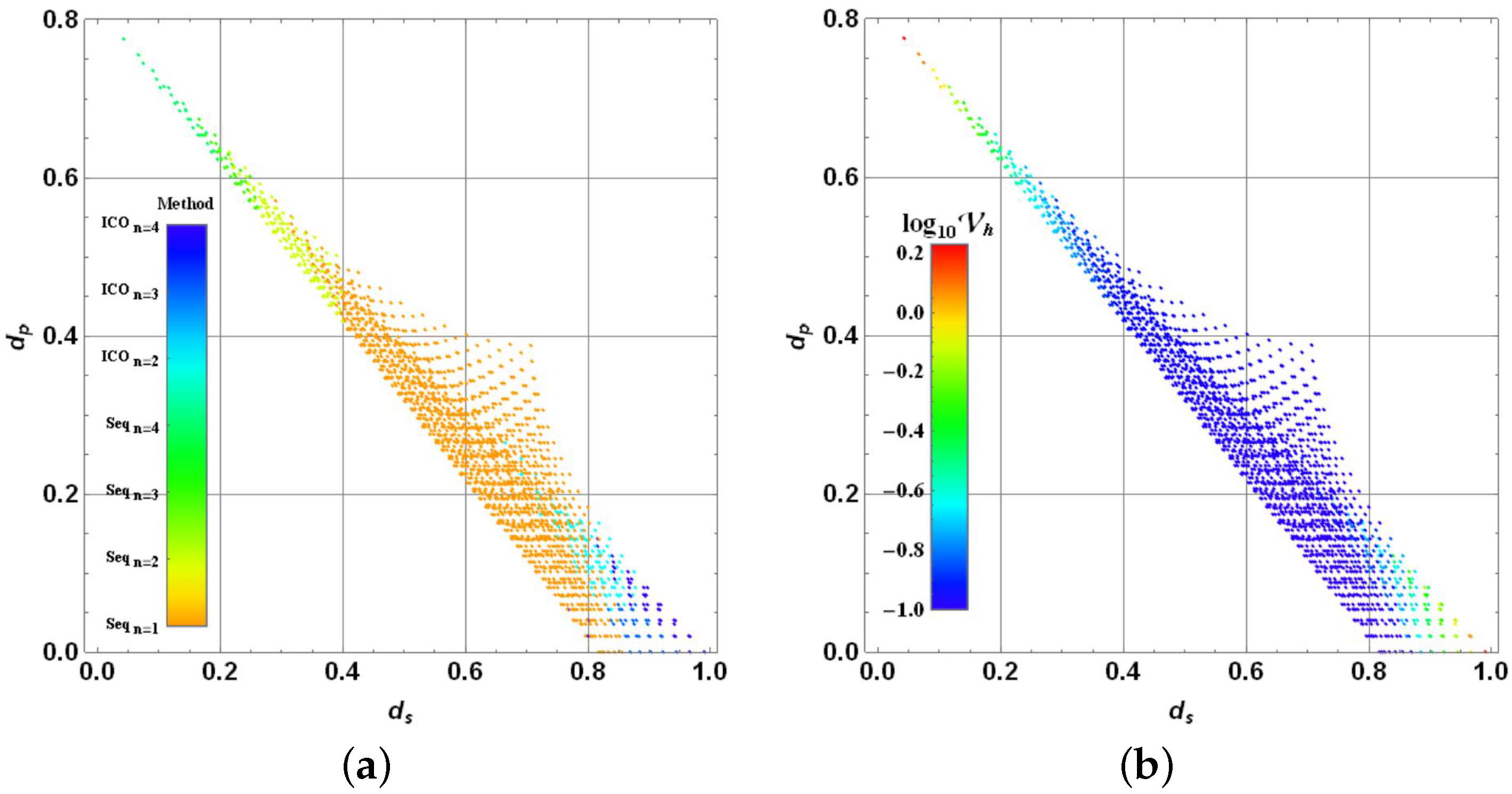
Figure 9b–d include only the corresponding points to each region where ICO arrangements will give better values for QPE (with $n=2,3,4$, respectively). In each plot, colour still reports the values of ${log}_{10}{{\mathcal{V}}_h}_{n_{\min }}^{\pm ICO}$ in agreement with the colour scale in the colour bar being included. In any case, values for ${{\mathcal{V}}_h}_{n_{\min }}$ do not surpass ${10}^{0.2}$. A notable pattern should be noticed. Although a single channel strategy gives better outcomes in the central body of the region, sequential arrangements of identical channels deliver better results for QPE in the corners where just one of the ${\alpha }_i$ parameters rules the channel (near to the syndrome channels, such as BFN, DN, or their combination). Finally, ICO stochastic arrangements shows their efficiency in the central region where ${\alpha }_1\approx {\alpha }_2\approx {\alpha }_3$, precisely like our initial previous analysis with the single parameter p. Figure 10a,b shows such an analysis. By defining $d_s$ for each Pauli channel in the parametric space as the minimum distance to any of the syndrome corners and $d_p$ as the minimum distance to the central line where ${\alpha }_1={\alpha }_2={\alpha }_3$. Then, Figure 10a reproduces the classification for each best method presented in Figure 9a. Each point represents to each one of the more than ${10}^4$ channels analysed through of the entire parametric region. The efficiency of each procedure is seen to fulfill the mentioned criteria. Figure 10b reports the same arrangement but in this case the colour shows the ${log}_{10}{\mathcal{V}}_h$ value in agreement with the colour bar beside. Findings on the last plot agree with the previous ones. Thus, blue region corresponds to the single channel arrangement, where such strategy gives the lower CRB. The reddest points correspond to those closer to the central ICO channel ($d_s\approx 0,d_p\approx \sqrt{2/3}\approx 0.8$), while, greenest corresponds to those near to the syndromes BFN, DN, and their combination, where sequential strategy gives the better outcome for the QPE.

The latest compared outcomes show that despite ICO arrangements of Pauli channels are able to exhibit an induced transparency [11], while sequential arrangements commonly induces opacity, still it has not parallel outcomes for QPE. Combined strategies should be considered to sweep effectively the entire Pauli channels region for parameter estimation purposes. Such behaviour has been already noticed in previous works regarding ICO approaches for single parameter channels [28,30].

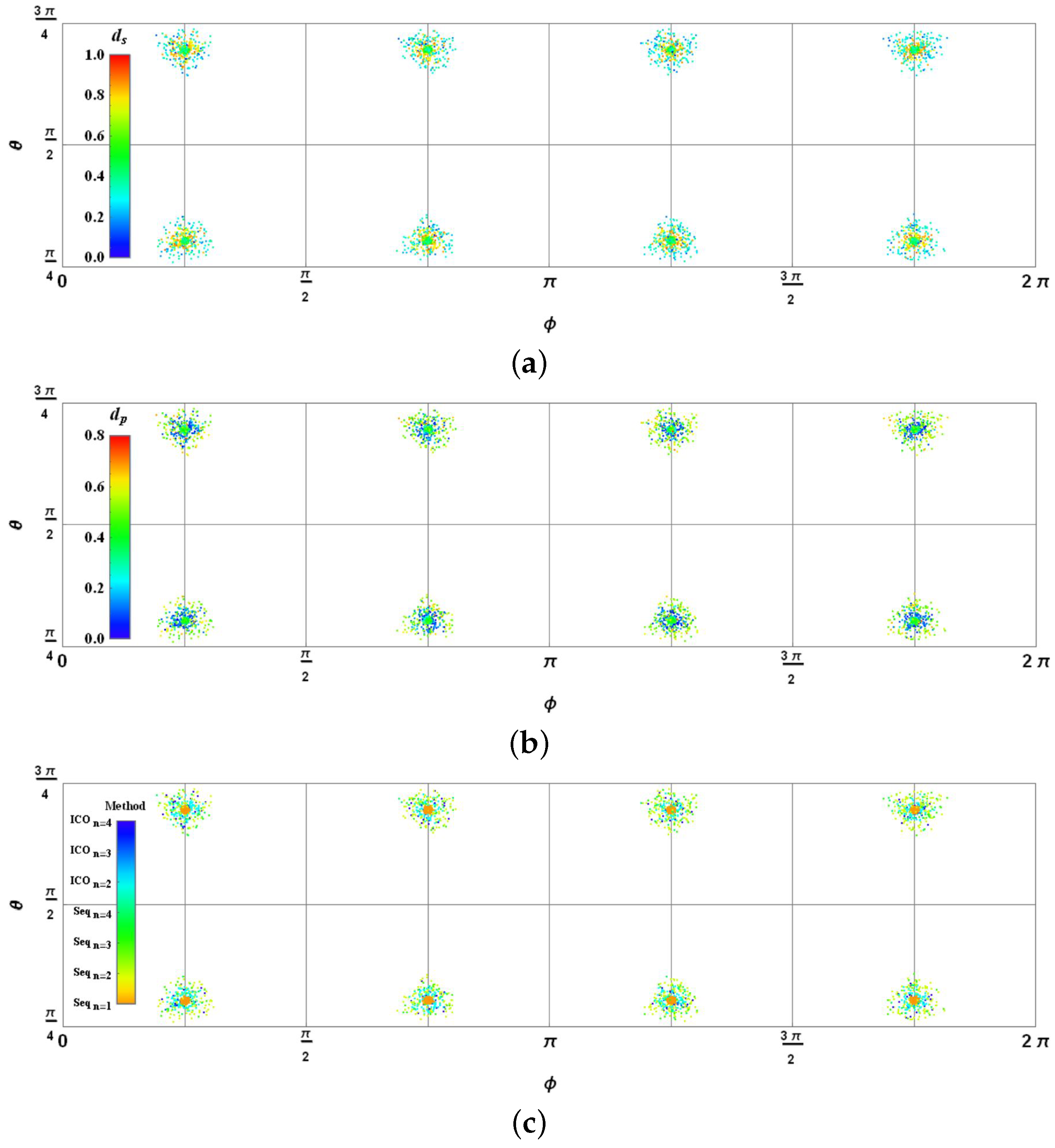
Finally, we explore the optimal test states to reach the best outcome for QPE with a proper method or arrangement. Plots in Figure 11 comprise the test states for the best strategy found. All points are represented on a flat representation of the Bloch sphere $\theta \in [0,\pi ],\varphi \in [0,2\pi ]$, with $\theta$ scale reduced to represent just the meaningful region. In each one, points are the same, but colouring represents (a) $d_s$, (b) $d_p$, and (c) the best method or arrangement, in agreement with the corresponding colour scale included. Interestingly, they are concentrated on little accumulation clusters. In Figure 11c, on each cluster, the central region corresponds to those channels with a middle distance $d_s$ and $d_p$. It means that, where the single channel strategy, the reddest points are the best. Around where other arrangements are located, the bluest are for those using ICO arrangements and the greenest are for those using sequential ones. Information on Figure 11a,b is similar and consistent with the previous in agreement with the definitions of $d_s$ and $d_p$.

6. Conclusions

Improvements to QPE have been pursued as a hot topic in quantum information in recent decades. The importance of quantum channels in quantum communication is in the core of applications related with quantum memories [38], quantum processing, and many other applications exploiting the transmission or processing of information. Therefore, the use of QFI has become essential to bound the parametric design and identification of those quantum channels [2]. By considering thoughtful alternative arrangements of well-identified single quantum channels, it has been expected to improve their parametric characterization bounding. In fact, by considering more thoughtful arrangements in superposition [39,40], some not only considering the related channels subject to estimation instead of additional configurable elements, some improvements have been recently introduced for the single parameter quantum switch (it means around the depolarizing channel). Those arrangements include sequential, parallel, ICO, and path superposition methods [41,42]. Each one contributing with improvements in different regions for the values of the involved parameter.

Still sequential arrangements of Pauli channels are expected to imprint redundant traits of the channels to then being identified with a relative higher precision in agreement with the Cramér–Rao bound. However, it is a fact that, with the development of indefinite causal structures, a new route or research for QPE has been suggested and partially proved in this terrain [28,30]. Therefore, quantum switch was the first channel to be characterized under this approach due to its dramatic properties when it is quantumly modified under the control of a causal structure [5]. For such a reason, the depolarizing channel has been widely studied in QPE [28,41]. Despite this, QPE should be open for arbitrary channels using similar causal structures. Thus, for qubits, together with Pauli channels, the parametric estimation has an important research arena due to its well-known algebraic properties [11].

In this way, in the current development, we are extending the analysis for an entire family of channels widely implemented in quantum processing, Pauli channels. Such a set of channels are clearly parameterized by a triplet of numbers generating their quantum communication properties. Then, the use of causal structures compared with alternative sequential arrangements has shown each scheme reduces in a different strength the effective bound for QPE. As shown in [11], despite ICO is not a generic solution to improve quantum communication, still it has demonstrated to improve in great extent certain process in that terrain [34,35].

For the current analysis, we have characterized the parametric space of Pauli channels in terms of the bound for multi-parametric QPE by comparatively using sequential and ICO arrangements. The use of single channels works reasonably at certain strength for parametric estimation regarding channels evenly mixing the three pure communication syndromes (bit-flipping, dephasing, and their combination). Instead, for channels exhibiting an almost pure communication syndrome, then the sequential strategy notably reduces the QPE bounds in comparison with the single channel strategy. Thus, sequential arrangements show advantages for QPE near of dephasing and bit-flipping noise channels (or their combination). Finally, some channels susceptible to exhibit transparency (natural or induced by an ICO scheme [11]) are notably better analysed precisely with an ICO arrangement strategy. Notably, ICO schemes with a larger n work better near from the central ICO channel (the channel exhibiting perfect transparency for the most imperfect teleportation channel [34]).

On the road, we have extended the analysis for Pauli channels arrangements under an ICO schemes by getting an analytic procedure to reach expressions for the corresponding output state ${\Lambda }_m^n\left[\rho \right]$. It extends the analysis introduced in [11] for those arrangements developed for channels with ${\alpha }_0=0$ in the frontal face of the parametric space. Despite our development to analyse QPE with ICO arrangements, such procedure is not limited to the post-measurement case. It could be useful to get analytic expressions for ${\Lambda }^n[\rho \otimes {\rho }_C]$ and particularly for the factor forms $f_n^{\mathrm{ICO}}$ in alternative ICO schemes.

In [31], for qudits, notable values for the CRB were found for the depolarizing channel under ICO in a considerable region of the channel parameter (a channel with a different construction than here in terms of its parameter). Here, sequential channels give higher bounds around the depolarizing channel than the single channel strategy (when the parameter is responsible to sweep the Pauli channels family). As it is well-known, ICO arrangements circumvent the opacity problem for such a channel generating partial transparency thus reducing the parameter information carried out.

In this work, for qubits, we are swept the entire Pauli channels family comparing single, sequential, and ICO arrangements for multi-parametric QPE, obtaining still a reduced range for such a bound by choosing the best method for each channel. Thus, our best outcomes ranges for ${\mathcal{V}}_h$ between ${10}^{-1}$ and ${10}^{0.2}$ when ICO is used (see Figure 9). Some of those values are still large for the estimation variance of parameter values around one. There are other limitations, such as for the ICO arrangement with $n=3,4$ are the low success probabilities for some of those channels under the stochastic method being considered.

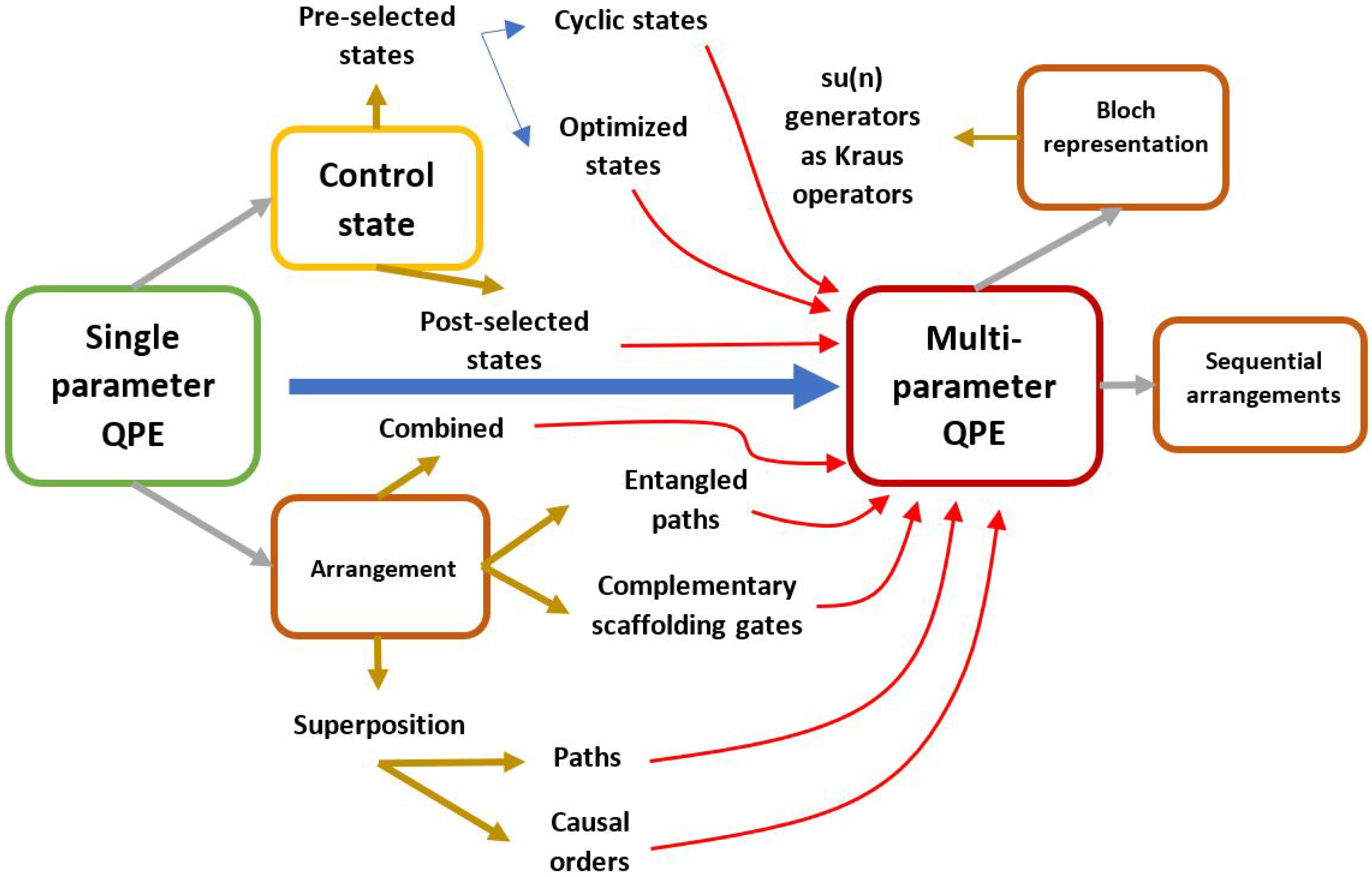
Future work in the QPE trend followed in the current work (multi-parametric QPE analysis for Pauli channels) should consider alternative superposition arrangements (paths or causal orders). Some proposals have been recently presented for the single parameter case by including complementary elements in the form of unitary gates boosting the estimation [42]. Additionally, ICO arrangements should be considered under other alternative procedures than the stochastic one. It will mean without control state post-selection as in [28]. Then, it will involve the task to optimize the initial state for the control system or to probe certain well-known initial control states as the cyclic control states [10]. Alternative trends have suggested the use of entangled arrangements [31]. Despite this, optimization over an extended group of parameters appears unavoidable (on probe states, control states, and complementary parameters in the setup). Note that the development obtained in Section 3 is still useful for such a task. Another interesting extension is to consider qudits under a similar approach. By using Bloch representation for qudits, similar formulas to express QFI as (11) are known [26]. Equivalent channels to Pauli ones are could be considered in terms of the $su\left(n\right),n>2$ algebra generators. Despite being more complex (due to the structure constants), it could still contribute to analysis, in a similar way, of the corresponding output state for an associated ICO arrangement. A summarized roadmap of possible future work in a similar trend to the current development is shown in Figure 12. Those possible extensions for the current development in the remarked directions surely will contribute to dramatically reduce the CRB in QPE for different types of quantum channels. Such a reduction will encourage the development of concrete methods to analyse quantum channels reaching their parametric characterization still for the multi-parametric case.

Such optimal methods still should be followed with the construction of adequate observables in each case. They should be measured on the arrangements and proper probe states found in the QPE analysis. The affordability of each construction for practical quantum metrology will be supported by the theoretical CRB being pursued with concrete measurement techniques as it was illustrated on Figure 4. Alternative more complex techniques still could provide sharper bounds exploring Holevo information [43,44], which, for ICO arrangements is still in the same direction of analysis commonly followed [8]. Still, such a construction could not be trivial due to the incompatibility among different physical quantities used as observables (when conjugate variables are precised). It states a limit on the attainable precision together with the dependence of the arrangement method on the concrete parameter values to be estimated [45,46]. Despite these obstacles, some experimental approaches have been already developed in quantum phase and phase diffusion estimation [47,48]. In fact, further than the limitations imposed by the CRB, still there are lots of challenges in quantum metrology to get a proper characterization of unknown quantum channels through measurements. Despite this, theoretical and experimental work is intensely being developed to supersede some of those obstacles.

References

- Fisher, R.A. On the Mathematical Foundations of Theoretical Statistics. Philos. Trans. R. Soc. Lond. A 1922, 222, 309–368. [Google Scholar]
- Helstrom, C. Quantum Detection and Estimation Theory; Academic Press: New York, NY, USA, 1976. [Google Scholar]
- Frey, M.; Coffey, L.; Mentch, L.; Miller, A.; Rubin, S. Correlation Identification In Bipartite Pauli Channels. Int. J. Quantum Inf. 2010, 8, 979–990. [Google Scholar] [CrossRef]
- Chiribella, G.; D’Ariano, G.M.; Perinotti, P.; Valiron, B. Quantum computations without definite causal structure. Phys. Rev. A 2013, 88, 022318. [Google Scholar] [CrossRef]
- Ebler, D.; Salek, S.; Chiribella, G. Enhanced Communication With the Assistance of Indefinite Causal Order. Phys. Rev. Lett. 2017, 120, 120502. [Google Scholar] [CrossRef]
- Goswami, K.; Cao, Y.; Paz-Silva, G.A.; Romero, J.; White, A. Communicating via ignorance. Phys. Rev. Res. 2018, 2, 033292. [Google Scholar] [CrossRef]
- Procopio, L.M.; Moqanaki, A.; Araujo, M.; Costa, F.; Calafell, I.A.; Dowd, E.G.; Hamel, D.R.; Rozema, L.A.; Brukner, C.; Walther, P. Experimental superposition of orders of quantum gates. Nat. Commun. 2015, 6, 7913. [Google Scholar] [CrossRef]
- Procopio, L.M.; Delgado, F.; Enríquez, M.; Belabas, N.; Levenson, J.A. Communication enhancement through quantum coherent control of N channels in an indefinite causal-order scenario. Entropy 2019, 21, 1012. [Google Scholar] [CrossRef]
- Procopio, L.M.; Delgado, F.; Enríquez, M.; Belabas, N.; Levenson, J.A. Sending classical information via three noisy channels in superposition of causal orders. Phys. Rev. A 2020, 101, 012346. [Google Scholar] [CrossRef]
- Chiribella, G.; Wilson, M.; Chau, H.F. Quantum and Classical Data Transmission through Completely Depolarizing Channels in a Superposition of Cyclic Orders. Phys. Rev. Lett. 2021, 127, 190502. [Google Scholar] [CrossRef]
- Delgado, F.; Cardoso-Isidoro, C. Performance characterization of Pauli channels assisted by indefinite causal order and post-measurement. Quantum Inf. Comput. 2020, 20, 1261–1280. [Google Scholar] [CrossRef]
- Lehmann, E.L.; Casella, G. Theory of Point Estimation; Springer: New York, NY, USA, 1986. [Google Scholar]
- Rao, C.R. Information and accuracy attainable in the estimation of statistical parameters. Bull. Calcutta Math. Soc. Springer Ser. Stat. 1945, 37, 81–91. [Google Scholar]
- Liu, J.; Yuan, H.; Lu, X.; Wang, X. Quantum Fisher information matrix and multiparameter estimation. J. Phys. A Math. Theor. 2020, 53, 023001. [Google Scholar] [CrossRef]
- Šafránek, D. Simple expression for the quantum Fisher information matrix. Phys. Rev. A 2018, 97, 042322. [Google Scholar] [CrossRef]
- Frieden, B.R.; Gatenby, R.A. Principle of maximum Fisher information from Hardy’s axioms applied to statistical systems. Phys. Rev. E 2013, 88, 042144. [Google Scholar] [CrossRef] [PubMed]
- Kraus, K. States, Effects and Operations: Fundamental Notions of Quantum Theory; Springer: Berlin, Germany, 1983. [Google Scholar]
- Ritter, W.G. Quantum channels and representation theory. J. Math. Phys. 2005, 46, 082103. [Google Scholar] [CrossRef]
- Petz, D. Quantum Information Theory and Quantum Statistics; Springer: Berlin, Germany, 2008. [Google Scholar]
- Flammia, S.T.; Wallman, J.J. Efficient estimation of Pauli channels. arXiv 2019, arXiv:1907.12976. [Google Scholar] [CrossRef]
- Nielsen, M.A.; Chuang, I.L. Quantum Computation and Quantum Information, 10th Anniversary ed.; Cambridge University Press: Cambridge, UK, 2000. [Google Scholar]
- Katarzyna, S. Geometry of Pauli maps and Pauli channels. Phys. Rev. A 2019, 100, 062331. [Google Scholar]
- Fujiwara, A.; Imai, H. Quantum parameter estimation of a generalized Pauli channel. J. Phys. A Math. Gen. 2003, 36, 8093. [Google Scholar] [CrossRef]
- Rehman, J.; Shin, H. Entanglement-Free Parameter Estimation of Generalized Pauli Channels. Quantum 2021, 5, 490. [Google Scholar] [CrossRef]
- Dittmann, J. Explicit formulae for the Bures metric. J. Phys. A Math. Gen. 1999, 32, 2663. [Google Scholar] [CrossRef]
- Zhong, W.; Sun, Z.; Ma, J.; Wang, X.; Nori, F. Fisher information under decoherence in Bloch representation. Phys. Rev. A 2011, 87, 022337. [Google Scholar] [CrossRef]
- Blondeau, F. Quantum parameter estimation on coherently superposed noisy channels. Phys. Rev. A 2021, 104, 032214. [Google Scholar] [CrossRef]
- Frey, M. Indefinite causal order aids quantum depolarizing channel identification. Quantum Inf. Process. 2019, 18, 96. [Google Scholar] [CrossRef]
- Blondeau, F. Noisy quantum metrology with the assistance of indefinite causal order. Phys. Rev. A 2021, 103, 032615. [Google Scholar] [CrossRef]
- Frey, M.; Collins, D. Quantum Fisher information and the qudit depolarization channel. In Proceedings of the SPIE 7342, Quantum Information and Computation VII, Orlando, FL, USA, 27 April 2009; p. 73420N. [Google Scholar]
- Frey, M.; Collins, D.; Gerlach, K. Probing the qudit depolarizing channel. J. Phys. A Math. Theor. 2011, 44, 205306. [Google Scholar] [CrossRef]
- Fujiwara, A. Quantum channel identification problem. Phys. Rev. A 2001, 63, 042304. [Google Scholar] [CrossRef]
- Arvidsson-Shukur, D.; Halpern, N.; Lepage, H.; Lasek, A.; Barnes, C.; Lloyd, S. Quantum advantage in postselected metrology. Nat. Commun. 2020, 11, 3775. [Google Scholar] [CrossRef] [PubMed]
- Cardoso-Isidoro, C.; Delgado, F. Symmetries in Teleportation Assisted by N-Channels under Indefinite Causal Order and Post-Measurement. Entropy 2020, 12, 1904. [Google Scholar] [CrossRef]
- Mukhopadhyay, C.; Pati, A. Superposition of causal order enables quantum advantage in teleportation under very noisy channels. J. Phys. Commun. 2020, 4, 105003. [Google Scholar] [CrossRef]
- Seveso, L.; Albarelli, F.; Genoni, M.G.; Paris, M.G.A. On the discontinuity of the quantum Fisher information for quantum statistical models with parameter dependent rank. J. Phys. A Math. Theor. 2019, 53, 02LT01. [Google Scholar] [CrossRef]
- Šafránek, D. Discontinuities of the quantum Fisher information and the Bures metric. Phys. Rev. A 2017, 95, 052320. [Google Scholar] [CrossRef]
- Le Gouët, J.L.; Moiseev, S. Quantum Memory. J. Phys. B At. Mol. Opt. Phys. 2012, 45, 120201. [Google Scholar] [CrossRef]
- Chiribella, G. Perfect discrimination of nosignalling channels via quantum superposition of causal structures. Phys. Rev. A 2012, 86, 040301. [Google Scholar] [CrossRef] [Green Version]
- Abbott, A.; Wechs, J.; Horsman, D.; Mhalla, M.; Branciard, C. Communication through coherent control of quantum channels. Quantum 2020, 4, 333. [Google Scholar] [CrossRef]
- Procopio, L. Parameter estimation via indefinite causal structures. arXiv 2022, arXiv:2207.04838. [Google Scholar]
- Liu, Q.; Hu, Z.; Yuan, H.; Yang, Y. Strict Hierarchy of Strategies for Non-asymptotic Quantum Metrology. arXiv 2022, arXiv:2203.09758. [Google Scholar]
- Demkowicz-Dobrza, R.; Górecki, W. Multi-parameter estimation beyond quantum Fisher information. J. Phys. A Math. Theor. 2020, 53, 363001. [Google Scholar] [CrossRef]
- Yang, Y.; Shihao, R.; An, M.; Wang, Y.; Wang, F.; Zhang, P.; Li, F. Multiparameter simultaneous optimal estimation with an SU(2) coding unitary evolution. Phys. Rev. A 2022, 105, 022406. [Google Scholar] [CrossRef]
- Miyazaki, J.; Matsumoto, K. Imaginarity-free quantum multiparameter estimation. Quantum 2022, 6, 665. [Google Scholar] [CrossRef]
- Len, Y.L. Multiparameter estimation for qubit states with collective measurements: A case study. New J. Phys. 2022, 24, 033037. [Google Scholar] [CrossRef]
- Szczykulska, M.; Baumgratz, T.; Datta, A. Reaching for the quantum limits in the simultaneous estimation of phase and phase diffusion. Quantum Sci. Technol. 2017, 2, 044004. [Google Scholar] [CrossRef]
- Roccia, E.; Cimini, V.; Sbroscia, M.; Gianani, I.; Ruggiero, L.; Mancino, L.; Genoni, M.; Ricci, M.A.; Barbieri, M. Multiparameter approach to quantum phase estimation with limited visibility. Optica 2018, 5, 1171–1176. [Google Scholar] [CrossRef] [Green Version]
Figure 1.
Process for QPE of a quantum channel. A well-defined input quantum resource is sent through the channel emerging and carrying out information about it in the output state. It is measured on a selected basis corresponding to certain observable to then infer the nature of the parameter channel.
Figure 2.
(a) Single channel characterization in the parametric space remarking some emblematic channels, and (b) sequential identical channels arrangements.
Figure 3.
Communication channels arranged in a definite causal order as function of the control states . They become in indefinite causal order by considering a superposition of them.
Figure 4.
Process for QPE of a controlled quantum channel as in ICO case. An intermediate measurement on the control system is performed, if it is successful obtaining the adequate control state, the QPE process continues.
Figure 5.
QFI for Pauli sequential channels, , with a single parameter for (a) Mixed states, and (b) Pure states. Each line depicts the behaviour of for each value of n. Gray planes remarks the zone where the totally depolarizing channel is, .
Figure 6.
QFI for Pauli ICO channels, , with a single parameter for (a) Mixed states and (b) Pure states. Each line depicts the behaviour of for each value of n considered. Gray planes remarks the zone where the totally depolarizing channel is, . (c) The probability of success distribution in the stochastic measurement on the control state.
Figure 7.
In colour, lowest for certain optimal test state using Pauli channels under a sequential application considering mixed output states for (a) , (b) , (c) , and (d) . Representation is constructed on the entire channel parametric space . Scale is reported in agreement with the colour bar beside.
Figure 8.
In colour, lowest for certain optimal test state using Pauli channels under ICO application considering mixed output states for (a) , (b) , and (c) . Representation is constructed on the entire channel parametric space . Scale is reported in agreement with the colour bar beside. Upper-left inset shows in colour for the stochastic process with its respective colour bar scale.
Figure 9.
(a) Best possible method for multi-parametric estimation indicated in the colour scale for the entire parametric region. (b) , (c) , and (d) regions where ICO with those number of channels combined become advantaged with respect the remaining methods analysed. Colour reports the corresponding value in agreement with the bar beside.
Figure 10.
(a) Best possible method for multi-parametric estimation indicated in the colour scale for the entire parametric region as function of and . (b) Same arrangement for the previous plot but showing in colour the best value in agreement with the left bar.
Figure 11.
Corresponding optimal test states for each Pauli channel under the properly method or arrangement reported in Figure 9 and Figure 10. Colouring corresponds to (a) , (b) , and (c) the best method or arrangement, in agreement with each colour bar.
Figure 12.
Some viable variations to develop QPE for the multi-parametric channels by following the trends developed in the current research. Some novel developments in single parameter QPE could be directly applied to the multi-parametric case.