Dynamic Behavior of a Fractional-Type Fuzzy Difference System

Abstract

In this paper, our aim is to study the following fuzzy system: $x_{n+1}=\frac{A{x}_{n-1}{x}_{n-2}+B{x}_{n-3}}{D+C{x}_{n-4}},n=0,1,2,\cdots ,$ where $\{x_n\}$ is a sequence of positive fuzzy numbers and the initial conditions $x_{-4},x_{-3},x_{-2},x_{-1},x_0$ and the parameters $A,B,C,D$ are positive fuzzy numbers. Firstly, the existence and uniqueness of positive fuzzy solutions of the fuzzy system are proved. Secondly, the dynamic behavior of the equilibrium points for the fuzzy system are studied by means of the fuzzy sets theory, linearization method and mathematical induction. Finally, the results obtained in this paper are simulated by using the software package MATLAB 2016, and the numerical results not only show the dynamic behavior of the solutions for the fuzzy system, but also verify the effectiveness of the proposed results.

1. Introduction

Just as differential equations are called continuous dynamical systems, difference equations are called discrete dynamical systems that play a very important role in describing many problems in the real world. For example, when describing continuous variables such as parameter $t$, where $t\in T$, mathematical models for many practical problems can be established by differential equations (see, e.g., [1,2,3,4,5,6,7,8,9,10,11] and the references therein). However, many variables in the real world are not necessarily continuous in performance—we call them discrete variables—such as number of times, days, and so on. Therefore, the use of difference equations can better reflect and solve practical problems in the establishment of such mathematical models (see, e.g., [12,13,14,15,16] and the references therein). With the development and popularization of computer technology, the applications of difference equation models are more and more extensive. For example, they have been applied in biology, ecology, biomedical engineering, economics, finance, demography, automatic control theory, information communication theory, computer network, and other fields (see, e.g., [17,18,19,20,21]). Because difference equations are dynamic systems with discrete variables, they are easier to calculate and simulate with computers than differential equations are. Moreover, for some differential equations, the continuous variables are sometimes discretized and transformed into the corresponding difference equations, which can be used for numerical calculation and simulation on computers (see, e.g., [22,23,24,25,26,27,28,29,30,31,32,33] and the references therein). This has stimulated scholars’ enthusiasm for the study of difference equations and promoted the development of difference equations. However, since the data and information of difference systems describing many practical problems are uncertain, and fuzzy set theory is a very powerful tool for processing fuzzy information in mathematical models, it is very interesting to study the dynamic behavior of the solution of a fuzzy difference system, where the initial value and parameters are fuzzy numbers and the solution is a sequence of fuzzy numbers (see, e.g., [34,35,36,37,38,39]). Compared with classical difference systems, fuzzy difference systems can more accurately describe actual problems, so the study of fuzzy difference systems has become an important part of difference system theory.

As an important mathematical model describing the natural phenomena and objective laws in the real world, difference systems have attracted many scholars’ attention, and their theory has been rapidly developed since the 1990s. In the existing research results on difference equations, a typical monograph includes V. L. Kocic and G. Ladas’s works [40] published in 1993. The monograph became the guidance book for later researchers. In particular, the professional journals of international difference equation studies, named separately “Journal of Difference Equations and Applications”, founded in 1995, and “Advances in Difference Equations”, founded in 2004, have further promoted the study of difference equation theory. What must be pointed out is that M.R.S. Kulenovic and G. Ladas [41] discussed the properties of solutions for the following second-order difference equation:

$$x_{n+1}=\frac{\alpha +\beta x_n+\delta x_{n-1}}{A+B{x}_n+C{x}_{n-1}},n=1,2,\cdots ,$$

(1)

where the parameters $\alpha ,\beta ,\delta ,A,B,C$ and the initial conditions $x_0,x_1$ are positive real numbers. In 2007, E. Camouzis and G. Ladas [42] studied the properties of solutions for the third-order difference equation

$$x_{n+1}=\frac{\alpha +\beta x_n+\gamma x_{n-1}+\delta x_{n-2}}{A+B{x}_n+C{x}_{n-1}+D{x}_{n-2}},n=1,2,\cdots ,$$

(2)

where the parameters $\alpha ,\beta ,\gamma ,\delta ,A,B,C,D$ and the initial conditions $x_{-1},x_0,x_1$ are positive real numbers. In addition, we should mention that in 1996, Deeba et al. [43] studied the first order fuzzy difference equation

$$x_{n+1}=w{x}_n+q,n=0,1,\cdots ,$$

(3)

where $\{x_n\}$ is a sequence of fuzzy numbers and $x_0,q,w$ are fuzzy numbers, which arise in population genetics. Moreover, in 1999, Deeba and Korvin [44] discussed the second-order fuzzy linear difference equation

$$C_{n+1}=C_n-ab{C}_{n-1}+m,n=0,1,\cdots ,$$

(4)

where $\{C_n\}$ is a fuzzy number sequence and the parameters $a,b,m,C_0,C_1$ and the initial conditions $x_0,x_1$ are fuzzy numbers. Recently, Zhang et al. [45] studied the dynamic behavior of the positive solutions for the following fuzzy nonlinear difference equation:

$$x_{n+1}=\frac{A{x}_n+x_{n-1}}{B+x_{n-1}},n=0,1,2,\cdots ,$$

(5)

where $\{x_n\}$ is a sequence of positive fuzzy numbers and the parameters $A,B$ and the initial conditions $x_{-1},x_0$ are positive fuzzy numbers. Moreover, in 2014, Zhang et al. [46] continuously discussed the asymptotic behavior of the positive solutions for the following first-order fuzzy Ricatti difference equation

$$x_{n+1}=\frac{A+x_n}{B+x_n},n=0,1,2,\cdots ,$$

(6)

where $\{x_n\}$ is a positive fuzzy number sequence and the parameters $A,B$ and the initial value $x_0$ are positive fuzzy numbers. More recently, in 2017, Wang et al. [47] investigated the dynamic behavior of the solution for the five-order fuzzy difference equation,

$$x_{n+1}=\frac{A{x}_{n-1}{x}_{n-2}}{D+B{x}_{n-3}+C{x}_{n-4}},n=0,1,2,\cdots ,$$

(7)

where $\{x_n\}$ is a positive fuzzy numbers sequence and the parameters $A,B,C,D$ and the initial values $x_{-4},x_{-3},x_{-2},x_{-1},x_0$ are positive fuzzy numbers. In 2019, using a generalization of division for fuzzy numbers, Khastan and Alijani [48] dealed with the existence and global behavior of the following fuzzy difference equation,

$$x_{n+1}=A+\frac{B}{x_n},n=0,1,2,\cdots ,$$

(8)

where the parameters $A,B$ are positive fuzzy numbers.

Motivated by the works above, in this paper, we will study the dynamic behavior of solutions for the following five-order nonlinear fuzzy difference system

$$x_{n+1}=\frac{A{x}_{n-1}{x}_{n-2}+B{x}_{n-3}}{D+C{x}_{n-4}},n=0,1,2,\cdots ,$$

(9)

where $n\ge 0$ is a sequence of positive fuzzy numbers and the parameters $A,B,C,D$ and the initial conditions $x_{-4},x_{-3},x_{-2},x_{-1},x_0$ are positive fuzzy numbers.

Remark 1.

Fuzzy difference systems arise in the modeling of many interesting phenomena, such as in medicine, economics, population dynamics, etc. For example, in 1999, Deeba E Y and De Korvin [44] considered a fuzzy difference system for determining carbon dioxide (CO₂) levels in the blood. In 2008, Chrysafifis, Papadopoulos, and Papaschinopoulos [33] studied a fuzzy difference system of finance which addresses an alternative methodology for studying the time value of money. More recently, in 2019, Zhang, Lin and Zhong [49] discussed a discrete time Beverton–Holt population model with fuzzy environment.

2. Preliminaries

Here are some of the definitions and preliminary results that can be used to provide a basis for the below proofs and also conveniently read by readers; see [40,42,49,50,51,52,53].

Definition 1.

Let $X$ be a non-empty set, assume $T$ is a mapping from $X$ to $[0,1]$, i.e.

$$T:X\to [0,1],x\to T(x),x\in X$$

then we say $T$ is a fuzzy set on $X$, $T(x)$ be called a membership function on a fuzzy set $T$.

Definition 2.

We say that a mapping $T:R\to [0,1]$ is a fuzzy number if it satisfies the following properties:

(1) 

$T$ is a normal fuzzy set, i.e., there exists $x\in R$ such that $T(x)=1$;

(2) 

$T$ is a fuzzy convex set, i.e.,

$$T(ax+(1-a)y)\ge \min \{T(x),T(y)\},\forall a\in \left(0,1\right),x,y\in R;$$

(3) 

$T$ is upper semicontinuous on $R$;

(4) 

$T$ is compactly supported, i.e.,

$$\mathrm{supp}(T)=\overline{{\cup }_{\alpha \in (0,1]}{\left[T\right]}_{\alpha }}=\overline{\{x\in R|T(x)>0\}}$$

is compact.

Definition 3.

For a set $X$, we denote by $\overline{X}$ the closure of $X$. Assume $T$ is a fuzzy number and $\alpha \in (0,1]$, the $\alpha -cuts$ of $T$ on $R$ is defined as ${\left[T\right]}_{\alpha }=\{x\in R:T(x)\ge \alpha \}$, and ${\left[T\right]}_0=\mathrm{supp}(T)$. It is clear that the ${\left[T\right]}_{\alpha }$ is a bounded closed interval in $R$ for $\alpha \in [0,1]$.

Let us denote by $R_f^{}$ the set of all fuzzy numbers. A fuzzy number $u$ is positive if $\mathrm{supp}(u)\subset (0,+\infty )$. We denote by $R_f^{+}$ the space of all positive fuzzy numbers. Similarly, a fuzzy number $u$ is negative if $\mathrm{supp}(u)\subset (-\infty ,0)$. We denote by $R_f^{-}$ the space of all negative fuzzy numbers. If $T$ is a positive real number, then $T$ is also a positive fuzzy number with ${\left[T\right]}_{\alpha }=[T,T],\alpha \in \left[0,1\right]$, and we say that $T$ is a trivial fuzzy number.

Definition 4.

Let $u,v$ be fuzzy numbers with ${\left[u\right]}_{\alpha }=\left[u_{l,\alpha },u_{r,\alpha }\right],{\left[v\right]}_{\alpha }=\left[v_{l,\alpha },v_{r,\alpha }\right],\alpha \in \left[0,1\right]$, then the metric of fuzzy numbers set is defined as follows:

$$D(u,v)=\underset{\alpha \in \left[0,1\right]}{\sup }\max \{\left|u_{l,\alpha }-v_{l,\alpha }\right|,\left|u_{r,\alpha }-v_{r,\alpha }\right|\}$$

And the norm on fuzzy numbers set is defined as follows

$$\Vert u\Vert =\underset{\alpha \in \left[0,1\right]}{\sup }\max \{\left|u_{l,\alpha }\right|,\left|u_{r,\alpha }\right|\}$$

then $(R_f,D)$ is a complete metric space. For the convenience of application in the future, we define $\widehat{0}\in R_f$ as

$$\stackrel{\wedge }{0}=\{\begin{array}{c}1,x=0,\\ 0,x\ne 0,\end{array}$$

thus, ${[\widehat{0}]}_{\alpha }=[0,0],\alpha \in [0,1]$.

Definition 5.

Assume $\{x_n\}$ is a sequence of positive fuzzy numbers, then

(1) 

If there exists a positive real number $M$ (or $N$) such that $\mathrm{supp}\left(x_n\right)\subset \left[M,+\infty \right)$ (or $\mathrm{supp}(x_n)\subset \left(0,N\right]$), $n=1,2,\cdots$, then the sequence of positive fuzzy numbers $\{x_n\}$ is persistent (or bounded).

(2) 

If there exist positive real numbers $M$,$N$ such that $\mathrm{supp}(x_n)\subset \left[M,N\right],n=1,2,\cdots$, then the sequence of positive fuzzy numbers $\{x_n\}$ is persistent and bounded.

Lemma 1.

Let $I_x,I_y$ be some intervals of real numbers and let $f:I_x^{k+1}\times I_y^{l+1}\to I_x$, $g:I_x^{k+1}\times I_y^{l+1}\to I_y$ be continuously differentiable functions. Then for every set of initial conditions $(x_i,y_j)\in I_x\times I_y$, $(i=-k,-k+1,\cdots ,0,j=-l,-l+1,\cdots ,0)$, the following symmetric difference equations

$$\{\begin{array}{l}{x}_{n+1}=f(x_n,x_{n-1},\cdots ,x_{n-\mathrm{k}},y_n,y_{n-1},\cdots ,y_{n-l}),\\ y_{n+1}=g(x_n,x_{n-1},\cdots ,x_{n-\mathrm{k}},y_n,y_{n-1},\cdots ,y_{n-l}),\end{array}n=0,1,2,\cdots ,$$

(10)

have a unique solution${\text{{}(x_i,y_{\mathrm{j}})\text{}}}_{i=-k,j=-l}^{+\infty ,+\infty }$.

Definition 6.

A point $(\overline{x},\overline{y})\in I_x\times I_y$ is called an equilibrium point of symmetric system (10) if

$$\overline{x}=f(\overline{x},\overline{x},\cdots ,\overline{x},\overline{y},\overline{y},\cdots ,\overline{y}),\overline{y}=g\left(\overline{x}.\overline{x},\cdots ,\overline{x},\overline{y},\overline{y},\cdots ,\overline{y}\right)$$

That is, $(x_n,y_n)=(\overline{x},\overline{y})$ for $n\ge 0$ is the solution of difference system (10), or equivalently, $(\overline{x},\overline{y})$ is a fixed point of the vector map $(f,g)$.

Definition 7.

Assume that $(\overline{x},\overline{y})$ is an equilibrium point of the symmetric system (10). Then, we have

(1) 

An equilibrium point $(\overline{x},\overline{y})$ is called locally stable if for any $\epsilon >0$ and every $x=(x_1,x_2,\cdots ,x_n),y=(y_1,y_2,\cdots ,y_n)$, there exists $\delta (\epsilon )>0$ such that for any initial conditions $(x_i,y_i)\in I_x\times I_y$$(i=-k,\cdots ,0,j=-l,\cdots ,0)$, with ${\displaystyle {\sum }_{i=-k}^0\left|x_i-\overline{x}\right|}<\delta$, ${\displaystyle {\sum }_{j=-l}^0\left|y_j-\overline{y}\right|}<\delta$, we have $\left|x_n-\overline{x}\right|<\epsilon ,\left|y_n-\overline{y}\right|<\epsilon$ for any $n>0$.

(2) 

An equilibrium point $(\overline{x},\overline{y})$ is called locally attractor if $li{m}_{n\to \infty }{x}_n=\overline{x},li{m}_{n\to \infty }{y}_n=\overline{y}$ for any initial conditions $(x_i,y_i)\in I_x\times I_y$$(i=-k,\cdots ,0,j=-l,\cdots ,0)$.

(3) 

An equilibrium point $(\overline{x},\overline{y})$ is called asymptotically stable if it is stable, and $(\overline{x},\overline{y})$ is also attractor.

(4) 

An equilibrium point $(\overline{x},\overline{y})$ is called unstable if it is not locally stable.

Definition 8.

Let $(\overline{x},\overline{y})$ be an equilibrium point of the vector map $F=(f,x_n,\cdots ,x_{n-k},g,y_n,\cdots ,y_{n-l})$, where $f$ and $g$ are continuously differential functions at $(\overline{x},\overline{y})$. The linearized system of symmetric system (10) about the equilibrium point $(\overline{x},\overline{y})$ is $X_{n+1}=F(X_n)=F_j\cdot X_n$, where $F_J$ is the Jacobian matrix of the system (10) about $(\overline{x},\overline{y})$ and $X_n={(x_n,\cdots ,x_{n-k},y_n,\cdots ,y_{n-l})}^T$.

Lemma 2.

Assume that $X(n+1)=F(X(n)),n=0,1,\cdots$, is a system of difference equations and $\overline{X}$ is the equilibrium point of this system i.e., $F(\overline{X})=\overline{X}$. Then we have

(1) 

If all eigenvalues of the Jacobian matrix $J_F$ about $\overline{X}$ lie inside the open unit disk, i.e., $\left|\lambda \right|<1$, then $\overline{X}$ is locally asymptotically stable.

(2) 

If one of eigenvalues of the Jacobian matrix $J_F$ about $\overline{X}$ has norm greater than one, then $\overline{X}$ is unstable.

3. Main Results and Proofs

Firstly, relying on the following lemmas we investigate the existence and uniqueness of positive solutions of fuzzy difference Equation (9).

Lemma 3.

Let $f:R^{+}\times R^{+}\times R^{+}\to R^{+}$ be a continuous function and $A,B,C$ are positive fuzzy numbers, then ([54])

$${\left[f(A,B,C)\right]}_{\alpha }=f({\left[A\right]}_{\alpha },{\left[B\right]}_{\alpha },{\left[C\right]}_{\alpha }),\alpha \in \left[0,1\right]$$

Lemma 4.

Let $u\in R_f$, write ${\left[u\right]}_{\alpha }=\left[u_{l,\alpha },u_{r,\alpha }\right],\alpha \in \left[0,1\right]$, then $u_{l,\alpha },u_{r,\alpha }$ are functions on $\left[0,1\right]$, which satisfy the following conditions ([49,55]):

(1) 

$u_{l,\alpha }$ is nondecreasing and left continuous;

(2) 

$u_{r,\alpha }$ is nonincreasing and left continuous;

(3) 

$u_{l,\alpha }\le u_{r,\alpha }$.

Conversely, for any functions $a(\alpha )$ and $b(\alpha )$ defined on $(0,1]$ which satisfy (1)–(3) in the above, there exists a unique $u\in R_f$ such that $u(\alpha )=[a(\alpha ),b(\alpha )]$ for any $\alpha \in (0,1]$.

Theorem 1.

For the fuzzy difference Equation (9), if parameters $A,B,C,D$ and initial conditions $x_{-4},x_{-3},x_{-2},x_{-1},x_0$ are positive fuzzy numbers, then for any given initial conditions $x_{-4},x_{-3},x_{-2},x_{-1},x_0$, there exists a unique positive fuzzy solution $\{x_n\}$ of the Equation (9).

Proof. 

Assume for initial values $x_{-4},x_{-3},x_{-2},x_{-1},x_0$, there exists a sequence of positive fuzzy numbers $\{x_n\}$ that satisfies the difference Equation (9). □

Considering $\alpha -cuts,\alpha \in \left[0,1\right]$, of the parameters $A,B,C,D$

$$\begin{array}{l}{\left[A\right]}_{\alpha }=[A_{l,\alpha },A_{r,\alpha }],{\left[B\right]}_{\alpha }=[B_{l,\alpha },B_{r,\alpha }],{\left[C\right]}_{\alpha }=[C_{l,\alpha },C_{r,\alpha }],\\ {\left[D\right]}_{\alpha }=[D_{l,\alpha },D_{r,\alpha }],{\left[x_n\right]}_{\alpha }=[L_{n,\alpha },R_{n,\alpha }],n=-4,-3,\cdots .\end{array}$$

(11)

Then from (9), (11), and Lemma 3, we have symmetric system

$$\begin{array}{l}{L}_{n+1,\alpha }=\frac{A_{l,\alpha }{L}_{n-1,\alpha }{L}_{n-2,\alpha }+B_{l,\alpha }{L}_{n-3,\alpha }}{D_{r,\alpha }+C_{r,\alpha }{R}_{n-4,\alpha }},\\ R_{n+1,\alpha }=\frac{A_{r,\alpha }{R}_{n-1,\alpha }{R}_{n-2,\alpha }+B_{r,\alpha }{R}_{n-3,\alpha }}{D_{l,\alpha }+C_{l,\alpha }{L}_{n-4,\alpha }}.\end{array}$$

(12)

Moreover, according to Lemma 1, for any initial condition $(L_{-i,\alpha },R_{-i,\alpha })(i=0,1,2,3,4),\alpha \in (0,1]$, there exists a unique positive solution $(L_{n,\alpha },R_{n,\alpha })$ of symmetric system (12).

Conversely, we need to prove that $[L_{n,\alpha },R_{n,\alpha }]$, $\alpha \in (0,1]$ where $(L_{n,\alpha },R_{n,\alpha })$ is the solution of the system (12) with initial conditions $(L_{j,\alpha },R_{j,\alpha }),j=-4,-3,-2,-1,0$ determines the solution $\{x_n\}$ of the Equation (9) with initial conditions $x_{-4},x_{-3},x_{-2},x_{-1},x_0$ such that

$${\left[x_n\right]}_{\alpha }=[L_{n,\alpha },R_{n,\alpha }],\alpha \in (0,1],n=-4,-3,\cdots .$$

(13)

In view of the parameters and initial conditions, $A,B,C,D,x_{-i}(i=0,1,2,3,4)$ are positive fuzzy numbers for arbitrarily ${\alpha }_1,{\alpha }_2\in \left[0,1\right],{\alpha }_1\le {\alpha }_2$; according to Lemma 4, it follows that

$$\begin{array}{l}0<A_{l,{\alpha }_1}\le A_{l,{\alpha }_2}\le A_{r,{\alpha }_2}\le A_{r,{\alpha }_1},\\ 0<B_{l,{\alpha }_1}\le B_{l,{\alpha }_2}\le B_{r,{\alpha }_2}\le B_{r,{\alpha }_1},\\ 0<C_{l,{\alpha }_1}\le C_{l,{\alpha }_2}\le C_{r,{\alpha }_2}\le C_{r,{\alpha }_1},\\ 0<D_{l,{\alpha }_1}\le D_{l,{\alpha }_2}\le D_{r,{\alpha }_2}\le D_{r,{\alpha }_1},\\ 0<L_{-i,{\alpha }_1}\le L_{-i,{\alpha }_2}\le R_{-i,{\alpha }_2}\le R_{-i,{\alpha }_1}(i=0,1,2,3,4).\end{array}$$

(14)

Next, by mathematical induction, we prove that

$$0<L_{n,{\alpha }_1}\le L_{n,{\alpha }_2}\le R_{n,{\alpha }_2}\le R_{n,{\alpha }_1},n=1,2,\cdots .$$

(15)

From (14), we have that (15) hold for $n=-4,-3,\cdots ,0$. Suppose that (15) is true for $n\le k,k\in \{1,2,\cdots \}$, then from (13)–(15), it holds that for $n=k+1$

$$\begin{array}{l}{L}_{k+1,{\alpha }_1}=\frac{A_{l,{\alpha }_1}{L}_{k-1,{\alpha }_1}{L}_{k-2,{\alpha }_1}+B_{l,{\alpha }_1}{L}_{k-3,{\alpha }_1}}{D_{r,{\alpha }_1}+C_{r,{\alpha }_1}{R}_{k-4,{\alpha }_1}}\le \frac{A_{l,{\alpha }_2}{L}_{k-1,{\alpha }_2}{L}_{k-2,{\alpha }_2}+B_{l,{\alpha }_2}{L}_{k-3,{\alpha }_2}}{D_{r,{\alpha }_2}+C_{r,{\alpha }_2}{R}_{k-4,{\alpha }_2}}=L_{k+1,{\alpha }_2}\\ \le \frac{A_{r,{\alpha }_2}{R}_{k-1,{\alpha }_2}{R}_{k-2,{\alpha }_2}+B_{r,{\alpha }_2}{R}_{k-3,{\alpha }_2}}{D_{l,{\alpha }_2}+C_{l,{\alpha }_2}{L}_{k-4,{\alpha }_2}}=R_{k+1,{\alpha }_2}\le \frac{A_{r,{\alpha }_1}{R}_{k-1,{\alpha }_1}{R}_{k-2,{\alpha }_1}+B_{r,{\alpha }_1}{R}_{k-3,{\alpha }_1}}{D_{l,{\alpha }_1}+C_{l,{\alpha }_1}{L}_{k-4,{\alpha }_1}}=R_{k+1,{\alpha }_1}\end{array}$$

Hence, (15) is correct. Thus, from (12), we have

$$L_{1,\alpha }=\frac{A_{l,\alpha }{L}_{-1,\alpha }{L}_{-2,\alpha }+B_{l,\alpha }{L}_{-3,\alpha }}{D_{r,\alpha }+C_{r,\alpha }{R}_{-4,\alpha }},R_{1,\alpha }=\frac{A_{r,\alpha }{R}_{-1,\alpha }{R}_{-2,\alpha }+B_{r,\alpha }{R}_{-3,\alpha }}{D_{l,\alpha }+C_{l,\alpha }{L}_{-4,\alpha }}.$$

(16)

Because $A,B,C,D,x_{-i},(i=0,1,2,3,4)$ are positive fuzzy numbers, according to Lemma 4, $A_{l,\alpha },A_{r,\alpha },B_{l,\alpha },B_{r,\alpha },C_{l,\alpha },C_{r,\alpha },D_{l,\alpha },D_{r,\alpha },L_{-i,\alpha },R_{-i,\alpha }(i=0,1,2,3,4)$ are left continuous. From (16), $L_{1,\alpha },R_{1,\alpha }$ are also left continuous. Relying on mathematical induction, $L_{n,\alpha },R_{n,\alpha },n=1,2,\cdots$ are left continuous.

We now prove that the support set $\overline{{\cup }_{\alpha \in \left[0,1\right]}[L_{n,\alpha },R_{n,\alpha }]}$ of $x_n$ is compact. We only need to prove that ${\cup }_{\alpha \in \left[0,1\right]}[L_{n,\alpha },R_{n,\alpha }]$ is bounded.

When $n=1$, in view of $A,B,C,D,x_{-i}(i=0,1,2,3,4)$ being positive fuzzy numbers, there exist positive constants $M_A,N_A,M_B,N_B,M_C,N_C,M_D,N_D,M_j,N_j(j=-4,-3,-2,-1,0)$, so that for all $\alpha \in \left[0,1\right]$, it follows that

$$\begin{array}{l}\left[A_{l,\alpha },A_{r,\alpha }\right]\subset \left[M_A,N_A\right],\left[B_{l,\alpha },B_{r,\alpha }\right]\subset \left[M_B,N_B\right],\left[C_{l,\alpha },C_{r,\alpha }\right]\subset \left[M_C,N_C\right],\\ \left[D_{l,\alpha },D_{r,\alpha }\right]\subset \left[M_D,N_D\right],\left[L_{j,\alpha },R_{j,\alpha }\right]\subset \left[M_j,N_j\right](j=-4,-3,-2,-1,0).\end{array}$$

(17)

Therefore, according to (16) and (17), we have

$$\left[L_{1,\alpha },R_{1,\alpha }\right]\subset \left[\frac{M_A{M}_{-1}{M}_{-2}+M_B{M}_{-3}}{N_D+N_C{N}_{-4}},\frac{N_A{N}_{-1}{N}_{-2}+N_B{N}_{-3}}{M_D+M_C{M}_{-4}}\right]$$

From this, we can know that

$${\cup }_{\alpha \in \left[0,1\right]}\left[L_{1,\alpha },R_{1,\alpha }\right]\subset \left[\frac{M_A{M}_{-1}{M}_{-2}+M_B{M}_{-3}}{N_D+N_C{N}_{-4}},\frac{N_A{N}_{-1}{N}_{-2}+N_B{N}_{-3}}{M_D+M_C{M}_{-4}}\right]$$

(18)

Moreover, we can deduce that $\overline{{\cup }_{\alpha \in \left[0,1\right]}\left[L_{1,\alpha },R_{1,\alpha }\right]}$ is compact and $\overline{{\cup }_{\alpha \in \left[0,1\right]}\left[L_{1,\alpha },R_{1,\alpha }\right]}\subset \left(0,+\infty \right)$. Therefore, it can be concluded from mathematical induction that $\overline{{\cup }_{\alpha \in \left[0,1\right]}\left[L_{n,\alpha },R_{n,\alpha }\right]}$ is compact and we have

$$\overline{{\cup }_{\alpha \in \left[0,1\right]}\left[L_{n,\alpha },R_{n,\alpha }\right]}\subset \left(0,+\infty \right),n=1,2,\cdots .$$

(19)

Thus, from Lemma 4, relation (15) and (19) and $L_{n,\alpha },R_{n,\alpha }$ are left continuous; it is proved that $\left[L_{n,\alpha },R_{n,\alpha }\right]$ determines a sequence of positive fuzzy numbers. $\{x_n\}$ satisfies Equation (9).

Now, we will prove that $\{x_n\}$ is the solution of Equation (9) with initial values $x_{-4},x_{-3},x_{-2},x_{-1},x_0$. For all $\alpha \in \left[0,1\right]$, we have

$$\begin{array}{ll}{\left[x_{n+1}\right]}_{\alpha }& =\left[L_{n+1,\alpha },R_{n+1,\alpha }\right]\\ & =\left[\frac{A_{l,\alpha }{L}_{n-1,\alpha }{L}_{n-2,\alpha }+B_{l,\alpha }{L}_{n-3,\alpha }}{D_{r,\alpha }+C_{r,\alpha }{R}_{n-4,\alpha }},\frac{A_{r,\alpha }{R}_{n-1,\alpha }{R}_{n-2,\alpha }+B_{r,\alpha }{R}_{n-3,\alpha }}{D_{l,\alpha }+C_{l,\alpha }{L}_{n-4,\alpha }}\right]\\ & ={\left[\frac{A{x}_{n-1}{x}_{n-2}+B{x}_{n-3}}{D+C{x}_{n-4}}\right]}_{\alpha }.\end{array}$$

Therefore, $x_n$ is the solution of fuzzy Equation (9), with $x_{-4},x_{-3},x_{-2},x_{-1},x_0$ as initial conditions.

Finally, we prove the uniqueness of the solution of Equation (9). Suppose $\{{\overline{x}}_n\}$ is another solution of Equation (9) with initial values $x_{-4},x_{-3},x_{-2},x_{-1},x_0$. According to the above method, we can deduce

$${\left[\overline{x_n}\right]}_{\alpha }=\left[L_{n,\alpha },R_{n,\alpha }\right],\alpha \in \left[0,1\right],n=-4,-3,\cdots .$$

(20)

From (13) and (20), we have ${\left[x_n\right]}_{\alpha }={\left[{\overline{x}}_n\right]}_{\alpha },\alpha \in (0,1],n=-4,-3,\cdots$, from which it follows that $x_n=\overline{x_n},n=-4,-3,\cdots$, and then the proof is completed. □

In the following Theorems we will discuss the asymptotic behavior of the equilibrium point of Equation (9). According to the fifth-order fuzzy difference Equation (9) and the above analysis, we can obtain the following fifth-order ordinary difference symmetric system (21)

$$y_{n+1}=\frac{A_1{y}_{n-1}{y}_{n-2}+B_1{y}_{n-3}}{D_2+C_2{z}_{n-4}},z_{n+1}=\frac{A_2{z}_{n-1}{z}_{n-2}+B_2{z}_{n-3}}{D_1+C_1{y}_{n-4}},n=0,1,\cdots ,$$

(21)

where the parameters $A_1,A_2,B_1,B_2,C_1,C_2,D_1,D_2$ are positive real numbers, and the initial values $y_{-4},y_{-3},y_{-2},y_{-1},y_0,z_{-4},z_{-3},z_{-2},z_{-1},z_0$ are also positive real numbers. In the meantime, it holds that $y_n\le z_n,A_1\le A_2,B_1\le B_2,C_1\le C_2,D_1\le D_2$.

From Lemma 1, we know that the systems of ordinary parametric difference Equation (21) have unique solutions $(y_n,z_n)$ for any initial values. Moreover, we can easily find that system (21) have three equilibrium points

$${\overline{X}}_1=({\overline{y}}_1,{\overline{z}}_1)=(0,0),{\overline{X}}_2=({\overline{y}}_2,{\overline{z}}_2)=(0,\frac{D_1-B_2}{A_2}),{\overline{X}}_3=({\overline{y}}_3,{\overline{z}}_3)=(\frac{D_2-B_1}{A_1},0)$$

Theorem 2.

If $B_2<D_1$, then the equilibrium point $\overline{X_1}=\left(\overline{y_1},\overline{z_1}\right)=\left(0,0\right)$ of the difference system (21) is locally asymptotically stable. If $D_2<B_1$, then the equilibrium point $\overline{X_1}=\left(\overline{y_1},\overline{z_1}\right)=\left(0,0\right)$ of the difference symmetric system (21) is unstable.

Proof. 

By calculation, we can see that the linearization equation of difference equation system (21) at equilibrium point $\left(0,0\right)$ is as follows

$${\phi }_{n+1}=A{\phi }_n$$

(22)

where

$${\phi }_n=\left(\begin{array}{c}{y}_n\\ y_{n-1}\\ y_{n-2}\\ y_{n-3}\\ y_{n-4}\\ z_n\\ z_{n-1}\\ z_{n-2}\\ z_{n-3}\\ z_{n-4}\end{array}\right),A=\left(\begin{array}{cccccccccc}0& 0& 0& \frac{B_1}{D_2}& 0& 0& 0& 0& 0& 0\\ 1& 0& 0& 0& 0& 0& 0& 0& 0& 0\\ 0& 1& 0& 0& 0& 0& 0& 0& 0& 0\\ 0& 0& 1& 0& 0& 0& 0& 0& 0& 0\\ 0& 0& 0& 1& 0& 0& 0& 0& 0& 0\\ 0& 0& 0& 0& 0& 0& 0& 0& \frac{B_2}{D_1}& 0\\ 0& 0& 0& 0& 0& 1& 0& 0& 0& 0\\ 0& 0& 0& 0& 0& 0& 1& 0& 0& 0\\ 0& 0& 0& 0& 0& 0& 0& 1& 0& 0\\ 0& 0& 0& 0& 0& 0& 0& 0& 1& 0\end{array}\right)$$

Thus, the characteristic equation of Equation (22) is as follows:

$$f(\lambda )={\lambda }^2({\lambda }^4-\frac{B_1}{D_2})({\lambda }^4-\frac{B_2}{D_1})=0,$$

(23)

(1)

If $B_2<D_1$, in view of $B_1<B_2,D_1<D_2$, then all characteristic roots $\left|\lambda \right|<1$. Thus, according to Lemma 2, the equilibrium point $\left(0,0\right)$ is locally asymptotically stable.

(2)

If $D_2<B_1$, in view of $B_1<B_2,D_1<D_2$, then at least one root of the characteristic Equation (23) lies outside the unit disk. From Lemma 2, we have that the equilibrium point $\left(0,0\right)$ is unstable, and then the proof is completed. □

Theorem 3.

If $B_2<D_1$, then the equilibrium point $\overline{X_2}=\left(\overline{y_2},\overline{z_2}\right)=\left(0,\frac{D_1-B_2}{A_2}\right)$ of the difference system (21) is unstable.

Proof. 

By calculation, we can obtain that the linearization equation of difference equation system (21) at equilibrium point $\left(0,\frac{D_1-B_2}{A_2}\right)$ is as follows

$${\phi }_{n+1}=A{\phi }_n,$$

(24)

where

$${\phi }_n=\left(\begin{array}{c}{y}_n\\ y_{n-1}\\ y_{n-2}\\ y_{n-3}\\ y_{n-4}\\ z_n\\ z_{n-1}\\ z_{n-2}\\ z_{n-3}\\ z_{n-4}\end{array}\right),A=\left(\begin{array}{cccccccccc}0& 0& 0& M& 0& 0& 0& 0& 0& 0\\ 1& 0& 0& 0& 0& 0& 0& 0& 0& 0\\ 0& 1& 0& 0& 0& 0& 0& 0& 0& 0\\ 0& 0& 1& 0& 0& 0& 0& 0& 0& 0\\ 0& 0& 0& 1& 0& 0& 0& 0& 0& 0\\ 0& 0& 0& 0& N& 0& P& P& \frac{B_2}{D_1}& 0\\ 0& 0& 0& 0& 0& 1& 0& 0& 0& 0\\ 0& 0& 0& 0& 0& 0& 1& 0& 0& 0\\ 0& 0& 0& 0& 0& 0& 0& 1& 0& 0\\ 0& 0& 0& 0& 0& 0& 0& 0& 1& 0\end{array}\right),$$

where

$$M=\frac{A_2{B}_1}{A_2{D}_2+C_2{D}_1-C_2{B}_2},N=\frac{-D_1{C}_1+B_2{C}_1}{A_2{D}_1},P=\frac{D_1-B_2}{D_1}$$

Thus, the characteristic equation of Equation (24) is as follows

$$f(\lambda )={\lambda }^2({\lambda }^4-\frac{A_2{B}_1}{A_2{D}_2+C_2{D}_1-C_2{B}_2})({\lambda }^4+\frac{B_2-D_1}{D_1}{\lambda }^2+\frac{B_2-D_1}{D_1}\lambda -\frac{B_2}{D_1})=0$$

(25)

Now, we consider the roots of the Equation (25). Let $g(\lambda )={\lambda }^4+\frac{B_2-D_1}{D_1}{\lambda }^2+\frac{B_2-D_1}{D_1}\lambda -\frac{B_2}{D_1}$, so we have

$$g^{\prime }(\lambda )=4{\lambda }^3+2(\frac{B_2-D_1}{D_2})\lambda +\frac{B_2-D_1}{D_1},g^{″}(\lambda )=12{\lambda }^2+2(\frac{B_2-D_1}{D_1}).$$

It is obvious that $g^{″}(\lambda )=0$ has two roots: ${\lambda }_1=\sqrt{\frac{D_1-B_2}{6D_1}},{\lambda }_2=-\sqrt{\frac{D_1-B_2}{6D_1}}$. By calculation, we can see that $g^{\prime }({\lambda }_1)<0,g^{\prime }({\lambda }_2)<0$. Let $g^{\prime }({\lambda }_3)=0$ so that ${\lambda }_1<{\lambda }_3<1$. Then, we can know that function $g(\lambda )$ is decreasing on $\left(-\infty ,{\lambda }_3\right]$ and increasing on $\left[{\lambda }_3,+\infty \right)$. Let $g({\lambda }_4)=0$, then we have $g({\lambda }_3)<g(1)<0=g({\lambda }_4)$. From this, we can find that there exists a root ${\lambda }_4>1$ of the characteristic Equation (25). Moreover, according to Lemma 2, we have that the equilibrium point $\overline{X_2}=\left(\overline{y_2},\overline{z_2}\right)=\left(0,\frac{D_1-B_2}{A_2}\right)$ is unstable, and the proof of Theorem 3 is now complete. ☐

Theorem 4.

If $B_1<D_2$, then the equilibrium point $\overline{X_3}=\left(\overline{y_3},\overline{z_3}\right)=\left(\frac{D_2-B_1}{A_1},0\right)$ of the difference symmetric system (21) is unstable.

Proof. 

By calculation, we can see that the linearization equation of the difference system (21) at equilibrium point $\left(\frac{D_2-B_1}{A_1},0\right)$ is as follows:

$${\phi }_{n+1}=A{\phi }_n$$

(26)

where

$${\phi }_n=\left(\begin{array}{c}{y}_n\\ y_{n-1}\\ y_{n-2}\\ y_{n-3}\\ y_{n-4}\\ z_n\\ z_{n-1}\\ z_{n-2}\\ z_{n-3}\\ z_{n-4}\end{array}\right),A=\left(\begin{array}{cccccccccc}0& W& W& \frac{B_1}{D_2}& 0& 0& 0& 0& 0& V\\ 1& 0& 0& 0& 0& 0& 0& 0& 0& 0\\ 0& 1& 0& 0& 0& 0& 0& 0& 0& 0\\ 0& 0& 1& 0& 0& 0& 0& 0& 0& 0\\ 0& 0& 0& 1& 0& 0& 0& 0& 0& 0\\ 0& 0& 0& 0& 0& 0& 0& 0& U& 0\\ 0& 0& 0& 0& 0& 1& 0& 0& 0& 0\\ 0& 0& 0& 0& 0& 0& 1& 0& 0& 0\\ 0& 0& 0& 0& 0& 0& 0& 1& 0& 0\\ 0& 0& 0& 0& 0& 0& 0& 0& 1& 0\end{array}\right),$$

where

$$U=\frac{A_1{B}_2}{A_1{D}_1+C_1{D}_2-C_1{B}_1},V=\frac{-D_2{C}_2+B_1{C}_2}{A_1{D}_2},W=\frac{D_2-B_1}{D_2}$$

Thus, the characteristic equation of Equation (26) is as follows:

$$f(\lambda )={\lambda }^2({\lambda }^4-\frac{A_1{B}_2}{A_1{D}_1+C_1{D}_2-C_1{B}_1})({\lambda }^4+\frac{B_1-D_2}{D_2}{\lambda }^2+\frac{B_1-D_2}{D_2}\lambda -\frac{B_1}{D_2})=0$$

(27)

Next, we consider the roots of Equation (27). Let $g(\lambda )={\lambda }^4+\frac{B_1-D_2}{D_2}{\lambda }^2+\frac{B_1-D_2}{D_2}\lambda -\frac{B_1}{D_2}$. We have

$$g^{\prime }(\lambda )=4{\lambda }^3+2(\frac{B_1-D_2}{D_2})\lambda +\frac{B_1-D_2}{D_2},g^{″}(\lambda )=12{\lambda }^2+2(\frac{B_1-D_2}{D_2}).$$

It’s clear that $g^{″}(\lambda )=0$ has two roots ${\lambda }_1=\sqrt{\frac{D_2-B_1}{6D_2}},{\lambda }_2=-\sqrt{\frac{D_2-B_1}{6D_2}}$. By calculation, we have $g^{\prime }({\lambda }_1)<0,g^{\prime }({\lambda }_2)<0$. Let $g^{\prime }({\lambda }_3)=0$ such that ${\lambda }_1<{\lambda }_3<1$, then we can know that function $g(\lambda )$ is decreasing on $\left(-\infty ,{\lambda }_3\right]$ and increasing on $\left[{\lambda }_3,+\infty \right)$. Moreover, let $g({\lambda }_4)=0$, thus, we have $g({\lambda }_3)<g(1)<0=g({\lambda }_4)$. From this, we can see that there exists a root ${\lambda }_4>1$ of the characteristic Equation (27). According to Lemma 2, we know that the equilibrium point $\overline{X_3}=\left(\overline{y_3},\overline{z_3}\right)=\left(\frac{D_2-B_1}{A_1},0\right)$ is unstable, and the proof is completed. ☐

Theorem 5.

If $A_1=A_2=A,B_1=B_2=B,C_1=C_2=C,D_1=D_2=D$, then the equilibrium point $\left(0,0\right)$ of the difference system (21) is locally attractor for any initial conditions $\left(y_i,z_i\right)\in {(0,\frac{\epsilon D-B}{A})}^2,i=-4,-3,-2,-1,0,\epsilon D>B,\epsilon \in \left(0,1\right)$.

Proof. 

We can write the difference symmetric system (21) as follows

$$\begin{array}{l}{y}_{n+1}=\frac{A{y}_{n-1}{y}_{n-2}+B{y}_{n-3}}{D+C{z}_{n-4}},\\ z_{n+1}=\frac{A{z}_{n-1}{z}_{n-2}+B{z}_{n-3}}{D+C{y}_{n-4}},y=0,1,2\cdots .\end{array}$$

(28)

From (28), we can find that

$$\begin{array}{l}0\le y_n\le \frac{A{y}_{n-2}{y}_{n-3}+B{y}_{n-4}}{D}\le \frac{A\frac{\epsilon D-B}{A}{y}_{n-2}+B{y}_{n-4}}{D}=\left(\epsilon -\frac{B}{D}\right)y_{n-2}+\frac{B}{D}{y}_{n-4},\\ 0\le z_n\le \frac{A{z}_{n-2}{z}_{n-3}+B{z}_{n-4}}{D}\le \frac{A\frac{\epsilon D-B}{A}{z}_{n-2}+B{z}_{n-4}}{D}=\left(\epsilon -\frac{B}{D}\right)z_{n-2}+\frac{B}{D}{z}_{n-4}.\end{array}$$

(29)

Let $y_n-m{y}_{n-2}\le k(y_{n-2}-m{y}_{n-4})$, from which we have

$$y_n\le \left(m+k\right)y_{n-2}-mk{y}_{n-4}.$$

(30)

According to (29) and (30), we can obtain

$$m+k=\epsilon -\frac{B}{D}>0,mk=-\frac{B}{D}<0.$$

From the relationship between the roots and the coefficients, we can see that $m$ and $k$ are the two roots of the following quadratic equation of one variable $x$:

$$x^2-\left(\epsilon -\frac{B}{D}\right)x-\frac{B}{D}=0.$$

Thus, without loss of generality, we have that

$$0<k=\frac{\epsilon -\frac{B}{D}+\sqrt{{(\epsilon -\frac{B}{D})}^2+4\frac{B}{D}}}{2}<\frac{\epsilon +1}{2}<1,-\frac{1}{2}-\frac{B}{D}<m=\frac{\epsilon -\frac{B}{D}-\sqrt{{(\epsilon -\frac{B}{D})}^2+4\frac{B}{D}}}{2}<0.$$

Let $T_n=y_n-m{y}_{n-2}$; we can obtain

$$T_n\le k{T}_{n-2}.$$

(31)

From (31), we can obtain the following inequalities

$$\begin{array}{l}{T}_{2\omega }\le k{T}_{2(\omega -1)}\le k^2{T}_{2(\omega -2)}\le \cdots \le k^{\omega }{T}_0,n=2\omega ,\omega =0,1,2,\cdots ,\\ T_{2\omega +1}\le k{T}_{2(\omega -1)+1}\le k^2{T}_{2(\omega -2)+1}\le \cdots \le k^{\omega }{T}_1,n=2\omega +1,\omega =0,1,2,\cdots .\end{array}$$

In view of $0<k<1$, we have $\underset{\omega \to +\infty }{\lim }{T}_{2\omega }=0,\underset{\omega \to +\infty }{\lim }{T}_{2\omega +1}=0$, namely $T_n\to 0\left(n\to \infty \right)$.

Let $\underset{n\to \infty }{\lim }{y}_n=\overline{y}$; from the above formulas $T_n=y_n-m{y}_{n-2}$, we have $\overline{y}=m\overline{y}$. Thus, in view of $m\ne 0$,we can obtain $\underset{n\to \infty }{\lim }{y}_n=\overline{y}=0$. In the same way, we can obtain $\underset{n\to \infty }{\lim }{z}_n=\overline{z}=0$. The proof is therefore completed. □

Definition 9.

([56]) The trivial solution $x=\widehat{0}$ of the difference Equation (9) is said to be

(1) 

uniformly stable; if given $\epsilon >0$, there exists a $\delta (\epsilon )>0$ with $D(x_i,\widehat{0})<\delta ,i=-4,-3,\cdots ,0$, implies $D(x_n,\widehat{0})<\epsilon ,$ for any $n>0$, such that for any $x_i\in D_{\delta },i=-4,-3,\cdots ,0$ the solution $x_n\in D_{\epsilon },n>0$;

(2) 

uniformly attractive if there is a $\delta >0$ such that $D(x_i,\widehat{0})<\delta ,i=-4,-3,\cdots ,0$, one has $\underset{n\to \infty }{\lim }D(x_n,\widehat{0})=0$;

(3) 

uniformly asymptotically stable if (1) and (2) hold simultaneously.

Theorem 6.

If the parameters $A,B,C,D$ are positive trivial fuzzy numbers, i.e., positive real numbers, and the initial conditions are positive fuzzy numbers with ${\left[x_i\right]}_{\alpha }\subset (0,(\epsilon D-B)/A),$ $i=-4,-3,-2,-1,0,\epsilon D>B,\epsilon \in (0,1),\alpha \in (0,1]$, then the trivial solution $x=\widehat{0}$ of the fuzzy difference Equation (9) is uniformly asymptotically stable with respect to $D$ as $n\to \infty$.

Proof. 

The result follows from Theorem 2 and Theorem 5. □

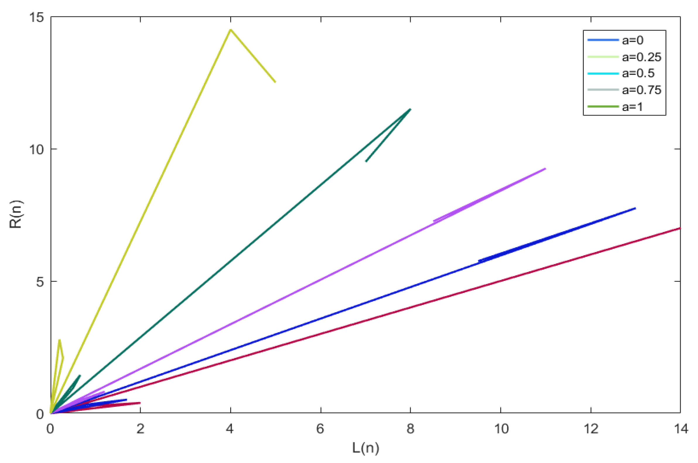
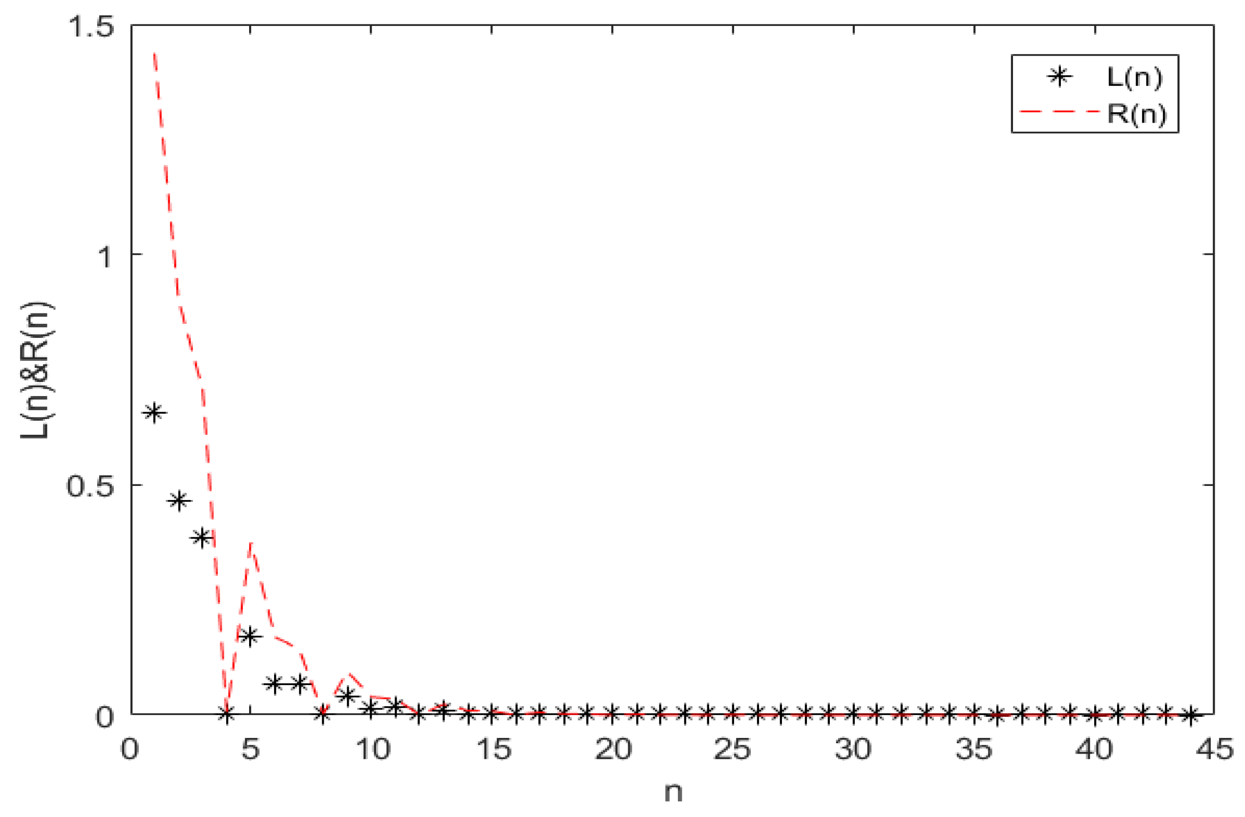
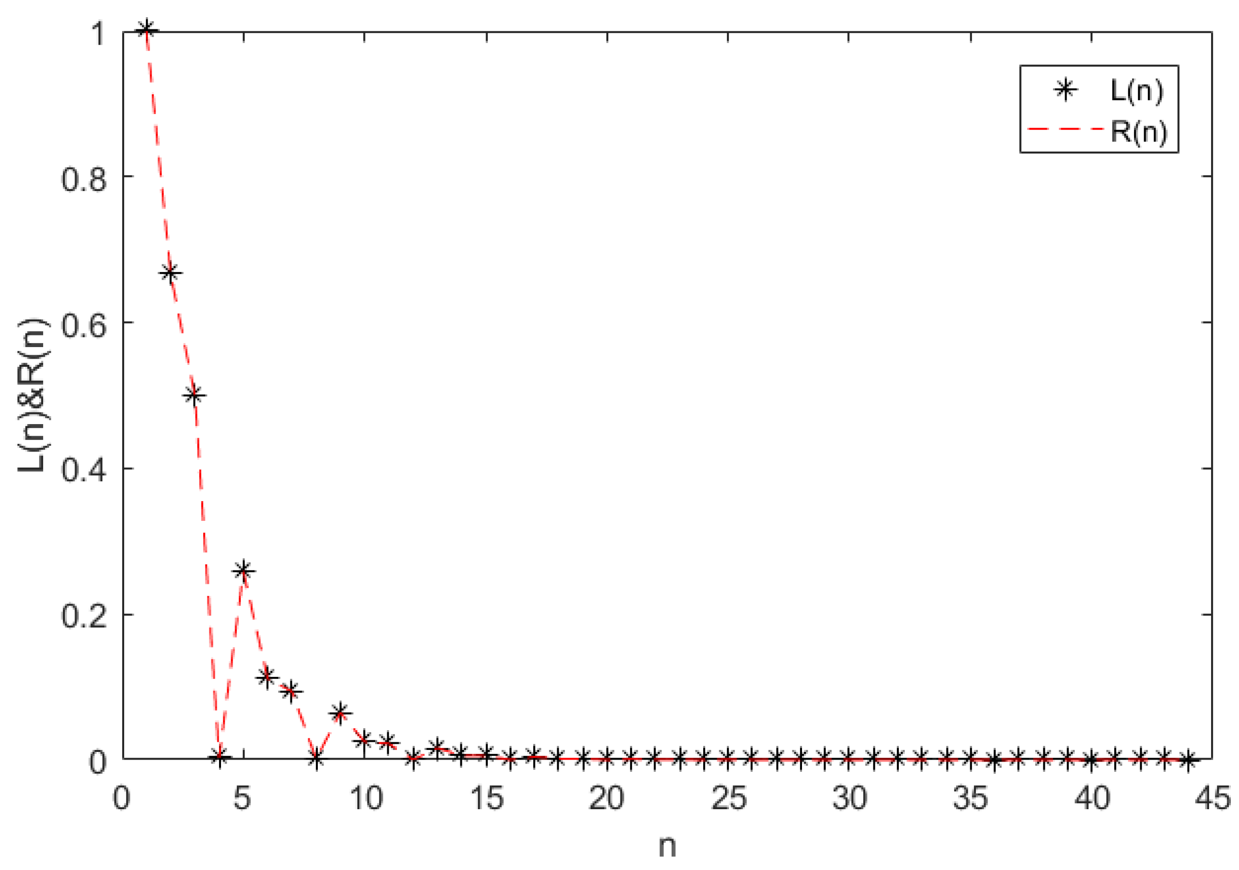
4. Numerical Example

Computer numerical simulation is helpful to better understand and observe the dynamic behavior of the fifth-order fuzzy difference Equation (9). In this section, we use the software package Matlab 2016 to carry out numerical experiments on the main conclusions obtained above. See Appendix for detailed Matlab calculation codes. As an example, we consider the following fuzzy system.

Example 1.

Consider the fuzzy system

$$x_{n+1}=\frac{A{x}_{n-1}{x}_{n-2}+B{x}_{n-3}}{D+C{x}_{n-4}},n=0,1,2,\cdots ,$$

(32)

where the parameters $A,B,C,D$ are positive trivial fuzzy numbers and the initial conditions $x_{-4},x_{-3},x_{-2},x_{-1},x_0$ are positive nontrivial fuzzy numbers. From Theorem 6, we take the parameters ${\left[A\right]}_{\alpha }=\left[A,A\right]=0.3,{\left[B\right]}_{\alpha }=\left[B,B\right]=3,{\left[C\right]}_{\alpha }=\left[C,C\right]=6,{\left[D\right]}_{\alpha }=\left[D,D\right]=12,\alpha \in \left[0,1\right]$ and the initial conditions ${\left[x_i\right]}_{\alpha }\subset \left(0,\frac{0.7D-B}{A}\right),\alpha \in \left(0,1\right)$ such that

$$x_{-4}(x)=\{\begin{array}{c}\frac{1}{2}x-\frac{1}{2},1\le x\le 3,\\ -\frac{1}{2}x+\frac{5}{2},3\le x\le 5,\end{array}{x}_{-3}(x)=\{\begin{array}{c}x-3,3\le x\le 4,\\ -x+5,4\le x\le 5,\end{array}{x}_{-2}(x)=\{\begin{array}{c}\frac{1}{2}x-1,2\le x\le 4,\\ -\frac{1}{2}x+3,4\le x\le 6,\end{array}$$

(33)

and

$$x_{-1}(x)=\{\begin{array}{c}\frac{1}{3}x-\frac{5}{3},5\le x\le 8,\\ -\frac{1}{2}x+5,8\le x\le 10,\end{array}{x}_0(x)=\{\begin{array}{c}\frac{1}{3}x-\frac{7}{3},7\le x\le 10,\\ -\frac{1}{4}x+\frac{7}{2},10\le x\le 14,\end{array}$$

(34)

Under (33) and (34), we can obtain

$${\left[x_{-4}\right]}_{\alpha }=\left[1+2\alpha ,5-2\alpha \right],{\left[x_{-3}\right]}_{\alpha }=\left[3+\alpha ,5-\alpha \right],{\left[x_{-2}\right]}_{\alpha }=\left[2+2\alpha ,6-2\alpha \right],$$

$${\left[x_{-1}\right]}_{\alpha }=\left[5+3\alpha ,10-2\alpha \right],{\left[x_0\right]}_{\alpha }=\left[7+3\alpha ,14-4\alpha \right].$$

In terms of Equation (32), we can establish the following difference symmetric system with parameter $\alpha$

$$L_{n+1,\alpha }=\frac{0.3L_{n-1,\alpha }{L}_{n-2,\alpha }+3L_{n-3,\alpha }}{12+6R_{n-4,\alpha }},R_{n+1,\alpha }=\frac{0.3R_{n-1,\alpha }{R}_{n-2,\alpha }+3R_{n-3,\alpha }}{12+6L_{n-4,\alpha }},\alpha \in \left[0,1\right],n=0,1,2,\cdots .$$

(35)

Obviously, it is known that the symmetric system (35) satisfies the condition of Theorem 6. Thus, from Theorem 6, we can obtain that the trivial solution $x=\widehat{0}$ of system (32) is uniformly asymptotically stable with respect to $D$ as $n\to \infty$. (seeFigure A1, Figure A2, Figure A3 and Figure A4). It can be clearly seen from Figure A1 that when the parameters $\alpha =0,0.25,0.5,0.75$ and 1,$\underset{n\to +\infty }{\lim }L(n)=0$ and $\underset{n\to +\infty }{\lim }R(n)=0$ as $n\to \infty$. Figure A2 shows that when the parameters $\alpha =0$, $\underset{n\to +\infty }{\lim }L(n)=0$ and $\underset{n\to +\infty }{\lim }R(n)=0$ as $n\to \infty$, Figure A3 shows that when the parameters $\alpha =0.5$, $\underset{n\to +\infty }{\lim }L(n)=0$ and $\underset{n\to +\infty }{\lim }R(n)=0$ as $n\to \infty$, and Figure A4 shows that when the parameters $\alpha =1$, $\underset{n\to +\infty }{\lim }L(n)=\underset{n\to +\infty }{\lim }R(n)=0$ as $n\to \infty$. The calculation times for obtaining Figure A1, Figure A2, Figure A3 and Figure A4 are 0.000647 s, 0.000229 s, 0.000248 s, and 0.000278 s, respectively.

5. Conclusions

In this paper, the dynamic properties of a class of fifth-order fuzzy difference system (9) are studied. Firstly, from the fuzzy sets theory, we proved that the fuzzy system (9) exists a unique positive fuzzy solution $\{x_n\}$ when the parameters $A,B,C,D$ and the initial conditions $x_{-4},x_{-3},x_{-2},x_{-1},x_0$ are positive fuzzy numbers. Secondly, the stability and instability of the fuzzy difference system (9) at equilibrium points are analyzed using linearization theory and mathematical induction. Finally, under the stability theory and inequality techniques, it is proved that the trivial solution $x=\widehat{0}$ of the fuzzy difference system (9) is uniformly asymptotically stable with respect to $D$ as $n\to \infty$ when the parameters $A,B,C,D$ are positive trivial fuzzy numbers and the initial conditions are positive fuzzy numbers with ${\left[x_i\right]}_{\alpha }\subset (0,(\epsilon D-B)/A),$ $i=-4,-3,-2,-1,0,\epsilon D>B,\epsilon \in (0,1),\alpha \in (0,1]$. In addition, numerical experiments are carried out by using the software package MATLAB 2016, and the correctness of theoretical analysis in this paper is verified.

Finally, we must highlight the limitations of our proposed approach. The method in this paper is only applicable to the case that the right-hand function of the fuzzy system is monotonic function. In our next work, we plan to further research the case that the right-hand function of the fuzzy system is nonmonotonic or abstract function.

References

1. Liao, Y.Z. Dynamics of two-species harvesting model of almost periodic facultative mutualism with discrete and distributed delays. Eng. Lett. 2018, 26, 7–13. [Google Scholar]
2. Yang, X.S.; Cao, J.D. Adaptive pinning synchronization of coupled neural networks with mixed delays and vector-form stochastic perturbations. Acta Math. Sci. 2012, 32B, 955–997. [Google Scholar]
3. Li, X.J.; Lu, S.P. Periodic solutions for a kind of high-order p-Laplacian differential equation with sign-changing coefficient ahead of the non-linear term. Nonlinear Anal.-Theory Methods Appl. 2009, 70, 1011–1022. [Google Scholar] [CrossRef]
4. Apalara, T.A. Uniform decay in weakly dissipative timoshenko system with internal distributed delay feedbacks. Acta Math. Sci. 2016, 36B, 815–830. [Google Scholar] [CrossRef]
5. Jia, X.J.; Jia, R.A. Improve efficiency of biogas feedback supply chain in rural China. Acta Math. Sci. 2017, 37B, 768–785. [Google Scholar] [CrossRef]
6. Boukhatem, Y.; Benabderrahmane, B. General decay for a viscoelastic equation of variable coefficients with a time-varying delay in the boundary feedback and acoustic boundary conditions. Acta Math. Sci. 2017, 37B, 1453–1471. [Google Scholar] [CrossRef]
7. Zhao, Z.H.; Li, Y.; Feng, Z.S. Traveling wave phenomena in a nonlocal dispersal predator-prey system with the Beddington-DeAngelis functional response and harvesting. Bound. Value Probl. Math. Biosci. Eng. 2021, 18, 1629–1652. [Google Scholar] [CrossRef]
8. Shi, Q.H.; Zhang, X.B.; Wang, C.Y.; Wang, S. Finite time Blowup for Klein-Gordon- Schrodinger System. Math. Methods Appl. Sci. 2019, 42, 3929–3941. [Google Scholar] [CrossRef]
9. Wu, Q.; Pan, C.H.; Wang, H.Y. Speed determinacy of the traveling waves for a three species time-periodic Lotka-Volterra competition system. Math. Methods Appl. Sci. 2022, 45, 6080–6095. [Google Scholar] [CrossRef]
10. Elsayed, E.M.; Harikrishnan, S.; Kanagarajan, K. On the Existence and Stability of Boundary Value Problem for Differential Equation with Hilfer-Katugampola Fractional Derivative. Acta Math. Sci. 2019, 39B, 1568–1578. [Google Scholar] [CrossRef]
11. Zheng, B.B.; Hu, C.; Yu, J.; Jiang, H.J. Synchronization analysis for delayed spatio-temporal neural networks with fractional-order. Neurocomputing 2021, 441, 226–236. [Google Scholar] [CrossRef]
12. Stević, S. Global stability and asymptotics of some classes of rational difference equations. J. Math. Anal. Appl. 2006, 316, 60–68. [Google Scholar] [CrossRef] [Green Version]
13. Muroya, Y.; Ishiwata, E.; Guglielmi, N. Global stability for nonlinear difference equations with variable coefficients. J. Math. Anal. Appl. 2007, 334, 232–247. [Google Scholar] [CrossRef] [Green Version]
14. Hu, L.X.; Xia, H.M. Global asymptotic stability of a second order rational difference equation. Appl. Math. Comput. 2014, 233, 377–382. [Google Scholar] [CrossRef]
15. Haddad, N.; Touafek, N.; Rabago, J.F.T. Well-defined solutions of a system of difference equations. J. Appl. Math. Comput. 2018, 56, 439–458. [Google Scholar] [CrossRef]
16. Agarwal, R.P.; Li, W.T.; Pang, P.Y.H. Asymptotic behavior of a class of nolinear delay difference equations. J. Differ. Equ. Appl. 2002, 8, 719–728. [Google Scholar] [CrossRef]
17. Pielou, E.C. Population and Community Ecology: Principles and Methods; Gordon and Breach: London, UK, 1975. [Google Scholar]
18. Popov, E.P. Automatic Regulation and Control; Nauka: Moscow, Russia, 1966. (In Russian) [Google Scholar]
19. Elabbasy, E.M.; Elsayed, E.M. Dynamics of a rational difference equation. Chin. Ann. Math. 2009, 30B, 187–198. [Google Scholar] [CrossRef]
20. Elsayed, E.M. On the solutions and periodic nature of some systems of difference equations. Int. J. Biomath. 2014, 7, 1450067. [Google Scholar] [CrossRef]
21. Elsayed, E.M. Expression and behavior of the solutions of some rational recursive sequences. Math. Methods Appl. Sci. 2016, 39, 5682–5694. [Google Scholar] [CrossRef]
22. Huo, H.; Li, W. Stable periodic solution of the discrete periodic Leslie-Gower predator-prey model. Math. Comput. Model. 2004, 40, 261–269. [Google Scholar] [CrossRef]
23. Anderson, D.R. Global stability for nonlinear dynamic equations with variable coefficients. J. Math. Anal. Appl. 2008, 345, 796–804. [Google Scholar] [CrossRef] [Green Version]
24. Galewski, M. A note on the existence of a bounded solution for a nonlinear system of difference equations. J. Differ. Equ. Appl. 2010, 16, 121–124. [Google Scholar] [CrossRef]
25. Chen, Y.H.; Yang, B.; Meng, Q.F.; Zhao, Y.; Abraham, A. Time-series forecasting using a system of ordinary differential equations. Inf. Sci. 2011, 181, 106–114. [Google Scholar] [CrossRef]
26. Elsayed, E.M. Behavior and expression of the solutions of some rational difference equations. J. Comput. Anal. Appl. 2013, 15, 73–81. [Google Scholar]
27. Elsayed, E.M. Solutions of rational difference systems of order two. Math. Comput. Model. 2012, 55, 378–384. [Google Scholar] [CrossRef]
28. Elsayed, E.M. Solution for systems of difference equations of rational form of order two. Comput. Appl. Math. 2014, 33, 751–765. [Google Scholar] [CrossRef]
29. Li, W.T.; Sun, H.R. Dynamics of a rational difference equation. Appl. Math. Comput. 2005, 163, 577–591. [Google Scholar] [CrossRef]
30. Saleh, M.; Abu-Baha, S. Dynamics of a higher order rational difference equation. Appl. Math. Comput. 2006, 181, 84–102. [Google Scholar] [CrossRef]
31. Dehghan, M.; Mazrooei-Sebdani, R. Dynamics of a higher-order rational difference equation. Appl. Math. Comput. 2006, 178, 345–354. [Google Scholar] [CrossRef]
32. Zayed, E.M.E.; El-Moneam, M.A. On the global asymptotic stability for a rational recursive sequence. Iran. J. Sci. Technol. Trans. A Sci. 2012, 35, 333–339. [Google Scholar]
33. Chrysafifis, K.A.; Papadopoulos, B.K.; Papaschinopoulos, G. On the fuzzy difference equations of finance. Fuzzy Sets Syst. 2008, 159, 3259–3270. [Google Scholar] [CrossRef]
34. Zhang, Q.H.; Liu, J.; Luo, Z. Dynamical behavior of a third-order rational fuzzy difference equation. Adv. Differ. Equ. 2015, 2015, 108. [Google Scholar] [CrossRef] [Green Version]
35. Hatir, E.; Mansour, T.; Yalcinkaya, I. On a fuzzy difference equation. Util. Math. 2014, 93, 135–151. [Google Scholar]
36. Khastan, A. Fuzzy logistic difference equation. Iran. J. Fuzzy Syst. 2018, 15, 55–66. [Google Scholar]
37. Papaschinopoulos, G.; Stefanidou, G. Boundedness and asymptotic behaviour of the solutions of a fuzzy difference equation. Fuzzy Sets Syst. 2003, 140, 523–539. [Google Scholar] [CrossRef]
38. Khastan, A. New solutions for first order linear fuzzy difference equations. J. Comput. Appl. Math. 2017, 312, 156–166. [Google Scholar] [CrossRef]
39. Allahviranloo, T.; Salahshour, S.; Khezerloo, M. Maximal-and minimal symmetric solutions of fully fuzzy linear systems. J. Comput. Appl. Math. 2011, 235, 4652–4662. [Google Scholar] [CrossRef] [Green Version]
40. Kocic, V.L.; Ladas, G. Global Behavior of Nonlinear Difference Equations of Higher Order with Applications; Kluwer Academic: Dordrecht, The Netherlands, 1993. [Google Scholar]
41. Kulenovic, M.R.S.; Ladas, G. Dynamic of Second-Order Rational Difference Equations: With Open Problems and Conjectures; Chapman & Hall CRC Press: Boca Raton, FL, USA, 2001. [Google Scholar]
42. Camouzis, E.; Ladas, G. Dynamics of Third-Order Rational Difference Equations: With Open Problems and Conjectures; Chapman and Hall/CRC: Boca Raton, FL, USA, 2007. [Google Scholar]
43. Deeba, E.Y.; De Korvin, A.; Koh, E.L. A fuzzy difference equation with an application. J. Differ. Equ. Appl. 1996, 2, 365–374. [Google Scholar] [CrossRef]
44. Deeba, E.Y.; De Korvin, A. Analysis by fuzzy difference equations of a model of CO2 level in the blood. Appl. Math. Lett. 1999, 12, 33–40. [Google Scholar] [CrossRef] [Green Version]
45. Zhang, Q.H.; Yag, L.; Liao, D. Behavior of solutions to a fuzzy nonlinear difference equation. Iran. J. Fuzzy Syst. 2012, 9, 1–12. [Google Scholar]
46. Zhang, Q.H.; Yang, L.; Liao, D. On first order fuzzy Ricatti difference equation. Inf. Sci. 2014, 270, 226–236. [Google Scholar] [CrossRef]
47. Wang, C.Y.; Su, X.L.; Liu, P.; Hu, X.H.; Li, R. On the dynamics of a five-order fuzzy difference equation. J. Nonlinear Sci. Appl. 2017, 10, 3303–3319. [Google Scholar] [CrossRef] [Green Version]
48. Khastan, A.; Alijani, Z. On the new solutions to the fuzzy difference equation xn+1=A+B/xn. Fuzzy Sets Syst. 2019, 358, 64–83. [Google Scholar] [CrossRef]
49. Zhang, Q.H.; Lin, F.; Zhong, X. On discrete time Beverton-Holt population model with fuzzy environment. Math. Biosci. Eng. 2019, 16, 1471–1488. [Google Scholar] [CrossRef]
50. Bede, B. Mathematics of Fuzzy Sets and Fuzzy Logic; Springer: London, UK, 2013. [Google Scholar]
51. Diamond, P.; Kloeden, P. Metric Spaces of Fuzzy Sets; World Scientific: Singapore, 1994. [Google Scholar]
52. Sedaghat, H. Nonlinear Difference Equations: Theory with Applications to Social Science Models; Kluwer Academic Publishers: Dordrecht, The Netherlands, 2003. [Google Scholar]
53. Zhang, Q.H.; Lin, F. On dynamical behaviour of discrete time fuzzy logistic equation. Discret. Dyn. Nat. Soc. 2018, 2018, 8742397. [Google Scholar]
54. Papaschinopoulos, G.; Papadopoulos, B.K. On the fuzzy difference equation xn+1=A+xn/xnm. Fuzzy Sets Syst. 2002, 129, 73–81. [Google Scholar] [CrossRef]
55. Wu, C.X.; Zhang, B.K. Embedding problem of noncompact fuzzy number space (I). Fuzzy Sets Syst. 1999, 105, 165–169. [Google Scholar] [CrossRef]
56. Lakshmikantham, V.; Vatsala, A.S. Basic theory of fuzzy difference equations. J. Differ. Equ. Appl. 2002, 8, 957–968. [Google Scholar] [CrossRef]
Publisher’s Note: MDPI stays neutral with regard to jurisdictional claims in published maps and institutional affiliations.