
Recent Advances in Surrogate Modeling Methods for Uncertainty Quantification and Propagation


1
Institute of Solid Mechanics, Beihang University, Beijing 100191, China
2
Faculty of Mechanical Engineering & Mechanics, Ningbo University, Ningbo 315211, China
3
Department of Mechanical Science and Engineering, Technische Universität Dresden, Holbeinstraße 3, 01307 Dresden, Germany
*
Author to whom correspondence should be addressed.
Symmetry 2022, 14(6), 1219; https://doi.org/10.3390/sym14061219
Submission received: 7 May 2022
/
Revised: 29 May 2022
/
Accepted: 10 June 2022
/
Published: 13 June 2022
(This article belongs to the Special Issue Advances in Computational Mechanics for Symmetrical Engineering Systems)
Abstract
:Surrogate-model-assisted uncertainty treatment practices have been the subject of increasing attention and investigations in recent decades for many symmetrical engineering systems. This paper delivers a review of surrogate modeling methods in both uncertainty quantification and propagation scenarios. To this end, the mathematical models for uncertainty quantification are firstly reviewed, and theories and advances on probabilistic, non-probabilistic and hybrid ones are discussed. Subsequently, numerical methods for uncertainty propagation are broadly reviewed under different computational strategies. Thirdly, several popular single surrogate models and novel hybrid techniques are reviewed, together with some general criteria for accuracy evaluation. In addition, sample generation techniques to improve the accuracy of surrogate models are discussed for both static sampling and its adaptive version. Finally, closing remarks are provided and future prospects are suggested.
1. Introduction
Practical engineering structures are inevitably rife with diverse types of uncertainties related to model assumption, material property, loads, boundary conditions, etc. In general, these uncertainties can be classified into two categories: aleatory uncertainty and epistemic uncertainty [1]. In this context, aleatory uncertainty reveals the inherent variation in the system and is irreducible but can be described by a probability distribution. However, epistemic uncertainty reflects a lack of knowledge of the system and is reducible if more information is procured. Tackling these uncertainties in an effective manner has become a critical consideration for both practitioners and academicians.
Uncertainty quantification is a route of the quantitative representation of and reduction in uncertainties in both simulation and practical applications. With the perquisite of sufficient samples, the probabilistic model has always been the most popular scheme to tackle the aleatory uncertainty [2,3]. For those scenarios with scarce samples, various representative non-probabilistic theories have been developed for the treatment of epistemic uncertainty, including fuzzy theory, interval theory, convex models, evidence theory, and so on [4]. Apart from the traditional schemes, several recent studies have also suggested a more applicable hybrid framework to tackle coexisting uncertainties in engineering systems with increasing complexity [5,6,7].
As another important issue in uncertainty treatment, uncertainty propagation focuses on characterizing the impact of fluctuations in the input parameters on system responses. Compared with the probability distribution function, some easy-to-procure indicators, e.g., the statistical moments of response, are more applicable in engineering practices [8]. To this end, various numerical methods have flourished and have been successfully applied in structural stochastic response analysis, reliability analysis, robust design, multidisciplinary optimization, etc. [9,10,11]. As the complexity of simulation models grows, however, the corresponding computational cost of these conventional numerical methods becomes increasingly unaffordable.
To alleviate the computing burden, the surrogate model (also known as the metamodel) has been an attractive alternative, wherein a cheap-to-run approximation model is constructed to replace the original time-consuming high-fidelity simulation. Until now, various surrogate models and auxiliary optimization algorithms have been developed to deliver better predictions [12,13]. In addition to pursuing a more accurate surrogate model, selecting appropriate samples is another way to help enhance the prediction accuracy, and thus the literature on sampling strategies of the surrogate model has also seen a rapid increase in recent decades [14].
This paper aims to provide a general review of the advances in both uncertainty treatment and the surrogate model in the past two decades. The remainder of this paper is organized as follows. Firstly, mathematical models for uncertainty quantification, including probabilistic, non-probabilistic and hybrid ones, are discussed in Section 2. In Section 3, numerical methods are divided into four categories to address their differences in uncertainty propagation. Section 4 presents several popular surrogate models and their hybrid strategies successively, together with a range of commonly used criteria for accuracy evaluation. For sampling strategies in surrogate modeling, Section 5 discusses the one-shot and sequential ones, respectively. Finally, Section 6 closes the paper by encapsulating the main points and concluding remarks.
2. Mathematical Models in Uncertainty Quantification
In this section, various uncertainty modeling techniques, including probabilistic, non-probabilistic and hybrid methods, are reviewed with a focus on their recent advances. Since probabilistic methods have been well studied and applied in engineering scenarios, the invariant/time-variant/space-variant characteristics of random parameters are summarized and discussed in this section. As a series of attractive tools in measuring the uncertainties with insufficient information, existing non-probabilistic methods are subsequently discussed, together with their fundamentals. Finally, hybrid strategies concerning multiple uncertain modeling techniques are classified with a closing review.
2.1. Probabilistic Models
Under the probabilistic framework, as shown in Figure 1, the statistical characteristic of uncertain parameters can be described by random variables, stochastic process or random fields [15]. The probability density functions (PDF) with different colors in Figure 1a illustrate the impact of Gaussian distribution parameters on random variables. Considering the time-/space-varying characteristics of the random variable, stochastic process and random fields are displayed in Figure 1b and 1c, respectively. According to the probability theory, a random variable defined on the probability triple maps a random event to real value in [15]. For brevity but without loss of generality, a collection of random variables can be exploited to represent the stochastic process or random field, where is the index indicating time or position, respectively.
For many random parameters measured in engineering practices, such as geometry size, material properties and loads applied to structures, there are inevitably small fluctuations in their observed values. When sufficient samples are provided, the accurate PDF of these random variables can be easily procured to quantify their uncertainties. There are a variety of probability distributions widely adopted in engineering practices, including Gaussian, Poisson, and Weibull distributions [16,17,18,19]. For multidimensional random variables, the easy-to-procure incomplete information such as statistical moments and marginal probability distributions, instead of the precise joint probability distribution, is often exploited to measure the randomness of parameters. To obtain the above statistical information, many probabilistic methods have been widely adopted, such as Nataf transformation and the Copula function [20,21]. Based on data-driven strategies, emerging machine learning-aided techniques also provide an attractive alternative for uncertainty quantification [22,23]. As an extension of deterministic finite element method (FEM), the stochastic FEM has been regarded as a powerful approach when solving the problems with random properties [24].
Due to the changing environmental factors, the uncertainty of parameters often has time-varying characteristic in many practical problems, such as the aerodynamic heat on hypersonic vehicles and wind excitations of buildings [25,26]. In this context, the stochastic process model can be employed to conduct uncertainty modeling for these time-varying parameters. To approximate the stochastic process, many methods have been developed to simulate Gaussian or non-Gaussian and stationary or non-stationary processes [27,28]. The Markov process, which describes the transitions between a sequence of states, plays an increasingly important role in system survival/failure behavior evaluation [29]. In addition, recent investigations have shown the potential of data-driven methods in simulating the statistical properties of stochastic processes [30].
In addition to the above two descriptions, some researchers have also noticed that many parameters vary with spatial locations in practical cases, such as the mechanical properties of geotechnical materials and composite structures [31,32]. In this context, this spatially distributed uncertainty can be statistically described by means of random fields. To simulate the spatial-varying uncertainty, various random field discretization techniques have been applied in geotechnical engineering and structural vibration analysis, such as local average subdivision, turning-band methods, and Karhunen–Loève (KL) expansion [31,33,34,35]. The stochastic spectral element method (SEM) has also been proven to be a powerful approach to tackle the spatial uncertainty in dynamic systems [36,37,38]. The success of machine learning techniques is also spreading their application to random fields [39].
2.2. Non-Probabilistic Models
Probabilistic approaches have offered a stable framework for uncertainty analysis, with the premise that sufficient experimental samples are available to construct the precise probability distribution of uncertain parameters. However, the experimental conditions or costs of many practical engineering problems often restrict the acquisition of adequate data, which further leads to the inapplicability of the probabilistic method [40,41]. To procure more credible results for engineering problems with insufficient data, many non-probabilistic methods have flourished in recent decades, providing an attractive framework for uncertainty analysis.
Fuzzy set theory. In a large number of real-world problems, the relationship between elements and sets is sometimes vague, and it is difficult to give a crisp partition. Conventional set theory exploits the binary to describe the degree of an element with respect to the set . In contrast, fuzzy set theory leverages a real number in the closed interval to quantitatively measure this affiliation degree more precisely. On this basis, the fuzzy set can be defined as
where the superscript ‘’ is the symbol of fuzzy set; the reference set is called the universe of discourse; the real-valued function is called a membership function; represents the membership degree of element to the fuzzy set . The techniques used to generate the membership function have received extensive investigations, and there are many widely used membership functions such as Gaussian, triangular and trapezoidal functions [42]. In addition to the conventional fuzzy sets, many extended fuzzy sets such as intuitionistic and hesitant ones have emerged in recent decades [43,44]. Considering the time-variant properties in some fuzzy variables, many scholars have also begun to focus on the time-dependent fuzzy uncertainty [45,46]. With its high degree of maturity, fuzzy set theory has been extensively applied in structural response analysis, reliability assessment, parameter identification, etc. [45,47,48].
Interval theory. In many engineering problems, the values of external loads or material properties often fluctuate within a certain range. With interval theory, these uncertain-but-bounded parameters can be described as follows
where denotes the interval vector composed of interval variables; and are called the lower and upper bound of the interval variable , respectively; and and are the midpoint and the radius of , respectively. Since the interval model only needs the bounds of the parameters to quantify the uncertainty, it has been widely applied in various engineering fields [49,50,51]. Similar to the probabilistic methods, existing interval-related studies can also be divided into those on interval variables [49], interval process [52] and interval fields [51].
Ellipsoid model. To remedy the deficiency that the interval model can only handle independent variables, the ellipsoid model has been applied to tackle various engineering problems with dependent variables [41,53,54]. The explicit mathematical formula to represent the ellipsoid model is given as follows
where stands for the variable vector in m-dimensional space; and are the characteristic matrix and the centroid of the ellipsoid, respectively; and the characteristic matrix measures the shape and orientation of the ellipsoid. When conducting the ellipsoid-based uncertainty quantification, the optimal ellipsoid model is considered to envelop all experimental samples with a minimal volume. In this context, many ellipsoid-modeling techniques have flourished, such as the rotation matrix method, the correlation approximation method and data-driven methods [55,56,57,58]. Theoretically, efficiently constructing a reasonable ellipsoid model under high-dimensional space remains a challenging issue.
Evidence theory. The evidence theory, also known as Dempster–Shafer theory, has seen increasing applications due to its advantages in flexibly, dealing with imprecise and incomplete uncertain information from multiple sources [59,60,61]. Two important measures, i.e., belief and plausibility, are considered in the evidence theory for each proposition in the frame of discernment :
where is interpreted as the basic probability assignment (BPA) of possible proposition ; denotes the aggregate of values that totally support the proposition ; represents the aggregate of values that totally or partially support the proposition . Generation techniques of BPA, which play a key role in practical applications, have also received extensive investigations [62]. Considering that existing evidence inevitably conflicts in multi-source information, ways of measuring and fusing these inconsistencies more reasonably have been a research focus in recent decades [63].
Rough set theory. Rough set theory is recognized as a promising technique for uncertainty management, especially for those uncertainties with incomplete and inconsistent information. By exploiting a boundary region of a set, the classical rough set theory defines the following two operations to express vagueness:
where is an equivalence relation (also known as indiscernibility relation) on the universe ; is an arbitrary element in a subset ; and are named the -lower and -upper approximations of , respectively. As the above equivalence relations are too stringent, many scholars have proposed more general rough sets (e.g., probabilistic-rough, fuzzy-rough and rough-soft sets) for engineering applications [64,65,66]. The rough set model has been widely applied in decision making, attribute reduction and fault diagnosis [65,67,68].
In addition to the above models, other types of non-probabilistic methods have also been developed in terms of various requirements for uncertainty modeling, such as possibility theory (see [69]), the information gap model (see [70]), the parallelepiped model (see [71]), the super ellipsoid model (see [72]) and the convex polyhedral model (see [73]). To intuitively exhibit the characteristic of different non-probabilistic convex modeling techniques in uncertainty quantification, the envelope results of experimental samples under five types of convex models are shown in Figure 2.
2.3. Hybrid Models
Overall, significant studies have investigated uncertainty quantification based on both probabilistic and non-probabilistic schemes. In some engineering practices, however, diverse types of uncertainty often coexist in a unified system, and using conventional single-type models becomes incompetent [2,40,74]. In this context, a variety of hybrid uncertainty modeling strategies have been increasingly attended and investigated in recent years. Theoretically, they can be divided into two categories: parallel and embedded hybrid methods. As a common hybrid case, parallel-type hybrid methods enable different uncertain parameters exist in systems simultaneously and independently. In contrast, the embedded-type ones are more general when dealing with various coexisting uncertainties but also remain technically challenging at the same time [40,75]. For a better understanding, Table 1 summarizes related investigations on the above hybrid strategies in past five years.
Take the probabilistic-interval hybrid model as an example; the parallel type is suitable for those problems with determined probability distribution types but inaccurate parameter values. In contrast, the embedded type is suitable for solving problems where only the fluctuation intervals can be obtained for some parameters due to the lack of available samples or expert experience. In practice, it is usually strenuous to choose the most reasonable hybrid strategy for a certain problem and the selection criteria of these two types of hybrid models have not been reported. With the increasing complexity of uncertainties in multidisciplinary practices, the study of engineering problems concerning more than two kinds of uncertainties under a unified framework is promising but mostly unexplored [3,5].
3. Numerical Methods in Uncertainty Propagation
After the results of uncertainty quantification are obtained, the next priority is to measure the impact of disturbances in the input parameters on the system responses, i.e., uncertainty propagation. In this section, several popular numerical methods in uncertainty propagation are reviewed, including sampling-based, expansion-based, optimization-based and integration-based ones. They are schematically summarized in the following subsection.
3.1. Sampling-Based Method
Sampling-based techniques predominantly include Monte Carlo simulation (MCS) and its variants. As shown in Figure 3, MCS generates random variables from probability density functions to estimate unknown parameters and then calculate their expected value and variances. Based on the law of large numbers and the central limit theorem, one usually works with the multivariable normal distribution. In practice, the MCS procedure remains in essence identical regardless of the complexity or the computational burden of the simulation model. Theoretically, MCS requires extensive samplings (usually 106 runs or greater) to procure reliable statistics, which implies that it is often computationally expensive for complex engineering problems [84]. By updating a Markov chain with desired distribution as the stationary distribution, the Markov Chain Monte Carlo (MCMC) method aims to recover the properties of an unknown probability distribution and is deemed an important complement to the problems with known probability distribution. Both MCS and MCMC have been widely applied to obtain reliable results in various domains [85,86,87].
Another important family of Monte Carlo techniques is importance sampling (IS) and its adaptive version (AIS). As a variance reduction technique, IS utilizes a targeted sampling strategy to reduce the number of model evaluations. In contrast, AIS focuses on employing the information of previously drawn samples to adjust proposals to further reduce the variance in the desired estimators. For applications of importance sampling in reliability analysis, one can consult [89,90,91].
3.2. Expansion-Based Method
The perturbation method (also known as the small-parameter expansion method) expresses the desired solution in terms of a formal power series (i.e., perturbation series) in small parameter that measures the deviation from the fully solvable problem [92]. A pivotal idea of this method is an intermediate operation that breaks the problem into ‘solvable’ and ‘perturbative’ parts. On this basis, the full solution can be subsequently represented by a series in with the first-order perturbative correction:
where and indicate the know solution and the first-order terms, respectively, and denotes the truncation error of high-order terms. As the basis of other expansion methods, parameter and subinterval perturbation strategy have been widely applied in heat transfer, structural-acoustic systems, etc. [6,93,94].
The Taylor series expansion method expands the system function at a certain point and constructs a polynomial using each order’s partial derivative to approximately replace the original system function [95]. Due to its implementation-friendly characteristic, the first-order Taylor series expansion has been extensively used, in which the high-order terms are truncated:
where indicates the dimension of the uncertain variable vector and and are the ith components of and , respectively. In practice, the first-order Taylor series is widely used to reduce the computational cost in heat conduction, structural vibration analysis, etc. [96,97].
The truncated Neumann series can be employed for approximate matrix inversion by introducing a liner operator [98]. The inverse of a matrix can be approximately written as:
where and satisfies the norm condition; and are the inverse of and the identity matrix, respectively; and the Neumann series is truncated with n terms. Neumann series have been employed to approximate the interval matrix inverse in acoustic field, coupled structural-acoustic field prediction, etc. [99,100].
Karhunen–Loève (KL) expansion represents the stochastic process as an infinite linear combination of orthogonal functions, similar to the Fourier series representation of functions on a bounded interval [27,101]. Assume that is a zero-mean square-integrable stochastic process defined over the probability space on a closed interval and admits the following decomposition:
where are pairwise uncorrelated random variables and the real-valued functions are continuous on that are pairwise orthogonal in . KL expansion has been widely applied in dynamic uncertainty analysis, including stochastic process, random field models and interval process [101,102,103].
3.3. Optimization-Based Method
According to the type of uncertain variables involved, existing optimization-based methods in uncertainty propagation can be broadly classified into three main categories: stochastic programming, fuzzy programming and interval optimization [104].
Stochastic programming combines conventional deterministic optimization with random variables and probabilistic constraints, which often require time-consuming simulations [105]. Such problems can be calculated by either classical methods, such as nonlinear programming or quadratic programming, or other advanced methods, e.g., Nondominated Sorting Genetic Algorithm II (NAGA-II) or simulated annealing (SA) optimization [106,107,108].
Fuzzy programming broadly includes two main concerns: the possibilistic programming approach, using the possibility or necessity measures to convert the fuzzy mathematical programming problems into conventional ones, and the ordering-based approach, considering non-dominated solutions based on the ordering of fuzzy sets [109]. Many heuristic algorithms have been introduced in a variety of non-deterministic problems with fuzzy numbers, such as Particle Swarm Optimization (PSO), Ant Colony Optimization (ACO), and Genetic Algorithm (GA) [110,111,112,113].
Interval optimization transforms the non-deterministic optimization problem into a deterministic, double-loop nested optimization problem. The outer optimizer is adopted to search the optimal design variable, while the inner optimizer is employed to compute the bounds of uncertain objective functions and constraints [114]. Though such processing has high precision, it suffers from expensive computational cost. For the consideration of efficiency, various approaches have been introduced to decouple the nested optimization into a single-layer one, including the degree of interval constraint violation (DICV) [115], the Karush–Kuhn–Tucker (KKT) condition [116], lightning attachment procedure optimization (LAPO) [117], affine arithmetic [118], etc.
In addition to the above uncertainty, optimization methods can also be incorporated into ellipsoid models [119], evidence theory [120], etc. Moreover, optimization schemes have received increasing applications in hybrid uncertainties, e.g., probabilistic-interval [121], probabilistic-fuzzy [122], and interval-fuzzy uncertainties [123].
3.4. Integration-Based Method
When determining the statistical moments of performance function, analytical solutions are often strenuous to obtain. In this context, various numerical integration methods are introduced to estimate the probability distribution of the system response. In general, the statistical moments of system response can be measured in two numerical manners: the point estimation method (PEM) and the dimension-reduction method (DRM).
For the first type, the statistical moments are evaluated by the weighted sum of values of the response functions at a set of collection points in random space. Appropriate strategies for selecting the computational nodes have been increasingly investigated to enhance computational efficiency. The simplest scheme is the full factorial numerical integration (FFNI) method, which utilizes a tensor product based on the one-dimensional quadrature rule. As the number of dimensions grows, however, it suffers from the well-recognized ‘curse of dimensionality’ [124]. In this context, the sparse grid numerical integration (SGNI) method constructed by the Smolyak algorithm is more popular in engineering problems [125]. In addition, several innovative techniques, e.g., adaptive SGNI [126], high-order unscented transformation [127], cubature formulation [128] and the quasi-symmetric point method [129], have also been developed for efficiency consideration. In such cases, considerable computing efforts are usually required on high-dimensional problems.
For the second type, the multiple-dimension integral is decomposed into a sum of several low-dimensional integrals. The univariate dimension-reduction method (UDRM) [130], the eigenvector UDRM [131] and the multiplicative UDRM (M-UDRM) [132] are considered the most popular ones due to their simplicity and efficiency in moderate nonlinear problems where few performance function calls are required. For the system with large random variations and high nonlinearity, multivariate DRM (e.g., the bivariate [133] and the trivariate DRM [134]) and adaptive DRM [135] can be employed to enhance the accuracy of the evaluation of moments. Although the above significant improvements have been achieved, the scheme that can strike a trade-off between accuracy and efficiency is still of great interest in the assessment of statistical moments.
State-of-the-art numerical simulations often involve complex mechanisms with a vast number of input parameters, where extensive runs of computational models incur unaffordable computing effort in many practical cases. In view of this issue, the surrogate model has been recognized as an attractive alternative to reduce the computing budget and has received sustained attention and wide applications in recent decades. Herein, two main concerns of the surrogate model—theoretical basis and sampling strategy—are discussed in the following two sections.
4. Theoretical Basis of Surrogate Model
Surrogate models are a series of easy-to-evaluate mathematical models that approximate the original time-consuming simulation models based on paired input–output experimental samples [41]. In this section, commonly used approaches for surrogate modeling are discussed with an emphasis on their recent advances. As one of the hotspots in surrogate models, state-of-the-art hybrid strategies are subsequently discussed. Finally, several popular accuracy evaluation criteria for the surrogate model are reviewed.
4.1. Commonly Used Surrogate Model
Polynomial response surface (PRS) model. This popular model is trained by the least-square method, which minimizes the variance of unbiased estimators of the coefficients by means of the conditions of the Gauss–Markov theorem. A typical second-order PRS model can be expressed as:
where and denote the ith and the jth components of the n-dimensional design variable, respectively; is the constant term;, , stands for the coefficient of first-order term, the second-order term and the cross term, respectively.
When establishing the PRS model, the coefficients are interpreted as the significance of different terms. The remarkable smoothing capability of PRS model enables the fast convergence of noisy functions. Although the PRS model is simple and implementation-friendly, a main drawback lies in its applications for high nonlinear problems. In such cases, a vast number of samples are usually required to estimate the coefficients of PRS model, and high-order polynomials may cause instabilities. In practice, linear and second-order PRS model are commonly used ones.
Radial basis function (RBF) model. The RBF model exploits linear combinations of radial symmetric kernel functions to approximate the system function. A general RBF model can be expressed as:
where is the number of sample points; denotes the Euclidean distance between predicted point and observed point ; represents the radial basis function on ; stands for the weight coefficient to be determined. A typical structure of RBF neural network is displayed in Figure 4. Here, and denote the input and output sample respectively.
By substituting all observed sample points into Equation (11), a group of equations related to the unknown weight coefficients can be obtained
where denotes the response at the observed point , calculated by the original system function. RBF model is usually employed to interpolate scattered multivariate data and has shown satisfactory approximations for arbitrary forms of response functions. Various radial basis functions, e.g., linear, Gaussian and multi-quadric [71], can be flexibly determined for diverse practical requirements.
Polynomial chaos expansion (PCE) model. The PCE model aims to project the random variable onto a stochastic space spanned by a set of orthogonal polynomial basis. Then, a prototypical p-order PCE for an m-dimensional random variable is represented as [60]:
where denotes the polynomial basis function; is the unknown expansion coefficient vector; is calculated by ; the total number of expansion terms is .
Classical families of orthogonal polynomials have been developed and extensively used, such as Hermite, Legendre, Laguerre and Jacobi polynomials [137]. Different types of orthogonal polynomials are shown in Table 2. In practice, both generalized polynomial chaos (gPC) and arbitrary polynomial chaos (aPC) frameworks have also seen a promising future in various engineering practices with different probability measures [138].
Kriging model. The Kriging, also known as Gaussian process regression, is an interpolation methodology based on Gaussian processes governed by prior covariance, as shown in Figure 5. A general form of Kriging can be formulated as a summation of two components: a trend of mean prediction determined by several basis functions at known locations and a random error with zero-mean distribution [139]:
where and are the ith basis function and its corresponding coefficient, respectively; is the number of sample points; and denotes a Gaussian process with a zero-mean and covariance function formulated as
where stands for the variance of and is the correlation function between and with hyper-parameters .
Kriging starts with a prior distribution over functions, and a set of spatial-related observation values are then obtained. By combining the Gaussian prior with a Gaussian likelihood function for each observed value, unknown value can be predicted at new spatial locations, together with their means and covariance. The correlation function can be specified with various forms, including linear, exponential, Gaussian, etc. According to the various stochastic process assumed, there are different types of Kriging models, namely, ordinary, simple, universal Kriging, their adaptive versions, etc. [141].
Support vector regression (SVR) model. The SVR model is a supervised machine learning model and is regarded as a special version of the support vector machine for regression. SVR utilizes the kernel function to map the original data onto a high-dimensional feature space and then searches the optimal regression function in a linear feature space. A general form of the SVR model is a sum of basis function , with weighting coefficient , added to a constant term , which can be written as:
This form of SVR is similar to that of the RBF and the Kriging model. However, the way to calculate the unknown parameters in SVR model differs significantly from them. The purpose of SVR is to find a function that can estimate the output value with a deviation less than from the real value. The corresponding band of deviation is called the -tube. The optimal regression function is determined by formulating a mathematical optimization problem:
where is a linear version of SVR, denotes the predicted value, slack variables and allow the existence of outliers outside the -tube, and the regularization constant (also known as penalty coefficient) here achieves a trade-off between the model complexity and the empirical risk. For better understanding, a typical SVR model is shown in Figure 6.
Artificial neural network (ANN) model. ANNs are computational systems inspired by biological central neural networks and are gaining increasing popularity for surrogate modeling. In accordance with the universal approximation theorem, a three-layer ANN with a non-linear activation function is able to approximate any complex non-linear functions with satisfactory accuracy [142]. A typical three-layer feedforward ANN, which is trained by error back propagation algorithm, consists of an input layer, a hidden layer and an output layer, as shown in Figure 7.
The training process of an ANN mainly includes two stages: (1) signal forward propagation, in which each neuron collects incoming signals and the weighted summation of inputs is processed and transferred to the next layer of neurons by means of the activation function, and (2) error backward propagation, in which the deviation between the actual outputs and the forecasting outputs is calculated and back-propagated and then connection weights are updated by the gradient-descent strategy. Since machine learning techniques are increasingly important in many engineering fields, more complex ANNs have also received increasing applications in surrogate modeling, such as long short-term memory (LSTM), convolutional neural networks (CNNs) and deep neural networks (DNNs) [143,144,145].
4.2. Hybrid Strategies of Surrogate Model
Although an individual surrogate model can achieve good performance for certain problems, it is well recognized that no single surrogate model always performs the best for all types of engineering applications [146]. This motivates the idea of using a hybrid surrogate model that takes full advantage of the individual surrogate model to guarantee the accuracy and robustness of the predictions for diverse low-/high-dimensional problems. The basic principle of the hybrid surrogate model is to utilize a linearly weighted summation of the individual surrogate model as follows:
where is the response predicted by the hybrid surrogate model at point , is the number of surrogate models involved and is the weight associated with the ith surrogate model . Theoretically, the adjustable weights provide a flexibility to place more emphasis on the good surrogate model and less emphasis on the bad surrogate model as per the need [13].
According to the schemes for determining the weights, existing hybrid strategies can generally be classified as average measures (or global ensemble) and pointwise ones (or local ensembles) [147]. The weights evaluated by average measures remain constant in the whole design space [148,149]. However, the precision of the individual surrogate model may change significantly in the design space; accordingly, the hybrid surrogate model with fixed weights inevitably encounters a precision fluctuation. In contrast, pointwise measure-based schemes have shown more satisfactory precision, and various approaches have flourished to reasonably determine the weights, such as minimal prediction error-based, cross validation-based, optimization-based and trust region-based approaches [146,150,151,152,153,154]. In general, auxiliary optimization procedures that are used to search for the weights also inevitably increase the computing effort, especially for high-dimensional problems.
To mitigate the computational burden in complex engineering practices, building a multi-fidelity (also known as variable-fidelity) surrogate model that combines a cheaper, low-fidelity model and a more expensive, high-fidelity model has gradually become another attractive alternative [155,156]. In such cases, the global trend of the system function is captured by the low-fidelity model, and the local accuracy is guaranteed by the high-fidelity model, as shown in Figure 8. Two main concerns, including the sampling strategy and the precision combination, have always been the work emphasis under various multi-fidelity modeling frameworks.
To address the uncertainties in multi-level systems, a series of multi-level surrogate modeling strategies have also emerged to simultaneously tackle different models. When constructing a multi-level surrogate model, some scholars prefer to employ a local exploration to modify the global surrogate model [157,158], while others focus on tackling the challenge of co-existing uncertainties in surrogate modeling [159,160,161].
4.3. Accuracy Evaluation of a Surrogate Model
To assess the accuracy of a surrogate model, different metrics can be used to measure the deviation between the predicted value and the actual value from the following perspectives.
Coefficient of determination . The is used to gauge the overall reliability of the surrogate model, which can be written as:
where and denote the actual value, the predicted value, the mean of the actual value and the number of test samples, respectively. In general, the larger the is, the higher the accuracy of surrogate model is.
Mean square error (MSE). The MSE utilizes the square of Euclidean distance to measure the prediction error, and it is defined as:
Since the MSE does not have the same unit of measurement as the actual value, its square root version (root mean square error, RMSE) provides a more intuitive measurement:
Theoretically, both the MSE and the RMSE stay at positive values and decrease as the prediction error approaches zero.
Mean absolute error (MAE). The MAE describes the average deviation between the predicted value and actual value and is defined as:
Relative average absolute error (RAAE). The RAAE is utilized to measure the global relative error, and it can be expressed as:
5. Sampling Strategy of Surrogate Model
Sampling (also known as Design of Experiments, DoE), the process of generating a good set of data points in the design space, has become a pivotal issue in experiments or simulations, with the purpose of maximizing the information gained from a limited number of samples. To guarantee the quality of surrogate models without incurring excessive samples, studying sampling techniques is of immense importance [13,162]. In general, sampling techniques can be classified into two categories: one-shot sampling and sequential sampling. Design considerations and progresses of different sampling strategies will be discussed in what follows.
5.1. One-Shot Sampling
One-shot sampling (or static sampling) determines the sample size and points in a single stage. Widely used one-shot sampling approaches include Monte Carlo sampling (MCS), Full/Fractional factorial design (FFD), Central composite design (CCD), Orthogonal array sampling (OAS), Latin hypercube sampling (LHS), etc.
Monte Carlo sampling utilizes pseudo-random numbers to generate a large number of samples, hoping to achieve space-filling by its random actions. To reduce possible unpresented regions caused by randomness, Stratified Monte Carlo sampling is proposed to achieve space-filling by dividing several non-random strata [163]. Quasi-Monte Carlo sampling employs a quasi-random low-discrepancy sequence to generate samples, where several popular low-discrepancy sequences (e.g., Halton, Hammersley and Sobol sequences) are attractive for sampling [164].
Full factorial design takes into account all possible combinations of design variable levels, filling the whole design space regularly with the same density of samples in each sub-domain [165]. A main drawback of this method is that the computational budget explodes exponentially as the number of design variables (dimensions) grows. To overcome this disadvantage, Fractional factorial design has been introduced to neglect certain high-order interaction effects to reduce the number of experiments [166].
Central composite design is regarded as a full/fractional factorial-embedded design, augmented with a group of center and axial points (two axial points for each axis) [162]. It is a popular second-order design due to its unique feature of adding center and axial points. Another similar approach named Box–Behnken design requires fewer runs than the CCD, despite its poor coverage at the corner of the cube enclosing the design space.
Orthogonal array sampling utilizes the orthogonal table to generate some representative samples, in which the interaction between factors is considered. This method can procure uniform-dispersed and representative samples without executing expensive simulations under multi-factors and levels.
Latin hypercube sampling, a special case of OAS, has gained much popularity in various fields. In an m-dimensional design space, each dimension is divided into equal bins and thus results in hypercubes. Subsequently, samples are arranged randomly such that there exists only one sample in each dimension of the hypercube (also known as the non-collapsing property). The LHS configuration is typically used as an improvement over MCS but may not guarantee adequate space-filling [167]. To generate regularly dispersed samples, the so-called optimal LHS has emerged, using different optimal criteria, e.g., the centered -discrepancy criterion, the criterion, the max–min distance criterion and the entropy criterion [14]. For more details about search algorithms in optimal LHS, one can consult [168].
5.2. Sequential Sampling
Although the sampling strategies discussed so far are popular, some can lead to over/under-sampling and thus poor system approximations [167]. In this context, the sequential sampling (also known as adaptive sampling), as depicted in Figure 9, has been developed to augment new informative points on the basis of initial samples. Two major benefits of sequential sampling methodologies over one-shot ones are their low computational budget and better approximations.
Overall, sequential sampling includes two basic concepts: exploration and exploitation [14,167]. For sample settlement, the exploration of the design space tends to cover the poorly represented/unexplored regions in a global sense. In contrast, exploitation focuses on placing samples in poor-precision/nonlinear regions under local consideration. Theoretically, most sequential sampling techniques rely on designating an appropriate criterion to strike a trade-off between global exploration and local exploitation [13].
To enhance the global approximation accuracy of the surrogate model, it is pivotal to develop an effective local exploitation criterion for error prediction over the domain wherein additional samples are designed in these poorly estimated regions. Variance-based approaches embrace the assumption that regions with large prediction variances contain more estimation errors in the whole design space [169]. Entropy-based methods search new points by maximizing the determinant of prior covariance matrix under the Bayesian framework [170]. Cross-validation (CV)-based techniques utilize leave-one-out CV errors to estimate prediction errors, evaluating the credibility of the surrogate model to some extent [171]. Gradient-based methods select the point with the maximal gradient for updating, aiming to improve the accuracy in these high-gradient regions [172]. Query-by-committee-based strategies assert that the point at which all committee members (several competing surrogate models) have maximal divergence are selected for supplement points [173].
In practical terms, if a global optimization is pursued, one can employ the following criteria to search the global optimum. Expected improvement (EI)-based techniques aim to generate the sample point that can maximize the EI function as new candidate points. Due to its easy-to-complement and robustness characteristic, this popular criterion has received increasing applications in recent years and is elaborately explained in [174]. Statistical-lower-bound-based methods choose the point at which the surrogate model yields the statistical lower bound as the new point. Though this criterion is simple, it is not easy to strike a balance between exploration and exploitation [175]. Probability of improvement-based approaches hope to find the point with the maximal probability that the system response is smaller than a threshold [156,176]. This method is sensitive to the above user-defined value, and arbitrary assignment may influence the performance of the criterion.
6. Conclusions
Despite the fact that surrogate modeling techniques have received increasing attention and investigations in the last few decades, the existing studies lack a comprehensive overview of surrogate modeling tricks in uncertainty-treatment practices. Firstly, this paper provides a thorough overview of two pivotal arms in uncertainty management, i.e., uncertainty quantification and propagation, together with their theoretical bases and recent applications. Subsequently, a comprehensive discussion lies in two main concerns in surrogate modeling: the theoretical basis and sampling strategy. The following remarks emphasize existing challenges and provide suggestions for future studies.
- (1)
- The probability framework is well-established and is still the most useful tool for uncertainty handling, and its incorporation of emerging machine learning techniques has become a research hotspot. Complementing this, non-probabilistic techniques have initially shown superiority in tackling the epistemic uncertainty, but there are still many unsolved issues in theoretical construction. In contrast, hybrid strategies that tackle different uncertainties simultaneously are flexible in theory but remain in the exploratory stage.
- (2)
- Existing numerical methods for uncertainty propagation are mostly developed to tackle aleatory uncertainty, and their potential in non-probabilistic frameworks should be emphasized. An open research area is investigations developing new tricks of uncertainty propagation to strike a trade-off between efficiency and accuracy.
- (3)
- Though various surrogate models have received wide applications in different scenarios, using a weighted mixture of different surrogate models rather than focusing performance improvements on single ones has been suggested as an easier way to deliver better predictions. In addition, finding ways to extend the combination of certain types of surrogate models to two arbitrary ones remains a challenging issue. Considering the well-recognized ‘curse of dimensionality’, future developments should place more emphasis on dimension-reduction-assisted techniques for surrogate modeling.
- (4)
- Sequential sampling relies heavily on sampling criteria to update the prior information on the dataset, and thus designating appropriate algorithms remains an active area of research. In addition, as the complexity of simulation-based engineering practices increases, developing an effective sampling strategy that can deliver multiple-source information or conduct multi-point updates has gradually become an important research topic.
- (5)
- In addition to developing new algorithms for both uncertainty treatment and the surrogate model, building software platforms or packages should also be given attention. Many useful platforms have been successfully developed (e.g., Isight for uncertainty optimization [177] and UQLab for uncertainty treatment [178]), but further development is still needed to improve their functionality.
- (6)
- The investigation of surrogate modeling in uncertainty treatment practices should be extended to more complex scenarios. With necessary extensions, more investigations should emphasize multidisciplinary design, multi-scale and other engineering practices, especial in symmetrical systems.
Author Contributions
Conceptualization, C.W. and M.X.; methodology, C.W. and X.Q.; data curation, X.Q.; writing—original draft preparation, C.W. and X.Q.; writing—review and editing, T.W.; supervision, C.W.; project administration, C.W.; funding acquisition, C.W. All authors have read and agreed to the published version of the manuscript.
Funding
This research was funded by the National Natural Science Foundation of PR China (No.12002015, No. 12132001), the Overseas High-Level Talents Plan of PR China, and the Young Talent Support Plan of Beihang University. And the APC was funded by the National Natural Science Foundation of PR China (No.12002015).
Institutional Review Board Statement
Not applicable.
Informed Consent Statement
Not applicable.
Data Availability Statement
Not applicable.
Acknowledgments
The author thank the reviewers for their valuable suggestions, which were very helpful to improve the paper.
Conflicts of Interest
The authors declare no conflict of interest.
Nomenclature
| sample space | basic probability assignment | ||
| probability triple | equivalence relation | ||
| n-dimensional real number field | perturbation parameter | ||
| input variable | system function | ||
| membership function | coefficients | ||
| width of interval number | deviation threshold | ||
| characteristic matrix of ellipsoid | basis function | ||
| centroid of ellipsoid | slack variable | ||
| frame of discernment | variance | ||
| belief measure | covariance function | ||
| plausibility measure | penalty coefficient | ||
| Subscripts | |||
| Interval number | ellipsoid | ||
| midpoint | Lower and upper bound of interval | ||
| Fuzzy set | transposition | ||
References
- Kiureghian, A.D.; Ditlevsen, O. Aleatory or epistemic? Does it matter? Struct. Saf. 2009, 31, 105–112. [Google Scholar] [CrossRef]
- Jiang, C.; Zheng, J.; Han, X. Probability-interval hybrid uncertainty analysis for structures with both aleatory and epistemic uncertainties: A review. Struct. Multidiscip. Optim. 2018, 57, 2485–2502. [Google Scholar] [CrossRef]
- Wang, C.; Qiu, Z.; Xu, M.; Li, Y. Novel reliability-based optimization method for thermal structure with hybrid random, interval and fuzzy parameters. Appl. Math. Modell. 2017, 47, 573–586. [Google Scholar] [CrossRef]
- Acar, E.; Bayrak, G.; Jung, Y.; Lee, I.; Ramu, P.; Ravichandran, S.S. Modeling, analysis, and optimization under uncertainties: A review. Struct. Multidiscip. Optim. 2021, 64, 2909–2945. [Google Scholar] [CrossRef]
- Long, X.; Mao, D.; Jiang, C.; Wei, F.; Li, G. Unified uncertainty analysis under probabilistic, evidence, fuzzy and interval uncertainties. Comput. Methods Appl. Mech. Eng. 2019, 355, 1–26. [Google Scholar] [CrossRef]
- Wang, C.; Qiu, Z.; Xu, M.; Li, Y. Mixed Nonprobabilistic Reliability-Based Optimization Method for Heat Transfer System With Fuzzy and Interval Parameters. IEEE Trans. Reliab. 2017, 66, 630–640. [Google Scholar] [CrossRef]
- Wang, C.; Matthies, H.G. Epistemic uncertainty-based reliability analysis for engineering system with hybrid evidence and fuzzy variables. Comput. Methods Appl. Mech. Eng. 2019, 355, 438–455. [Google Scholar] [CrossRef]
- Lee, S.H.; Chen, W. A comparative study of uncertainty propagation methods for black-box-type problems. Struct. Multidiscip. Optim. 2008, 37, 239. [Google Scholar] [CrossRef]
- Santoro, R.; Muscolino, G. Dynamics of beams with uncertain crack depth: Stochastic versus interval analysis. Meccanica 2019, 54, 1433–1449. [Google Scholar] [CrossRef]
- Zhang, X.; Takezawa, A.; Kang, Z. Robust topology optimization of vibrating structures considering random diffuse regions via a phase-field method. Comput. Methods Appl. Mech. Eng. 2019, 344, 766–797. [Google Scholar] [CrossRef]
- Nannapaneni, S.; Mahadevan, S. Probability-space surrogate modeling for fast multidisciplinary optimization under uncertainty. Reliab. Eng. Syst. Saf. 2020, 198, 106896. [Google Scholar] [CrossRef]
- Dey, S.; Mukhopadhyay, T.; Adhikari, S. Metamodel based high-fidelity stochastic analysis of composite laminates: A concise review with critical comparative assessment. Compos. Struct. 2017, 171, 227–250. [Google Scholar] [CrossRef] [Green Version]
- Bhosekar, A.; Ierapetritou, M. Advances in surrogate based modeling, feasibility analysis, and optimization: A review. Comput. Chem. Eng. 2018, 108, 250–267. [Google Scholar] [CrossRef]
- Liu, H.; Ong, Y.-S.; Cai, J. A survey of adaptive sampling for global metamodeling in support of simulation-based complex engineering design. Struct. Multidiscip. Optim. 2018, 57, 393–416. [Google Scholar] [CrossRef]
- Lin, Y.-K. Probabilistic Theory of Structural Dynamics; McGraw-Hill: New York, NY, USA, 1967. [Google Scholar]
- Larson, H.J. Introduction to Probability Theory and Statistical Inference; John Wiley & Sons: New York, NY, USA, 1974. [Google Scholar]
- Peng, H.; Wang, B.; He, Q.; Zhen, Y.; Wang, Y.; Wen, S. Multi-parametric optimizations for power dissipation characteristics of Stockbridge dampers based on probability distribution of wind speed. Appl. Math. Modell. 2019, 69, 533–551. [Google Scholar] [CrossRef]
- Laudani, R.; Falsone, G. Response probability density function for multi-cracked beams with uncertain amplitude and position of cracks. Appl. Math. Modell. 2021, 99, 14–26. [Google Scholar] [CrossRef]
- Wu, S.; Zheng, Y.; Sun, Y.; Fei, Q. Identify the stochastic dynamic load on a complex uncertain structural system. Mech. Syst. Signal Process. 2020, 147, 107114. [Google Scholar] [CrossRef]
- Yu, D.; Ghadimi, N. Reliability constraint stochastic UC by considering the correlation of random variables with Copula theory. IET Renew. Power Gener. 2019, 13, 2587–2593. [Google Scholar] [CrossRef]
- Xin, L.; Li, X.; Zhang, J.; Zhu, Y.; Xiao, L. Resonance Analysis of Train-Track-Bridge Interaction Systems with Correlated Uncertainties. Int. J. Struct. Stab. Dyn. 2019, 20, 2050008. [Google Scholar] [CrossRef]
- Uncertainty Quantification in Estimating Blood Alcohol Concentration From Transdermal Alcohol Level With Physics-Informed Neural Networks. Available online: https://doi.org/10.1109/TNNLS.2022.3140726 (accessed on 6 May 2022).
- Qin, T.; Chen, Z.; Jakeman, J.D.; Xiu, D. Deep Learning of Parameterized Equations with Applications to Uncertainty Quantification. Int. J. Uncertain. Quantif. 2021, 11, 63–82. [Google Scholar] [CrossRef]
- Sofi, A.; Romeo, E. A unified response surface framework for the interval and stochastic finite element analysis of structures with uncertain parameters. Probab. Eng. Mech. 2018, 54, 25–36. [Google Scholar] [CrossRef]
- Zhang, K.; Yao, J.; He, Z.; Xin, J.; Fan, J. Probabilistic Transient Heat Conduction Analysis Considering Uncertainties in Thermal Loads Using Surrogate Model. J. Spacecr. Rocket. 2021, 58, 1030–1042. [Google Scholar] [CrossRef]
- Wei, X.; Xu, A.; Zhao, R. Evaluation of Wind-Induced Response Bounds of High-Rise Buildings Based on a Nonrandom Interval Analysis Method. Shock Vib. 2018, 2018, 3275302. [Google Scholar] [CrossRef] [Green Version]
- Dai, H.; Zheng, Z.; Ma, H. An explicit method for simulating non-Gaussian and non-stationary stochastic processes by Karhunen-Loève and polynomial chaos expansion. Mech. Syst. Signal Process. 2019, 115, 1–13. [Google Scholar] [CrossRef]
- Ping, M.; Han, X.; Jiang, C.; Xiao, X. A time-variant uncertainty propagation analysis method based on a new technique for simulating non-Gaussian stochastic processes. Mech. Syst. Signal Process. 2021, 150, 107299. [Google Scholar] [CrossRef]
- Ay, A.; Soyer, R.; Landon, J.; Özekici, S. Bayesian analysis of doubly stochastic Markov process in reliablity. Probab. Eng. Inf. Sci. 2021, 35, 708–729. [Google Scholar] [CrossRef]
- Guilleminot, J.; Dolbow, J.E. Data-driven enhancement of fracture paths in random composites. Mech. Res. Commun. 2020, 103, 103443. [Google Scholar] [CrossRef]
- Wang, Y.; Zhao, T.; Phoon, K.-K. Direct simulation of random field samples from sparsely measured geotechnical data with consideration of uncertainty in interpretation. Can. Geotech. J. 2017, 55, 862–880. [Google Scholar] [CrossRef]
- Li, K.; Wu, D.; Gao, W. Spectral stochastic isogeometric analysis for linear stability analysis of plate. Comput. Methods Appl. Mech. Eng. 2019, 352, 1–31. [Google Scholar] [CrossRef]
- Fenton, G.A.; Vanmarcke, E.H. Simulation of Random Fields via Local Average Subdivision. J. Eng. Mech. 1990, 116, 1733–1749. [Google Scholar] [CrossRef] [Green Version]
- Emery, X.; Arroyo, D.; Porcu, E. An improved spectral turning-bands algorithm for simulating stationary vector Gaussian random fields. Stoch. Environ. Res. Risk Assess. 2016, 30, 1863–1873. [Google Scholar] [CrossRef]
- Zhang, X.; Liu, Q.; Huang, H. Numerical simulation of random fields with a high-order polynomial based Ritz–Galerkin approach. Probab. Eng. Mech. 2019, 55, 17–27. [Google Scholar] [CrossRef]
- Machado, M.R.; Dos Santos, J.M.C. Effect and identification of parametric distributed uncertainties in longitudinal wave propagation. Appl. Math. Modell. 2021, 98, 498–517. [Google Scholar] [CrossRef]
- Machado, M.R.; Adhikari, S.; Dos Santos, J.M.C.; Arruda, J.R.F. Estimation of beam material random field properties via sensitivity-based model updating using experimental frequency response functions. Mech. Syst. Signal Process. 2018, 102, 180–197. [Google Scholar] [CrossRef] [Green Version]
- Machado, M.R.; Adhikari, S.; Dos Santos, J.M.C. Spectral element-based method for aone-dimensional damaged structure with distributed random properties. J. Braz. Soc. Mech. Sci. Eng. 2018, 40, 415. [Google Scholar] [CrossRef]
- He, X.; Wang, F.; Li, W.; Sheng, D. Deep learning for efficient stochastic analysis with spatial variability. Acta Geotech. 2021, 17, 1031–1051. [Google Scholar] [CrossRef]
- Wang, C.; Matthies, H.G. Random model with fuzzy distribution parameters for hybrid uncertainty propagation in engineering systems. Comput. Methods Appl. Mech. Eng. 2020, 359, 112673. [Google Scholar] [CrossRef]
- Wang, C.; Qiang, X.; Fan, H.; Wu, T.; Chen, Y. Novel data-driven method for non-probabilistic uncertainty analysis of engineering structures based on ellipsoid model. Comput. Methods Appl. Mech. Eng. 2022, 394, 114889. [Google Scholar] [CrossRef]
- Khairuddin, S.H.; Hasan, M.H.; Hashmani, M.A.; Azam, M.H. Generating Clustering-Based Interval Fuzzy Type-2 Triangular and Trapezoidal Membership Functions: A Structured Literature Review. Symmetry 2021, 13, 239. [Google Scholar] [CrossRef]
- Li, X.; Chen, X. D-Intuitionistic Hesitant Fuzzy Sets and their Application in Multiple Attribute Decision Making. Cogn. Comput. 2018, 10, 496–505. [Google Scholar] [CrossRef]
- Arora, R.; Garg, H. A robust correlation coefficient measure of dual hesitant fuzzy soft sets and their application in decision making. Eng. Appl. Artif. Intell. 2018, 72, 80–92. [Google Scholar] [CrossRef]
- Fan, C.; Lu, Z.; Shi, Y. Time-dependent failure possibility analysis under consideration of fuzzy uncertainty. Fuzzy Sets Syst. 2019, 367, 19–35. [Google Scholar] [CrossRef]
- Ling, C.; Lu, Z. Adaptive Kriging coupled with importance sampling strategies for time-variant hybrid reliability analysis. Appl. Math. Modell. 2020, 77, 1820–1841. [Google Scholar] [CrossRef]
- Wang, C.; Matthies, H.G.; Qiu, Z. Optimization-based inverse analysis for membership function identification in fuzzy steady-state heat transfer problem. Struct. Multidiscip. Optim. 2018, 57, 1495–1505. [Google Scholar] [CrossRef]
- Wang, C.; Matthies, H.G.; Xu, M.; Li, Y. Hybrid reliability analysis and optimization for spacecraft structural system with random and fuzzy parameters. Aerosp. Sci. Technol. 2018, 77, 353–361. [Google Scholar] [CrossRef]
- Wang, C.; Qiu, Z.; Yang, Y. Collocation methods for uncertain heat convection-diffusion problem with interval input parameters. Int. J. Therm. Sci. 2016, 107, 230–236. [Google Scholar] [CrossRef]
- Wang, C.; Matthies, H.G. Novel interval theory-based parameter identification method for engineering heat transfer systems with epistemic uncertainty. Int. J. Numer. Methods Eng. 2018, 115, 756–770. [Google Scholar] [CrossRef]
- Faes, M.; Moens, D. Identification and quantification of spatial interval uncertainty in numerical models. Comput. Struct. 2017, 192, 16–33. [Google Scholar] [CrossRef]
- Wang, C.; Matthies, H.G. Non-probabilistic interval process model and method for uncertainty analysis of transient heat transfer problem. Int. J. Therm. Sci. 2019, 144, 147–157. [Google Scholar] [CrossRef]
- Xu, P.; Wang, D.; Yao, S.; Xu, K.; Zhao, H.; Wang, S.; Guo, W.; Li, B. Multi-objective uncertain optimization with an ellipsoid-based model of a centrally symmetrical square tube with diaphragms for subways. Struct. Multidiscip. Optim. 2021, 64, 2789–2804. [Google Scholar] [CrossRef]
- He, Z.; Lin, X.; Li, E. A non-contact acoustic pressure-based method for load identification in acoustic-structural interaction system with non-probabilistic uncertainty. Appl. Acoust. 2019, 148, 223–237. [Google Scholar] [CrossRef] [Green Version]
- Zhu, L.; Elishakoff, I.; Starnes, J.H. Derivation of multi-dimensional ellipsoidal convex model for experimental data. Math. Comput. Modell. 1996, 24, 103–114. [Google Scholar] [CrossRef]
- Jiang, C.; Han, X.; Lu, G.Y.; Liu, J.; Zhang, Z.; Bai, Y.C. Correlation analysis of non-probabilistic convex model and corresponding structural reliability technique. Comput. Methods Appl. Mech. Eng. 2011, 200, 2528–2546. [Google Scholar] [CrossRef]
- Liu, J.; Yu, Z.; Zhang, D.; Liu, H.; Han, X. Multimodal ellipsoid model for non-probabilistic structural uncertainty quantification and propagation. Int. J. Mech. Mater. Des. 2021, 17, 633–657. [Google Scholar] [CrossRef]
- Kang, Z.; Zhang, W. Construction and application of an ellipsoidal convex model using a semi-definite programming formulation from measured data. Comput. Methods Appl. Mech. Eng. 2016, 300, 461–489. [Google Scholar] [CrossRef]
- Wang, C. Evidence-theory-based uncertain parameter identification method for mechanical systems with imprecise information. Comput. Methods Appl. Mech. Eng. 2019, 351, 281–296. [Google Scholar] [CrossRef]
- Wang, C.; Matthies, H.G. Evidence theory-based reliability optimization design using polynomial chaos expansion. Comput. Methods Appl. Mech. Eng. 2018, 341, 640–657. [Google Scholar] [CrossRef]
- An Effective Approach for Reliability-Based Robust Design Optimization of Uncertain Powertrain Mounting Systems Involving Imprecise Information. Available online: https://doi.org/10.1007/s00366-020-01266-7 (accessed on 6 May 2022).
- Tang, Y.; Wu, D.; Liu, Z. A new approach for generation of generalized basic probability assignment in the evidence theory. Pattern Anal. Appl. 2021, 24, 1007–1023. [Google Scholar] [CrossRef]
- Xiao, F.; Cao, Z.; Jolfaei, A. A Novel Conflict Measurement in Decision-Making and Its Application in Fault Diagnosis. IEEE Trans. Fuzzy Syst. 2021, 29, 186–197. [Google Scholar] [CrossRef]
- Ma, X.; Liu, Q.; Zhan, J. A survey of decision making methods based on certain hybrid soft set models. Artif. Intell. Rev. 2017, 47, 507–530. [Google Scholar] [CrossRef] [Green Version]
- Wang, C.; Wang, Y.; Shao, M.; Qian, Y.; Chen, D. Fuzzy Rough Attribute Reduction for Categorical Data. IEEE Trans. Fuzzy Syst. 2020, 28, 818–830. [Google Scholar] [CrossRef]
- Qian, Y.; Zhang, H.; Sang, Y.; Liang, J. Multigranulation decision-theoretic rough sets. Int. J. Approx. Reason. 2014, 55, 225–237. [Google Scholar] [CrossRef]
- Zhan, J.; Alcantud, J.C.R. A novel type of soft rough covering and its application to multicriteria group decision making. Artif. Intell. Rev. 2019, 52, 2381–2410. [Google Scholar] [CrossRef]
- Wang, T.; Liu, W.; Zhao, J.; Guo, X.; Terzija, V. A rough set-based bio-inspired fault diagnosis method for electrical substations. Int. J. Electr. Power Energy Syst. 2020, 119, 105961. [Google Scholar] [CrossRef]
- Hose, D.; Hanss, M. A universal approach to imprecise probabilities in possibility theory. Int. J. Approx. Reason. 2021, 133, 133–158. [Google Scholar] [CrossRef]
- Li, X.; Li, X.; Zhou, Z.; Su, Y.; Cao, W. A non-probabilistic information-gap approach to rock tunnel reliability assessment under severe uncertainty. Comput. Geotech. 2021, 132, 103940. [Google Scholar] [CrossRef]
- Wang, C.; Matthies, H.G. A modified parallelepiped model for non-probabilistic uncertainty quantification and propagation analysis. Comput. Methods Appl. Mech. Eng. 2020, 369, 113209. [Google Scholar] [CrossRef]
- Meng, Z.; Hu, H.; Zhou, H. Super parametric convex model and its application for non-probabilistic reliability-based design optimization. Appl. Math. Modell. 2018, 55, 354–370. [Google Scholar] [CrossRef]
- Cao, L.; Liu, J.; Xie, L.; Jiang, C.; Bi, R. Non-probabilistic polygonal convex set model for structural uncertainty quantification. Appl. Math. Modell. 2021, 89, 504–518. [Google Scholar] [CrossRef]
- Wang, C.; Matthies, H.G. A comparative study of two interval-random models for hybrid uncertainty propagation analysis. Mech. Syst. Signal Process. 2020, 136, 106531. [Google Scholar] [CrossRef]
- Wang, C.; Matthies, H.G. Coupled fuzzy-interval model and method for structural response analysis with non-probabilistic hybrid uncertainties. Fuzzy Sets Syst. 2021, 417, 171–189. [Google Scholar] [CrossRef]
- Wu, D.; Gao, W. Hybrid uncertain static analysis with random and interval fields. Comput. Methods Appl. Mech. Eng. 2017, 315, 222–246. [Google Scholar] [CrossRef]
- Meng, Z.; Pang, Y.; Pu, Y.; Wang, X. New hybrid reliability-based topology optimization method combining fuzzy and probabilistic models for handling epistemic and aleatory uncertainties. Comput. Methods Appl. Mech. Eng. 2020, 363, 112886. [Google Scholar] [CrossRef]
- Liu, X.; Fu, Q.; Ye, N.; Yin, L. The multi-objective reliability-based design optimization for structure based on probability and ellipsoidal convex hybrid model. Struct. Saf. 2019, 77, 48–56. [Google Scholar] [CrossRef]
- Wang, C.; Matthies, H.G. Hybrid evidence-and-fuzzy uncertainty propagation under a dual-level analysis framework. Fuzzy Sets Syst. 2019, 367, 51–67. [Google Scholar] [CrossRef]
- Gao, W.; Wu, D.; Gao, K.; Chen, X.; Tin-Loi, F. Structural reliability analysis with imprecise random and interval fields. Appl. Math. Modell. 2018, 55, 49–67. [Google Scholar] [CrossRef]
- Lü, H.; Shangguan, W.; Yu, D. A unified approach for squeal instability analysis of disc brakes with two types of random-fuzzy uncertainties. Mech. Syst. Signal Process. 2017, 93, 281–298. [Google Scholar] [CrossRef]
- Lü, H.; Shangguan, W.; Yu, D. Uncertainty quantification of squeal instability under two fuzzy-interval cases. Fuzzy Sets Syst. 2017, 328, 70–82. [Google Scholar] [CrossRef]
- Lü, H.; Shangguan, W.; Yu, D. A unified method and its application to brake instability analysis involving different types of epistemic uncertainties. Appl. Math. Modell. 2018, 56, 158–171. [Google Scholar] [CrossRef]
- Rubinstein, R.Y.; Kroese, D.P. Simulation and the Monte Carlo Method; John Wiley & Sons: Hoboken, NJ, USA, 2016. [Google Scholar]
- Öztürk, S.; Kahraman, M.F. Modeling and optimization of machining parameters during grinding of flat glass using response surface methodology and probabilistic uncertainty analysis based on Monte Carlo simulation. Measurement 2019, 145, 274–291. [Google Scholar] [CrossRef]
- Gordini, M.; Habibi, M.R.; Tavana, M.H.; TahamouliRoudsari, M.; Amiri, M. Reliability Analysis of Space Structures Using Monte-Carlo Simulation Method. Structures 2018, 14, 209–219. [Google Scholar] [CrossRef]
- Cho, W.K.T.; Liu, Y. Sampling from complicated and unknown distributions: Monte Carlo and Markov Chain Monte Carlo methods for redistricting. Phys. A Stat. Mech. Its Appl. 2018, 506, 170–178. [Google Scholar] [CrossRef]
- Albert, D.R. Monte Carlo Uncertainty Propagation with the NIST Uncertainty Machine. J. Chem. Educ. 2020, 97, 1491–1494. [Google Scholar] [CrossRef] [Green Version]
- Yun, W.; Lu, Z.; Jiang, X. An efficient reliability analysis method combining adaptive Kriging and modified importance sampling for small failure probability. Struct. Multidiscip. Optim. 2018, 58, 1383–1393. [Google Scholar] [CrossRef]
- Xiao, N.-C.; Zhan, H.; Yuan, K. A new reliability method for small failure probability problems by combining the adaptive importance sampling and surrogate models. Comput. Methods Appl. Mech. Eng. 2020, 372, 113336. [Google Scholar] [CrossRef]
- Luengo, D.; Martino, L.; Bugallo, M.; Elvira, V.; Särkkä, S. A survey of Monte Carlo methods for parameter estimation. EURASIP J. Adv. Signal Process. 2020, 2020, 25. [Google Scholar] [CrossRef]
- Wang, C.; Qiu, Z. Subinterval perturbation methods for uncertain temperature field prediction with large fuzzy parameters. Int. J. Therm. Sci. 2016, 100, 381–390. [Google Scholar] [CrossRef]
- Wang, C.; Qiu, Z.; Xu, M.; Qiu, H. Novel fuzzy reliability analysis for heat transfer system based on interval ranking method. Int. J. Therm. Sci. 2017, 116, 234–241. [Google Scholar] [CrossRef]
- Xia, B.; Yu, D.; Liu, J. Hybrid uncertain analysis of acoustic field with interval random parameters. Comput. Methods Appl. Mech. Eng. 2013, 256, 56–69. [Google Scholar] [CrossRef]
- Gu, M.-H.; Cho, C.; Chu, H.-Y.; Kang, N.-W.; Lee, J.-G. Uncertainty propagation on a nonlinear measurement model based on Taylor expansion. Meas. Control 2021, 54, 209–215. [Google Scholar] [CrossRef]
- Wang, C.; Qiu, Z.; Xu, M.; Li, Y. Novel numerical methods for reliability analysis and optimization in engineering fuzzy heat conduction problem. Struct. Multidiscip. Optim. 2017, 56, 1247–1257. [Google Scholar] [CrossRef]
- Wang, C.; Matthies, H.G. Dual-stage uncertainty modeling and evaluation for transient temperature effect on structural vibration property. Comput. Mech. 2019, 63, 323–333. [Google Scholar] [CrossRef]
- Bae, H.-R.; Forster, E.E. Improved Neumann Expansion Method for Stochastic Finite Element Analysis. J. Aircr. 2017, 54, 967–979. [Google Scholar] [CrossRef]
- Wang, C.; Qiu, Z.; Wang, X.; Wu, D. Interval finite element analysis and reliability-based optimization of coupled structural-acoustic system with uncertain parameters. Finite Elem. Anal. Des. 2014, 91, 108–114. [Google Scholar] [CrossRef]
- Xia, B.; Yu, D. Modified sub-interval perturbation finite element method for 2D acoustic field prediction with large uncertain-but-bounded parameters. J. Sound Vib. 2012, 331, 3774–3790. [Google Scholar] [CrossRef]
- Nath, K.; Dutta, A.; Hazra, B. An iterative polynomial chaos approach toward stochastic elastostatic structural analysis with non-Gaussian randomness. Int. J. Numer. Methods Eng. 2019, 119, 1126–1160. [Google Scholar] [CrossRef]
- Ni, B.; Jiang, C.; Li, J.; Tian, W. Interval K-L expansion of interval process model for dynamic uncertainty analysis. J. Sound Vib. 2020, 474, 115254. [Google Scholar] [CrossRef]
- Sepahvand, K.; Marburg, S. Stochastic Dynamic Analysis of Structures with Spatially Uncertain Material Parameters. Int. J. Struct. Stab. Dyn. 2014, 14, 1440029. [Google Scholar] [CrossRef]
- Luhandjula, M.K. Fuzzy optimization: Milestones and perspectives. Fuzzy Sets Syst. 2015, 274, 4–11. [Google Scholar] [CrossRef]
- Reddy, S.S.; Sandeep, V.; Jung, C.M. Review of stochastic optimization methods for smart grid. Front. Energy 2017, 11, 197–209. [Google Scholar] [CrossRef]
- Sharafati, A.; Doroudi, S.; Shahid, S.; Moridi, A. A Novel Stochastic Approach for Optimization of Diversion System Dimension by Considering Hydrological and Hydraulic Uncertainties. Water Resour. Manag. 2021, 35, 3649–3677. [Google Scholar] [CrossRef]
- Liu, Y.; Chen, S.; Guan, B.; Xu, P. Layout optimization of large-scale oil–gas gathering system based on combined optimization strategy. Neurocomputing 2019, 332, 159–183. [Google Scholar] [CrossRef]
- Messaoud, R.B. Extraction of uncertain parameters of single-diode model of a photovoltaic panel using simulated annealing optimization. Energy Rep. 2020, 6, 350–357. [Google Scholar] [CrossRef]
- Kon, M. A scalarization method for fuzzy set optimization problems. Fuzzy Optim. Decis. Mak. 2020, 19, 135–152. [Google Scholar] [CrossRef]
- Tsai, S.H.; Chen, Y. A Novel Fuzzy Identification Method Based on Ant Colony Optimization Algorithm. IEEE Access 2016, 4, 3747–3756. [Google Scholar] [CrossRef]
- Chrouta, J.; Farhani, F.; Zaafouri, A.; Jemli, M. A Methodology for Modelling of Takagi-Sugeno Fuzzy Model based on Multi-Particle Swarm Optimization: Application to Gas Furnace system. In Proceedings of the 2019 6th International Conference on Control, Decision and Information Technologies (CoDIT), Paris, France, 23–26 April 2019; pp. 1835–1840. [Google Scholar]
- Tang, Z.; Lu, Z.; Hu, J. An efficient approach for design optimization of structures involving fuzzy variables. Fuzzy Sets Syst. 2014, 255, 52–73. [Google Scholar] [CrossRef]
- Bagheri, M.; Miri, M.; Shabakhty, N. Fuzzy reliability analysis using a new alpha level set optimization approach based on particle swarm optimization. J. Intell. Fuzzy Syst. 2016, 30, 235–244. [Google Scholar] [CrossRef]
- Jiang, C.; Zhang, Z.; Zhang, Q.; Han, X.; Xie, H.; Liu, J. A new nonlinear interval programming method for uncertain problems with dependent interval variables. Eur. J. Oper. Res. 2014, 238, 245–253. [Google Scholar] [CrossRef]
- Cheng, J.; Liu, Z.; Tang, M.; Tan, J. Robust optimization of uncertain structures based on normalized violation degree of interval constraint. Comput. Struct. 2017, 182, 41–54. [Google Scholar] [CrossRef]
- Xie, S.; Pan, B.; Du, X. A single-loop optimization method for reliability analysis with second order uncertainty. Eng. Optim. 2015, 47, 1125–1139. [Google Scholar] [CrossRef]
- Wang, Y.; Jiang, X. An Enhanced Lightning Attachment Procedure Optimization Algorithm. Algorithms 2019, 12, 134. [Google Scholar] [CrossRef] [Green Version]
- Xu, F.; Yang, G.; Wang, L.; Sun, Q. Interval uncertain optimization for interior ballistics based on Chebyshev surrogate model and affine arithmetic. Eng. Optim. 2021, 53, 1331–1348. [Google Scholar] [CrossRef]
- Liu, X.; Wang, X.; Sun, L.; Zhou, Z. An efficient multi-objective optimization method for uncertain structures based on ellipsoidal convex model. Struct. Multidiscip. Optim. 2019, 59, 2189–2203. [Google Scholar] [CrossRef]
- Su, Y.; Tang, H.; Xue, S.; Li, D. Multi-objective differential evolution for truss design optimization with epistemic uncertainty. Adv. Struct. Eng. 2016, 19, 1403–1419. [Google Scholar] [CrossRef]
- Chen, N.; Yu, D.; Xia, B.; Ma, Z. Topology optimization of structures with interval random parameters. Comput. Methods Appl. Mech. Eng. 2016, 307, 300–315. [Google Scholar] [CrossRef]
- Lü, H.; Yang, K.; Huang, X.; Yin, H.; Shangguan, W.; Yu, D. An efficient approach for the design optimization of dual uncertain structures involving fuzzy random variables. Comput. Methods Appl. Mech. Eng. 2020, 371, 113331. [Google Scholar] [CrossRef]
- Lü, H.; Yang, K.; Huang, X.; Yin, H. Design optimization of hybrid uncertain structures with fuzzy-boundary interval variables. Int. J. Mech. Mater. Des. 2021, 17, 201–224. [Google Scholar] [CrossRef]
- Liu, R.; Fan, W.; Wang, Y.; Ang, A.H.S.; Li, Z. Adaptive estimation for statistical moments of response based on the exact dimension reduction method in terms of vector. Mech. Syst. Signal Process. 2019, 126, 609–625. [Google Scholar] [CrossRef]
- Wang, C.; Matthies, H.G.; Xu, M.; Li, Y. Dual interval-and-fuzzy analysis method for temperature prediction with hybrid epistemic uncertainties via polynomial chaos expansion. Comput. Methods Appl. Mech. Eng. 2018, 336, 171–186. [Google Scholar] [CrossRef]
- Bhaduri, A.; Graham-Brady, L. An efficient adaptive sparse grid collocation method through derivative estimation. Probab. Eng. Mech. 2018, 51, 11–22. [Google Scholar] [CrossRef] [Green Version]
- Xiao, S.; Lu, Z. Reliability Analysis by Combining Higher-Order Unscented Transformation and Fourth-Moment Method. ASCE-ASME J. Risk Uncertain. Eng. Syst. Part A Civ. Eng. 2018, 4, 04017034. [Google Scholar] [CrossRef]
- Xu, J.; Lu, Z. Evaluation of Moments of Performance Functions Based on Efficient Cubature Formulation. J. Eng. Mech. 2017, 143, 06017007. [Google Scholar] [CrossRef]
- Xu, J.; Dang, C.; Kong, F. Efficient reliability analysis of structures with the rotational quasi-symmetric point- and the maximum entropy methods. Mech. Syst. Signal Process. 2017, 95, 58–76. [Google Scholar] [CrossRef]
- Ping, M.; Han, X.; Jiang, C.; Zhong, J.; Xiao, X.; Huang, Z.; Wang, Z. A frequency domain reliability analysis method for electromagnetic problems based on univariate dimension reduction method. Sci. China Technol. Sci. 2019, 62, 787–798. [Google Scholar] [CrossRef]
- Oh, H.; Wei, H.; Han, B.; Youn, B.D. Probabilistic Lifetime Prediction of Electronic Packages Using Advanced Uncertainty Propagation Analysis and Model Calibration. IEEE Trans. Compon. Packag. Manuf. Technol. 2016, 6, 238–248. [Google Scholar] [CrossRef]
- Zhang, X.; Pandey, M.D. Structural reliability analysis based on the concepts of entropy, fractional moment and dimensional reduction method. Struct. Saf. 2013, 43, 28–40. [Google Scholar] [CrossRef]
- Fan, W.; Yang, P.; Wang, Y.; Ang, A.H.-S.; Li, Z. Estimating statistical moments of random systems based on appropriate reference variables. Eng. Comput. 2017, 34, 2001–2030. [Google Scholar] [CrossRef]
- Xu, J.; Zhou, L. An adaptive trivariate dimension-reduction method for statistical moments assessment and reliability analysis. Appl. Math. Modell. 2020, 82, 748–765. [Google Scholar] [CrossRef]
- Ding, C.; Xu, J. An improved adaptive bivariate dimension-reduction method for efficient statistical moment and reliability evaluations. Mech. Syst. Signal Process. 2021, 149, 107309. [Google Scholar] [CrossRef]
- Wang, L.; Liu, Y.; Gu, K.; Wu, T. A radial basis function artificial neural network (RBF ANN) based method for uncertain distributed force reconstruction considering signal noises and material dispersion. Comput. Methods Appl. Mech. Eng. 2020, 364, 112954. [Google Scholar] [CrossRef]
- Xiu, D.; Karniadakis, G.E. The Wiener—Askey Polynomial Chaos for Stochastic Differential Equations. SIAM J. Sci. Comput. 2002, 24, 619–644. [Google Scholar] [CrossRef]
- Paulson, J.A.; Buehler, E.A.; Mesbah, A. Arbitrary Polynomial Chaos for Uncertainty Propagation of Correlated Random Variables in Dynamic Systems. IFAC-PapersOnLine 2017, 50, 3548–3553. [Google Scholar] [CrossRef]
- Zhang, J.; Yin, J.; Wang, R. Basic Framework and Main Methods of Uncertainty Quantification. Math. Probl. Eng. 2020, 2020, 6068203. [Google Scholar] [CrossRef]
- Zhao, L.; Wang, P.; Song, B.; Wang, X.; Dong, H. An efficient kriging modeling method for high-dimensional design problems based on maximal information coefficient. Struct. Multidiscip. Optim. 2020, 61, 39–57. [Google Scholar] [CrossRef]
- Wang, Z.; Shafieezadeh, A. REAK: Reliability analysis through Error rate-based Adaptive Kriging. Reliab. Eng. Syst. Saf. 2019, 182, 33–45. [Google Scholar] [CrossRef] [Green Version]
- Leshno, M.; Lin, V.Y.; Pinkus, A.; Schocken, S. Multilayer feedforward networks with a nonpolynomial activation function can approximate any function. Neural Netw. 1993, 6, 861–867. [Google Scholar] [CrossRef] [Green Version]
- Deng, Y.; Bucchianico, A.D.; Pechenizkiy, M. Controlling the accuracy and uncertainty trade-off in RUL prediction with a surrogate Wiener propagation model. Reliab. Eng. Syst. Saf. 2020, 196, 106727. [Google Scholar] [CrossRef]
- Luo, X.; Kareem, A. Deep convolutional neural networks for uncertainty propagation in random fields. Comput. Civ. Infrastruct. Eng. 2019, 34, 1043–1054. [Google Scholar] [CrossRef] [Green Version]
- Liu, J.; Jiang, C.; Zheng, J. Uncertainty propagation method for high-dimensional black-box problems via Bayesian deep neural network. Struct. Multidiscip. Optim. 2022, 65, 83. [Google Scholar] [CrossRef]
- Song, X.; Lv, L.; Li, J.; Sun, W.; Zhang, J. An Advanced and Robust Ensemble Surrogate Model: Extended Adaptive Hybrid Functions. J. Mech. Des. 2018, 140, 041402. [Google Scholar] [CrossRef] [Green Version]
- Zhang, J.; Yue, X.; Qiu, J.; Zhang, M.; Wang, X. A unified ensemble of surrogates with global and local measures for global metamodelling. Eng. Optim. 2021, 53, 474–495. [Google Scholar] [CrossRef]
- Acar, E.; Rais-Rohani, M. Ensemble of metamodels with optimized weight factors. Struct. Multidiscip. Optim. 2009, 37, 279–294. [Google Scholar] [CrossRef]
- Yin, H.; Fang, H.; Wen, G.; Gutowski, M.; Xiao, Y. On the ensemble of metamodels with multiple regional optimized weight factors. Struct. Multidiscip. Optim. 2018, 58, 245–263. [Google Scholar] [CrossRef]
- Zhang, J.; Chowdhury, S.; Messac, A. An adaptive hybrid surrogate model. Struct. Multidiscip. Optim. 2012, 46, 223–238. [Google Scholar] [CrossRef]
- Lee, Y.; Choi, D.H. Pointwise ensemble of meta-models using v nearest points cross-validation. Struct. Multidiscip. Optim. 2014, 50, 383–394. [Google Scholar] [CrossRef]
- Ye, Y.; Wang, Z.; Zhang, X. An optimal pointwise weighted ensemble of surrogates based on minimization of local mean square error. Struct. Multidiscip. Optim. 2020, 62, 529–542. [Google Scholar] [CrossRef]
- Liu, H.; Xu, S.; Wang, X.; Meng, J.; Yang, S. Optimal Weighted Pointwise Ensemble of Radial Basis Functions with Different Basis Functions. AIAA J. 2016, 54, 3117–3133. [Google Scholar] [CrossRef]
- Zerpa, L.E.; Queipo, N.V.; Pintos, S.; Salager, J.L. An optimization methodology of alkaline–surfactant–polymer flooding processes using field scale numerical simulation and multiple surrogates. J. Pet. Sci. Eng. 2005, 47, 197–208. [Google Scholar] [CrossRef]
- Zhang, Y.; Han, Z.; Zhang, K. Variable-fidelity expected improvement method for efficient global optimization of expensive functions. Struct. Multidiscip. Optim. 2018, 58, 1431–1451. [Google Scholar] [CrossRef]
- Ruan, X.; Jiang, P.; Zhou, Q.; Hu, J.; Shu, L. Variable-fidelity probability of improvement method for efficient global optimization of expensive black-box problems. Struct. Multidiscip. Optim. 2020, 62, 3021–3052. [Google Scholar] [CrossRef]
- Luo, L.; Liu, D.; Zhu, M.; Liu, Y.; Ye, J. Maximum energy conversion from human motion using piezoelectric flex transducer: A multi-level surrogate modeling strategy. J. Intell. Mater. Syst. Struct. 2018, 29, 3097–3107. [Google Scholar] [CrossRef] [Green Version]
- Li, Y.; Liang, X.; Dong, S. Reliability optimization design method based on multi-level surrogate model. Eksploat. Niezawodn. 2020, 22, 638–650. [Google Scholar] [CrossRef]
- Kersaudy, P.; Sudret, B.; Varsier, N.; Picon, O.; Wiart, J. A new surrogate modeling technique combining Kriging and polynomial chaos expansions—Application to uncertainty analysis in computational dosimetry. J. Comput. Phys. 2015, 286, 103–117. [Google Scholar] [CrossRef] [Green Version]
- Denimal, E.; Nechak, L.; Sinou, J.J.; Nacivet, S. A novel hybrid surrogate model and its application on a mechanical system subjected to friction-induced vibration. J. Sound Vib. 2018, 434, 456–474. [Google Scholar] [CrossRef]
- Sinou, J.J.; Denimal, E. Reliable crack detection in a rotor system with uncertainties via advanced simulation models based on kriging and Polynomial Chaos Expansion. Eur. J. Mech. A. Solids 2022, 92, 104451. [Google Scholar] [CrossRef]
- Yondo, R.; Andrés, E.; Valero, E. A review on design of experiments and surrogate models in aircraft real-time and many-query aerodynamic analyses. Prog. Aerosp. Sci. 2018, 96, 23–61. [Google Scholar] [CrossRef]
- Napolitano, F.; Tossani, F.; Borghetti, A.; Nucci, C.A. Lightning Performance Assessment of Power Distribution Lines by Means of Stratified Sampling Monte Carlo Method. IEEE Trans. Power Deliv. 2018, 33, 2571–2577. [Google Scholar] [CrossRef]
- Ashraf, A.; Pervaiz, S.; Bangyal, W.H.; Nisar, K.; Ibrahim, A.A.A.; Rodrigues, J.J.P.C.; Rawat, D.B. Studying the Impact of Initialization for Population-Based Algorithms with Low-Discrepancy Sequences. Appl. Sci. 2021, 11, 8190. [Google Scholar] [CrossRef]
- Kechagias, J.D.; Aslani, K.-E.; Fountas, N.A.; Vaxevanidis, N.M.; Manolakos, D.E. A comparative investigation of Taguchi and full factorial design for machinability prediction in turning of a titanium alloy. Measurement 2020, 151, 107213. [Google Scholar] [CrossRef]
- Alizadeh, R.; Allen, J.K.; Mistree, F. Managing computational complexity using surrogate models: A critical review. Res. Eng. Des. 2020, 31, 275–298. [Google Scholar] [CrossRef]
- Garud, S.S.; Karimi, I.A.; Kraft, M. Design of computer experiments: A review. Comput. Chem. Eng. 2017, 106, 71–95. [Google Scholar] [CrossRef]
- Rimmel, A.; Teytaud, F. A survey of meta-heuristics used for computing maximin latin hypercube. In Proceedings of the European Conference on Evolutionary Computation in Combinatorial Optimization, Granada, Spain, 23–25 April 2014; pp. 25–36. [Google Scholar]
- Novák, L.; Vořechovský, M.; Sadílek, V.; Shields, M.D. Variance-based adaptive sequential sampling for Polynomial Chaos Expansion. Comput. Methods Appl. Mech. Eng. 2021, 386, 114105. [Google Scholar] [CrossRef]
- Geyer, S.; Papaioannou, I.; Straub, D. Cross entropy-based importance sampling using Gaussian densities revisited. Struct. Saf. 2019, 76, 15–27. [Google Scholar] [CrossRef] [Green Version]
- Garbo, A.; German, B.J. Performance assessment of a cross-validation sampling strategy with active surrogate model selection. Struct. Multidiscip. Optim. 2019, 59, 2257–2272. [Google Scholar] [CrossRef]
- Li, P.; Zhu, L.; Bai, X.; Wei, H. Available Transfer Capability Calculation Constrained with Small-Signal Stability Based on Adaptive Gradient Sampling. Complexity 2020, 2020, 3912717. [Google Scholar] [CrossRef]
- Yu, S.; Luo, X.; He, Z.; Yan, J.; Lv, K.; Shi, D. An Improved Sampling Strategy for QBC Algorithm and its Application on Gas Sensor Array Signal Processing. In Proceedings of the 2018 Ninth International Conference on Intelligent Control and Information Processing (ICICIP), Wenzhou, China, 9–11 November 2018; pp. 224–228. [Google Scholar]
- Zhan, D.; Xing, H. Expected improvement for expensive optimization: A review. J. Glob. Optim. 2020, 78, 507–544. [Google Scholar] [CrossRef]
- Viana, F.A.C.; Gogu, C.; Goel, T. Surrogate modeling: Tricks that endured the test of time and some recent developments. Struct. Multidiscip. Optim. 2021, 64, 2881–2908. [Google Scholar] [CrossRef]
- Jiang, C.; Qiu, H.; Yang, Z.; Chen, L.; Gao, L.; Li, P. A general failure-pursuing sampling framework for surrogate-based reliability analysis. Reliab. Eng. Syst. Saf. 2019, 183, 47–59. [Google Scholar] [CrossRef]
- Isight & the SIMULIA Exection Engine. Available online: https://www.3ds.com/products-services/simulia/products/isight-simulia-execution-engine/ (accessed on 27 May 2022).
- Marelli, S.; Sudret, B. UQLab: A Framework for Uncertainty Quantification in Matlab. In Proceedings of the 2nd International Conference on Vulnerability and Risk Analysis and Management (ICVRAM 2014), Liverpool, UK; 2014; pp. 2554–2563. [Google Scholar]
Figure 1.
Three types of probabilistic methods.

Figure 2.
Envelopes of experimental samples using five types of convex models.

Figure 3.
Diagram of Monte Carlo simulation [88].
Figure 3.
Diagram of Monte Carlo simulation [88].

Figure 4.
Schematic diagram of RBF neural network [136].
Figure 4.
Schematic diagram of RBF neural network [136].

Figure 5.
Schematic diagram of Kriging [140].
Figure 5.
Schematic diagram of Kriging [140].

Figure 6.
Schematic diagram of SVR.

Figure 7.
Structure of a typical three-layer ANN [41].
Figure 7.
Structure of a typical three-layer ANN [41].

Figure 8.
Schematic diagram of multi-fidelity surrogate model.

Figure 9.
General flowchart of sequential sampling.


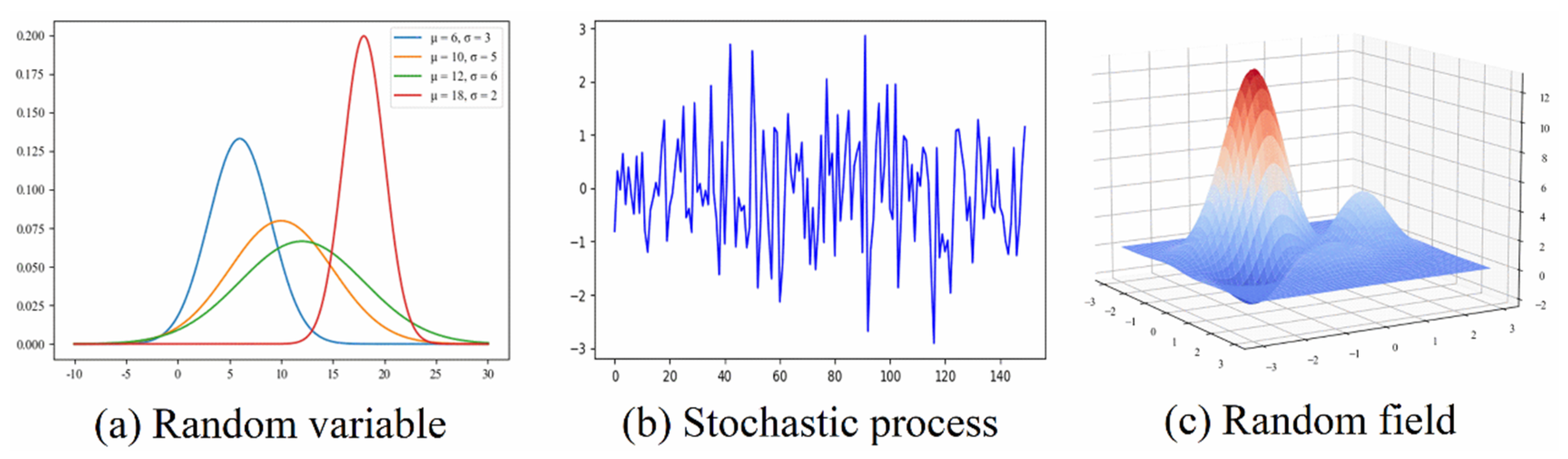
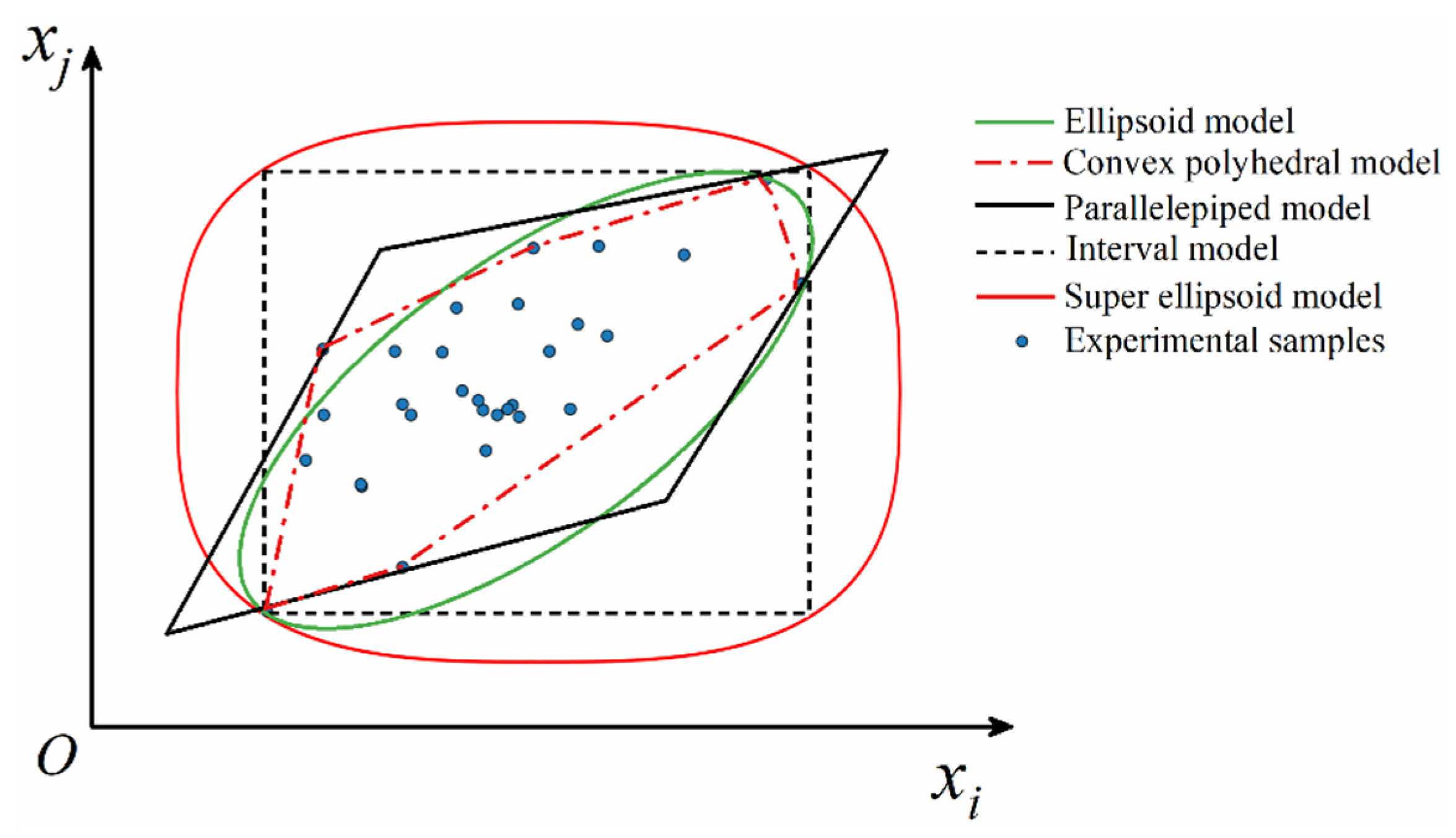
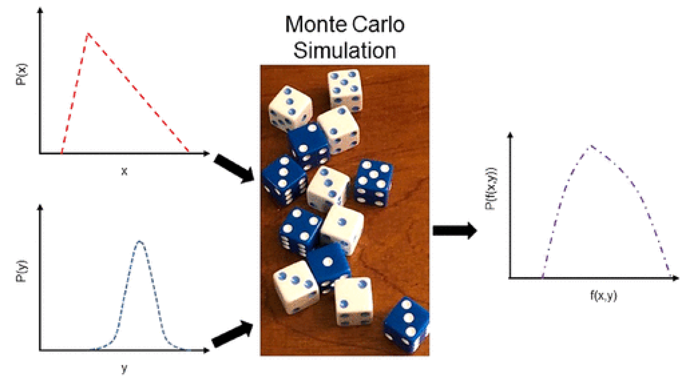
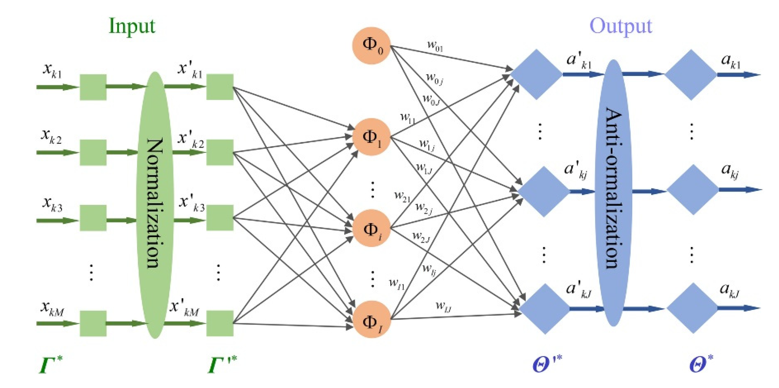
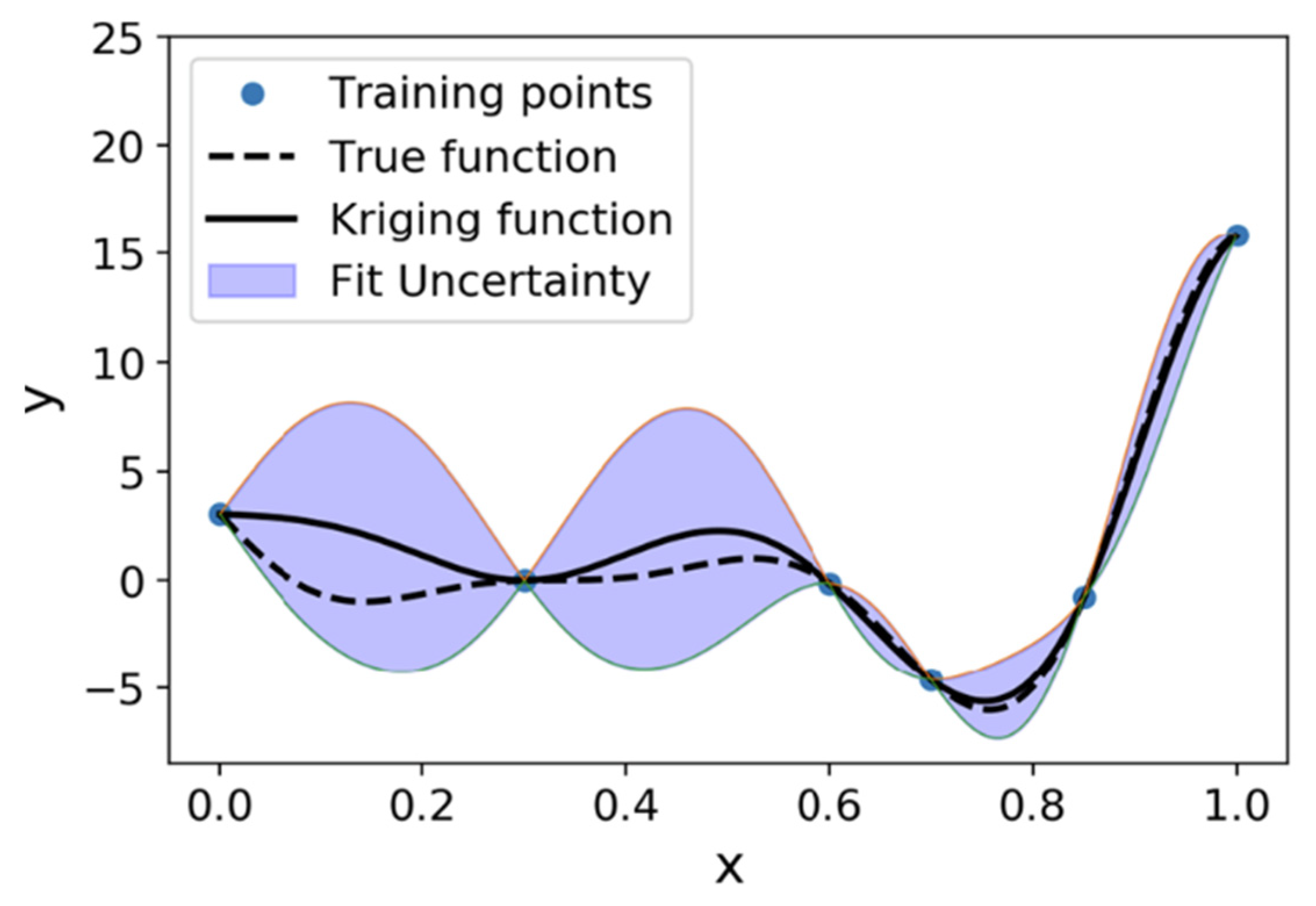
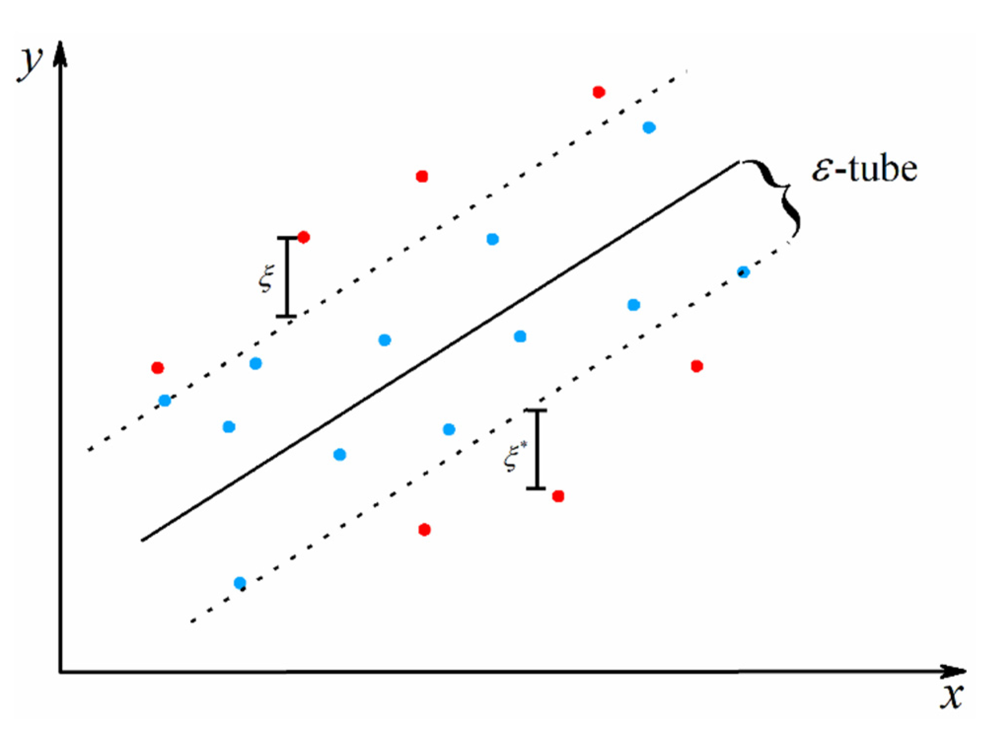
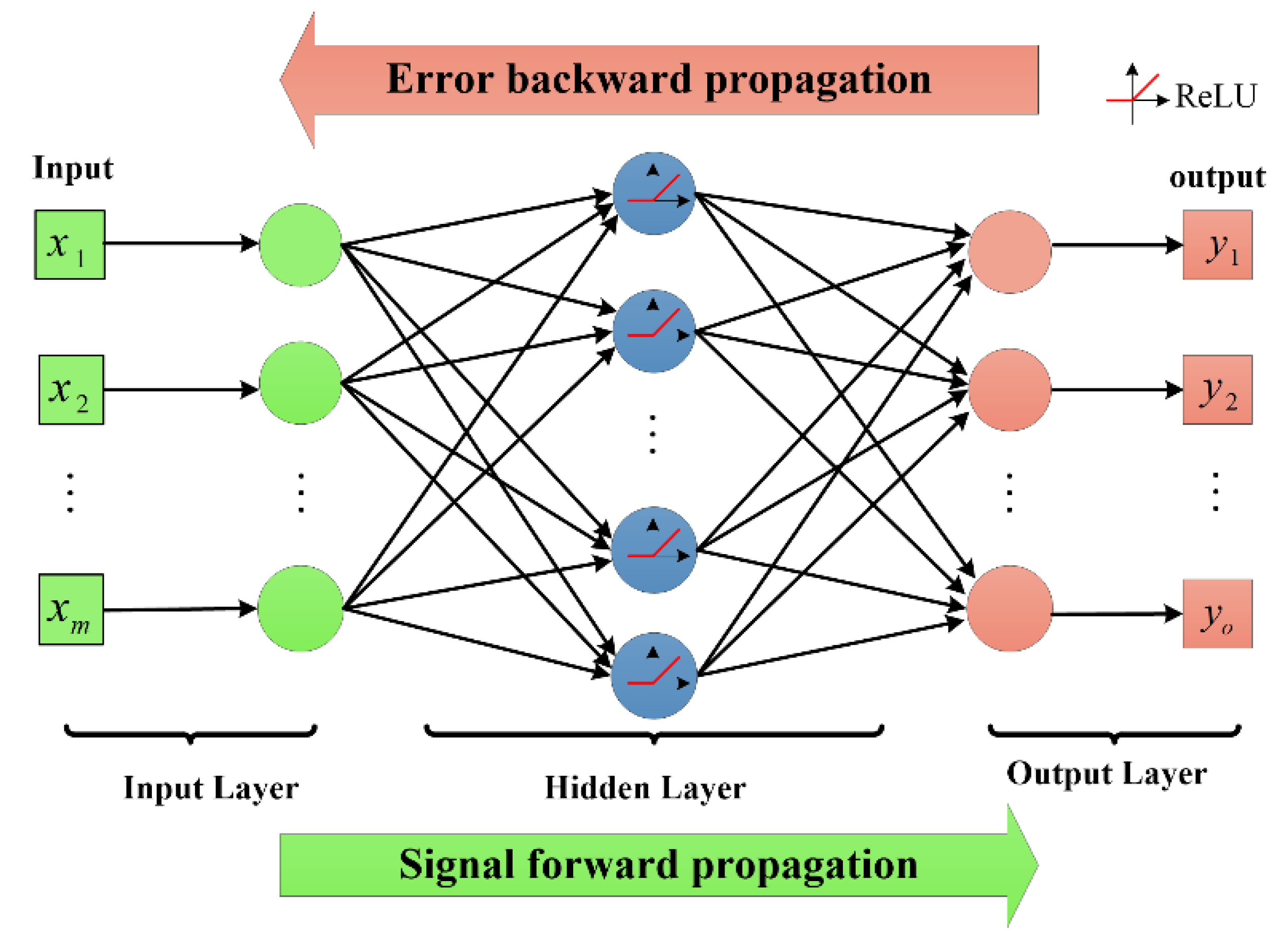
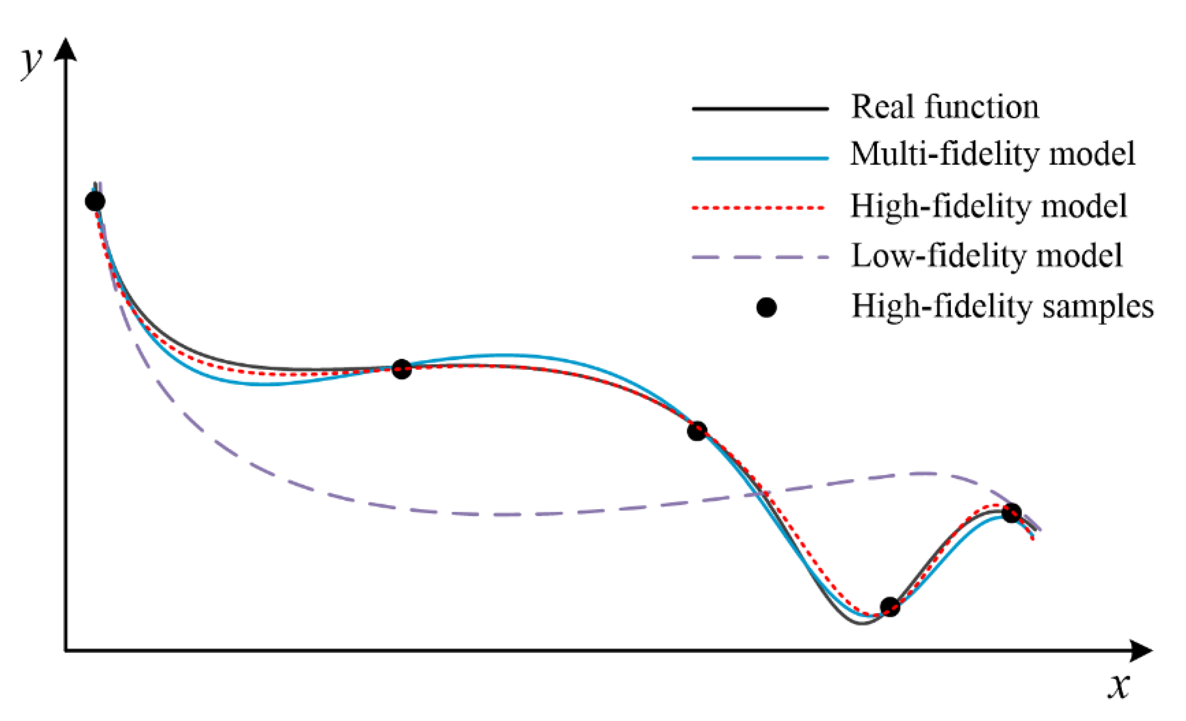
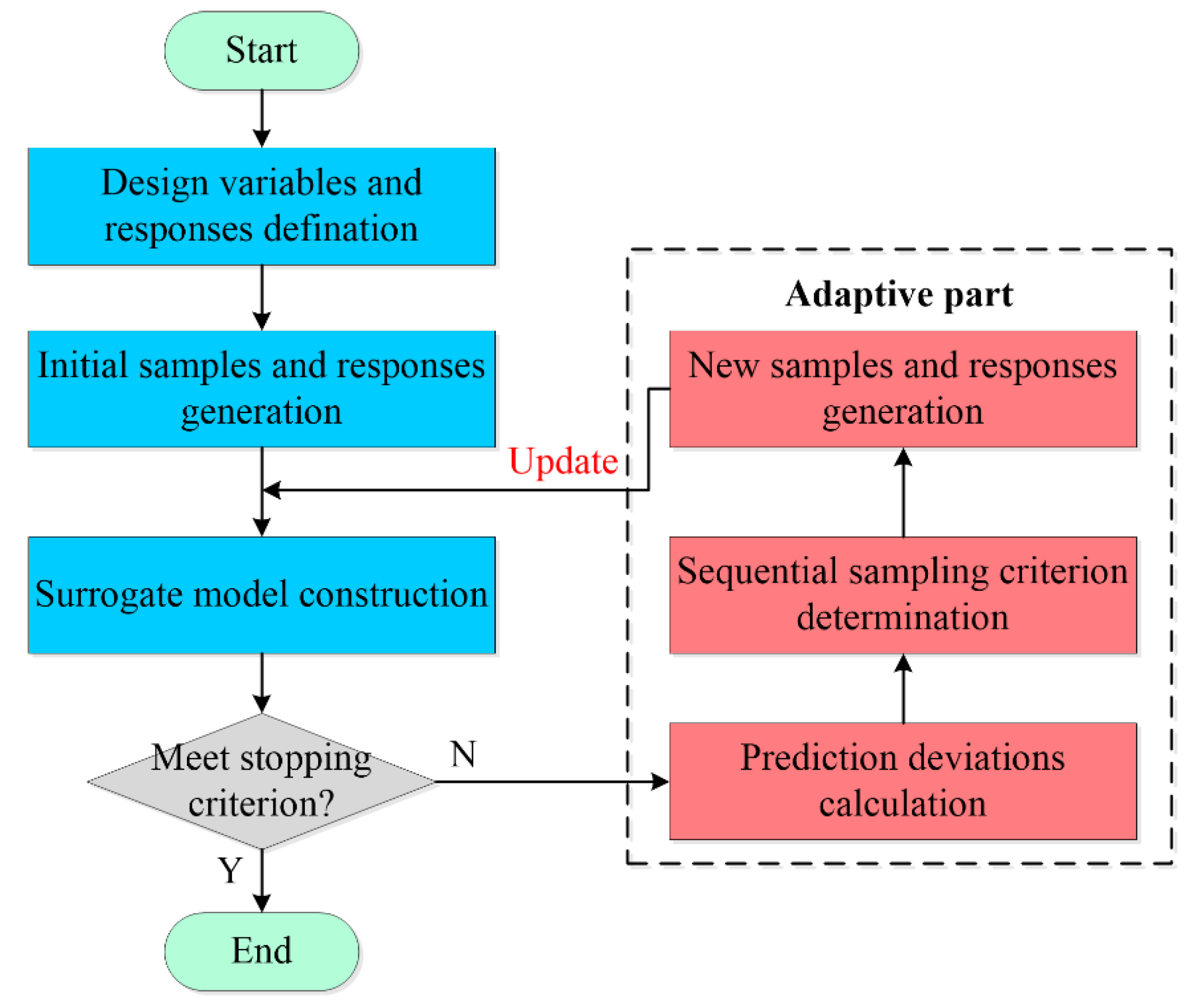
Table 1.
Hybrid strategies for dual-uncertainty modeling in past five years.
| Hybrid Strategy | Uncertainty Involved | Descriptions | Reference Papers |
|---|---|---|---|
| Parallel-type | Probabilistic interval | Mutually independent | [2,76] |
| Probabilistic fuzzy | Mutually independent | [77] | |
| Fuzzy interval | Mutually independent | [6] | |
| Probabilistic convex | Mutually independent | [78] | |
| Fuzzy evidence | Mutually independent | [7,79] | |
| Embedded-type | Probabilistic interval | Distribution parameters of random variables are interval values | [2,80] |
| Probabilistic fuzzy | Distribution parameters of random variables are fuzzy numbers | [40,81] | |
| Fuzzy interval | Interval variables with fuzzy bounds | [75,82] | |
| Fuzzy evidence | Evidence variables with fuzzy focal elements | [83] |
Table 2.
Different types of orthogonal polynomials with distribution.
| Polynomial Type | Distribution | Support |
|---|---|---|
| Hermite | Gaussian | |
| Laguerre | Gamma | |
| Jacobi | Beta | |
| Legendre | Uniform |
Publisher’s Note: MDPI stays neutral with regard to jurisdictional claims in published maps and institutional affiliations. |
© 2022 by the authors. Licensee MDPI, Basel, Switzerland. This article is an open access article distributed under the terms and conditions of the Creative Commons Attribution (CC BY) license (https://creativecommons.org/licenses/by/4.0/).
Share and Cite
MDPI and ACS Style
Wang, C.; Qiang, X.; Xu, M.; Wu, T. Recent Advances in Surrogate Modeling Methods for Uncertainty Quantification and Propagation. Symmetry 2022, 14, 1219. https://doi.org/10.3390/sym14061219
AMA Style
Wang C, Qiang X, Xu M, Wu T. Recent Advances in Surrogate Modeling Methods for Uncertainty Quantification and Propagation. Symmetry. 2022; 14(6):1219. https://doi.org/10.3390/sym14061219
Chicago/Turabian StyleWang, Chong, Xin Qiang, Menghui Xu, and Tao Wu. 2022. "Recent Advances in Surrogate Modeling Methods for Uncertainty Quantification and Propagation" Symmetry 14, no. 6: 1219. https://doi.org/10.3390/sym14061219
Note that from the first issue of 2016, this journal uses article numbers instead of page numbers. See further details here.