
The Numerical Investigation of a Fractional-Order Multi-Dimensional Model of Navier–Stokes Equation via Novel Techniques


1
Department of Basic Sciences, Preparatory Year Deanship King Faisal University, P.O. Box 400, Hofuf, Al-Ahsa 31982, Saudi Arabia
2
Department of Mathematics, Abdul Wali Khan University, Mardan 23200, Pakistan
*
Author to whom correspondence should be addressed.
Symmetry 2022, 14(6), 1102; https://doi.org/10.3390/sym14061102
Submission received: 7 April 2022
/
Revised: 18 May 2022
/
Accepted: 25 May 2022
/
Published: 27 May 2022
(This article belongs to the Topic Engineering Mathematics)
Abstract
:In this study, numerical results of a fractional-order multi-dimensional model of the Navier–Stokes equations will be achieved via adoption of two analytical methods, i.e., the Adomian decomposition transform method and the q-Homotopy analysis transform method. The Caputo–Fabrizio operator will be used to define the fractional derivative. The proposed methods will be implemented to provide the series form results of the given models. The series form results of proposed techniques will be validated with the exact results available in the literature. The proposed techniques will be investigated to be efficient, straightforward, and reliable for application to many other scientific and engineering problems.
1. Introduction
A renowned mathematician, Leibnitz, introduced the concept of fractional derivative in 1695. Fractional calculus is associated with non-integral differential and integral operators. The fractional-order differential operator is a non-local operator, implying that its present and prior states determine a system’s subsequent state. The popularity of fractional calculus increases day by day due to its various implementations in a broad area of non-linear complex systems occurring in viscoelasticity, fluid mechanics, life sciences, mathematical biology, physics, and electrochemistry [1,2,3]. The improvements in fractional differential equations have also received a great deal of attention in recent years [4,5]. There is beauty in symmetry analysis, particularly in the study of partial differential equations, and more specifically those equations coming from the Mathematics of Finance. The secret of nature is symmetry, but most observations in nature do not exhibit symmetry. A profound way to hide symmetry is the phenomenon of spontaneous symmetry-breaking. There are two types of symmetries: finite and infinitesimal. Finite symmetries can be discrete or continuous. Parity and time reversal are discrete symmetries of nature, while space, on the other hand, is a continuous transformation. Mathematicians have forever been fascinated by patterns. Classifications of planar patterns and spatial patterns began seriously in the nineteenth century. Unfortunately, finding an accurate solution to non-linear fractional differential equations has proven quite difficult. Fractional derivatives, for example, can be used to describe non-linear earthquake oscillation, and fractional derivatives can help a fluid dynamic traffic model overcome the inadequacies imposed by the continuum traffic-flow assumption [6,7,8,9,10]. Fractional differential equations have piqued the interest of researchers owing to their precise representation of non-linear processes, particularly in nano-hydrodynamics, where the continuum assumption fails, and the fractional model is the best choice. These discoveries sparked a surge of interest in fractional calculus research across many scientific and technical disciplines [11,12,13].
In 1822, the Navier–Stokes (NS) equation, which governs the motion of the viscous fluid flow, was developed [14,15,16]. The equation is a mixture of the energy equation, the continuity equation, and the momentum equation, and may be thought of as Newton’s second law of motion for fluid substances. This equation may represent a variety of physical phenomena, including liquid flow in pipes, ocean currents, airflow, and blood flow over aircraft wings [17,18,19,20]. Salem and El-Shahed [21] were the first to perform fractional modeling of NS equations in 2005. The authors [21] used the Laplace transform, finite Fourier Sine transform, and finite Hankel transforms to generalize the classical NS equations. Kumar et al. [22] solved a non-linear fractional model of the NS equation analytically by linking the Laplace transform and the homotopy perturbation method. Ganji et al. [23] and Ragab et al. [24] used HAM to solve the non-linear fractional NS equation. For numerical calculation of the fractional NS equation, Maitama [25] and Momani and Birajdar [26] used the Adomian decomposition method. Kumar et al. [27] achieved an approximate result of the time-fractional NS problem by combining the Laplace transform and the Adomian decomposition method, whereas Kumar and Chaurasia [28] solved the same equation by coupling the Laplace transform and finite Hankel transform.
Because most non-linear FDEs do not have precise solutions, numerical approaches are needed to estimate their numerical solution. Modeling the dimensions of equations is vital, but so is the reliability of solution methods. It is self-evident that coupling a technique with a transform [29,30] eliminates time-consuming issues and reduces the amount of CPU time required to investigate numerical solutions to non-linear problems. The q-homotopy analysis transform method (q-HATM) [31,32] is a beautiful combination of the Laplace transform and the q-homotopy analysis method. It has the benefit of including powerful computational approaches for investigating FDEs. By properly selecting, it provides a more effortless technique to regulate the convergence area of the series solution in a broad permitted domain. The series solution’s exact sequence and grid point provide more acceptable results. The efficacy of a key in the convergent zone is demonstrated by h and n-curves. The q-HATM has the advantages of not requiring perturbations, linearization, discretization, or any restrictive assumptions, promising a large convergence region, significantly reducing mathematical calculations, not requiring the computation of complicated polynomials providing a non-local effect, and physical parameters [33,34].
One of the most effective analytical strategies for solving linear and non-linear equations is the Laplace decomposition method [35,36]. The Laplace decomposition method offers benefits over other approximation techniques such as perturbation, since it is free of tiny or big parameters. The Laplace decomposition method does not require any linearization and discretization, unlike other analytical approaches. As a result, the LDM outputs are more realistic and efficient. Approximate solutions to a class of non-linear partial and ordinary differential equations have been obtained using this technique [37,38]. The Klein–Gordon equation [39] and the diffusion-wave equations [40] are two examples. This paper applied the q-homotopy analysis transform method and the Adomian decomposition method combined with a Yang transform Caputo–Fabrizio operator for the first time.
The rest of this article is organized as follows. In Section 2, we present some basic definitions and properties. In Section 3, we give the description of the Adomian decomposition transform method for solving fractional partial differential equations and in Section 4, the existence and uniqueness solution for the Adomian decomposition transform technique. Then, in Section 5, we apply this method to establish a two-dimensional NS equation. In Section 6, we discuss the q-homotopy analysis transform method and graphical discussion. The conclusions are presented at the end of the article.
2. Preliminary Concepts
In this part, we address several key ideas, conceptions, and terminologies related to fractional derivative operators involving index and exponential decay as a kernel, as well as the Yang transform’s specific repercussions.
Definition 2.
Definition 4.
The Yang transform of a range of vital expressions is as follows:
Definition 5.
The inverse Yang transform is defined by
3. The Procedure of Adomian Decomposition Transform Method (ADTM)
In this section, we presented the procedure of ADTM for fractional PDEs [40,43].
with the initial condition
where is the Caputo–Fabrizio derivative of fractional-order , , and , are linear and non-linear terms, respectively, and , are source functions.
ADTM defines the result of infinite series and ,
The non-linear functions defined by Adomian polynomials and are expressed as
The Adomian polynomials can be expressed as
Using the inverse Yang transform on Equation (9),
we expressed the following terms,
the general for , is given by
4. Solution of ADTM
In this section, we apply ADTM coupled with Yang transformation for the Caputo–Fabrizio fractional derivative to solve fractional-order two-dimensional NS equations.
Example 1.
The above equations can be written as
Using the inverse Yang transform, we have
Suppose that the unknown functions and infinite series solution is as follows:
Note that , , and are the Adomian polynomials and the non-linear terms were described. Using some term, Equation (15) can be rewritten in the form
According to Equation (8), the Adomian polynomials can be expressed as
Thus, we can easily achieve the recursive relationship Equation (16)
For
For
For
In same method, the remaining and components of the YDM solution can be obtained seamlessly. Consequently, we describe the series of alternative solutions as
The exact result of Equation (12) at and ,
Example 2.
The above equations can be written as
Applying the inverse Yang transformation, we obtain
Suppose that the unknown functions and infinite series result as follows:
Note that , , and are the Adomian polynomials and the non-linear terms were described. Using some term, Equation (21) can be rewritten in the form
According to Equation (8), the Adomian polynomials can be expressed as
Thus, we can easily achieve the recursive relationship Equation (22)
For
For
For
Using the same method, the remaining and components of the YDM solution can be obtained seamlessly. Consequently, we describe the series of alternative solutions as
The exact result of Equation (18) at and ,
5. The Methodology of q-Homotopy Analysis Transform Method
Consider a non-linear, non-homogeneous fractional partial differential equation [31];
Here, is the Caputo–Fabrizio derivative and R represents the linear and N non-linear terms, respectively. is the source function.
Applying the Yang transform on Equation (24), we get
The non-linear function is
Here, is an unknowns function and are the embedded parameters, . Construct a homotopy as
where is an initial condition and is an auxiliary parameter.
By calculating convergence type to U and intensifying about q by Taylor’s theorem, we get
where
With an appropriated selection of auxiliary linear terms, and H, series (29) convergence at , thereby provides a solution
Applying the inverse transform on Equation (32), we obtain
Here,
and
Lastly, by solving Equation (33), the q-homotopy analysis transform method results elements are readily available.
Example 3.
Define the non-linear operators:
and the Yang operators as
Using the inverse Yang transformation on Equation (40), we have
Using and in Equation (43), we get
as well as others. The remaining components are found in the same manner. The following is the q-HATM result of Equation (36):
For and , results and convergent to exact solutions as :
Example 4.
Consider Equation (36) and take the initial conditions
Define non-linear operators as
and Yang operators as
where
Using the inverse Yang transformation on Equation (48), we get
Using and , we get from Equation (50),
as well as others. The remaining components are found in the same manner. The following is the q-HATM result of Equation (36):
For and , results and convergence to the actual solutions as
6. Results and Discussion
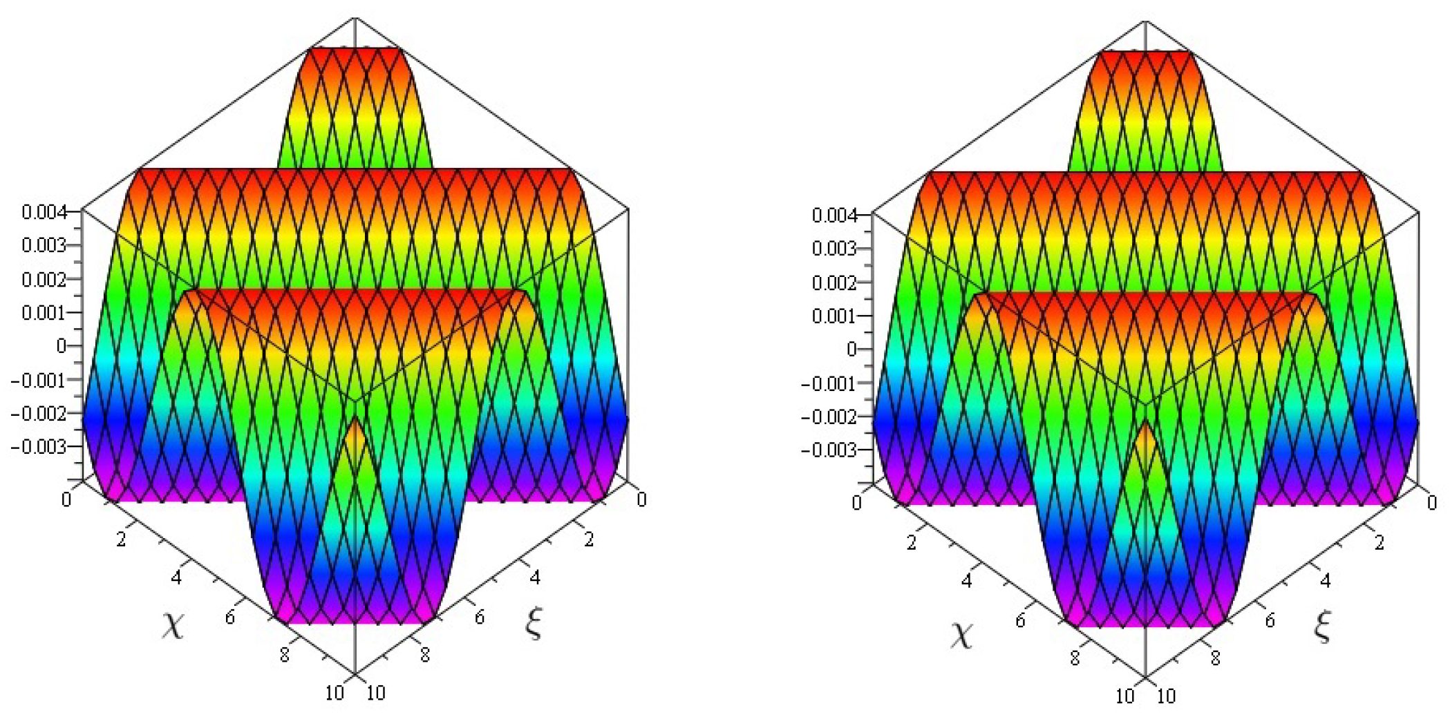
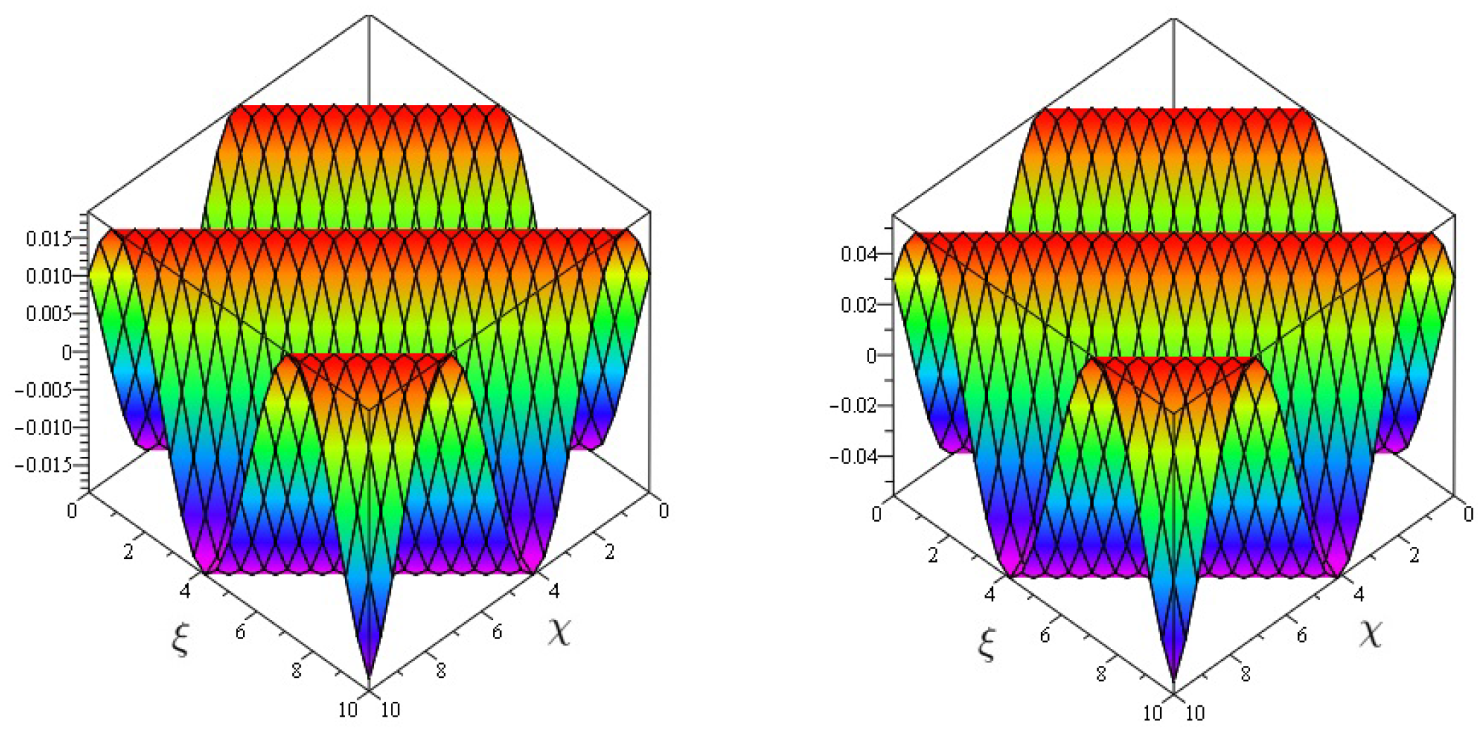
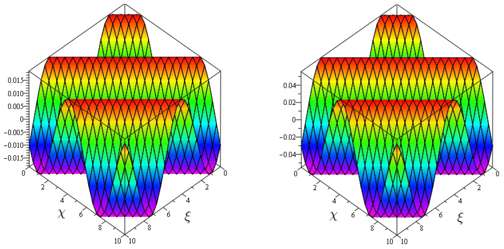
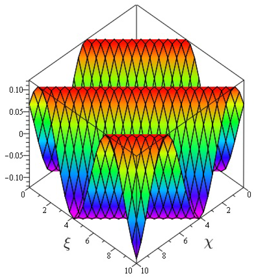
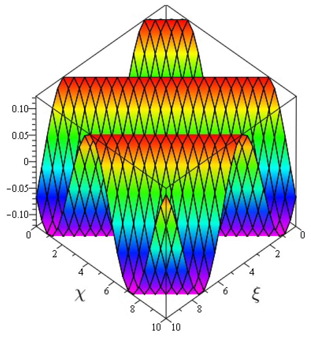
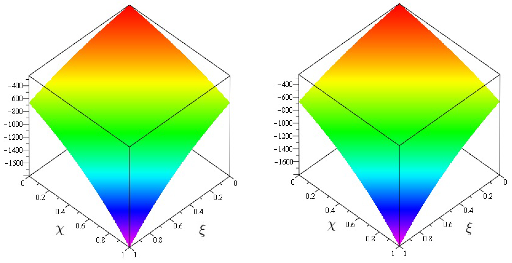
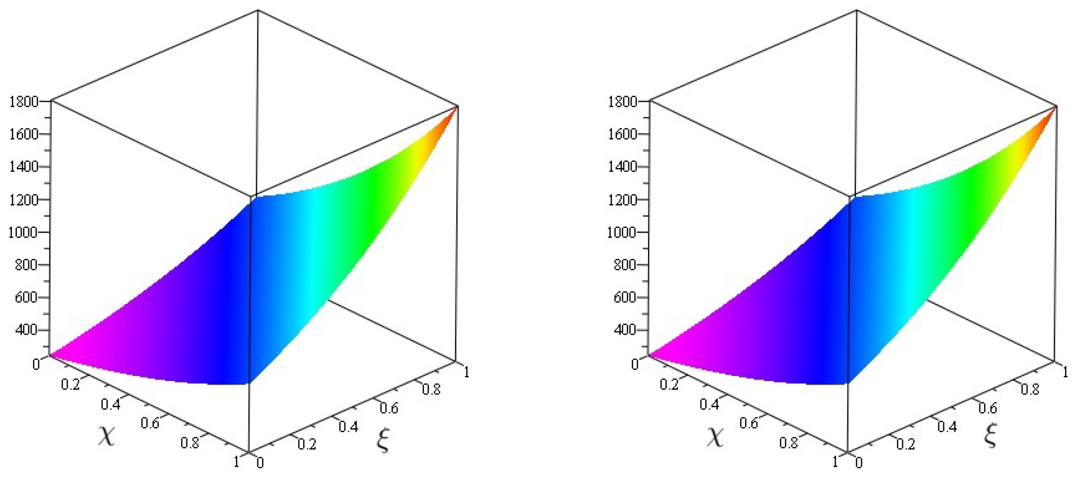
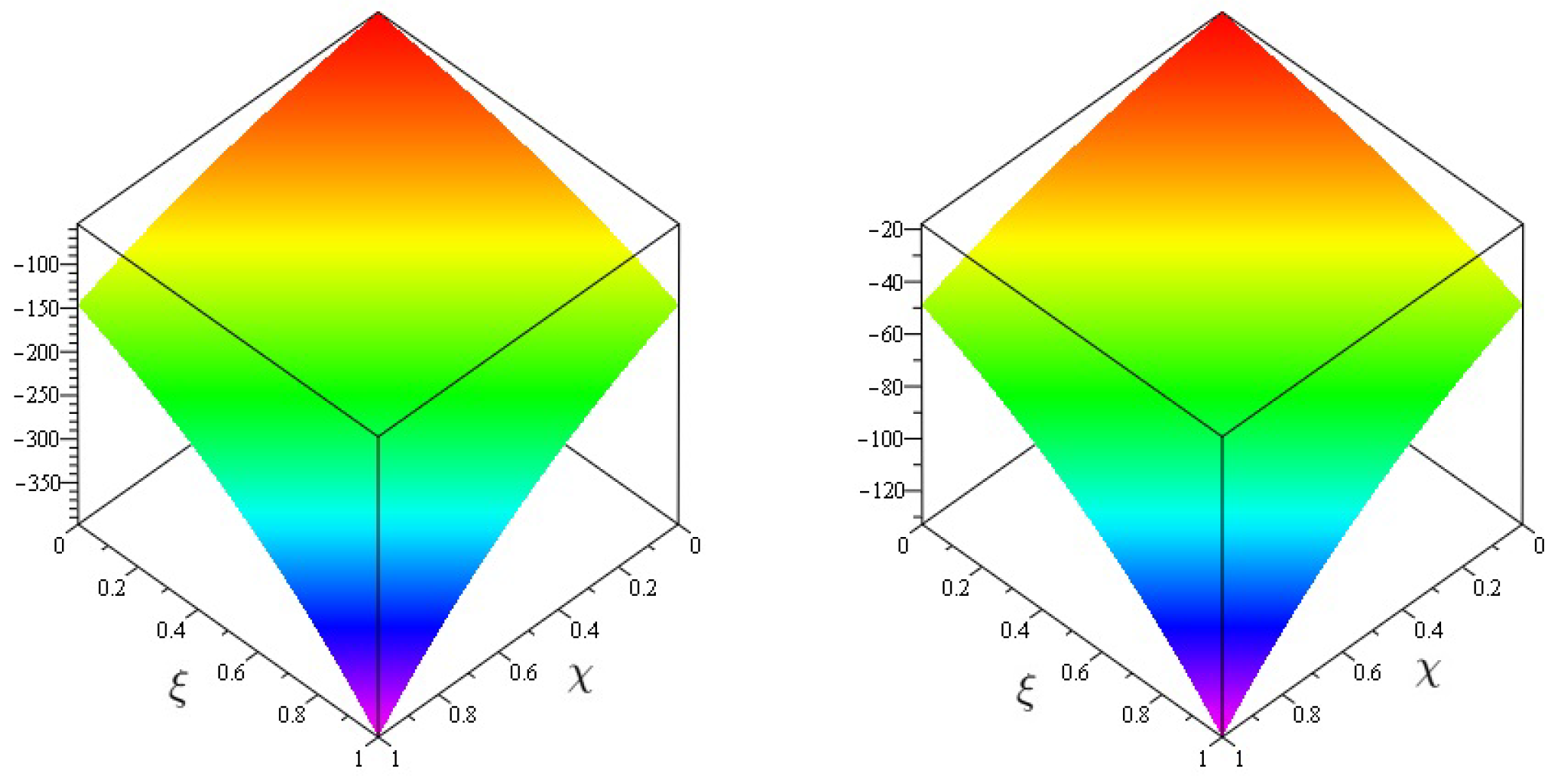
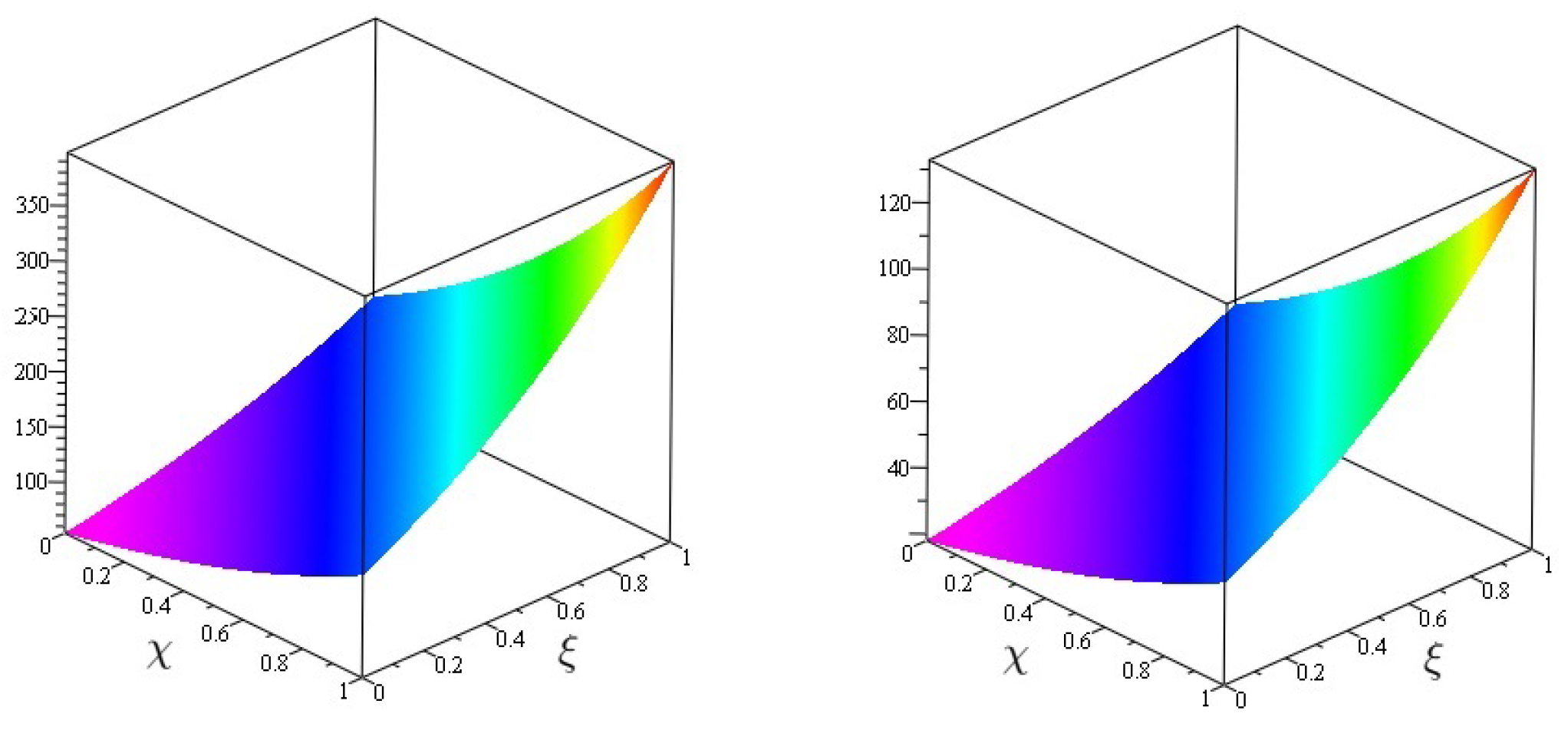
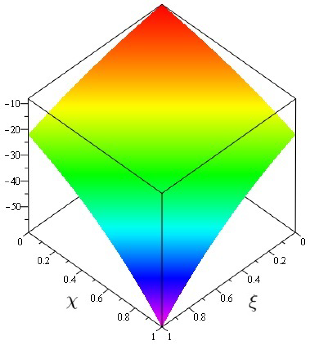
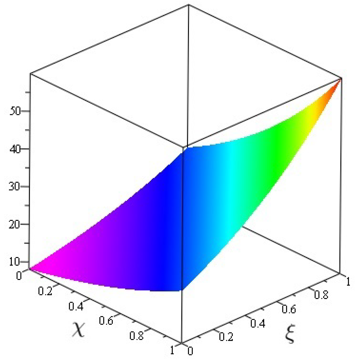
The aim of the this paper is to investigate an analytical solution of fractional-order Navier–Stokes equations, applying efficient analytical methods. The Adomian decomposition transform method and q-homotopy analysis transform method are applied to solve the given examples. The Caputo–Fabrizio definition of fractional derivative is applied to define the fractional derivative. To check the accuracy of the proposed methods, the solution of some illustrative problems are presented. Solutions figures are plotted for both integer and fractional-order problems. In Figure 1, the exact and analytical solution of Example 1 is shown. It is seen that the approximate analytical solution obtained by proposed methods decreases very rapidly with the increases in at the value of . Similarly, in Figure 2, the figures of the exact and analytical solution are represented at . It is observed that the exact, ADTM, and q-HATM solutiosn are in close contact with the exact results of the Examples. In Figure 3, Figure 4, Figure 5 and Figure 6 the ADTM and q-HATM solutions of Example 1 are also calculated at different fractional-order , , . It is confirmed that ADTM and q-HATM solutions are in strong agreement with each other. Similarly, in Figure 7, the exact and analytical solution of Example 2 is shown. In Figure 8, the graph of exact and analytical solution is represented at . It is observed that the exact, ADTM, and q-HATM solutions are in close contact with the exact results of the Examples. Additionally, in Figure 9, Figure 10, Figure 11 and Figure 12 the ADTM and q-HATM solutions of Example 1 are calculated at different fractional-order , , . In Table 1 and Table 2 confirmed that ADTM and q-HATM solutions are in strong agreement with each other. The same convergence phenomena of the fractional-order solutions towards integer-order solutions are observed.
7. Conclusions
This paper evaluates a result of the fractional scheme of Navier–Stokes equations calculating numerical results utilizing the proposed q-homotopy analysis transform method and the Yang decomposition method. In a rapid convergence series, the solution is attained. The efficacy and effectiveness of the method are demonstrated by the test samples presented. The suggested approach incorporates a parameter ℏ that controls the convergence zone of the series solution. Because the q-homotopy analysis transform method and the Yang decomposition approach do not require minor perturbations, linearization, or discretization, computation times are greatly reduced. The q-homotopy analysis transform method and Yang decomposition method are competent tools for obtaining mathematical results of system non-linear fractional partial differential equations when compared to other methodologies.
Author Contributions
Formal analysis, S.M.; Methodology, R.S.; Project administration, S.N.; Software, R.S.; Supervision, S.M.; Validation, S.N; Writing—original draft, R.S.; Writing—review & editing, S.M. All authors have equal contribution. All authors have read and agreed to the published version of the manuscript.
Funding
This work was supported through the annual funding track by the Deanship of Scientific Research, Vice Presidency of Graduate Studies and Scientific Research King Faisal University Saudi Arabia (project No. AN000377).
Institutional Review Board Statement
Not applicable.
Informed Consent Statement
Not applicable.
Data Availability Statement
The numerical data used to support the findings of this study are included within the article.
Acknowledgments
This work was supported through the annual funding track by the Deanship of Scientific Research, Vice Presidency of Graduate Studies and Scientific Research King Faisal University Saudi Arabia (project No. AN000377).
Conflicts of Interest
The authors declare no conflict of interest.
References
- Caputo, M.; Fabrizio, M. A new definition of fractional derivative without singular kernel. Progr. Fract. Differ. Appl. 2015, 1, 1–13. [Google Scholar]
- Sheikh, N.A.; Ali, F.; Khan, I.; Saqib, M. A modern approach of Caputo-Fabrizio time-fractional derivative to MHD free convection flow of generalized second-grade fluid in a porous medium. Neural Comput. Appl. 2018, 30, 1865–1875. [Google Scholar] [CrossRef]
- Atangana, A.; Alqahtani, R.T. Numerical approximation of the space-time Caputo-Fabrizio fractional derivative and application to groundwater pollution equation. Adv. Differ. Equ. 2016, 2016, 156. [Google Scholar] [CrossRef] [Green Version]
- Aljahdaly, N.; Akgül, A.; Shah, R.; Mahariq, I.; Kafle, J. A Comparative Analysis of the Fractional-Order Coupled Korteweg–De Vries Equations with the Mittag–Leffler Law. J. Math. 2022, 2022, 1–30. [Google Scholar] [CrossRef]
- Shamshuddin, M.D.; Mishra, S.R.; Beg, O.A.; Kadir, A. Numerical study of heat transfer and viscous flow in a dual rotating extendable disk system with a non-Fourier heat flux model. Heat Transf. Asian Res. 2019, 48, 435–459. [Google Scholar] [CrossRef]
- Gao, X.Y.; Guo, Y.J.; Shan, W.R. Bilinear forms through the binary Bell polynomials, N solitons and Backlund transformations of the Boussinesq-Burgers system for the shallow water waves in a lake or near an ocean beach. Commun. Theor. Phys. 2020, 72, 095002. [Google Scholar] [CrossRef]
- Gao, X.Y.; Guo, Y.J.; Shan, W.R. Optical waves/modes in a multicomponent inhomogeneous optical fiber via a three-coupled variable-coefficient nonlinear Schrodinger system. Appl. Math. Lett. 2021, 120, 107161. [Google Scholar] [CrossRef]
- Gao, X.Y.; Guo, Y.J.; Shan, W.R. Symbolic computation on a (2+1)-dimensional generalized variable-coefficient Boiti-Leon-Pempinelli system for the water waves. Chaos Solitons Fractals 2021, 150, 111066. [Google Scholar] [CrossRef]
- Gao, X.Y.; Guo, Y.J.; Shan, W.R. Looking at an open sea via a generalized (2+1)-dimensional dispersive long-wave system for the shallow water: Scaling transformations, hetero-Backlund transformations, bilinear forms and N solitons. Eur. Phys. J. Plus 2021, 136, 1–9. [Google Scholar] [CrossRef]
- Gao, X.Y.; Guo, Y.J.; Shan, W.R.; Yin, H.M.; Du, X.X.; Yang, D.Y. Certain electromagnetic waves in a ferromagnetic film. Commun. Nonlinear Sci. Numer. Simul. 2022, 105, 106066. [Google Scholar] [CrossRef]
- Saad, K.M.; Atangana, A.; Baleanu, D. New fractional derivatives with non-singular kernel applied to the Burgers equation. Chaos Interdiscip. J. Nonlinear Sci. 2018, 28, 063109. [Google Scholar] [CrossRef]
- Nonlaopon, K.; Naeem, M.; Zidan, A.; Shah, R.; Alsanad, A.; Gumaei, A. Numerical Investigation of the Time-Fractional Whitham–Broer–Kaup Equation Involving without Singular Kernel Operators. Complexity 2021, 2021, 1–21. [Google Scholar] [CrossRef]
- Baleanu, D.; Machado, J.A.T.; Luo, A.C. Fractional Dynamics and Control; Springer: New York, NY, USA, 2012. [Google Scholar]
- Poincare, H. Memoires et observations. Sur l’equilibre d’une masse fluide animee d’un mouvement de rotation. Bull. Astron. Ser. I 1885, 2, 109–118. [Google Scholar] [CrossRef]
- Adomian, G. Analytical solution of Navier-Stokes flow of a viscous compressible fluid. Found. Phys. Lett. 1995, 8, 389–400. [Google Scholar] [CrossRef]
- Krasnoschok, M.; Pata, V.; Siryk, S.V.; Vasylyeva, N. A subdiffusive Navier-Stokes-Voigt system. Phys. D Nonlinear Phenom. 2020, 409, 132503. [Google Scholar] [CrossRef]
- Wang, Y.; Zhao, Z.; Li, C.; Chen, Y.Q. Adomian’s method applied to Navier-Stokes equation with a fractional order. In Proceedings of the ASME 2009 IDETC/CIE, San Diego, CA, USA, 30 August–2 September 2009; pp. 1047–1054. [Google Scholar]
- Yu, Q.; Song, J.; Liu, F.; Anh, V.; Turner, I. An approximate solution for the Rayleigh-Stokes problem for a heated generalized second grade fluid with fractional derivative model using the Adomian decomposition method. J. Algorithms Comput. Technol. 2009, 3, 553–571. [Google Scholar] [CrossRef]
- Krasnoschok, M.; Pata, V.; Siryk, S.V.; Vasylyeva, N. Equivalent definitions of Caputo derivatives and applications to subdiffusion equations. Dyn. PDE 2020, 17, 383–402. [Google Scholar] [CrossRef]
- Bazhlekova, E.; Jin, B.; Lazarov, R.; Zhou, Z. An analysis of the Rayleigh-Stokes problem for a generalized second-grade fluid. Numer. Math. 2015, 131, 1–31. [Google Scholar] [CrossRef] [PubMed] [Green Version]
- El-Shahed, M.; Salem, A. On the generalized Navier-Stokes equations. Appl. Math. Comput. 2004, 156, 287–293. [Google Scholar] [CrossRef]
- Kumar, D.; Singh, J.; Kumar, S. A fractional model of Navier-Stokes equation arising in unsteady flow of a viscous fluid. J. Assoc. Arab. Univ. Basic Appl. Sci. 2015, 17, 14–19. [Google Scholar] [CrossRef] [Green Version]
- Ganji, Z.Z.; Ganji, D.D.; Ganji, A.D.; Rostamian, M. Analytical solution of time-fractional Navier-Stokes equation in polar coordinate by homotopy perturbation method. Numer. Methods Partial. Differ. Equ. Int. J. 2010, 26, 117–124. [Google Scholar] [CrossRef]
- Ragab, A.A.; Hemida, K.M.; Mohamed, M.S.; Abd El Salam, M.A. Solution of time-fractional Navier-Stokes equation by using homotopy analysis method. Gen. Math. Notes 2012, 13, 13–21. [Google Scholar]
- Maitama, S. Analytical solution of time-fractional Navier-Stokes equation by natural homotopy perturbation method. Prog. Fract. Differ. Appl. 2018, 4, 123–131. [Google Scholar] [CrossRef]
- Birajdar, G.A. Numerical solution of time fractional Navier-Stokes equation by discrete Adomian decomposition method. Nonlinear Eng. 2014, 3, 21–26. [Google Scholar] [CrossRef]
- Kumar, S.; Kumar, D.; Abbasbandy, S.; Rashidi, M.M. Analytical solution of fractional Navier-Stokes equation by using modified Laplace decomposition method. Ain Shams Eng. J. 2014, 5, 569–574. [Google Scholar] [CrossRef] [Green Version]
- Chaurasia, V.B.L.; Kumar, D. Solution of the time-fractional Navier-Stokes equation. Gen. Math. Notes 2011, 4, 49–59. [Google Scholar]
- Prakash, A.; GAlaoui, M.; Fayyaz, R.; Khan, A.; Shah, R.; Abdo, M. Analytical Investigation of Noyes–Field Model for Time-Fractional Belousov–Zhabotinsky Reaction. Complexity 2021, 2021, 1–21. [Google Scholar]
- El-Tawil, M.A.; Huseen, S.N. On convergence of the q-homotopy analysis method. Int. J. Contemp. Math. Sci. 2013, 8, 481–497. [Google Scholar] [CrossRef]
- Prakash, A.; Veeresha, P.; Prakasha, D.G.; Goyal, M. A new efficient technique for solving fractional coupled Navier-Stokes equations using q-homotopy analysis transform method. Pramana 2019, 93, 1–10. [Google Scholar] [CrossRef]
- Arafa, A.A.; Hagag, A.M.S. Q-homotopy analysis transform method applied to fractional Kundu-Eckhaus equation and fractional massive Thirring model arising in quantum field theory. Asian-Eur. J. Math. 2019, 12, 1950045. [Google Scholar] [CrossRef]
- Jena, R.M.; Chakraverty, S. Q-Homotopy Analysis Aboodh Transform Method based solution of proportional delay time-fractional partial differential equations. J. Interdiscip. Math. 2019, 22, 931–950. [Google Scholar] [CrossRef]
- Iqbal, N.; Akgül, A.; Shah, R.; Bariq, A.; Mossa Al-Sawalha, M.; Ali, A. On Solutions of Fractional-Order Gas Dynamics Equation by Effective Techniques. J. Funct. Spaces 2022, 2022, 1–14. [Google Scholar] [CrossRef]
- Khuri, S.A. A Laplace decomposition algorithm applied to a class of nonlinear differential equations. J. Appl. Math. 2001, 1, 141–155. [Google Scholar] [CrossRef]
- Khuri, S.A. A new approach to Bratus problem. Appl. Math. Comput. 2004, 147, 131–136. [Google Scholar]
- Mohamed, M.A.; Torky, M.S. Numerical solution of nonlinear system of partial differential equations by the Laplace decomposition method and the Pade approximation. Am. J. Comput. Math. 2013, 3, 175. [Google Scholar] [CrossRef] [Green Version]
- Ghazi, F.F.; Tawfiq, L.N.M. Coupled Laplace-decomposition method for solving Klein-Gordon equation. Int. J. Mod. Math. Sci. 2020, 18, 31–41. [Google Scholar]
- Hosseinzadeh, H.; Jafari, H.; Roohani, M. Application of Laplace decomposition method for solving Klein-Gordon equation. World Appl. Sci. J. 2010, 8, 809–813. [Google Scholar]
- Khan, H.; Farooq, U.; Shah, R.; Baleanu, D.; Kumam, P.; Arif, M. Analytical Solutions of (2+Time Fractional Order) Dimensional Physical Models, Using Modified Decomposition Method. Appl. Sci. 2019, 10, 122. [Google Scholar] [CrossRef] [Green Version]
- Yang, X.J. A new integral transform method for solving steady heat-transfer problem. Therm. Sci. 2016, 20 (Suppl. 3), 639–642. [Google Scholar] [CrossRef] [Green Version]
- Caputo, M.; Fabrizio, M. On the singular kernels for fractional derivatives. some applications to partial differential equations. Progr. Fract. Differ. Appl. 2021, 7, 1–4. [Google Scholar]
- Shah, R.; Khan, H.; Baleanu, D. Fractional Whitham–Broer–Kaup Equations within Modified Analytical Approaches. Axioms 2019, 8, 125. [Google Scholar] [CrossRef] [Green Version]
Figure 1.
The figure of actual and q-HATM/ADTM solution of at and of example 1 and 3.

Figure 2.
The figure of actual and q-HATM/ADTM solutions of at and of example 1 and 3.

Figure 3.
The various fractional-order solution of at and of example 1 and 3.

Figure 4.
The various fractional-order solution of at and of example 1 and 3.

Figure 5.
The figure of analytic solution of at of example 1 and 3.

Figure 6.
The figure of analytic solution of at of example 1 and 3.

Figure 7.
The figure of actual and q-HATM/ADTM solution of at and of example 2 and 4.

Figure 8.
The figure of actual and q-HATM/ADTM solution of at and of example 2 and 4.

Figure 9.
The various fractional-order solution of at and of example 2 and 4.

Figure 10.
The various fractional-order solution of at and of example 2 and 4.

Figure 11.
The figure of analytical result of at of example 2 and 4.

Figure 12.
The figure of analytical result of at of example 2 and 4.


Table 1.
Comparative study between LDM [27], and for the numerical result of Example 1.
Table 1.
Comparative study between LDM [27], and for the numerical result of Example 1.
| 0.1 | 4.3210 | 4.2464 | 4.2464 | |
| 0.2 | 5.890 | 4.5486 | 4.5486 | |
| 0.1 | 0.3 | 2.7301 | 2.3578 | 2.3578 |
| 0.4 | 5.9700 | 6.3267 | 6.3267 | |
| 0.5 | 2.9771 | 3.2436 | 3.2436 | |
| 0.1 | 2.4400 | 4.7421 | 4.7421 | |
| 0.2 | 8.3100 | 3.1235 | 3.1235 | |
| 0.2 | 0.3 | 2.8500 | 4.5682 | 4.5682 |
| 0.4 | 9.7940 | 3.5223 | 3.5223 | |
| 0.5 | 3.2012 | 2.9315 | 2.9315 | |
| 0.1 | 2.2981 | 3.2245 | 3.2245 | |
| 0.2 | 5.4602 | 4.2659 | 4.2659 | |
| 0.3 | 0.3 | 2.5432 | 1.5348 | 1.5348 |
| 0.4 | 6.4229 | 8.2374 | 8.2374 | |
| 0.5 | 2.8364 | 4.1975 | 4.1975 | |
| 0.1 | 5.5428 | 2.1351 | 2.1351 | |
| 0.2 | 2.4133 | 2.6276 | 2.6276 | |
| 0.4 | 0.3 | 6.3743 | 2.2334 | 2.2334 |
| 0.4 | 2.9070 | 1.2035 | 1.2035 | |
| 0.5 | 6.9763 | 2.2145 | 2.2145 | |
| 0.1 | 2.2529 | 2.3223 | 2.3223 | |
| 0.2 | 4.9868 | 3.2721 | 3.2721 | |
| 0.5 | 0.3 | 4.1932 | 3.0767 | 3.0767 |
| 0.4 | 5.5568 | 2.3742 | 2.3742 | |
| 0.5 | 2.4350 | 1.3223 | 1.3223 |
Table 2.
Comparative study between LDM [27], and for the numerical result of Example 1.
Table 2.
Comparative study between LDM [27], and for the numerical result of Example 1.
| 0.1 | 9.0202 | 1.3770 | 8.6253 | |
| 0.2 | 5.4060 | 4.8036 | 3.1054 | |
| 0.1 | 0.3 | 2.7960 | 1.6734 | 1.1992 |
| 0.4 | 6.5902 | 5.8013 | 5.5827 | |
| 0.5 | 3.9762 | 1.9773 | 3.6150 | |
| 0.1 | 3.3610 | 2.3548 | 2.8894 | |
| 0.2 | 9.1810 | 8.2143 | 1.0171 | |
| 0.2 | 0.3 | 1.9482 | 2.8611 | 3.6538 |
| 0.4 | 9.8750 | 9.2053 | 1.4010 | |
| 0.5 | 4.2127 | 3.3727 | 6.3855 | |
| 0.1 | 2.3872 | 1.2779 | 2.3189 | |
| 0.2 | 5.3523 | 4.4573 | 8.1227 | |
| 0.3 | 0.3 | 2.5565 | 1.5522 | 2.8704 |
| 0.4 | 6.3787 | 5.3749 | 1.0445 | |
| 0.5 | 2.8365 | 1.8244 | 4.1512 | |
| 0.1 | 5.2272 | 4.3423 | 1.0363 | |
| 0.2 | 2.6215 | 1.5145 | 3.6229 | |
| 0.4 | 0.3 | 6.3642 | 5.2723 | 1.2717 |
| 0.4 | 2.9203 | 1.8244 | 4.5250 | |
| 0.5 | 6.9958 | 6.1751 | 1.6814 | |
| 0.1 | 2.2532 | 1.1434 | 3.3630 | |
| 0.2 | 4.8935 | 3.9879 | 1.1745 | |
| 0.5 | 0.3 | 2.4921 | 1.3880 | 4.1074 |
| 0.4 | 5.8486 | 4.7977 | 1.4434 | |
| 0.5 | 1.6542 | 1.6182 | 5.1527 |
Publisher’s Note: MDPI stays neutral with regard to jurisdictional claims in published maps and institutional affiliations. |
© 2022 by the authors. Licensee MDPI, Basel, Switzerland. This article is an open access article distributed under the terms and conditions of the Creative Commons Attribution (CC BY) license (https://creativecommons.org/licenses/by/4.0/).
Share and Cite
MDPI and ACS Style
Mukhtar, S.; Shah, R.; Noor, S. The Numerical Investigation of a Fractional-Order Multi-Dimensional Model of Navier–Stokes Equation via Novel Techniques. Symmetry 2022, 14, 1102. https://doi.org/10.3390/sym14061102
AMA Style
Mukhtar S, Shah R, Noor S. The Numerical Investigation of a Fractional-Order Multi-Dimensional Model of Navier–Stokes Equation via Novel Techniques. Symmetry. 2022; 14(6):1102. https://doi.org/10.3390/sym14061102
Chicago/Turabian StyleMukhtar, Safyan, Rasool Shah, and Saima Noor. 2022. "The Numerical Investigation of a Fractional-Order Multi-Dimensional Model of Navier–Stokes Equation via Novel Techniques" Symmetry 14, no. 6: 1102. https://doi.org/10.3390/sym14061102
Note that from the first issue of 2016, this journal uses article numbers instead of page numbers. See further details here.