Design of a New Dimension-Changeable Hyperchaotic Model Based on Discrete Memristor

Abstract

The application of a memristor in chaotic circuits is increasingly becoming a popular research topic. The influence of a memristor on the dynamics of chaotic systems is worthy of further exploration. In this paper, a multi-dimensional closed-loop coupling model based on a Logistic map and Sine map (CLS) is proposed. The new chaotic model is constructed by cascade operation in which the output of the Logistic map is used as the input of the Sine map. Additionally, the one-dimensional map is extended to any dimension through the coupling modulation. In order to further increase the complexity and stability of CLS, the discrete memristor model is introduced to construct a discrete memristor-based coupling model with a Logistic map and a Sine map (MCLS). By analyzing the Lyapunov exponents, bifurcation diagram, complexity, and the 0–1 test result, the comparison result between CLS and MCLS is obtained. The dynamics performance analysis shows that the Lyapunov exponents and bifurcation diagrams present symmetrical distribution with variations of some parameters. The MCLS has parameters whose values can be set in a wider range and can generate more complex and more stable chaotic sequences. It proves that the proposed discrete memristor-based closed-loop coupling model can produce any higher dimension hyperchaotic system and the discrete memristor model can effectively improve the performance of discrete chaotic map and make this hyperchaotic system more stable.

1. Introduction

Among the data protection schemes, extensive attention has been paid to the encryption scheme design based on the chaotic system because of its good security effect [1,2]. Through the chaotic system, it can use the fixed calculation rules to produce a sequence with complex numerical variations and random characteristics. After a reasonable design, it can meet the current needs of information security encryption [3,4]. Therefore, it is extremely essential to design chaotic systems.

The improvement of existing chaotic systems is mostly based on some classical chaos, such as the Chen system [5], Logistic map [6], Sine map [7], and so on. M. Alawida et al. [8] designed a one-dimensional model to expand the chaotic effect of classical chaotic maps. Z. Hua et al. [9] proposed a model based on cosine transformation to improve the 1D chaotic system. A hybrid 2D chaotic map based on a sine-cosine cross-chaotic map was designed by N. Khalil et al. [10]. There are also many studies on the improved design of high-dimensional chaotic systems. C. Wu et al. [11] designed a chaotic system using the coupling and modulation method. Q. Wu [12] used the cascade operation to design a chaotic model. Additionally, deep learning was also applied for the improvement of the chaotic system by Z. P. Zhao et al. [13]. X. Yong et al. [14] applied fractional-order theory to the Lorenz system to improve the state of the system. X. Xu et al. [15] extended and enhanced multi-scroll chaotic system using the Julia fractal.

A memristor is an electronic component that controls electric charge through the magnetic flux. The concept was first proposed by L. Chua [16] in 1971, and only in 2008 did D. B. Strukov et al. [17] realize it through experiments. Then research based on the hardware implementation for different forms of memristors has been conducted [18,19]. It is still being explored in recent years [20,21,22]. Nowadays, memristors are applied in several fields. In artificial intelligence, algorithms with memristors can effectively improve learning ability [23]. A memristor is also applied in the neural network for its switch behavior [24]. Adding a memristor in the design of the chaotic circuit can also make the chaotic circuit show more complex dynamic characteristics. A memristor-based Lü system that can generate multi-scroll and a memristor-based novel 3D chaotic system combined with the Julia fractal was designed by Yan et al. [25,26]. The design of discrete memristors and their application for chaotic systems is discussed. Peng et al. [27] designed a discrete memristor to apply to the chaotic system to improve its chaotic behavior. Fu et al. [28] designed a discrete-memristor-based Lorenz system and realize its Simulink modeling. He et al. [29] designed a discrete fracmemristor in which the amount of charge is determined by a fractional-order discrete system. Bao et al. [30] present a new second-order discrete map model deriving from a simple sampling switch-based memristor-capacitor circuit. The research above shows that discrete memristor models can present complex dynamic performances of chaotic systems. Additionally, Li et al. [31] used the discrete memristor model to design two discrete memristors with cosine with amplitude memristance and built the Simulink models to verify that they meet the definition of the memristor.

Discrete chaotic systems are easy to implement in hardware because they have a simple structure and do not need to solve differential equations. Although a discrete chaotic system has an excellent performance in the application of image encryption, the insufficient complexity, the limited number, and the range of variable parameters could lead to the vulnerability of encrypted information to resist attacks. Therefore, designing a numerical sequence that can produce a wider distribution range and stronger randomness is the premise to improve the security of encryption. For this motivation, a novel discrete dimension-changeable hyperchaotic system is combined with a memristor to explore the effectiveness of improving the complexity of the system. To enhance the randomness of the chaotic model and the flexibility of parameter variation, a chaotic model with large parameter ranges and flexible dimension change is proposed. The chaotic system can expand the existing one-dimensional chaotic maps to any dimension. Additionally, to deepen the application of memristors in the design of chaotic systems, a discrete memristor-based model is constructed to explore the influence of the memristor on the dynamics performance of the proposed chaotic system. In the following work, the simulation is conducted to show the effectiveness of the discrete memristor in enhancing the randomness and chaos stability of the proposed discrete hyperchaotic system.

The following parts of the paper are organized as follows. In Section 2, the discrete memristor model is introduced. In Section 3, the discrete hyperchaotic model with variable dimensions based on cascade and coupling is proposed. The discrete memristor is added in the proposed hyperchaotic model. In Section 4, the chaotic performance of the hyperchaotic system before and after adding discrete memristor is compared and analyzed. The conclusion of the paper is given in Section 5.

2. Construction of Discrete Memristor Model for Improving Chaotic System

According to the definition given in 1971, a memristor can be obtained by the following formula [16]

$$M\left(q\right)=\frac{d\phi }{dq}.$$

(1)

According to the basic circuit knowledge, we can get the continuous-time memristor model

$$\left\{\begin{array}{c}M\left(q\left(t\right)\right)=\frac{d\phi }{dq}\hfill \\ ki\left(t\right)=\frac{dq}{dt}\hfill \\ V\left(t\right)=\frac{d\phi }{dt}\hfill \end{array}\right.\Rightarrow \left\{\begin{array}{c}V\left(t\right)=M\left(q\right(t\left)\right)i\left(t\right)\hfill \\ ki\left(t\right)=\frac{dq}{dt}\hfill \end{array}\right.,$$

(2)

where $\phi$ is magnetic flux, q is electric charge, $i\left(t\right)$ is the input current, and $V\left(t\right)$ is the voltage of the memristor.

The electric charge can be calculated by the following formula

$$q\left(t\right)={\int }_{-\infty }^{t}i\left(t\right)dt=q_0+k{\int }_{t_0}^{t}i\left(t\right)dt.$$

(3)

where $q_0$ is the initial state of charge and k is a constant adapted to the relationship between charge and current. To conduct the simulation experiment, $k=1$, $q_0=0.1$ is assumed according to the reference [32] in this paper. Therefore, according to mathematical theory, the integral form can also be approximately written as the sum of current increments in several small periods

$$q_n=q_0+k\sum _{j=0}^n{i}_j.$$

(4)

According to the HP memristor model [17], set $R_{off}$ as the undoped part and $Ron$ as the doped part, the memristor can be described as

$$M\left(q\right)=R_{off}(1-\frac{{\mu }_v{R}_{on}}{D^2}q\left(t\right)).$$

(5)

where ${\mu }_v$ is the mobility rate of doped ions, D is the small semiconductor film thicknesses, and $R_{off}\gg R_{on}$. In the HP model, all the ions are assumed to be passive. Based on the model of HP, the following form can be obtained

$$M\left(q\left(t\right)\right)=R_1-R_2[q_0+k{\int }_{t_0}^{t}i\left(t\right)dt].$$

(6)

where $R_1=R_{off}$, $R_2=\frac{{\mu }_v{R}_{on}}{D^2}{R}_{off}$. Thus, according to Formula (4), the discrete memristor model can be described as [28]

$$V_n=[R_1-R_2(q_0+k\sum _{j=0}^n{i}_j)]i_n.$$

(7)

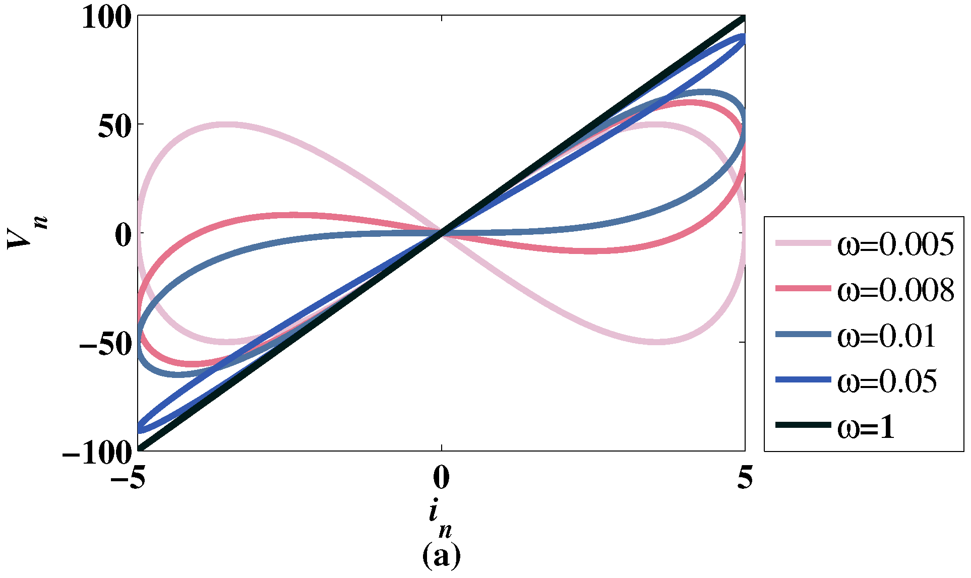
According to the experiment results of HP laboratory [17], set the current $i_n=Asin\left(\omega n\right)$ as the input, $A=5$, $q_0=0.1$, $k=1$. As $R_{off}\gg R_{on}$, the difference between $R_1$ and $R_2$ should be large. In this paper, $R_1=20$, $R_2=0.02$. Draw the curves of voltage changing with current as in Figure 1.

Different curves with different frequencies are shown in Figure 1. When the frequency increases gradually, the nonlinear relationship between current and voltage decreases. When $\omega =1$, the voltage increases linearly with the current. Figure 1 shows that model (7) conforms to the characteristics of the memristor under the above parameter values.

3. The Discrete Hyperchaotic Model with Variable Dimensions

3.1. Chaotic Model Construction Method

3.1.1. Cascade Operation

A cascade operation refers to connecting multiple associated objects. In computer applications, it can realize synchronous operation on multiple associated objects and improve efficiency. The cascade operation also has many applications in the construction of chaotic systems, and it has been proved to improve the complexity of chaos [33]. The basic form of cascade operation is

$$x_{n+1}=F\circ G\left(x_n\right)=F\left(G\left(x_n\right)\right),$$

(8)

where $F(·)$, $G(·)$ are two chaotic maps, ∘ denotes the cascade operation.

3.1.2. Coupling

In the design of circuits, if the current or voltage in one circuit changes, it can affect similar changes in other circuits. This network is called the coupling circuit. A similar operation can be used in the design of a chaotic system to realize combining several one-dimensional chaotic maps to a multi-dimensional chaotic system. The form of closed-loop coupling can be described as [34]

$$\left\{\begin{array}{c}{x}_1(t+1)=f_1(x_1\left(t\right),x_m\left(t\right))\hfill \\ x_2(t+1)=f_2(x_2\left(t\right),x_1(t+1))\hfill \\ ⋮\hfill \\ x_m(t+1)=f_m(x_m\left(t\right),x_{m-1}(t+1))\hfill \end{array}\right.$$

(9)

Based on this closed-loop coupling modulation, a novel coupling model with more related variables is designed as

$$\left\{\begin{array}{c}{x}_1(t+1)=f_1(x_1\left(t\right),x_m\left(t\right))\hfill \\ x_2(t+1)=f_2(x_2\left(t\right),x_1\left(t\right),x_1(t+1))\hfill \\ ⋮\hfill \\ x_m(t+1)=f_m(x_m\left(t\right),x_{m-1}\left(t\right),x_{m-1}(t+1))\hfill \end{array}\right.$$

(10)

Different from the coupling mode in (8), when calculating the value of the current time of a dimension, in addition to considering the influence of the value of the previous dimension at the current time, the influence of the previous dimension on the previous iteration result is also added. By adding the time-delayed variables, the coupling degree is increased, and the complexity of the system is improved.

3.2. The Coupling Model Based on Logistic Map and Sine Map (CLS)

An m-dimensional discrete hyperchaotic model combining cascade and time-dependent closed-loop coupling can be described as

$$\left\{\begin{array}{c}{x}_1(t+1)=f\circ g_1(x_1\left(t\right),x_m\left(t\right))\hfill \\ x_2(t+1)=f\circ g_2(x_2\left(t\right),x_1\left(t\right),x_1(t+1))\hfill \\ ⋮\hfill \\ x_m(t+1)=f\circ g_m(x_m\left(t\right),x_{m-1}\left(t\right),x_{m-1}(t+1))\hfill \end{array}\right.$$

(11)

Let $g_i(·)(i=1,2,\cdots ,m)$ be the Logistic map, and $f(·)$ be the Sine map. To increase the complexity of the Sine map, an exponential map is added to the Sine map as the frequency of the Sine map. The chaotic model can be constructed as

$$\left\{\begin{array}{c}{x}_1(t+1)=sin\left(b\frac{\mu x_1\left(t\right)(1-x_m\left(t\right))}{\epsilon e^{a{x}_m^2\left(t\right)}}\right)\hfill \\ x_2(t+1)=sin\left(b\frac{\mu x_2\left(t\right)(1-x_1\left(t\right))}{\epsilon e^{a{x}_1^2(t+1)}}\right)\hfill \\ ⋮\hfill \\ x_m(t+1)=sin\left(b\frac{\mu x_m\left(t\right)(1-x_{m-1}\left(t\right))}{\epsilon e^{a{x}_{m-1}^2(t+1)}}\right)\hfill \end{array}\right.,$$

(12)

where a, b, $\mu$, and $ϵ$ are parameters of system (11), and m is the dimension of the system.

The discrete memristor-based coupling model with a Logistic map and Sine map (MCLS) is

$$\left\{\begin{array}{c}{x}_1(t+1)=sin\left[b\frac{\mu (R_1-R_2(q_0+k\sum _{j=1}^t{x}_j))x_1\left(t\right)(1-x_m\left(t\right))}{\epsilon e^{a{x}_m^2\left(t\right)}}\right]\hfill \\ x_2(t+1)=sin\left[b\frac{\mu x_2\left(t\right)(1-x_1\left(t\right))}{\epsilon e^{a{x}_1^2(t+1)}}\right]\hfill \\ ⋮\hfill \\ x_m(t+1)=sin\left[b\frac{\mu x_m\left(t\right)(1-x_{m-1}\left(t\right))}{\epsilon e^{a{x}_{m-1}^2(t+1)}}\right]\hfill \end{array}\right.$$

(13)

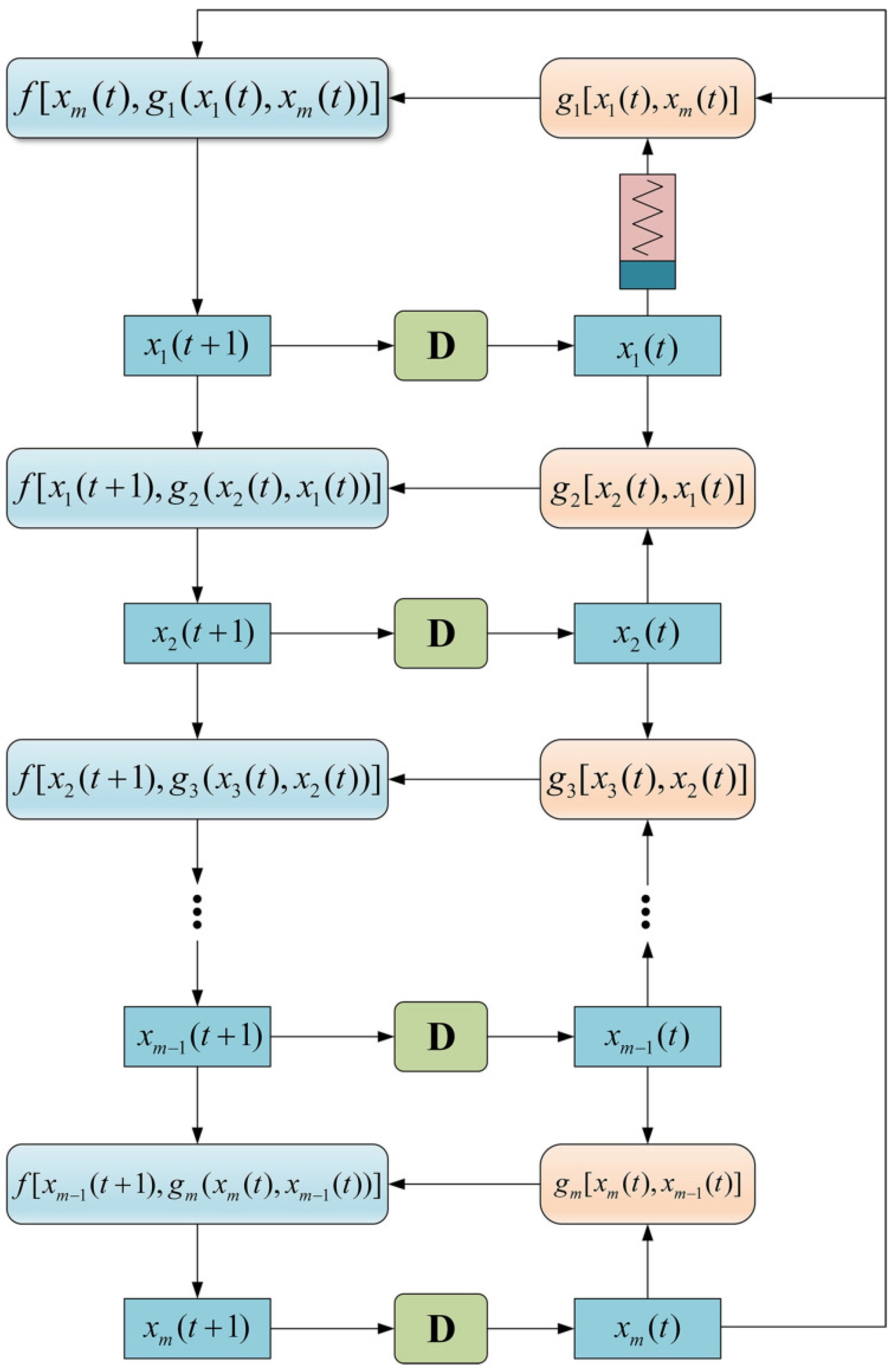
The structure of MCLS is shown in Figure 2.

4. Performances Analysis of CLS and MCLS

In the simulation experiments, to simplify the calculation, two-dimensional CLS and MCLS are taken as an example. All the analyses are based on the 2D-CLS and 2D-MCLS. Set $a=0.5$, $b=\pi$, $\mu =3$, $\epsilon =0.03$, $R_1=20$, $R_2=0.02$, $q_0=0.1$, $k=1$, and the initial values are $x_1\left(0\right)=0.3$, $x_2\left(0\right)=0.4$. Additionally, the simulation experiments are all conducted in MATLAB. The result of simulation experiments are shown in the following subsections.

4.1. Dynamic Performance in the Phase Space

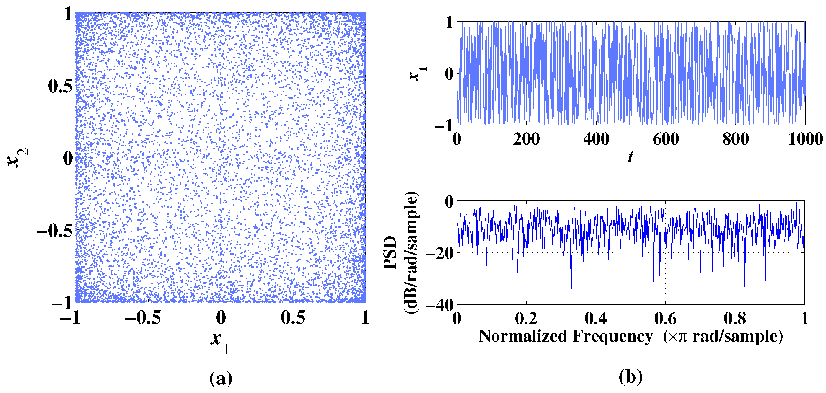
When taking different parameters, 2D-CLS and 2D-MCLS can produce different forms of sequence point distribution in phase space [35]. Set the parameters of CLS as $(\mu ,a,b,ϵ)=(3,0.5,\pi ,1.85)$, $(\mu ,a,b,ϵ)=(3,0.3,\pi ,1.85)$, $(\mu ,a,b,ϵ)=(3,0.5,\pi ,0.03)$, respectively. The initial value $(0.3,0.4)$ is substituted into 2D-CLS. Additionally, the computing time is set to $t=2100$ (in the experiment of the paper assumed to be in second). Remove the first 2000 iterations to obtain the distribution of the sequence in the phase space with the condition of three different parameter values set above. The corresponding time series and frequency spectrum in the time range of $[0,1000]$ is also calculated to observe the dynamic performance. The three types of dynamic behaviors of 2D-CLS are shown in Figure 3, Figure 4 and Figure 5.

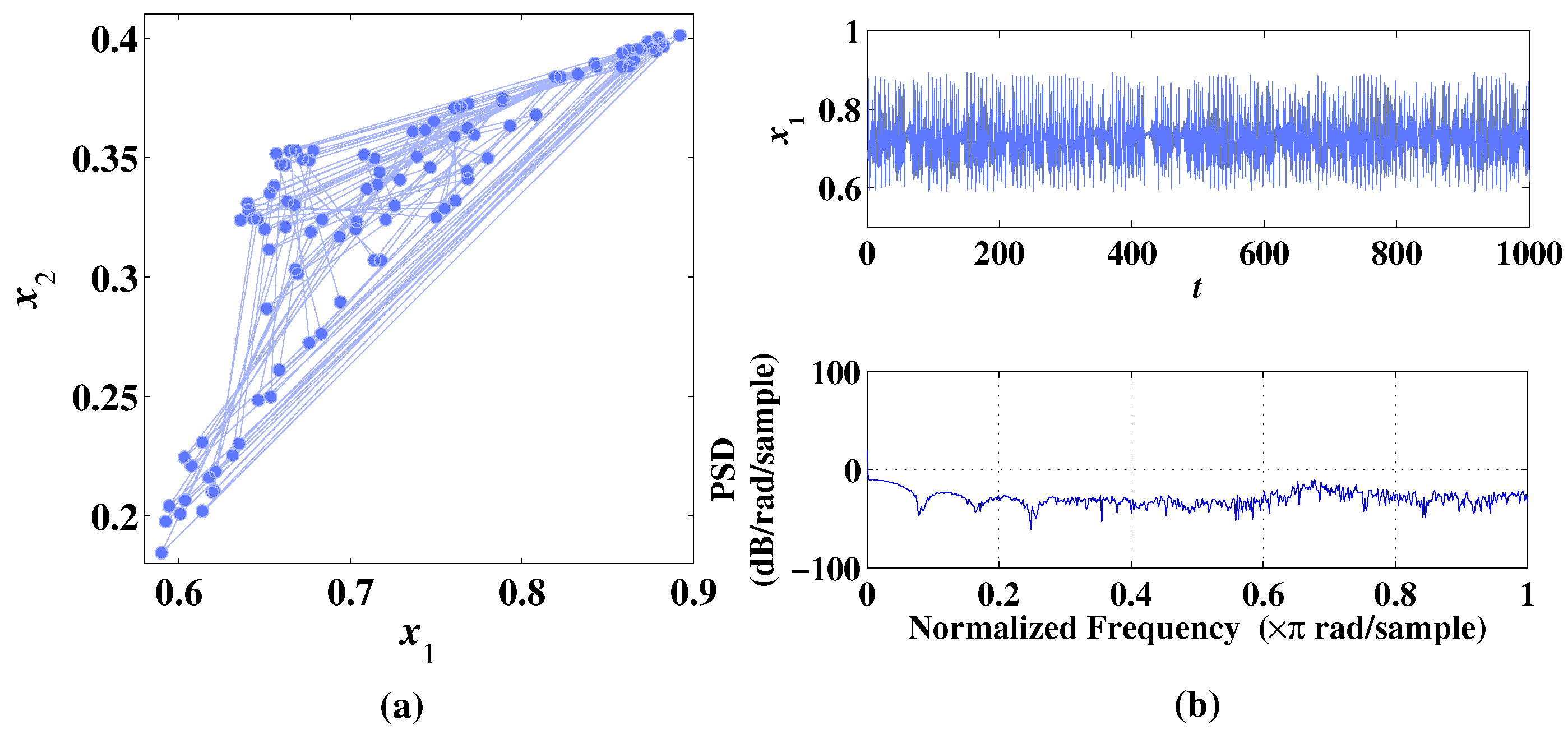
As shown in Figure 3a, the 2D-CLS can generate a chaotic attractor in a small range of $\left\{(x_1,x_2)\left|x_1\in (0.5,1),x_2\in (0.1,0.4)\right.\right\}$. In Figure 3b, the randomness of the sequence is reflected by the temporal diagram and frequency spectrum. The Lyapunov exponents at the chaotic state are $L{E}_1=0.5995$, and $L{E}_2=-0.0126$, which proves that the 2D-CLS can generate a chaotic attractor under the condition of $(\mu ,a,b,ϵ)=(3,0.5,\pi ,1.85)$.

As shown in Figure 4a, when $\mu =3,a=0.3,b=\pi ,ϵ=1.85$, two circular curves can be obtained by the 2D-CLS. As shown in Figure 4b, through the temporal diagram and frequency spectrum, it is concluded that the 2D-CLS system is in a periodic state. Calculate the Lyapunov exponents of 2D-CLS in this state as $L{E}_1=-0.0089,L{E}_2=-0.1742$, which shows that 2D-CLS is non-chaotic under the condition of $(\mu ,a,b,ϵ)=(3,0.3,\pi ,1.85)$.

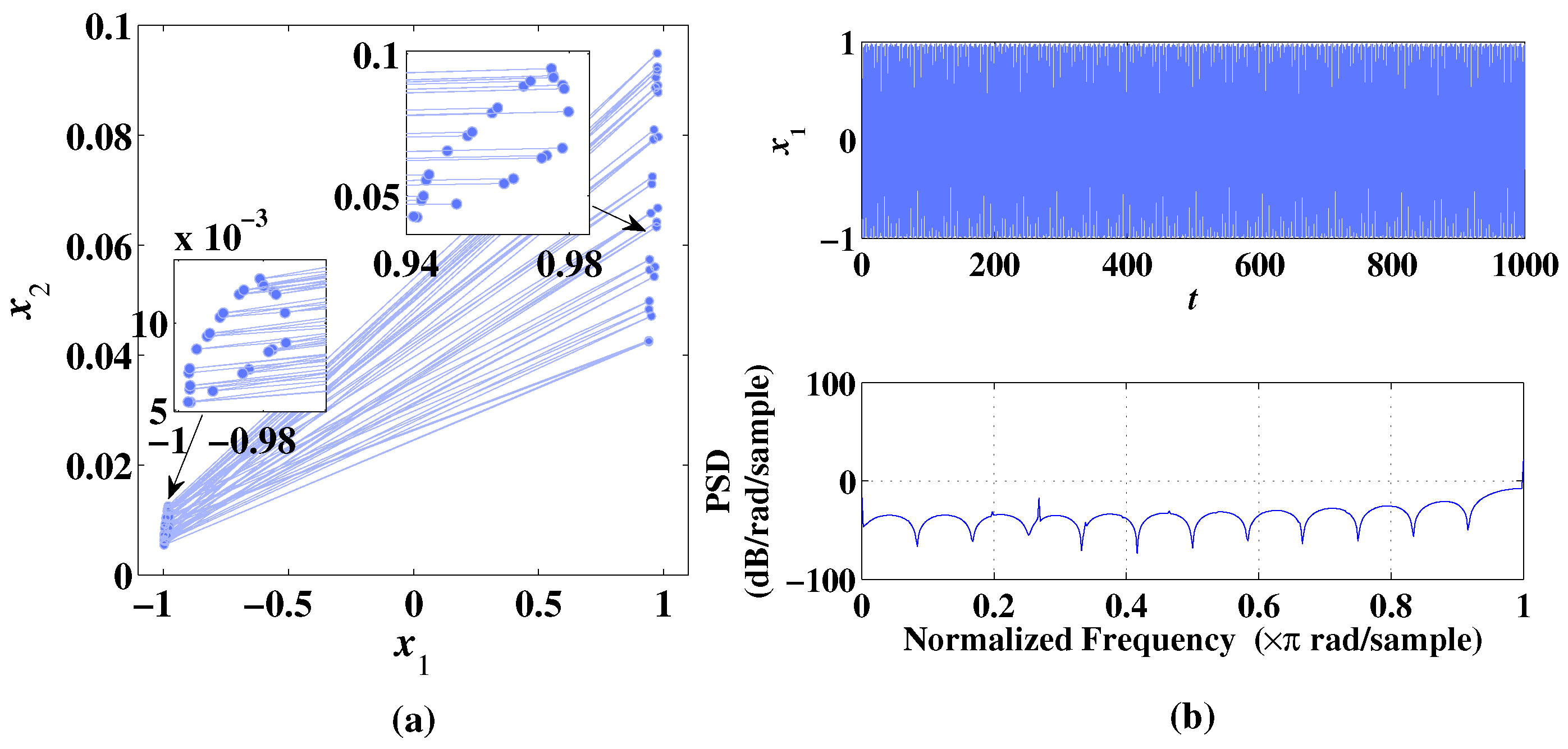
When $\mu =3,a=0.5,b=\pi ,ϵ=0.03$, the sequences of 2D-CLS can be evenly and irregularly distributed in the phase space with no obvious trajectory as shown in Figure 5a. It is shown that the system does not produce an attractor at this parameter value. In Figure 5b, the sequence can be distributed irregularly with the change in time and frequency. The Lyapunov exponents are calculated as $L{E}_1=5.0943,L{E}_2=4.2186$, showing that the 2D-CLS is hyperchaotic. This type of state is common in 2D-CLS with the change of parameters, which will be shown in the Lyapunov exponents and bifurcation diagram analysis in the following section.

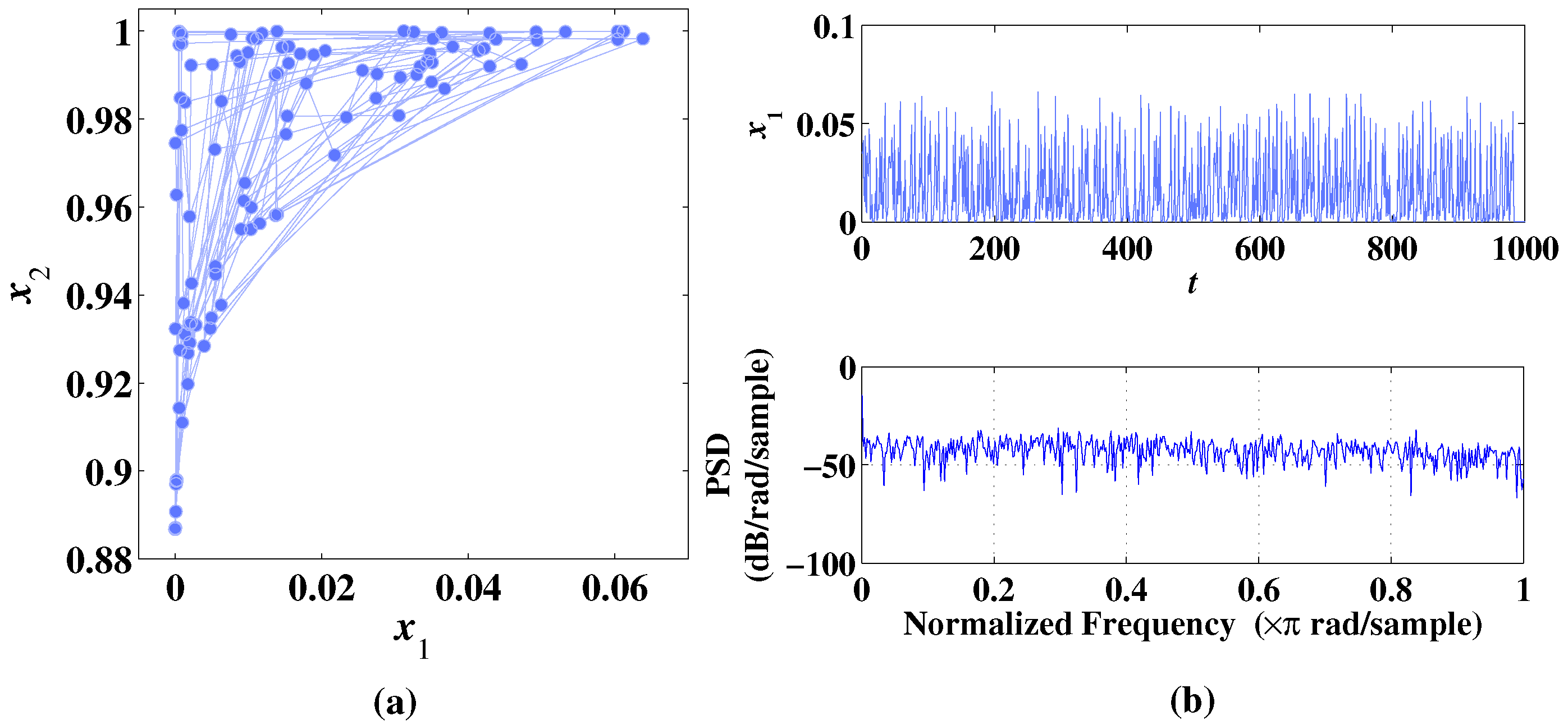
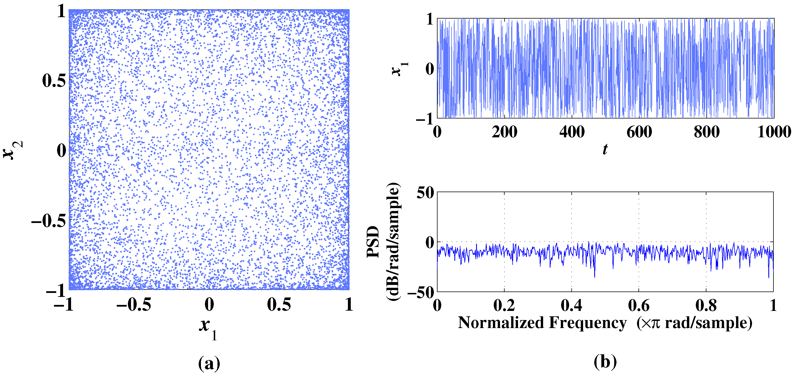
Correspondingly, the dynamic behaviors of 2D-MCLS under the condition of $(\mu ,a,b,ϵ)=(3,0.5,\pi ,1.13)$, $(\mu ,a,b,ϵ)=(0.02,0.3,\pi ,0.03)$, and $(\mu ,a,b,ϵ)=(3,0.5,\pi ,0.03)$ are shown in Figure 6, Figure 7 and Figure 8.

When the discrete memristor is added to the 2D-CLS system, the dynamic characteristics are changed. When $(\mu ,a,b,ϵ)=(3,0.5,\pi ,1.13)$, the 2D-MCLS does not present the chaotic attractor shown in Figure 3a. However, another form of an attractor is generated as in Figure 6a with the parameter changing to 1.13. As shown in Figure 6b, the temporal diagram and frequency spectrum present certain randomness in the sequence. The corresponding Lyapunov exponents are $L{E}_1=0.7846,L{E}_2=0.5003$.

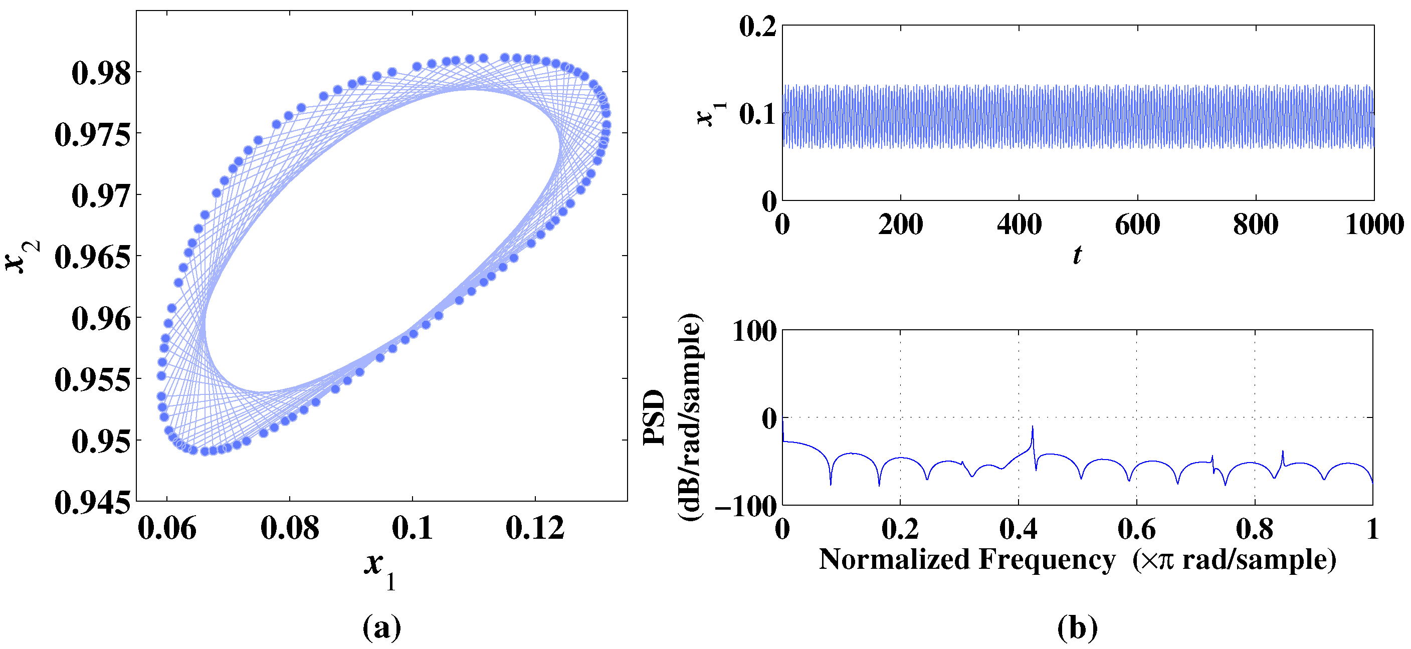
As shown in Figure 7a, when $(\mu ,a,b,ϵ)=(0.02,0.3,\pi ,0.03)$, the sequences generated by 2D-MCLS form a circular curve in the ranges of $x_1\in (0.05,0.15),x_2\in (0.94,0.99)$. As shown in Figure 7b, the temporal diagram and frequency spectrum show obvious periodicity. Additionally, the Lyapunov exponents are computed as $L{E}_1=-0.0092,L{E}_2=-0.0851$, which proves that the 2D-MCLS is non-chaotic at this condition of parameters.

In Figure 8a, when $(\mu ,a,b,ϵ)=(3,0.5,\pi ,0.03)$, 2D-MCLS generates evenly distributed chaotic sequences without obvious trajectory. In Figure 8b, the sequence is irregular with the change in time and frequency. The Lyapunov exponents are calculated as $L{E}_1=7.3724,L{E}_2=4.9317$, showing that the 2D-MCLS system is hyperchaotic under this condition of parameters.

4.2. Evolution of the CLS and MCLS with the Variation of Parameters

The Lyapunov exponents (LEs) can judge whether the system is chaotic or not. A positive Lyapunov exponent represents expanding nature, and the system is chaotic [36]. If there are two or more positive Lyapunov exponents, the system is hyperchaotic [37]. By calculating LEs with varying parameters, the evolution of systems with the variation of parameters can be accurately described [38,39]. Correspondingly, the bifurcation diagram can show the distribution change of the chaotic sequence with the change of the parameters directly. The dynamic performances of CLS and MCLS with changing parameters are analyzed in the following sections.

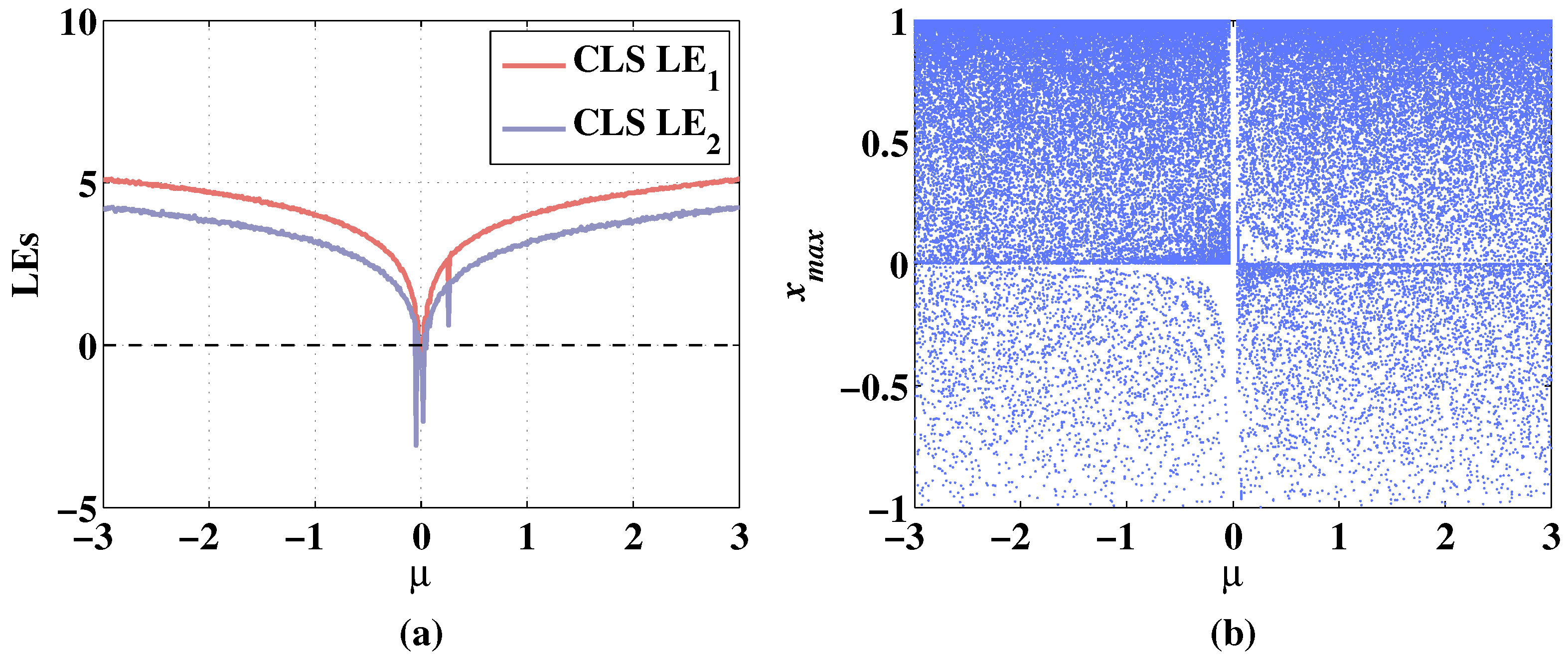
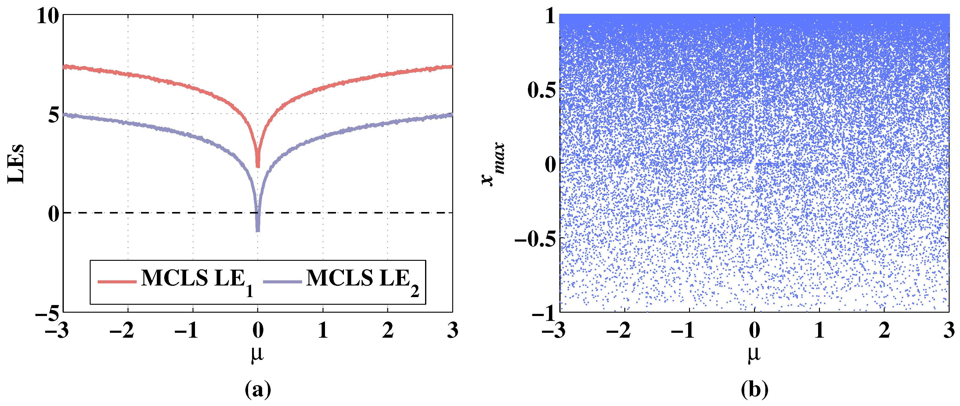
Set the parameters $(a,b,ϵ)=(0.5,\pi ,0.03)$ and input the initial values $x_1\left(0\right)=0.3,$$x_2\left(0\right)=0.4$ to the 2D-CLS system and 2D-MCLS system, respectively. Iterate 2000 times to get the chaotic sequences, which are used to calculate the Lyapunov exponents and to depict the bifurcation diagram. The step of parameter variation is 0.01. By calculating the values of LEs, it can be found that when the value of $\mu$ is close to 0, the state of the system changes with the change of $\mu$. When the absolute value of $\mu$ increases, the systems remain hyperchaotic. To compare the state variations of 2D-CLS and 2D-MCLS, a range of $\mu$ with $(-3,3)$ is chosen. The LEs and bifurcation diagrams of 2D-CLS and 2D-MCLS changing with the parameter $\mu$ are compared in Figure 9 and Figure 10.

The Lyapunov exponents and bifurcation diagrams of the 2D-CLS and 2D-MCLS show a symmetrical increasing trend with the increase of the absolute value of $\mu$. In Figure 9a, when $\mu$ is taken between $[-0.05,0.02]$, the LEs of 2D-CLS are negative. The 2D-CLS system stays hyperchaotic when $\mu$ decreases from −0.05 to −3. The $L{E}_1$ increases to bigger than 0 when $\mu$ is greater than 0.02. The $L{E}_2$ increases to bigger than 0 when $\mu$ is greater than 0.04. In Figure 9b, it can be seen that the 2D-CLS system is in a periodic state when $\mu$ is taken between [−0.05,0.02]. In Figure 10a, with the addition of a discrete memristor, the whole level of LEs is improved. The $L{E}_1$ is positive in the range of $\mu$. The $L{E}_2$ is negative when $\mu$ is taken between $[-0.02,0.02]$ and it is bigger than 0 when the absolute value of $\mu$ is greater than 0.02. As shown in Figure 10b, the 2D-MCLS shows periodic states when $\mu$ is varying from −0.02 to 0.02 and it remains chaotic with the parameter $\mu$ changes in other ranges.

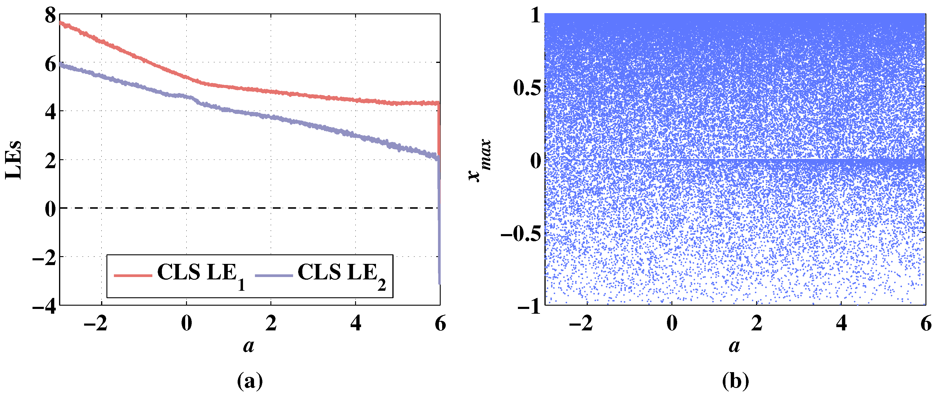
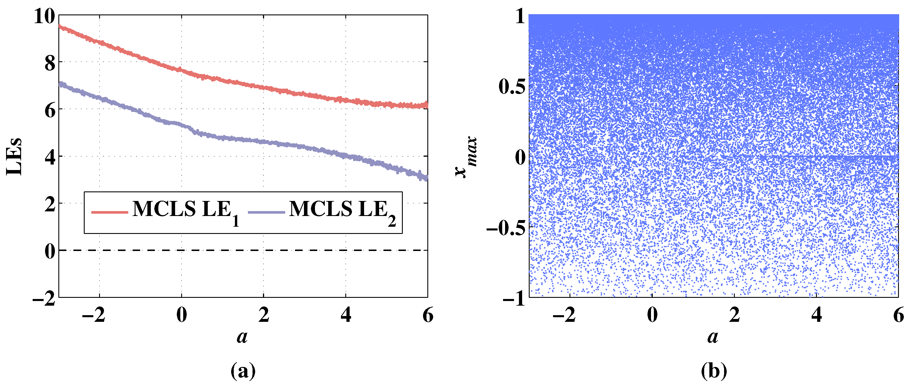
Set the parameters $(\mu ,b,ϵ)=(3,\pi ,0.03)$ and input the initial values $x_1\left(0\right)=0.3,x_2\left(0\right)=0.4$ to the 2D-CLS and 2D-MCLS, respectively. Iterate 2000 times to get the curves of LEs and bifurcation diagrams. The results are shown in Figure 11 and Figure 12.

In Figure 11a, the 2D-CLS remains hyperchaotic with the change of parameter a between $[-3,5.97]$, and the LEs decreases with the parameter a increasing. The LEs are negative when the parameter a increases from 5.98 to 6. In Figure 11b, the sequence is chaotic with the variation of a. As shown in Figure 12a, the LEs are also increasing with the parameter a decreasing. Additionally, the LEs are higher than the 2D-CLS. There are no negative points of LEs with the variation of a. In Figure 12b, the sequence of 2D-MCLS is hyperchaotic with the change of parameter a.

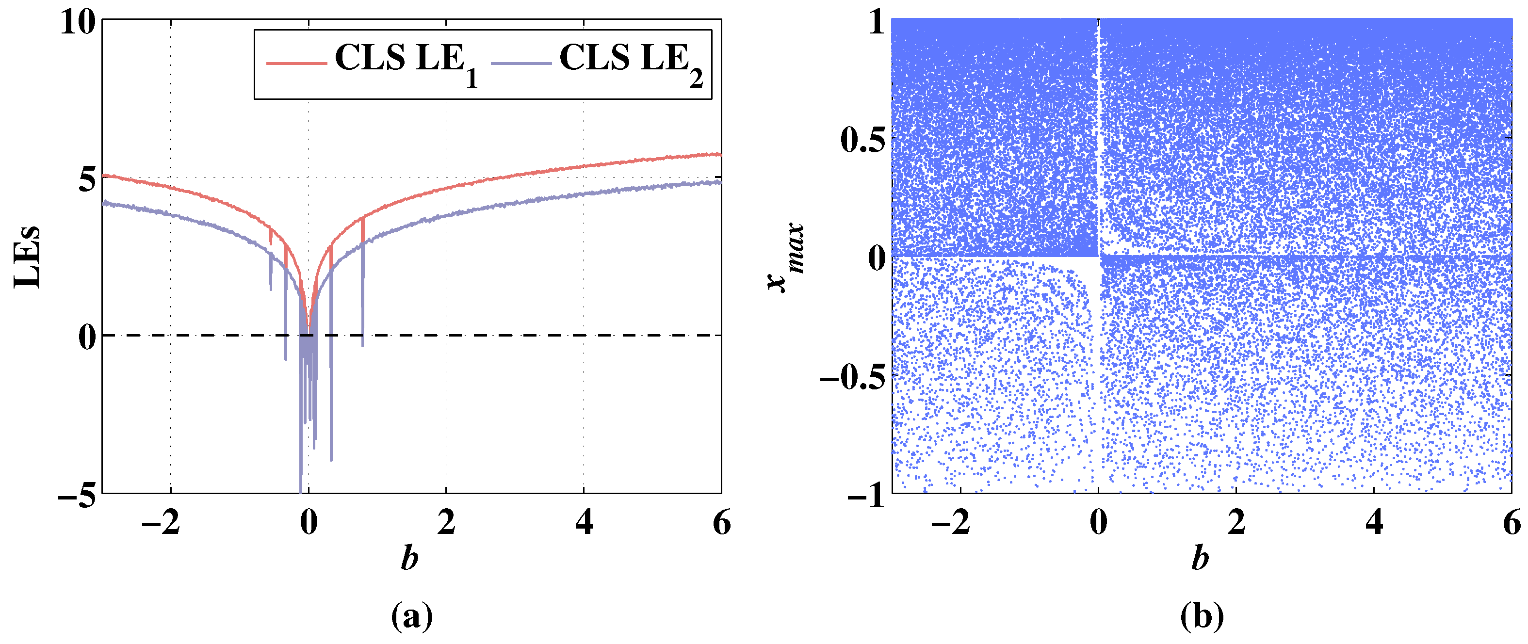
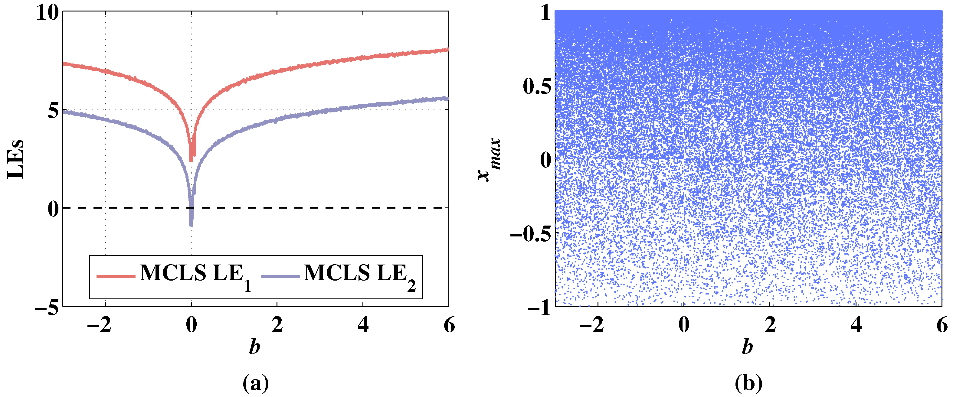
Set the parameters $(\mu ,a,ϵ)=(3,0.5,0.03)$ and calculate the sequences of CLS system and MCLS system with the initial value $x_1\left(0\right)=0.3,x_2\left(0\right)=0.4$. The length of each sequence is 2000. The step of parameter variation is 0.01. Then the LEs and the bifurcation diagrams changing with parameter b are shown in Figure 13 and Figure 14.

As shown in Figure 13a, the system state shows symmetry with the change of parameter b. In the range of $[-0.33,0.33]$, the LEs corresponding to several parameter value points are negative. It shows a stable hyperchaotic state when parameter b is less than −0.33 or greater than 0.79. As shown in Figure 13b, there is a periodic window in the range of $(-0.03,0.03)$, and the sequence of 2D-CLS remains chaotic when the parameter b increases from 0.03 or decreases from −0.03. As the discrete memristor is added to the system, the level of LEs is improved in the range of $[-3,6]$ as shown in Figure 14a. The $L{E}_1$ stays positive with the variation of parameter b. Additionally, the $L{E}_2$ begins to be bigger than 0 when the parameter b is greater than 0.05. As shown in Figure 14b, the sequence of 2D-MCLS is chaotic with the change of parameter b. As shown in Figure 13 and Figure 14, the Lyapunov exponents and bifurcation diagrams of the 2D-CLS and 2D-MCLS show a symmetrical increasing trend with the increase of the absolute value of b.

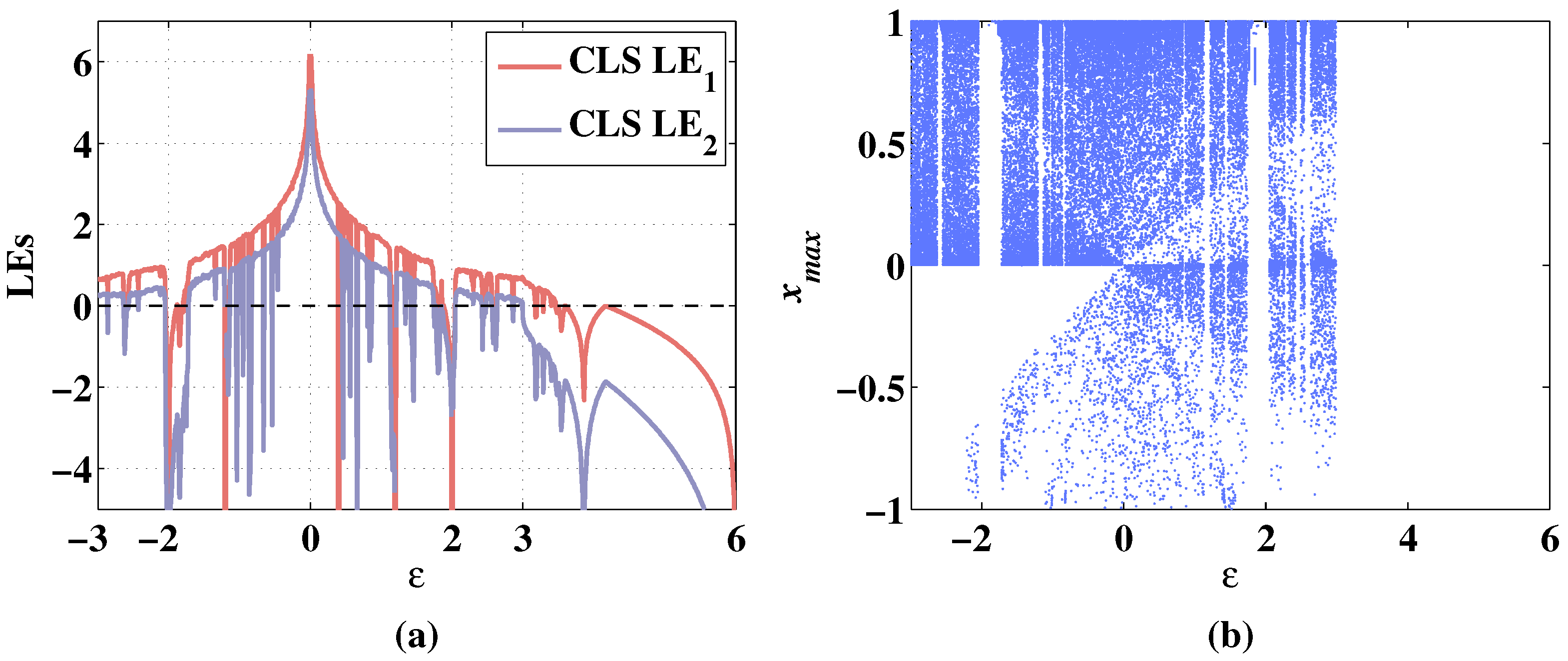
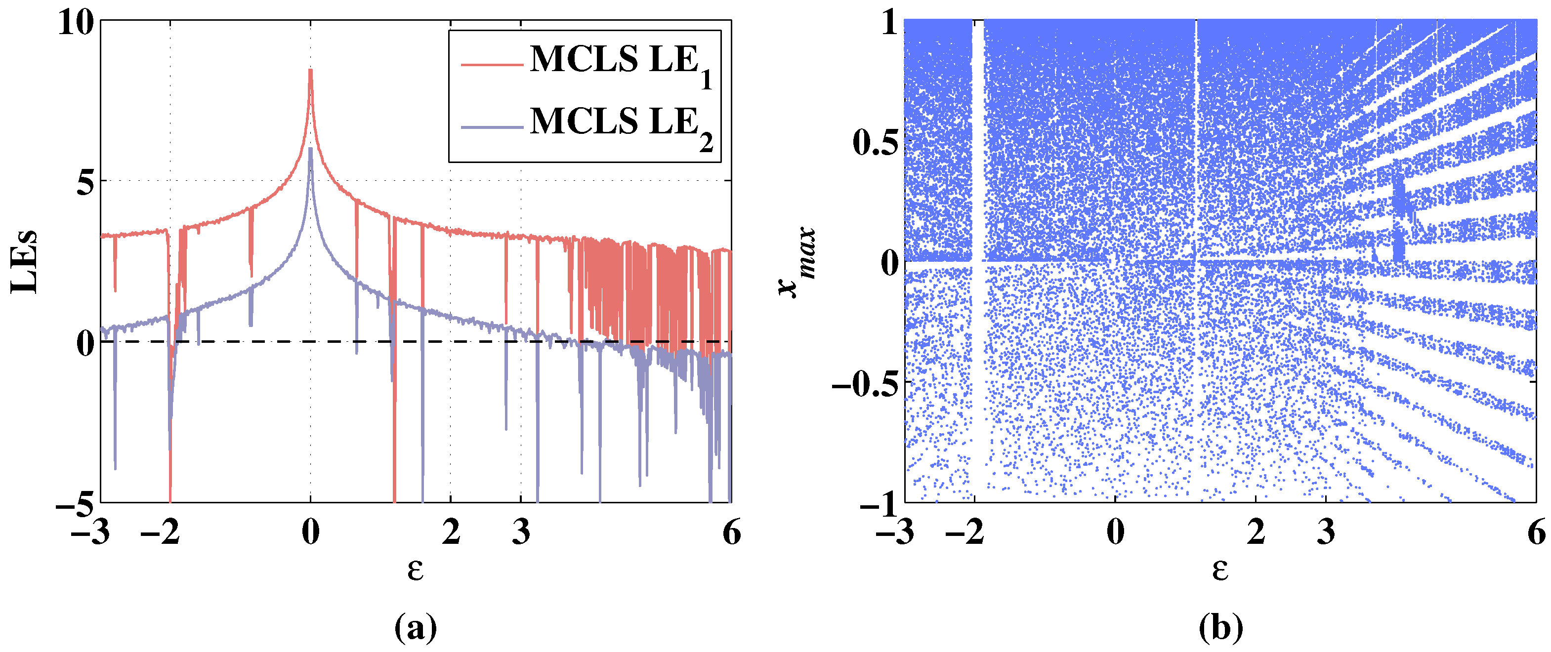
Set the parameters $(\mu ,a,b)=(3,0.5,\pi )$ and input the initial values $x_1\left(0\right)=0.3,x_2\left(0\right)=0.4$ to the 2D-CLS system and 2D-MCLS system, respectively. Iterate 2000 times to calculate sequences to get the curves of LEs and the bifurcation diagrams. The results are shown in Figure 15 and Figure 16.

As shown in Figure 15a, the change of the system state with the variation of $ϵ$ is also symmetrical. In the range where $ϵ$ is greater than 0, the $L{E}_1$ becomes negative when $ϵ$ increases to 0.4. In the range where $ϵ$ is smaller than 0, the $L{E}_1$ becomes negative when $ϵ$ decreases to −0.66. Additionally, the $L{E}_2$ remains negative when $ϵ$ is taken from the range of $[3,6]$. As shown in Figure 15b, the sequence of 2D-CLS is chaotic while parameter $ϵ$ changes from −0.66 to 0.4. There are several periodic windows when the parameter $ϵ$ is greater than 0.56 or smaller than −0.66. Additionally, the value of the sequence remains 0 when $ϵ$ increases from 3 to 6 although the $L{E}_1$ is positive, which shows that the 2D-CLS fails to expand the dimension with chaotic states with parameter $ϵ$ taken from $[3,6]$. As shown in Figure 16a, 2D-MCLS remains hyperchaotic when $ϵ$ changes in the range of $(-1.6,0.66)$. Additionally, in Figure 16b, there are only two periodic windows in the range of $[-2.02,-1.92]$ and $[1.16,1.2]$, respectively. Additionally, in the range of $[3,6]$, the sequence of 2D-MCLS is generally chaotic. The Lyapunov exponents and bifurcation diagrams of the 2D-CLS and 2D-MCLS show a symmetrical decreasing trend with the increase of the absolute value of $ϵ$.

4.3. Global Dynamics Analysis Based on Lyapunov Exponents

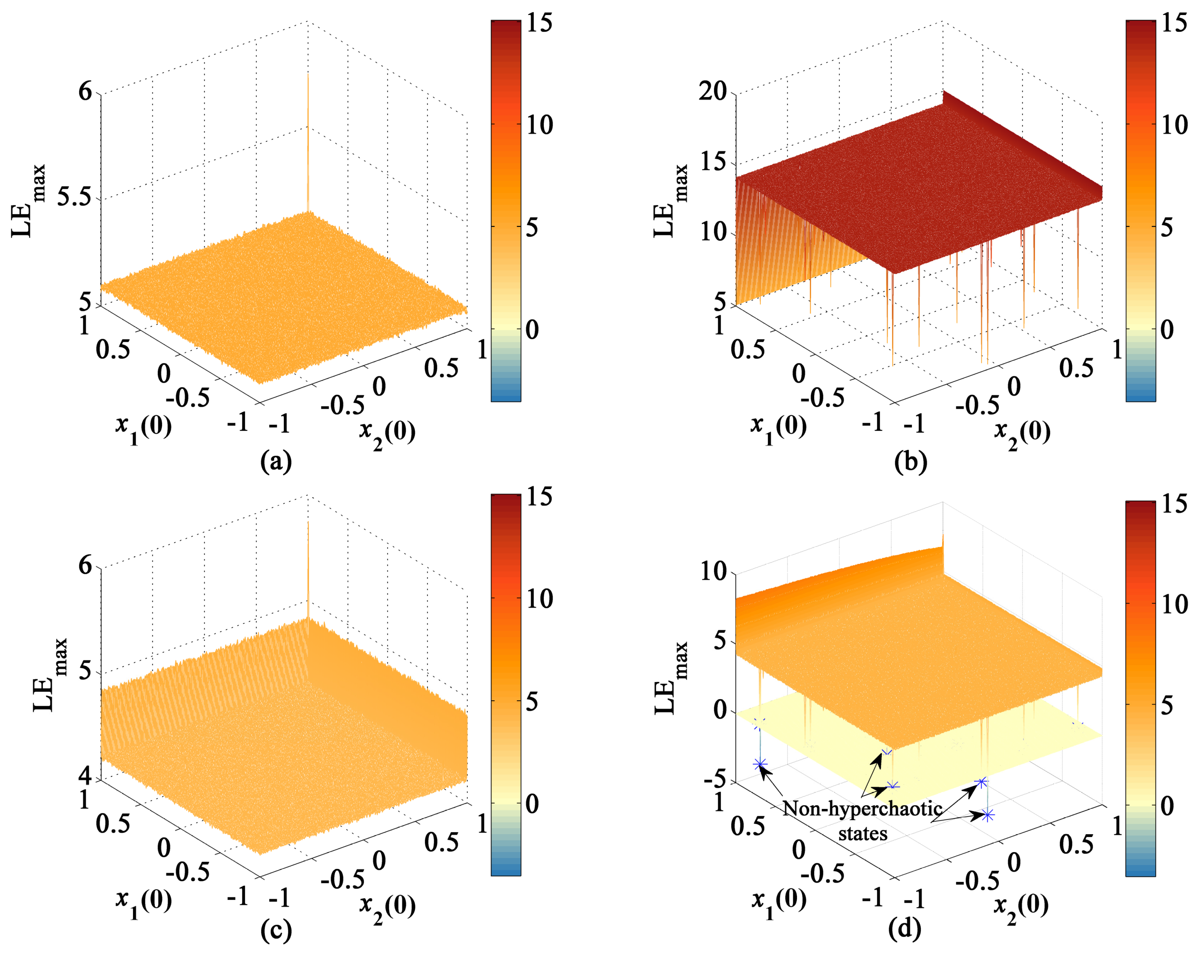
By calculating LEs for the values within the whole initial value range, the influence of the initial value change on the dynamics performance of the system can be comprehensively investigated. By comparing the global dynamic characteristics of CLS and MCLs based on initial values, it can explore the influence of discrete memristor on the CLS model.

The range of initial values of the CLS and MCLS is $x_1\left(0\right),x_2\left(0\right)\in [-1,1]$. Take 300 points from the ranges and calculate the LEs as shown in Figure 17. According to Figure 17a,b, the values of the first LE are positive in the whole range. Additionally, the first LE of MCLS higher than the CLS’s except that LE of some initial value points is relatively low. Similarly, in Figure 17c,d, the second LE of MCLS is higher than that of CLS. However, in Figure 17d, the diagram of the second LE of MCLS displays some points that are under the zero plane and show negative values of the second LE, which explain that the MCLS is non-hyperchaotic.

4.4. The Complexity Analysis

4.4.1. The Permutation Entropy

The permutation entropy (PE) [40] can measure the complexity of a sequence. For a one-dimensional sequence x with length N, reconstruct the sequence into a new sequence with n-dimensional and lag time of $\tau$

$$X\left(t\right)={[x\left(t\right),x(t+\tau ),\cdots ,x(t+(n-1)\tau )]}^T.$$

(14)

Then PE is defined as

$$H\left(n\right)=-\sum _{i=1}^{n!}P\left({\pi }_i\right)logP\left({\pi }_i\right).$$

(15)

where $P\left({\pi }_i\right)$ is the occurrence probability of the ith type of permutation of n different number. For a random sequence, the probability of all possible permutations of the numbers in the sequence is equal, and the value of PE should be 1. If the PE of the sequence is close to 1, it means that the sequence is highly random.

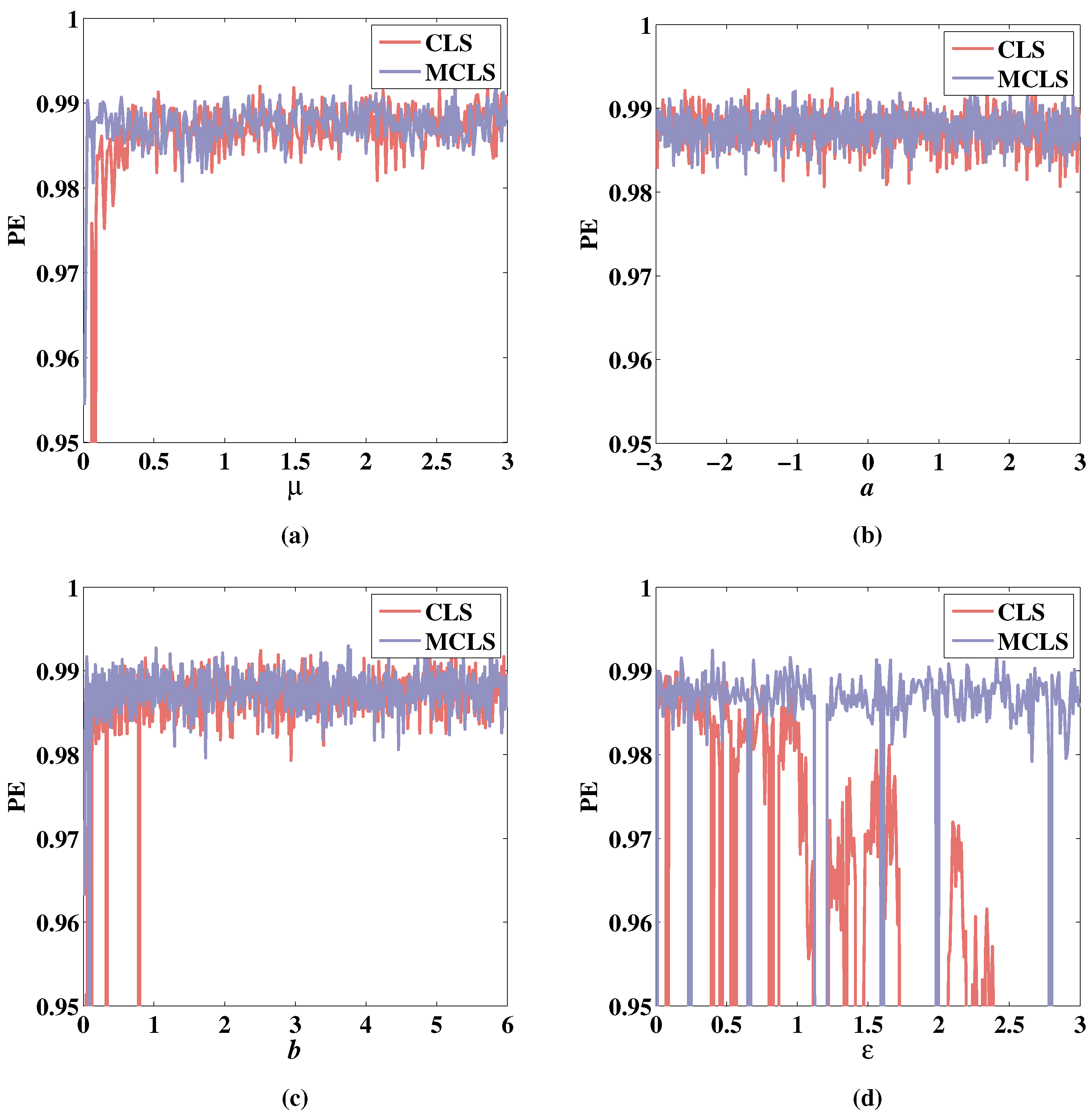
Choose the $x_1$ sequence to calculate the PE value varying with the four parameters, respectively. The results are shown in Figure 18.

As shown in Figure 18a–c, the PE increases while $\mu$ and b increase, and the PE of MCLS increases more rapidly. Additionally, Figure 18d shows that the PE of CLS decreases when parameter $ϵ$ increases but the PE of MCLS is relatively maintained close to 1 except for a few dropping points. It can be seen from the analysis above that the changes in the Lyapunov exponent, bifurcation diagram, and PE diagram are corresponding.

4.4.2. The Spectral Entropy Complexity

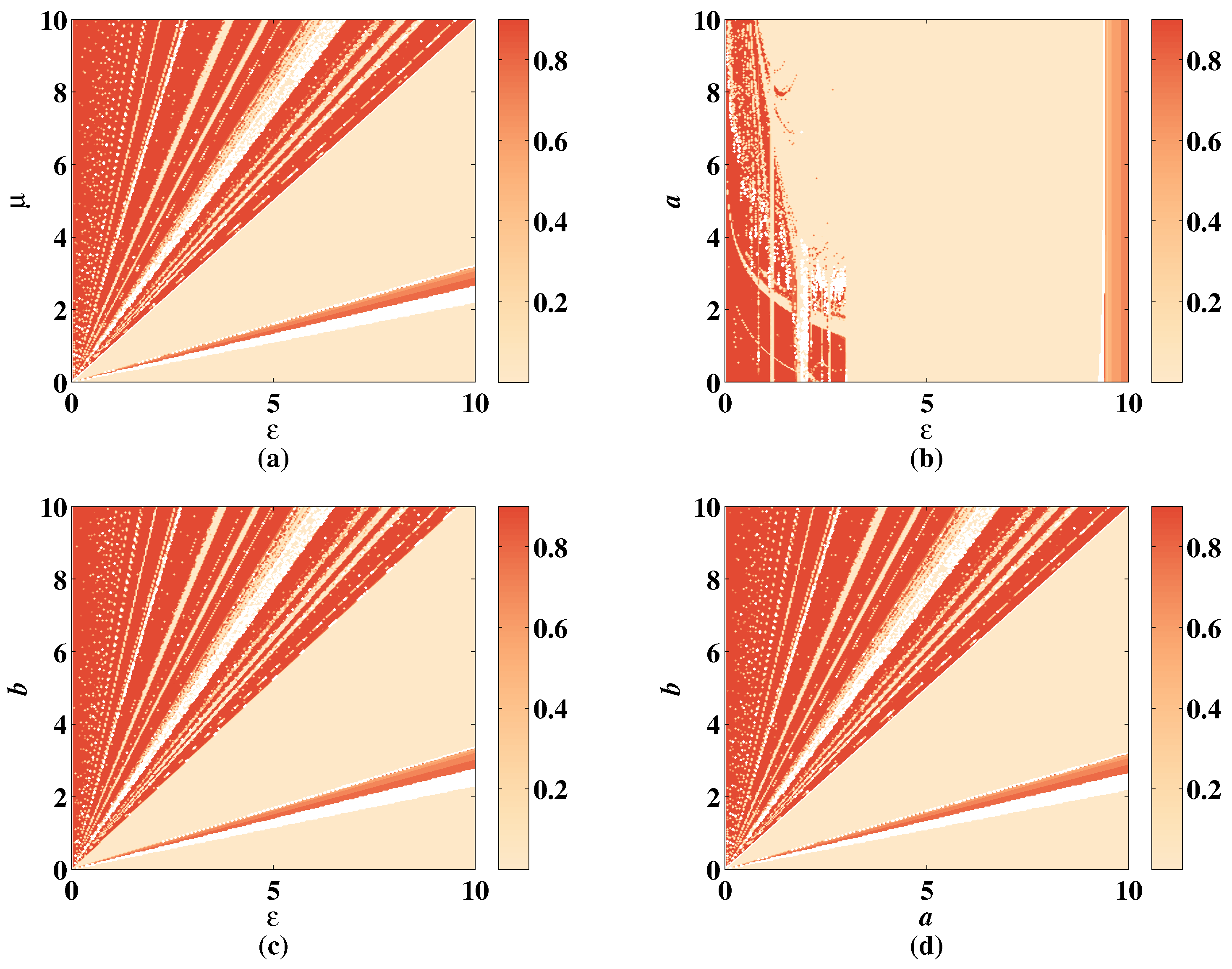
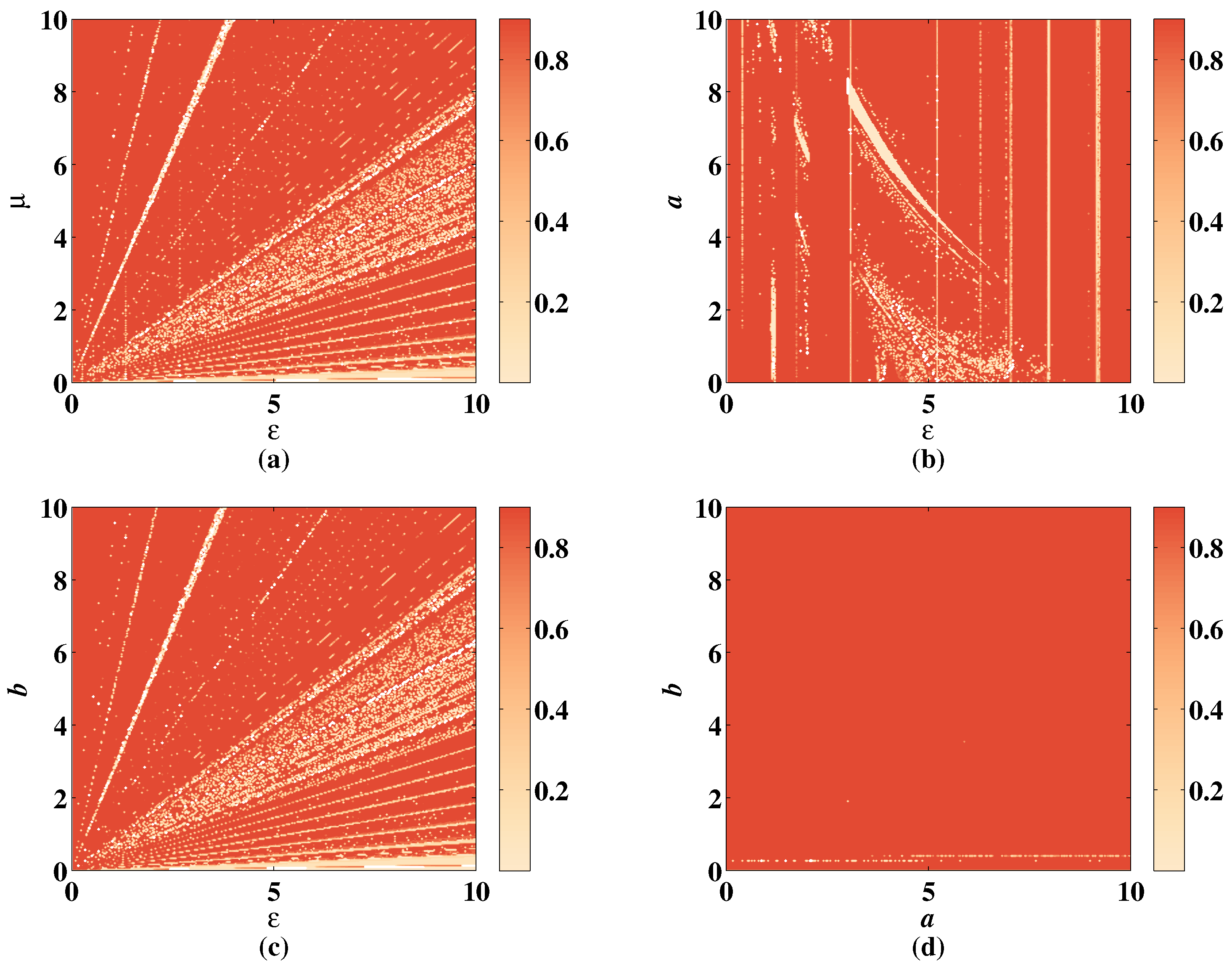
Spectral entropy is another method to measure the complexity of sequences, which reflects the randomness of the sequence from the perspective of the energy spectrum. The value range of spectral entropy is between $[0,1]$. The closer the value is to 1, the more stable the energy spectrum is and the better the randomness of the sequence is. Take 300 values for each parameter, and calculate the spectral entropy for CLS and MCLS, respectively, as shown in Figure 19 and Figure 20.

As shown in Figure 19a–c, the color distribution is relatively even, changing with parameters $\mu$, a, and b, but the color is shallow in the right part of the figures due to the unstable parameter $ϵ$. The SE stays value when increasing the value of $ϵ$. In Figure 19b, when $ϵ$ is set in the range $[3,10]$, the SE value is low whatever a changes. In Figure 19d, the lower right corner shows the low complexity of CLS. These shallow regions are filled with deep color when adding the discrete memristor shown in Figure 20. The simulation result shows that under the influence of discrete memristor, the complexity of hyperchaotic sequence is improved, and the range of hyperchaotic system parameters is larger.

4.5. The 0–1 Test

The 0–1 test was proposed by Gottwald and Melbourne to analyze the randomness of time series [41]. The calculation of 0–1 test does not need phase space reconstruction, which reduces the calculation time. Through the 0–1 test, the states of CLS and MCLS can be quickly judged. Two functions are defined as

$$\begin{array}{c}p\left(t\right)=\sum _{j=1}^t\varphi \left(j\right)cos\left(\theta \right(j\left)\right),t=1,2,\cdots ;\hfill \\ s\left(t\right)=\sum _{j=1}^t\varphi \left(j\right)sin\left(\theta \right(j\left)\right),t=1,2,\cdots ;\hfill \\ \theta \left(j\right)=jc+\sum _{i=1}^j\varphi \left(i\right),j=1,2,\cdots ,t.\hfill \end{array}$$

(16)

where $\varphi \left(i\right)$ is the ith value of the observed sequence, and c is a positive constant. In the paper, c is set to be 2. $p\left(t\right)$ and $s\left(t\right)$ are bounded if the sequence is non-chaotic. If $p\left(t\right)$ and $s\left(t\right)$ behave as Brownian motion, the sequence is chaotic. An index to distinguish the chaotic states is defined as

$$\begin{array}{c}K=\underset{t\to \infty }{lim}\frac{logM\left(t\right)}{logt};\hfill \\ M\left(t\right)=\frac{1}{T-t}\sum _{j=1}^{T-t}{\left[p\right(j+t)-p(j\left)\right]}^2.\hfill \end{array}$$

(17)

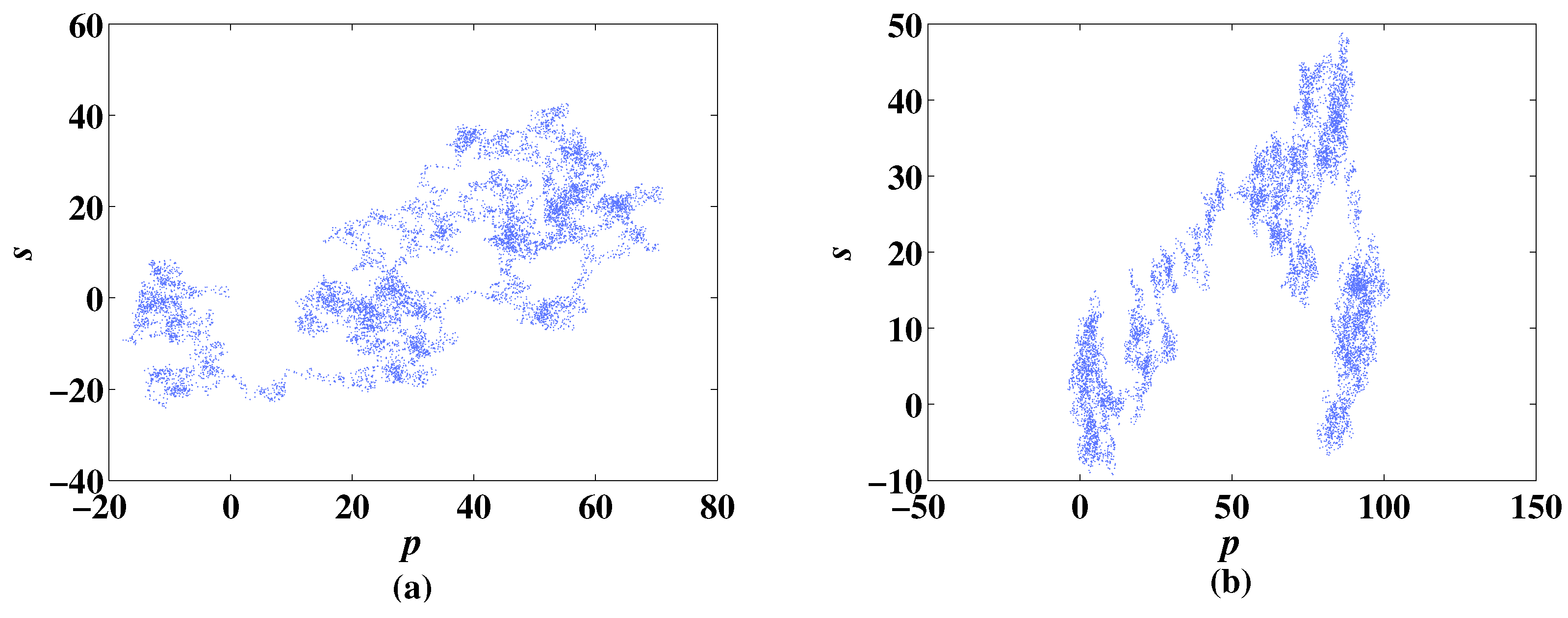
It can distinguish chaotic and non-chaotic states of sequences in binary form, in which $K=1$ denotes a chaotic state and $K=0$ denotes a non-chaotic state. Two variables $p\left(t\right)$ and $s\left(t\right)$ are calculated in the process of the 0–1 test to describe the motion track of the sequence. The track of the CLS system and the MCLS system with particulate parameter values are depicted in Figure 21a,b, respectively. The figures show that the $p-s$ track of the CLS and the MCLS system are both irregular, which reflects that the two systems are chaotic.

5. Discussion

In the above work, the proposed CLS model can effectively improve the complexity of the simple chaotic maps by constructing a new closed-loop coupling modulation. The added discrete memristor can further optimize the performance of discrete chaotic maps. These characteristics are of great value in the application of pseudo-random generator designs for information encryptions which needs larger keyspace and more random sequences. From the performance analysis of CLS, it can be concluded that the proposed closed-loop coupling modulation is effective. Based on this result, it is worth further exploration of the influence of time step variation on the chaotic system. The common shape without an attractor generated by the CLS and MCLS shows no obvious trajectory, but it is still bound in a certain range. This characteristic meets the need for encryption designs. The discrete form means that it is easy to realize hardware implementation as it does not need to solve differential equations. Further work is to conduct the hardware implementation to analyze the feasibility of this type of model.

6. Conclusions

In this paper, an improved time-dependent closed-loop coupling is proposed to design a dimension-changeable hyperchaotic CLS system. The discrete memristor is applied to improve the complexity of CLS. The dynamics performance analysis shows that the proposed method to construct discrete high-dimensional chaotic systems can generate a symmetrical distribution of LEs and bifurcation diagrams with variations of parameters. The randomness is effectively improved by the CLS. Additionally, the discrete memristor has played a great role in maintaining the stability of chaotic states with the variation of parameters. The proposed model with a discrete memristor shows a high value of the application for information encryption. The work conducted above is of great interest for further research on closed-loop coupling and the application of discrete memristors. Additionally, the hardware implementation would be realized in future work.

References

- Dai, W.; Xu, X.; Song, X.; Li, G. Audio Encryption Algorithm Based on Chen Memristor Chaotic System. Symmetry 2021, 14, 17. [Google Scholar] [CrossRef]
- Song, X.; Xu, D.; Li, G.; Xu, W. Multi-Image Reorganization Encryption Based on S-L-F Cascade Chaos and Bit Scrambling. J. Web Eng. 2021, 20, 1115–1130. [Google Scholar] [CrossRef]
- Zhong, H.; Li, G. Multi-Image Encryption Algorithm Based on Wavelet Transform and 3D Shuffling Scrambling. Multimed. Tools Appl. 2022, 1–20. [Google Scholar] [CrossRef]
- Li, G.; Xu, X.; Zhong, H. A image encryption algorithm based on coexisting multi-attractors in a spherical chaotic system. Multimed. Tools Appl. 2022, 1–27. [Google Scholar] [CrossRef]
- Chen, G.; Ueta, T. Yet Another Chaotic Attractor. Int. J. Bifurc. Chaos 1999, 9, 1465–1466. [Google Scholar] [CrossRef]
- Phatak, S.C.; Rao, S.S. Logistic Map: A Possible Random-Number Generator. Phys. Rev. E 1995, 51, 3670–3678. [Google Scholar] [CrossRef] [Green Version]
- Zhang, Q.; Xiang, Y.; Fan, Z.; Bi, C. Study of Universal Constants of Bifurcation in a Chaotic Sine Map. In Proceedings of the 2013 Sixth International Symposium on Computational Intelligence and Design, ISCID 2013, Hangzhou, China, 28–29 October 2013; Volume 2, pp. 177–180. [Google Scholar]
- Alawida, M.; Samsudin, A.; Teh, J.S.; Alkhawaldeh, R.S. A New Hybrid Digital Chaotic System with Applications in Image Encryption. Signal Process. 2019, 160, 45–58. [Google Scholar] [CrossRef]
- Hua, Z.; Zhou, Y.; Huang, H. Cosine-Transform-Based Chaotic System for Image Encryption. Inf. Sci. 2019, 480, 403–419. [Google Scholar] [CrossRef]
- Khalil, N.; Sarhan, A.; Alshewimy, M.A.M. An Efficient Color/Grayscale Image Encryption Scheme Based on Hybrid Chaotic Maps. Opt. Laser Technol. 2021, 143, 107326. [Google Scholar] [CrossRef]
- Wu, C.; Sun, K.; Xiao, Y. A Hyperchaotic Map with Multi-Elliptic Cavities Based on Modulation and Coupling. Eur. Phys. J. Spec. Top. 2021, 230, 2011–2020. [Google Scholar] [CrossRef]
- Wu, Q. Cascade-Sine Chaotification Model for Producing Chaos. Nonlinear Dyn. 2021, 106, 2607–2620. [Google Scholar] [CrossRef]
- Zhao, Z.P.; Zhou, S.; Wang, X.Y. A New Chaotic Signal Based on Deep Learning and Its Application in Image Encryption. Wuli Xuebao/Acta Phys. Sin. 2021, 70, 1–15. [Google Scholar] [CrossRef]
- Xu, Y.; Gu, R.; Zhang, H.; Li, D. Chaos in Diffusionless Lorenz System with a Fractional Order and Its Control. Int. J. Bifurc. Chaos 2012, 22, 1–8. [Google Scholar] [CrossRef]
- Xu, X.; Li, G.; Dai, W.; Song, X. Multi-Direction Chain and Grid Chaotic System Based on Julia Fractal. Fractals 2021, 29, 1–20. [Google Scholar] [CrossRef]
- Chua, L. Memristor-The Missing Circuit Element. IEEE Trans. Circuit Theory 1971, 18, 507–519. [Google Scholar] [CrossRef]
- Strukov, D.B.; Snider, G.S.; Stewart, D.R.; Williams, R.S. The Missing Memristor Found. Nature 2008, 453, 80–83. [Google Scholar] [CrossRef]
- Cagli, C.; Ielmini, D.; Nardi, F.; Lacaita, A.L. Evidence for threshold switching in the set process of NiO-based RRAM and physical modeling for set, reset, retention and disturb prediction. In Proceedings of the 2008 IEEE International Electron Devices Meeting, San Francisco, CA, USA, 15–17 December 2008; pp. 1–4. [Google Scholar] [CrossRef]
- Alayan, M.; Vianello, E.; Navarro, G.; Carabasse, C.; La Barbera, S.; Verdy, A.; Castellani, N.; Levisse, A.; Molas, G.; Grenouillet, L.; et al. In-depth investigation of programming and reading operations in RRAM cells integrated with Ovonic Threshold Switching (OTS) selectors. In Proceedings of the 2017 IEEE International Electron Devices Meeting (IEDM), San Francisco, CA, USA, 2–6 December 2017; pp. 2.3.1–2.3.4. [Google Scholar] [CrossRef]
- Maikap, S.; Banerjee, W. In Quest of Nonfilamentary Switching: A Synergistic Approach of Dual Nanostructure Engineering to Improve the Variability and Reliability of Resistive Random-Access-Memory Devices. Adv. Electron. Mater. 2020, 6, 2000209. [Google Scholar] [CrossRef]
- Banerjee, W. Challenges and Applications of Emerging Nonvolatile Memory Devices. Electronics 2020, 9, 1029. [Google Scholar] [CrossRef]
- Sun, Y.; Song, C.; Yin, S.; Qiao, L.; Wan, Q.; Wang, R.; Zeng, F.; Pan, F. Design of a Controllable Redox-Diffusive Threshold Switching Memristor. Adv. Electron. Mater. 2020, 6, 2000695. [Google Scholar] [CrossRef]
- Zhao, C.; Shen, Z.J.; Zhou, G.Y.; Zhao, C.Z.; Yang, L.; Man, K.L.; Lim, E.G. Neuromorphic Properties of Memristor towards Artificial Intelligence. In Proceedings of the 2018 International SoC Design Conference (ISOCC), Daegu, Korea, 12–15 November 2018; pp. 172–173. [Google Scholar] [CrossRef]
- Pyo, Y.; Nahm, S.; Jeong, J.; Shin, J. Implementation of Hardware-Based Neural Network Using Memristors with Abrupt SET and Gradual RESET Characteristics. In Proceedings of the 2020 8th International Winter Conference on Brain-Computer Interface (BCI), Gangwon, Korea, 26–28 February 2020; pp. 1–3. [Google Scholar] [CrossRef]
- Yan, D.W.; Wang, L.D.; Duan, S.K. Memristor-Based Multi-Scroll Chaotic System and Its Pulse Synchronization Control. Wuli Xuebao/Acta Phys. Sin. 2018, 67, 1–14. [Google Scholar] [CrossRef]
- Yan, D.; Wang, L.; Duan, S.; Chen, J.; Chen, J. Chaotic Attractors Generated by a Memristor-Based Chaotic System and Julia Fractal. Chaos, Solitons Fractals 2021, 146, 110773. [Google Scholar] [CrossRef]
- Peng, Y.; He, S.; Sun, K. A Higher Dimensional Chaotic Map with Discrete Memristor. AEU Int. J. Electron. Commun. 2021, 129, 1–7. [Google Scholar] [CrossRef]
- Fu, L.X.; He, S.B.; Wang, H.H.; Sun, K.H. Simulink Modeling and Dynamic Characteristics of Discrete Memristor Chaotic System. Wuli Xuebao/Acta Phys. Sin. 2022, 71, 1–10. [Google Scholar] [CrossRef]
- He, S.; Sun, K.; Peng, Y.; Wang, L. Modeling of discrete fracmemristor and its application. AIP Adv. 2020, 10, 015332. [Google Scholar] [CrossRef]
- Bao, B.C.; Li, H.; Wu, H.; Zhang, X.; Chen, M. Hyperchaos in a second-order discrete memristor-based map model. Electron. Lett. 2020, 56, 769–770. [Google Scholar] [CrossRef]
- Li, G.; Zhong, H.; Xu, W.; Xu, X. Two Modified Chaotic Maps Based on Discrete Memristor Model. Symmetry 2022, 14, 800. [Google Scholar] [CrossRef]
- Peng, Y.; Sun, K.; He, S. A Discrete Memristor Model and Its Application in Hénon Map. Chaos, Solitons Fractals 2020, 137, 1–6. [Google Scholar] [CrossRef]
- Wang, G.Y.; Yuan, F. Study on Cascade Chaos and Its Dynamic Characteristics. Acta Phys. Sin. 2013, 62, 1–10. [Google Scholar] [CrossRef]
- Liu, W.; Sun, K.; He, S. SF-SIMM High-Dimensional Hyperchaotic Map and Its Performance Analysis. Nonlinear Dyn. 2017, 89, 2521–2532. [Google Scholar] [CrossRef]
- Wei, Z.; Wang, G.; Iu, H.H.C.; Shen, Y.; Yan, L. Complex dynamics of a non-volatile memcapacitor-aided hyperchaotic oscillator. Nonlinear Dyn. 2020, 100, 3937–3957. [Google Scholar] [CrossRef]
- Wolf, A.; Swift, J.; Swinney, H.; Vastan, J. Determining Lyapunov Exponents from a Time Series. Phys. D Nonlinear Phenom. 1985, 16, 285–317. [Google Scholar] [CrossRef] [Green Version]
- Wang, X.; Xu, B.; Zhang, H. A Multi-Ary Number Communication System Based on Hyperchaotic System of 6th-Order Cellular Neural Network. Commun. Nonlinear Sci. Numer. Simul. 2010, 15, 124–133. [Google Scholar] [CrossRef]
- Folifack Signing, V.R.; Gakam Tegue, G.A.; Kountchou, M.; Njitacke, Z.T.; Tsafack, N.; Nkapkop, J.D.D.; Lessouga Etoundi, C.M.; Kengne, J. A cryptosystem based on a chameleon chaotic system and dynamic DNA coding. Chaos Solitons Fractals 2022, 155, 111777. [Google Scholar] [CrossRef]
- Trujillo, S.; Candelo-Becerra, J.; Hoyos, F. Numerical Validation of a Boost Converter Controlled by a Quasi-Sliding Mode Control Technique with Bifurcation Diagrams. Symmetry 2022, 14, 694. [Google Scholar] [CrossRef]
- Bandt, C.; Pompe, B. Permutation Entropy: A Natural Complexity Measure for Time Series. Phys. Rev. Lett. 2002, 88, 1–5. [Google Scholar] [CrossRef]
- Gottwald, G.A.; Melbourne, I. A New Test for Chaos in Deterministic Systems. In Proceedings of the Royal Society of London Series A: Mathematical, Physical and Engineering Sciences, London, UK, 8 February 2004; Volume 460, pp. 603–611. [Google Scholar] [CrossRef] [Green Version]
Figure 1.
Pinched hysteresis loops of the discrete memristor with different where , , , , .
Figure 2.
Structure of MCLS.
Figure 3.
Phase diagram, temporal diagram, and frequency spectrum of 2D-CLS with initial values , under the condition of parameter . (a) Phase diagram. (b) Temporal diagram and frequency spectrum.
Figure 4.
Figure 5.
Figure 6.
Phase diagram, temporal diagram, and frequency spectrum of 2D-MCLS with initial values , under the condition of parameter . (a) Phase diagram. (b) Temporal diagram and frequency spectrum.
Figure 7.
Figure 8.
Figure 9.
Lyapunov exponents and bifurcation diagram of 2D-CLS changing with parameter , when the initial values are , and the fixed parameters are . (a) Change of LEs. (b) Change of bifurcation diagram.
Figure 10.
Lyapunov exponents and bifurcation diagram of 2D-MCLS changing with parameter , when the initial values are , and the fixed parameters are . (a) Change of LEs. (b) Change of bifurcation diagram.
Figure 11.
Lyapunov exponents and bifurcation diagram of 2D-CLS changing with parameter a, when the initial values are , and the fixed parameters are . (a) Change of LEs. (b) Change of bifurcation diagram.
Figure 12.
Lyapunov exponents and bifurcation diagram of 2D-MCLS changing with parameter a, when the initial values are , and the fixed parameters are . (a) Change of LEs. (b) Change of bifurcation diagram.
Figure 13.
Lyapunov exponents and bifurcation diagram of 2D-CLS changing with parameter b, when the initial values are , and the fixed parameters are . (a) Change of LEs. (b) Change of bifurcation diagram.
Figure 14.
Lyapunov exponents and bifurcation diagram of 2D-MCLS changing with parameter b, when the initial values are , and the fixed parameters are . (a) Change of LEs. (b) Change of bifurcation diagram.
Figure 15.
Figure 16.
Figure 17.
Lyapunov exponents of 2D-CLS and 2D-MCLS with changing initial values. (a) Change of the first LE of CLS. (b) Change of the first LE of MCLS. (c) Change of the second LE of CLS. (d) Change of the second LE of MCLS.
Figure 18.
PE of 2D-CLS and 2D-MCLS with , . (a) Change of PE with parameter when , , . (b) Change of PE with parameter a when , , . (c) Change of PE with parameter b when , , . (d) Change of PE with parameter when , , .
Figure 19.
SE of 2D-CLS with , . (a) Change of SE with parameter and when , . (b) Change of SE with parameter a and when , . (c) Change of SE with parameter b and when , . (d) Change of SE with parameter a and b when , .
Figure 20.
SE of 2D-MCLS with , . (a) Change of SE with parameter and when , . (b) Change of SE with parameter a and when , . (c) Change of SE with parameter b and when , . (d) Change of SE with parameter a and b when , .
Figure 21.
The diagram of 2D-CLS and 2D-MCLS with , . (a) diagram of CLS. (b) diagram of MCLS.
Publisher’s Note: MDPI stays neutral with regard to jurisdictional claims in published maps and institutional affiliations. |
© 2022 by the authors. Licensee MDPI, Basel, Switzerland. This article is an open access article distributed under the terms and conditions of the Creative Commons Attribution (CC BY) license (https://creativecommons.org/licenses/by/4.0/).
Share and Cite
MDPI and ACS Style
Wei, C.; Li, G.; Xu, X. Design of a New Dimension-Changeable Hyperchaotic Model Based on Discrete Memristor. Symmetry 2022, 14, 1019. https://doi.org/10.3390/sym14051019
AMA Style
Wei C, Li G, Xu X. Design of a New Dimension-Changeable Hyperchaotic Model Based on Discrete Memristor. Symmetry. 2022; 14(5):1019. https://doi.org/10.3390/sym14051019
Chicago/Turabian StyleWei, Chengjing, Guodong Li, and Xiangliang Xu. 2022. "Design of a New Dimension-Changeable Hyperchaotic Model Based on Discrete Memristor" Symmetry 14, no. 5: 1019. https://doi.org/10.3390/sym14051019
Note that from the first issue of 2016, this journal uses article numbers instead of page numbers. See further details here.