
The Behavior and Structures of Solution of Fifth-Order Rational Recursive Sequence


Abstract
:1. Introduction
2. Stability and Boundedness of Solutions
- IC1: , , , , and .
- IC2: , , , , and .
- IC3: , , , and .
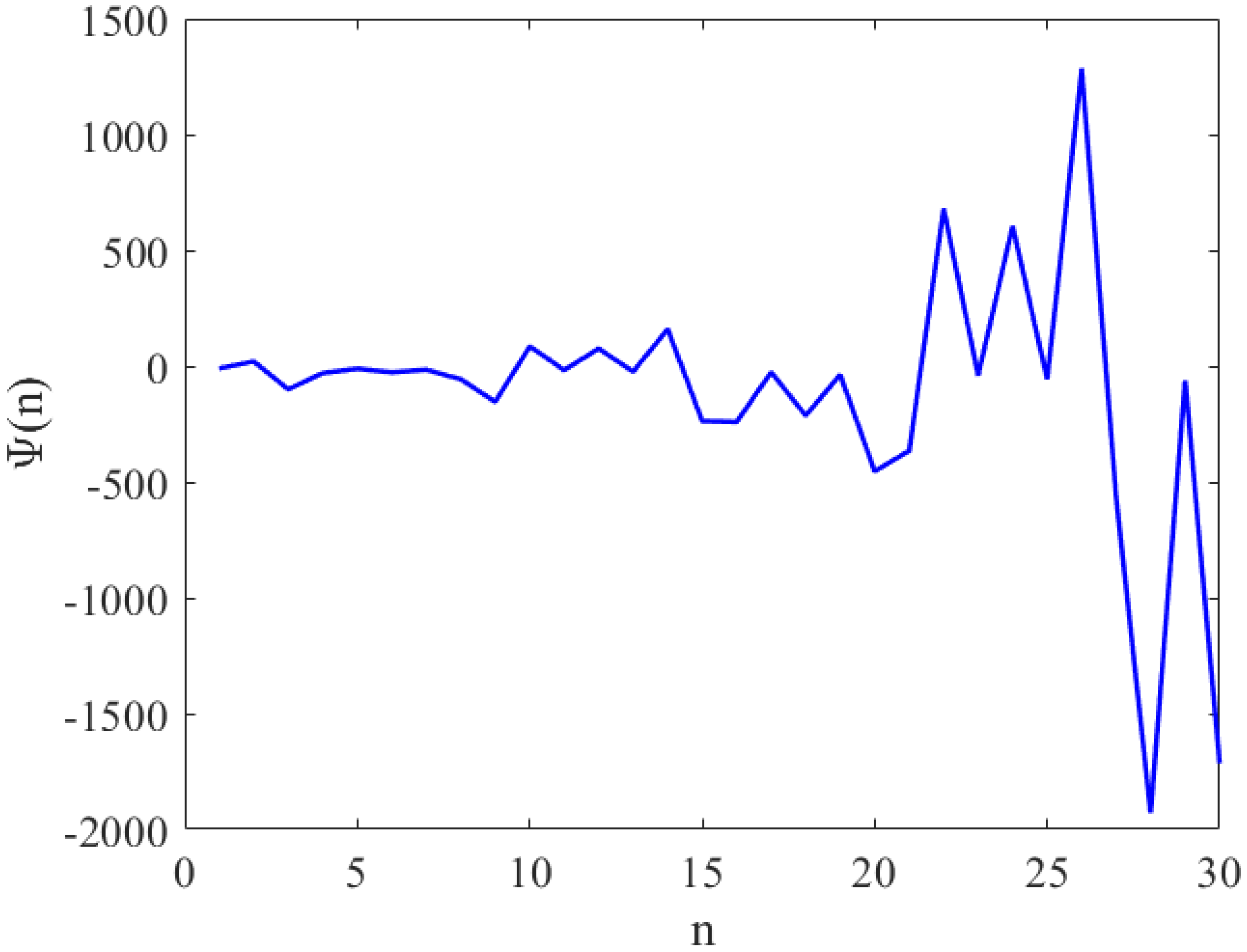
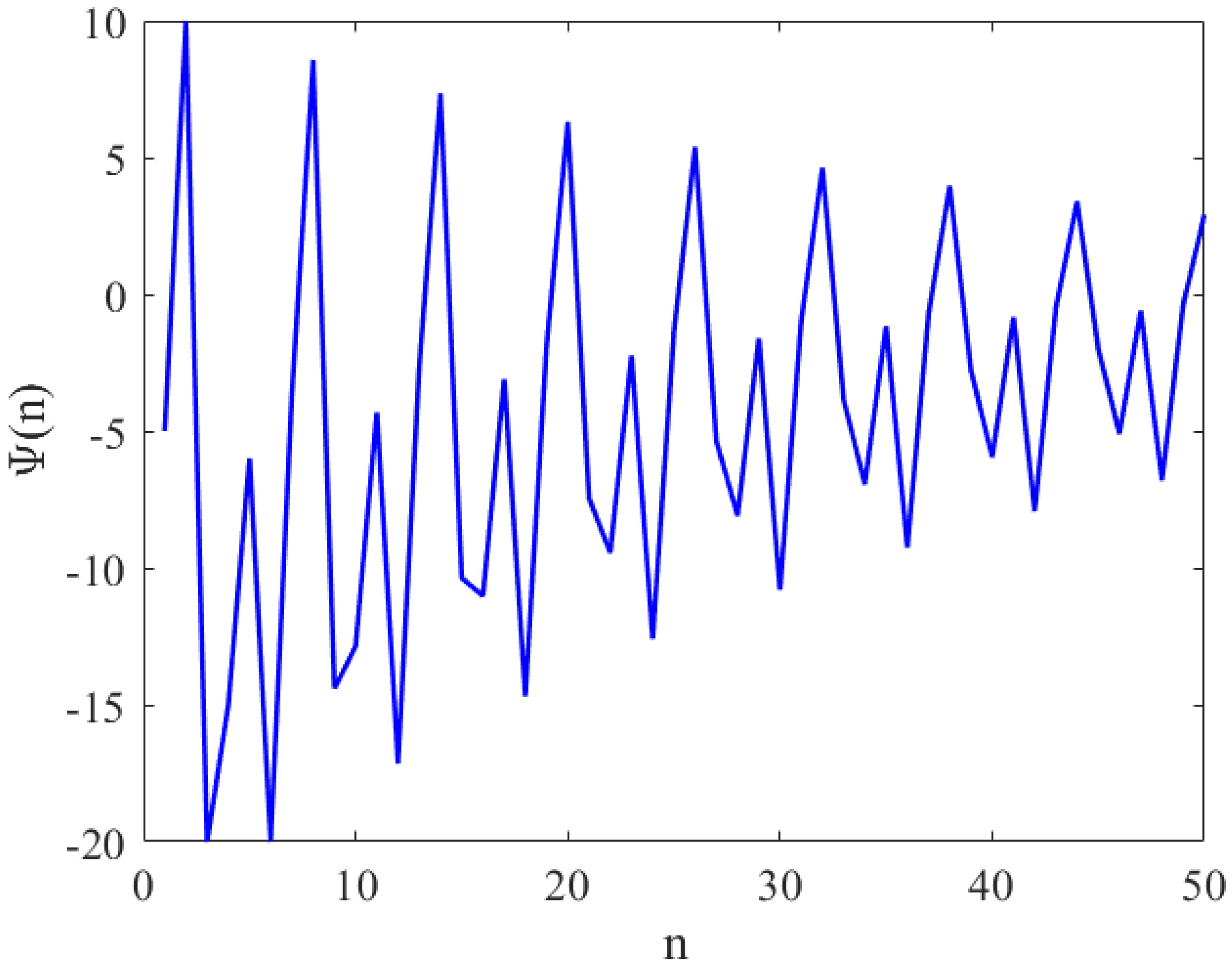
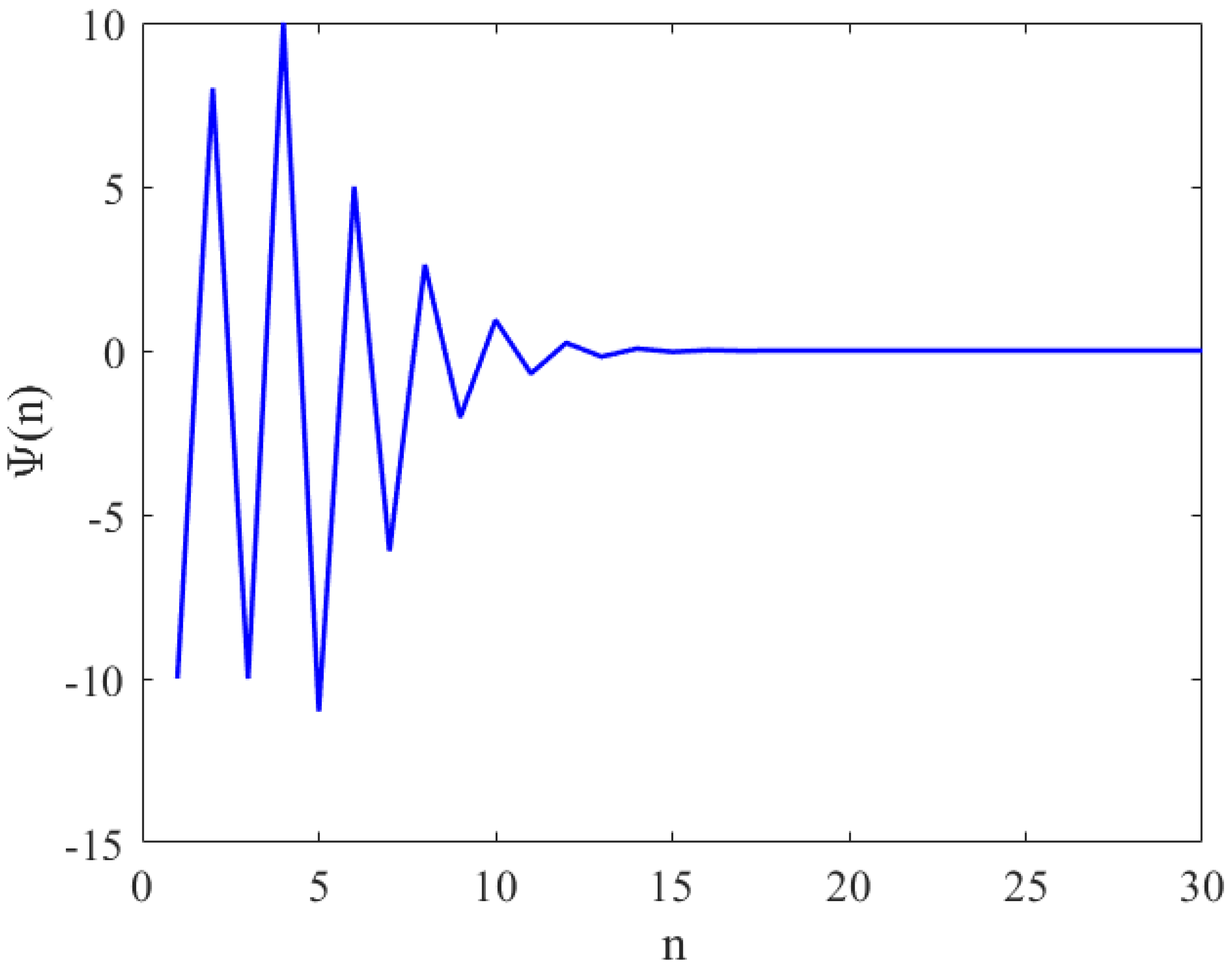
3. Solutions of Some Particular Cases
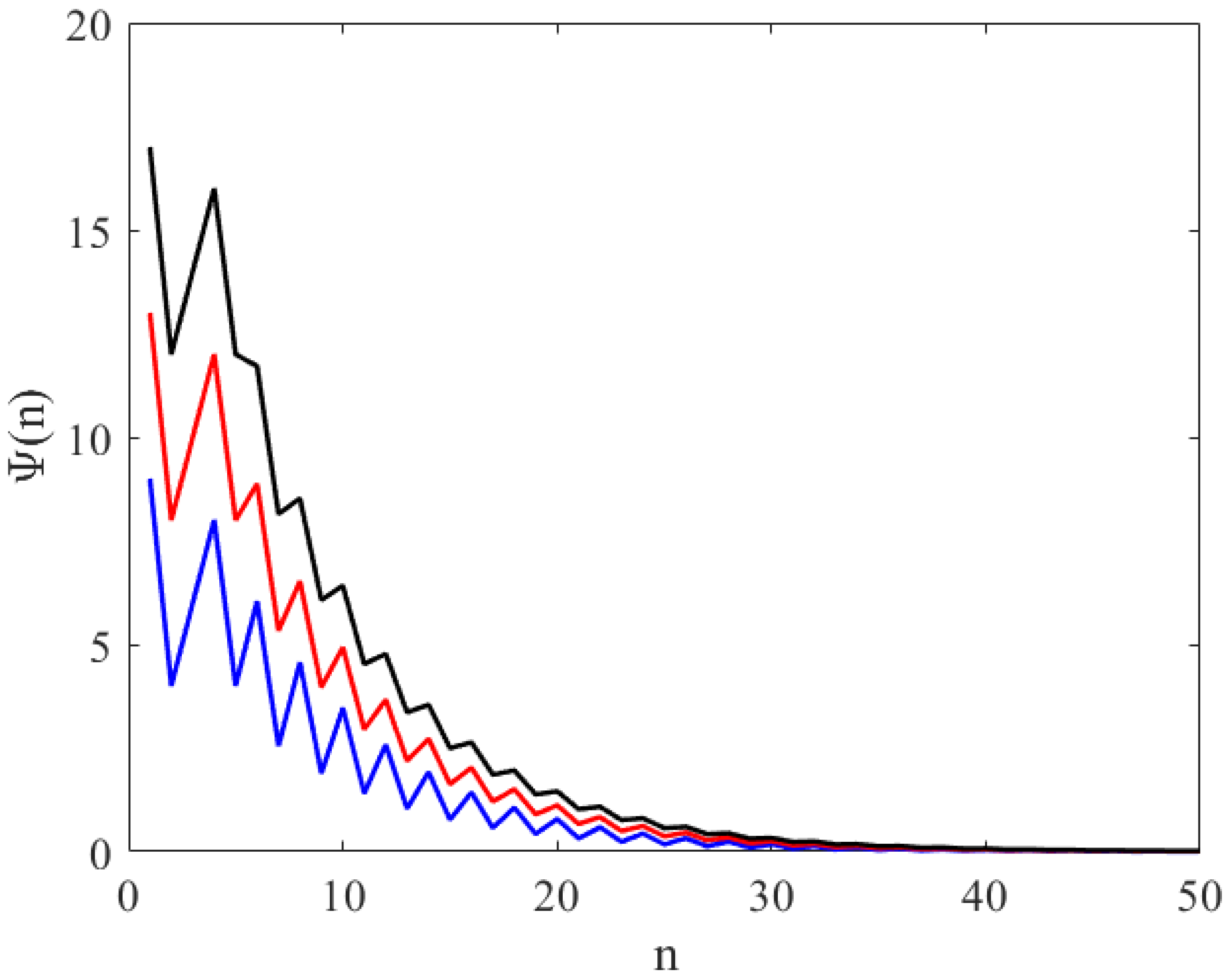
3.1. Case 1:
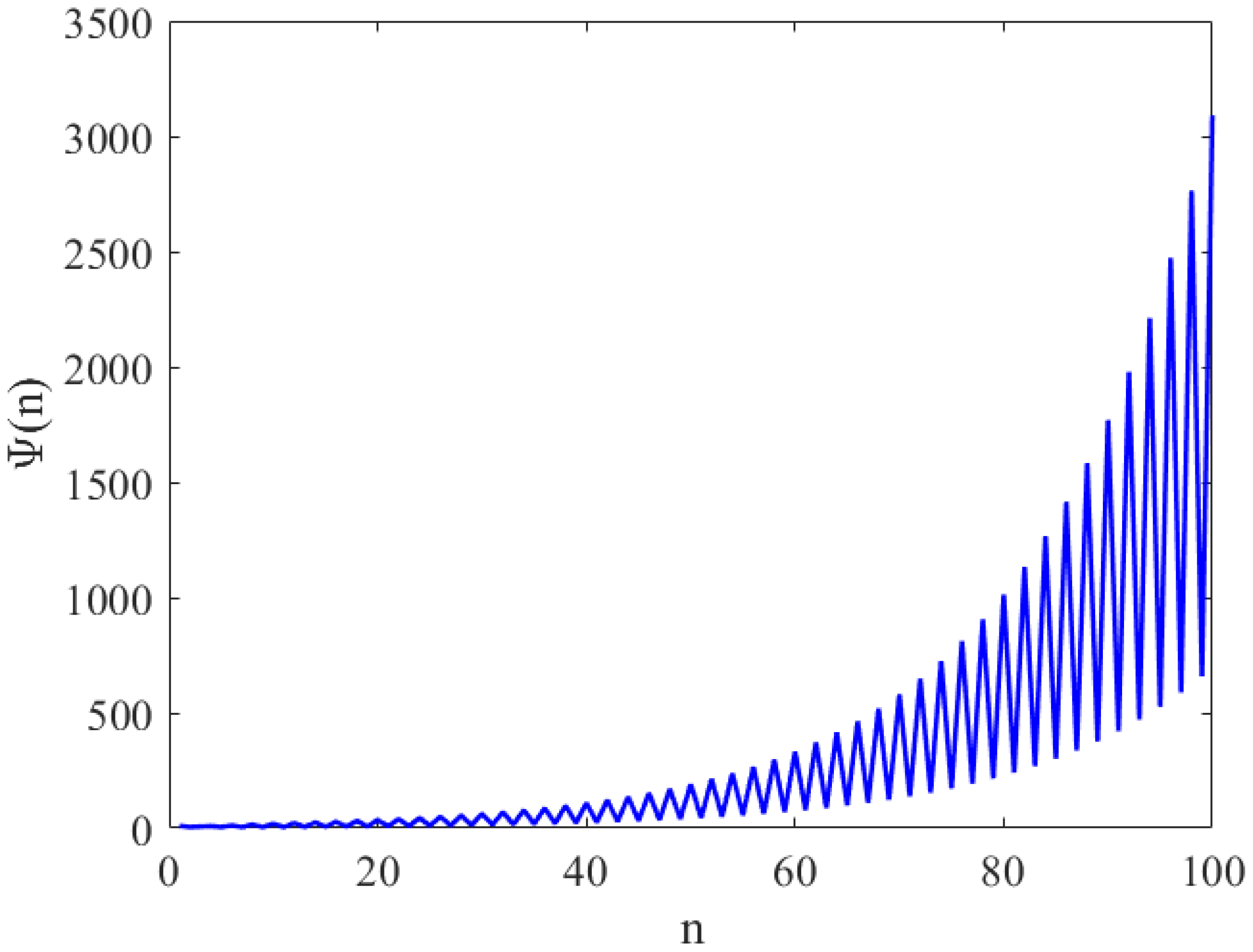
3.2. Case 2:
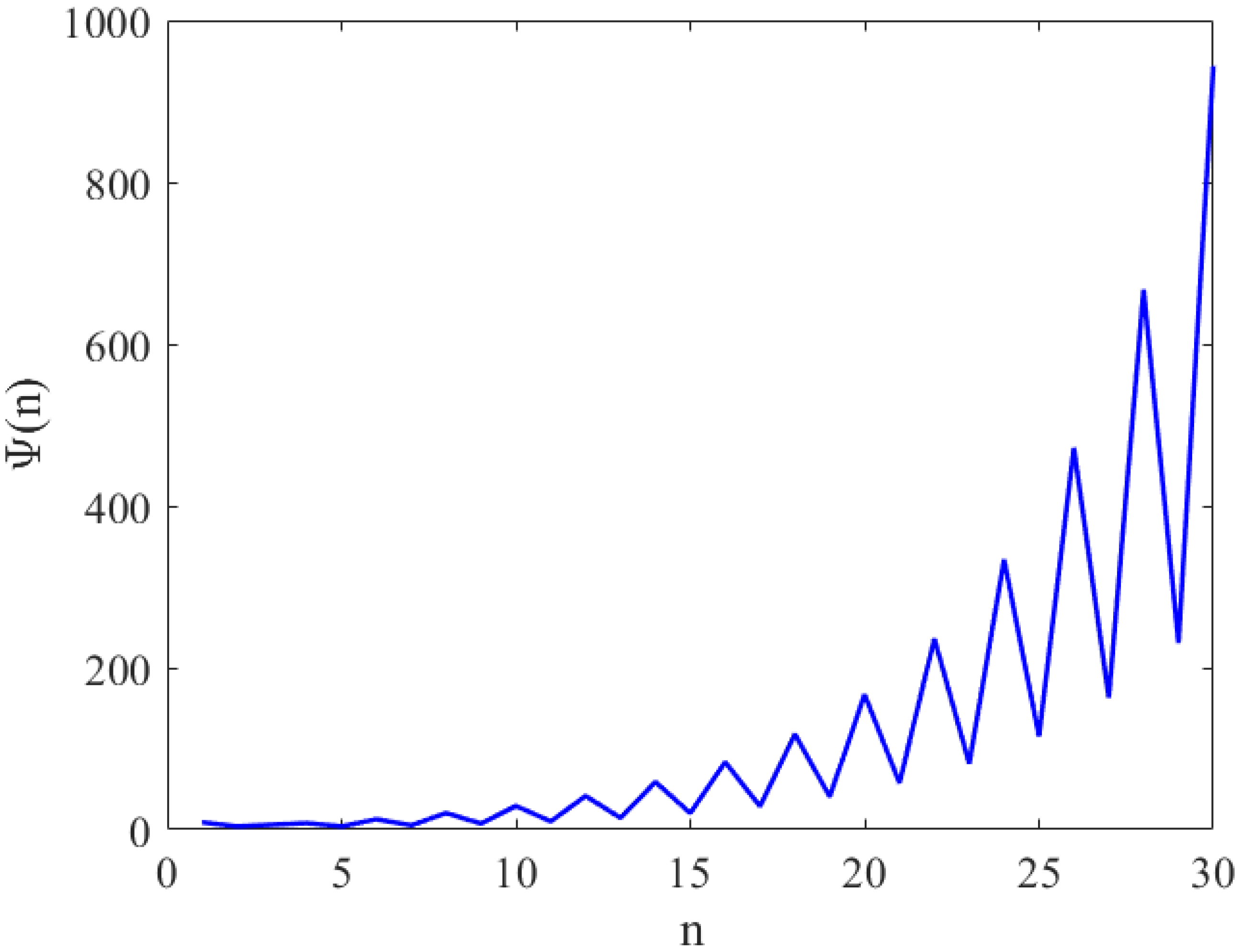
3.3. Case 3:
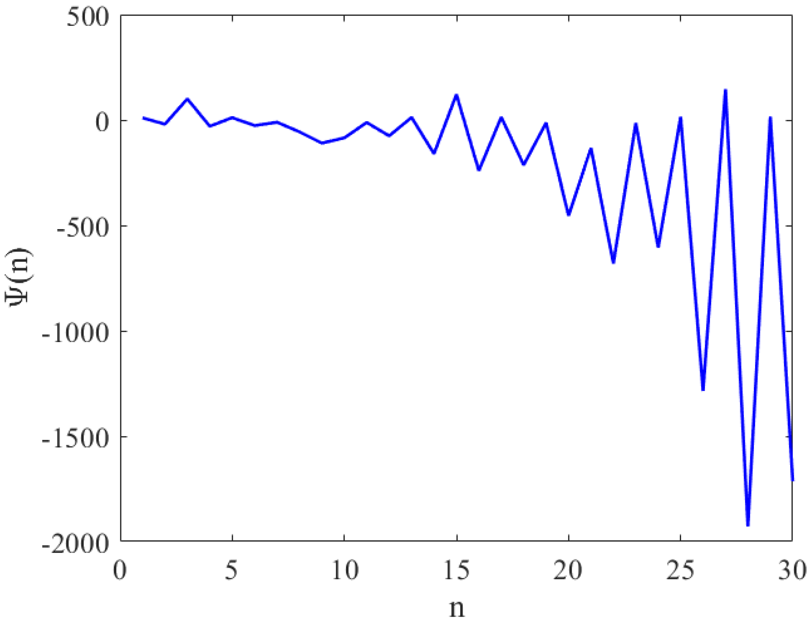
3.4. Case 4:
4. Conclusions
Author Contributions
Funding
Institutional Review Board Statement
Informed Consent Statement
Data Availability Statement
Conflicts of Interest
References
- Cull, P.; Flahive, M.; Robson, R. Difference Equations: From Rabbits to Chaos, Undergraduate Texts in Mathematics; Springer: New York, NY, USA, 2005. [Google Scholar]
- Beverton, R.J.H.; Holt, S.J. On the Dynamics of Exploited Fish Populations. In Fishery Investigations Series II; Blackburn Press: Caldwell, NJ, USA, 2004; Volume 19. [Google Scholar]
- Kuruklis, S.; Ladas, G. Oscillation and global attractivity in a discrete delay logistic model. Quart. Appl. Math. 1992, 50, 227–233. [Google Scholar] [CrossRef] [Green Version]
- Pielou, E.C. An Introduction to Mathematical Ecology; John Wiley & Sons: New York, NY, USA, 1965. [Google Scholar]
- Kocic, V.L.; Ladas, G. Global Behavior of Nonlinear Difference Equations of Higher order with Applications; Kluwer Academic Publishers: Dordrecht, The Netherlands, 1993. [Google Scholar]
- Stevic, S. The recursive sequence ωn+1 = g(ωn, ωn−1)/(A + ωn). Appl. Math. Lett. 2002, 15, 305–308. [Google Scholar]
- Karakostas, G.L.; Stevic, S. On the recursive sequence ωn+1 = α + ωn−k/f(ωn, ωn−1, …, ωn−k+1). Demonstr. Math. 2005, 3, XXXVIII. [Google Scholar]
- Elsayed, E.M.; Alzahrani, F.; Abbas, I.; Alotaibi, N.H. Dynamical behavior and solution of nonlinear difference equation via fibonacci sequence. J. Appl. Anal. Comput. 2020, 10, 281–288. [Google Scholar] [CrossRef]
- Ogul, B.; Simsek, D.; Ibrahim, T. Solution of the Rational differnce Equation, Dynamics of Continuous. Discrete and Impulsive Systems Series. Appl. Algorit. 2021, 28, 125–141. [Google Scholar]
- Ahmed, E.; Hegazi, A.S.; Elgazzar, A.S. On difference equations motivated by modelling the heart. Nonlinear Dyn. 2006, 46, 49–60. [Google Scholar] [CrossRef] [Green Version]
- Chatzarakis, G.E.; Elabbasy, E.M.; Moaaz, O.; Mahjoub, H. Global analysis and the periodic character of a class of difference equations. Axioms 2019, 8, 131. [Google Scholar] [CrossRef] [Green Version]
- Din, Q. Bifurcation analysis and chaos control in discrete-time glycolysis models. J. Math. Chem. 2018, 56, 904–931. [Google Scholar] [CrossRef]
- Elsayed, E.M. New Method to obtain Periodic Solutions of Period Two and Three of a Rational Difference Equation. Nonlinear Dyn. 2015, 79, 241–250. [Google Scholar] [CrossRef]
- Franke, J.E.; Hoag, J.T.; Ladas, G. Global attractivity and convergence to a two-cycle in a difference equation. J. Differ. Eq. Appl. 1999, 5, 203–209. [Google Scholar] [CrossRef]
- Kulenovic, M.R.S.; Ladas, G. Dynamics of Second Order Rational Difference Equations with Open Problems and Conjectures; Chapman & Hall/CRC Press: Boca Raton, FL, USA, 2001. [Google Scholar]
- Moaaz, O. Comment on new method to obtain periodic solutions of period two and three of a rational difference equation. Nonlinear Dyn. 2017, 88, 1043–1049. [Google Scholar] [CrossRef]
- Moaaz, O.; Chalishajar, D.; Bazighifan, O. Some Qualitative Behavior of Solutions of General Class of Difference Equations. Mathematics 2019, 7, 585. [Google Scholar] [CrossRef] [Green Version]
- Moaaz, O.; Chatzarakis, G.E.; Chalishajar, D.; Bazighifan, O. Dynamics of general class of difference equations and population model with two age classes. Mathematics 2020, 8, 516. [Google Scholar] [CrossRef] [Green Version]
- Rasin, O.G.; Hydon, P.E. Symmetries of integrable difference equations on the quad-graph. Stud. Appl. Math. 2007, 119, 253–269. [Google Scholar] [CrossRef]
- Xenitidis, P. Determining the symmetries of difference equations. Proc. R. Soc. A 2018, 474, 20180340. [Google Scholar] [CrossRef] [Green Version]
- Xenitidis, P. Symmetries and conservation laws of the ABS equations and corresponding differential-difference equations of Volterra type. J. Phys. A 2011, 44, 435201. [Google Scholar] [CrossRef] [Green Version]


Publisher’s Note: MDPI stays neutral with regard to jurisdictional claims in published maps and institutional affiliations. |
© 2022 by the authors. Licensee MDPI, Basel, Switzerland. This article is an open access article distributed under the terms and conditions of the Creative Commons Attribution (CC BY) license (https://creativecommons.org/licenses/by/4.0/).
Share and Cite
Elsayed, E.M.; Aloufi, B.S.; Moaaz, O. The Behavior and Structures of Solution of Fifth-Order Rational Recursive Sequence. Symmetry 2022, 14, 641. https://doi.org/10.3390/sym14040641
Elsayed EM, Aloufi BS, Moaaz O. The Behavior and Structures of Solution of Fifth-Order Rational Recursive Sequence. Symmetry. 2022; 14(4):641. https://doi.org/10.3390/sym14040641
Chicago/Turabian StyleElsayed, Elsayed M., Badriah S. Aloufi, and Osama Moaaz. 2022. "The Behavior and Structures of Solution of Fifth-Order Rational Recursive Sequence" Symmetry 14, no. 4: 641. https://doi.org/10.3390/sym14040641