Improved Search for Neutron to Mirror-Neutron Oscillations in the Presence of Mirror Magnetic Fields with a Dedicated Apparatus at the PSI UCN Source

Abstract

While the international nEDM collaboration at the Paul Scherrer Institut (PSI) took data in 2017 that covered a considerable fraction of the parameter space of claimed potential signals of hypothetical neutron (n) to mirror-neutron ($n^{\prime }$) transitions, it could not test all claimed signal regions at various mirror magnetic fields. Therefore, a new study of $n-n^{\prime }$ oscillations using stored ultracold neutrons (UCNs) is underway at PSI, considerably expanding the reach in parameter space of mirror magnetic fields ($B^{\prime }$) and oscillation time constants (${\tau }_{n{n}^{\prime }}$). The new apparatus is designed to test for the anomalous loss of stored ultracold neutrons as a function of an applied magnetic field. The experiment is distinguished from its predecessors by its very large storage vessel (1.47 m³), enhancing its statistical sensitivity. In a test experiment in 2020 we have demonstrated the capabilities of our apparatus. However, the full analysis of our recent data is still pending. Based on already demonstrated performance, we will reach sensitivity to oscillation times ${\tau }_{n{n}^{\prime }}/\sqrt{cos\left(\beta \right)}$ well above a hundred seconds, with $\beta$ being the angle between $B^{\prime }$ and the applied magnetic field B. The scan of B will allow the finding or the comprehensive exclusion of potential signals reported in the analysis of previous experiments and suggested to be consistent with neutron to mirror-neutron oscillations.

1. Motivation

Already in the seminal publication by Lee and Yang on the possibility of the violation of parity symmetry to explain some observed phenomena [1], the authors pointed out the possibility of an additional symmetry, today known as mirror symmetry, which gives rise to the existence of mirror particles.

Parity can be interpreted as a discrete symmetry which exchanges ordinary left-handed particles with their right-handed mirror partners. Kobzarev, Okun and Pomeranchuk [2] observed that mirror particles could not have ordinary strong, weak or electromagnetic interactions, and so they would have to form a hidden parallel sector as an exact duplicate of ordinary matter, with which they interact only via gravity. Thus, all known particles—the electron e, proton p, neutron n, neutrinos $\nu$, etc.— could have mirror partners—$e^{\prime }$, $p^{\prime }$, $n^{\prime }$, ${\nu }^{\prime }$—with exactly the same masses, being sterile to known strong and electroweak interactions, but having their own interactions with each other, in the same ways as their Standard Model partners. This idea was applied as an extension to the Standard Model in [3] and worked on by various authors over the decades (for a review, see, e.g., [4,5,6]; for a historical overview, see also [7]).

These thoughts have received renewed interest over the past 20 years, as it was shown that mirror matter could provide viable candidates for the dark matter in the Universe [8,9,10] (more extended discussions of its properties can be found in reviews [4,5,6]). The interest further increased because of the absence of other clear signals of dark matter particles and the ability to explain a number of difficulties in collisionless cold dark matter models. Since mirror matter is atomic/dissipative dark matter it can form dark stars and other compact objects [8,11,12,13].

Plausible cross-interactions between mirror and ordinary particles, induced, e.g., by the photon-mirror-photon kinetic mixing [14,15] would, in spite of severe cosmological [16] and experimental [17] limits, provide an efficient mechanism for inducing a galactic magnetic field [18]. They could be revealed via direct detection in dark matter detectors [19,20,21]. In addition, ordinary and mirror sectors can have common gauge interactions related to flavor symmetry [22,23,24] and $B-L$ symmetry [25,26], or common Peccei-Quinn symmetry [27,28]. A distinct feature of this concept is that some of these cross-interactions may violate baryon (and/or lepton) numbers of both ordinary and mirror sectors. At first, these interactions, satisfying Sakharov’s conditions [29], can give rise to co-baryogenesis (or co-leptogenesis) mechanisms in the early Universe, which can be the origin of baryon asymmetries in both sectors [30,31]. They also could explain the observed cosmological fractions of visible and dark matter components in the Universe [32,33]. Secondly, these interactions can induce oscillation phenomena between ordinary and mirror particles. In fact, any neutral particle, elementary (e.g., neutrinos) or composite (e.g., neutrons), can have a mixing with its mass degenerate mirror partner and thus can oscillate into the latter. In particular, “active-sterile” mixings between three ordinary neutrinos ${\nu }_{e\mu \tau }$ and three mirror neutrinos ${\nu }_{e\mu \tau }^{\prime }$ were discussed in [34,35,36].

The possibility of the neutron mass mixing with the mirror neutron was proposed in [37]. The phenomenon of $n-n^{\prime }$ oscillation is similar to the neutron–antineutron oscillation $n-\overline{n}$ (see [38] for a review). Both phenomena of $n-n^{\prime }$ and $n-\overline{n}$ mixing might originate from the same mechanism in the context of theoretical models [37]. However, there are many substantial differences:

• $n-\overline{n}$ mixing violates baryon number by two units ($\mathsf{\Delta }\mathrm{B}=2$) whereas $n-n^{\prime }$ mixing violates it by one unit ($\mathsf{\Delta }\mathrm{B}=1$);
• The mass degeneracy between the neutron and antineutron stems from CPT invariance. Between the neutron and mirror neutron it is a consequence of mirror parity which in principle can be spontaneously broken;
• Existing limits on the characteristic $n-\overline{n}$ oscillation time are rather stringent. Namely, the experimental direct limit on the $n-\overline{n}$ oscillation time is ${\tau }_{n\overline{n}}>0.86\times {10}^8$ s [39]. Indirect limits from nuclear stability are even stronger, ${\tau }_{n\overline{n}}>2.7\times {10}^8$ s [40]. As for $n-n^{\prime }$ oscillation, its characteristic time ${\tau }_{n{n}^{\prime }}$ can be as low as a few seconds, and in any case much smaller than the neutron lifetime, without contradicting either existing astrophysical and cosmological limits or, unlike $n-\overline{n}$ oscillations, nuclear stability limits [37]. The reason why such fast $n-n^{\prime }$ oscillations are not directly manifested experimentally in the neutron losses, is that in normal conditions it is suppressed by environmental factors as the presence of matter and/or magnetic fields [37,41].

Moreover, such fast $n-n^{\prime }$ oscillations can have interesting and testable implications for ultra-high-energy cosmic rays [42,43], for the neutrons from solar flares [44], for neutron stars [45,46,47], for primordial nucleosynthesis [48], and can also potentially explain the neutron lifetime anomaly [49,50]. In addition, it requires the existence of BSM physics off the beaten track, e.g., color scalar particles, at the scale of a few TeV, which can be tested at the LHC and future accelerators [37,51]. In a more general picture, the neutron n can have mixings with both the mirror neutron $n^{\prime }$ and mirror antineutron ${\overline{n}}^{\prime }$, with respective masses ${ϵ}_{n{n}^{\prime }}$ and ${ϵ}_{n{\overline{n}}^{\prime }}$ which in combination can induce neutron–antineutron oscillation at the second order via the oscillation chain $n\to n^{\prime },{\overline{n}}^{\prime }\to \overline{n}$, with a characteristic timescale ${\left({\tau }_{n{n}^{\prime }}{\tau }_{n{\overline{n}}^{\prime }}\right)}^{1/2}$ which can be much shorter than the direct $n-\overline{n}$ oscillation time ${\tau }_{n\overline{n}}$ [52].

In 2006 it was pointed out that direct experimental limits on $n-n^{\prime }$ oscillations virtually did not exist [37], indicating the possibility of an oscillation time ${\tau }_{n{n}^{\prime }}$ as short as 1 s. It was suggested to search for these oscillations in laboratories via the neutron disappearance $n\to n^{\prime }$ or regeneration $n\to n^{\prime }\to n$ (see also [53,54]).

Previous Experimental Efforts

Since then, several experimental collaborations embarked on measurements in search of $n-n^{\prime }$ oscillations, mostly looking for signals of neutron disappearance in storage experiments with ultracold neutrons (UCNs). Most prominently, two collaborations equipped with setups to search for the neutron electric dipole moment provided the relevant limits. The first experimental limit ${\tau }_{n{n}^{\prime }}>103$ s (95% C.L.) [55] was obtained at ILL by the nEDM collaboration that is today working at PSI and has considerable overlap with the authors of the present study. The strongest experimental limit ${\tau }_{n{n}^{\prime }}>414$ s (95% C.L.) was obtained at ILL by the collaboration centered around the PNPI team of A. Serebrov [56]. These results were obtained by assuming, as in the original paper [37], that there are no effects of mirror matter at the Earth which could affect $n-n^{\prime }$ oscillations. Therefore, these experiments compared the UCN losses in conditions of vanishing ($B\ll 10$ nT) and large enough ($B>1$ μT) magnetic fields. These thus assumed that n and $n^{\prime }$ would be degenerate around $B=0$ while the application of a magnetic field B of a few μT would already lift the degeneracy and effectively suppress potential oscillations.

Mirror magnetic fields can be induced by a rather tiny amount of mirror matter [9] which can be captured by the Earth, due to the mirror electron drag mechanism which the Earth rotation may cause. The mirror magnetic field can reach values comparable to the normal magnetic field of the Earth, up to hundreds of μT. In the case of non-zero $B^{\prime }$, $n-n^{\prime }$ oscillation at $B\approx 0$ will be suppressed, but it would be resonantly enhanced if $B\approx B^{\prime }$. Therefore, for finding $n-n^{\prime }$ oscillation effects, the value of the applied magnetic field should closely match the unknown value of $B^{\prime }$.

Unlike the normal magnetic field, the mirror field cannot be screened in experiments, and its direction is also unknown. As was suggested in [41], these effects can be searched for by measuring UCN losses at different values of the applied field B. Then, one can measure the directional asymmetry $A_{\uparrow \downarrow }$ by comparing the UCN counts between cycles with opposite directions of the applied field at the given value ($+B$ and $-B$).

$$A_{\uparrow \downarrow }=\frac{n_{\uparrow }-n_{\downarrow }}{n_{\uparrow }+n_{\downarrow }},$$

(1)

where $n_{\uparrow ,\downarrow }$ represents the UCN counts $N_{\uparrow ,\downarrow }$ after a UCN storage time $t_s$, normalized with the corresponding monitor counts $M_{\uparrow ,\downarrow }$ (see Section 2.1). The value of $A_{\uparrow \downarrow }$ should depend on the absolute value of $B^{\prime }$ as well as on the angle $\beta$ between the ordinary and mirror fields.

Following [41] we can then derive the oscillation time

$${\tau }_{n{n}^{\prime }}(B,B^{\prime })=\sqrt{\frac{t_{\mathrm{s}}}{\langle t_{\mathrm{f}}\rangle A_{\uparrow \downarrow }}}\sqrt{f_A(B,B^{\prime })\cos \beta },$$

(2)

where $\langle t_{\mathrm{f}}\rangle$ is the average value of the mean free flight time of the UCN during storage, $f_A(B,B^{\prime })$ a simple function of B and $B^{\prime }$ [57], $\beta$ the angle between the vectors B and $B^{\prime }$. Obviously, in the absence of an effect, the asymmetry would be zero and a limit on ${\tau }_{n{n}^{\prime }}$ can be derived, albeit in combination with the dependence on the angle $\beta$ between B and $B^{\prime }$.

Moreover, a ratio E can be measured, by comparing the UCN counts averaged between $+B$ and $-B$ cycles with the counts $n_0$ measured at $B=0$, with

$$E\equiv \frac{2n_0}{n_{\uparrow }+n_{\downarrow }}-1=\frac{t_s}{\langle t_f\rangle }\frac{1}{{\tau }_{n{n}^{\prime }}^2}{f}_E(B,B^{\prime })$$

(3)

with $f_E(B,B^{\prime })$ is another simple function of B and $B^{\prime }$ [57], but different from $f_A$.

The latter ratio should not depend on the unknown direction of the mirror field but only on its absolute value. Namely, by measuring the values of E and A consistent with zero at different applied fields B, one sets the limits on respectively ${\tau }_{n{n}^{\prime }}$ and ${\tau }_{n{n}^{\prime }}/\sqrt{cos\beta }$ for a given inferred value of $B^{\prime }$. In a more general case when both $n-n^{\prime }$ and $n-{\overline{n}}^{\prime }$ oscillations are present, e.g., E-measurements would restrict an effective combination ${\tau }_{\mathrm{eff}}={({ϵ}_{n{n}^{\prime }}^2+{ϵ}_{n{\overline{n}}^{\prime }}^2)}^{1/2}$ [52], and thus restrict ${\tau }_{n{n}^{\prime }}$ and ${\tau }_{n{\overline{n}}^{\prime }}$.

As the possibility of non-zero $B^{\prime }$ came into focus, experiments quickly measured E and A at different values of B excluding also a sizeable fraction of the parameter space with non-vanishing $B^{\prime }$ fields [54,57,58,59,60]. However, some measurements have shown deviations from the null hypothesis. In particular, reanalysis of the data of the experiment [59] in [61] revealed signal-like effects at the $5\sigma$ level. The original study [59] reports a $3\sigma$ deviation from zero for the A-asymmetry after averaging between measurements at different values of B, which is problematic once the $n-n^{\prime }$ oscillation probability is supposed to have a resonant dependence on $B^{\prime }$ [41]. In addition, the data of experiment [62] have shown a $2.5\sigma$ deviation, again for the A-asymmetry.

Using the nEDM spectrometer, the nEDM collaboration at PSI performed a $n-n^{\prime }$ search in 2017, which was designed to test the deviations and allowed signal regions claimed in [61]. The exclusion plot shown in Figure 1 summarizes the status of $n-n^{\prime }$ experimental results from the asymmetry channel. The claimed potential signals of [61] are excluded by the 2017 data of the nEDM collaboration analyzed in the context of a PhD thesis [63] and recently published [57]. However, further reanalysis [62] of the magnetic field conditions of the experiment [59] resulted in a wider range of possible signal regions indicated by the signal bands in the figure. These new potential signal regions were only partially excluded, as this information was not yet available at the time of planning and data taking in 2017.

A recent experiment at the SNS, Oakridge National Laboratory [64] performed at $B\simeq 4.8$ T, excluded a parameter space of neutron–mirror-neutron mixing for $n-n^{\prime }$ mass splittings in the range $\mathsf{\Delta }m=50–400$ neV. However, this experiment was not sensitive for smaller $\mathsf{\Delta }m$. In contrast, our experiment is sensitive for a range of $\mathsf{\Delta }m<0.1$ neV, and in particular in the case when n and $n^{\prime }$ are degenerate in mass.

2. Experiment

We present in this work a novel experiment designed to probe the entire relevant parameter space, and to confirm or refute the claimed mirror neutron signals compatible with previous results. In 2020, the first version of the apparatus was used in a short beam time to demonstrate its performance at the West-1 beamport of the ultracold neutron source at PSI [65,66,67,68,69,70]. In spring 2021, several aspects of the apparatus were improved in preparation for the main data-taking run.

2.1. Concept

The concept of this experiment is based on the search for increased losses of ultracold neutrons during storage, in resonance with a vertical magnetic field at specific field values. In our measurements, the number of UCNs after storage are normalized to the initial UCN density. If there would be neutron to mirror-neutron oscillations during storage enhanced in resonance either at $+B$ or $-B$, the asymmetry $A_{\uparrow \downarrow }$ (see Equation (1)) would be different from zero.

Our experiment allows two modes of operation, storage and leakage mode.

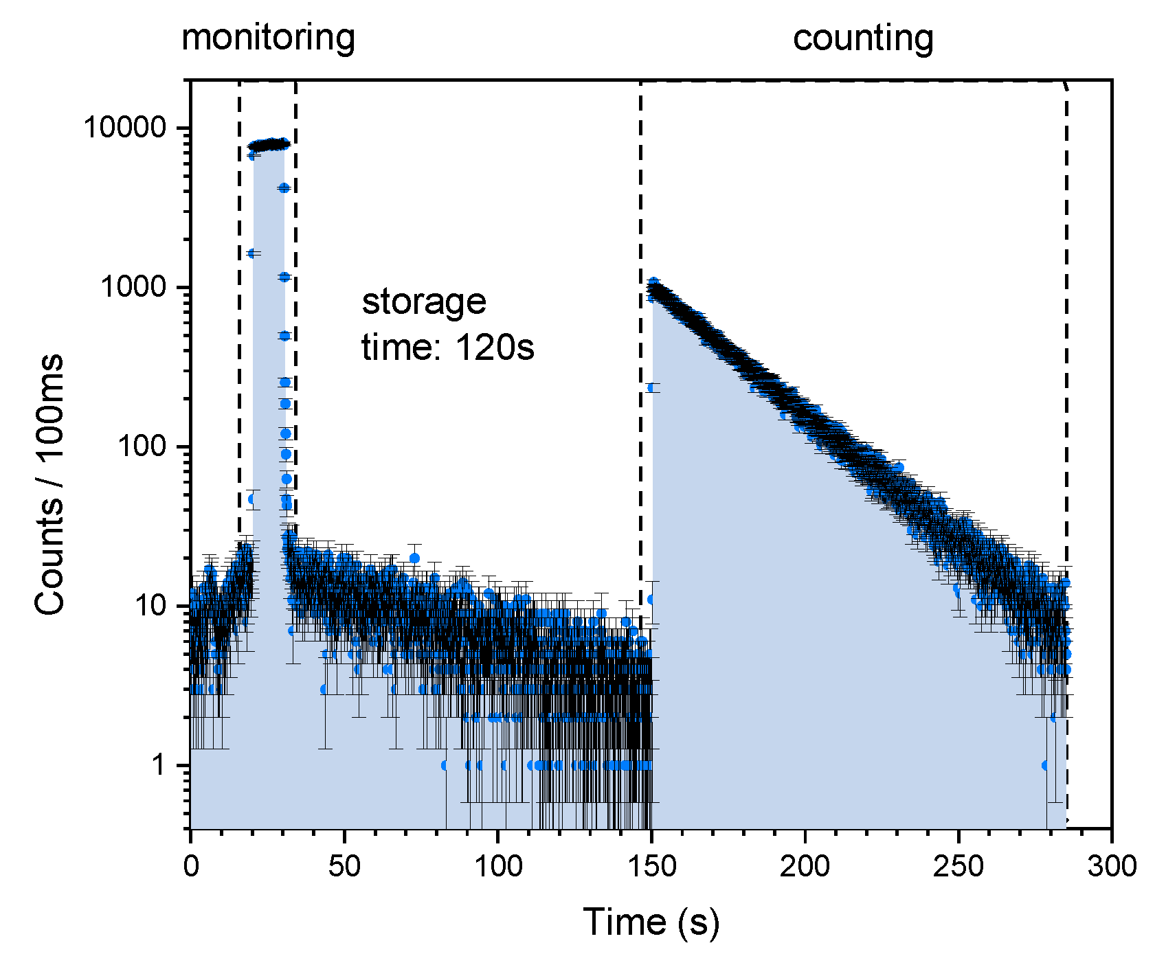
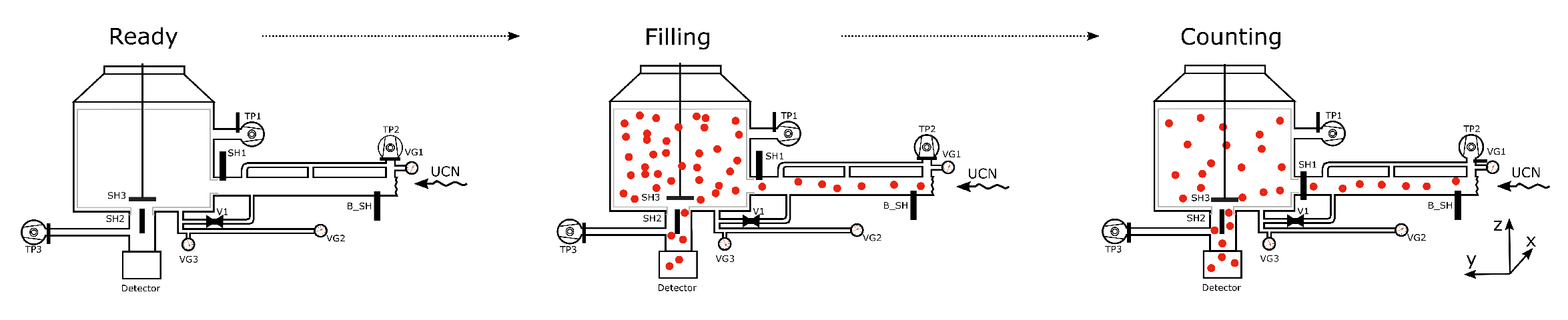
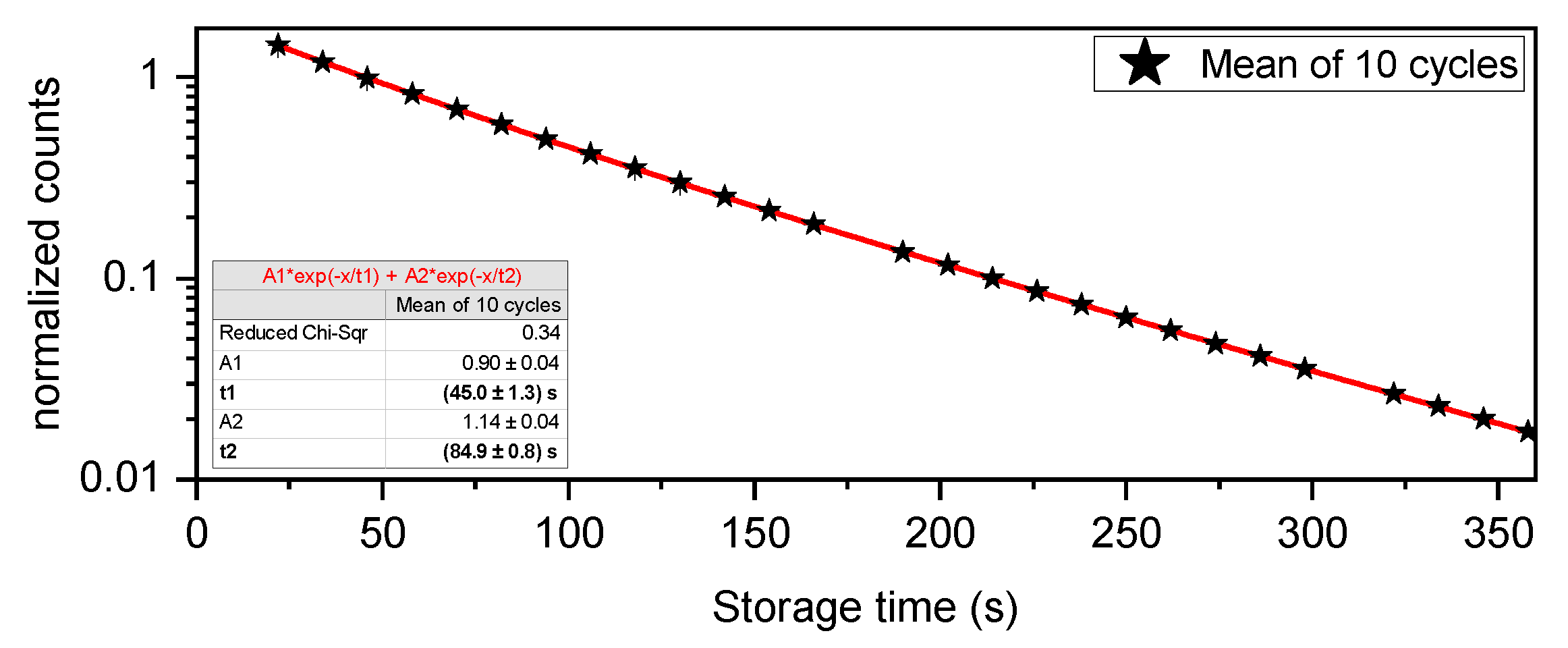
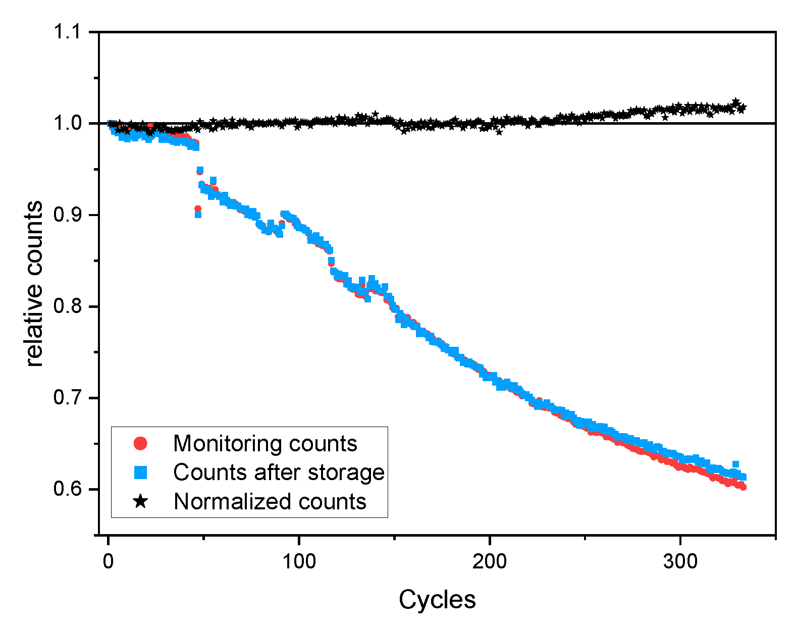
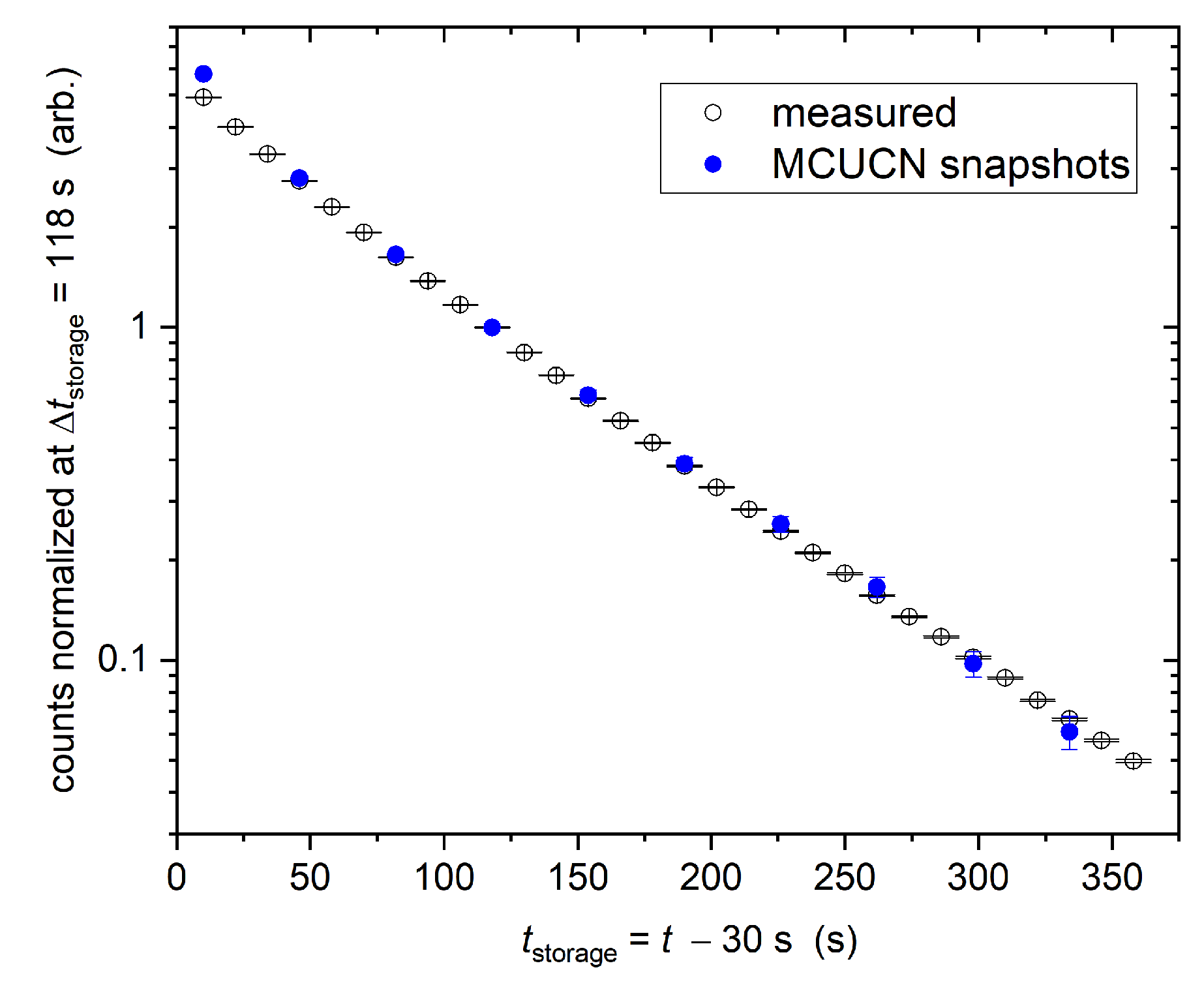
• Classical storage measurement (sketched in Figure 2): UCNs are filled into a storage volume. To measure the initial UCN density, the shutter to the detector SH2 is opened for the last 10 s of the filling (“monitoring”) then closed. The filling shutter SH1 is closed, and UCNs are stored for a given storage time. Then, the second shutter SH2 opens and UCNs are emptied and counted in a detector (“counting”). The time spectrum of UCNs arriving in the detector during such a typical cycle is shown in Figure 3.
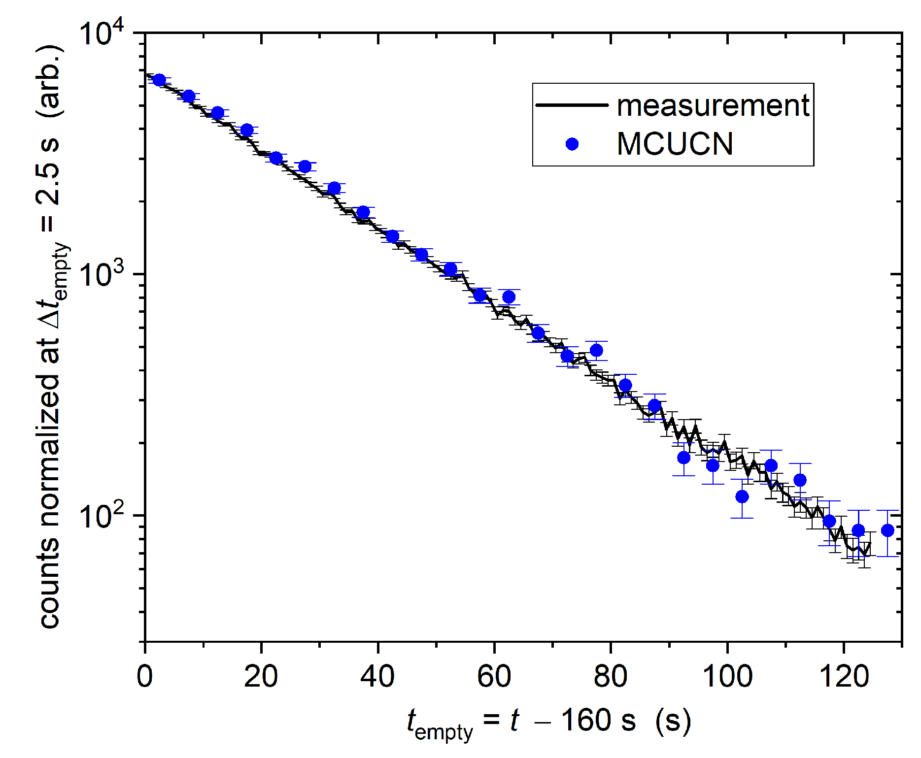
• Leakage measurement (sketched in Figure 4): UCNs are filled into the storage volume and the filling shutter SH1 is closed, but SH2 and hence the storage volume towards the detector are permanently open. An additional shutter suspended from the top (a modification of SH3 which reaches to the bottom of the storage vessel) allows to have a small, adjustable opening to the detector. Hence UCNs are counted continuously. The measured UCN rate at the detector during such a cycle is illustrated in Figure 5. In this scheme the experiment is not only sensitive to variations in total counts but also to the change of the leakage time spectrum.

2.2. Ultracold Neutron System

The setup of the experiment can be explained following the cut-view CAD drawing shown in Figure 6 as used for the fall 2020 measurements. UCNs are guided over 2750 mm from the West-1 beamport shutter to the entrance shutter of the storage vessel using nickel-molybdenum (NiMo)-coated glass guides [65,71,72] with an inside diameter of 130 mm. The 1.47 m³ large UCN storage volume placed inside a large vacuum vessel is made of non-magnetic stainless steel and extends via 200 mm-diameter stainless steel tubes to two shutters. The filling shutter SH1 is a VAT product as described in Ref. [72]. It is coated with diamond-like carbon and is vacuum tight. The emptying shutter is from the standard bottle setup [73] and made from stainless steel. It has a small (∼1%) UCN leakage, but opens and closes fast and reproducibly. The top of the volume has a 200 mm diameter hole which can be opened during pumping periods to increase pumping efficiency. It is closed during UCN storage, otherwise a large fraction of UCNs is lost. The vacuum vessel is made from stainless steel and all parts of the vessel were checked for possible magnetic contamination and replaced where possible.

The detector, a Cascade UCN detector (CDT Cascade Detector Technologies, 69123 Heidelberg, Germany, http://www.cd-t.com) with a sensitive area of 20 cm × 20 cm is located below the emptying shutter and connected via a short stainless-steel guide section which can be evacuated via a 5 mm opening.

The magnetic field is generated via a 3-dimensional coil system as described and first used in [74]. The photo in Figure 7 shows the setup as it was installed and used for the test measurements in fall 2020 in UCN area West-1.

2.3. Improvements of the Ultracold Neutron System in 2021

During the measurements in fall 2020 we have identified various parts of the UCN system which could be slightly upgraded to improve the performance. These modifications will increase the UCN statistics and the UCN storage time constant. Each of these changes has been found to substantially improve the achievable statistical sensitivity in simulations (see Section 3.2).

Some modifications were already implemented and tested:

• In order to increase the UCN storage properties of the storage volume, the entire stainless-steel body of the vessel was electro-polished. This increased the storage time constant as the entire surface and especially the welding seams became cleaner;
• The UCN guide on the bottom of the storage vessel towards the detector is made from stainless steel with a Fermi potential $V_F$ = 185 neV. Coating of the surface with a material of higher $V_F$, namely NiMo with a $V_F$ = 220 neV [72] was applied in order to further reduce wall losses in this region;
• New UCN guides from the beamport to the storage vessel, with a ID = 180 mm NiMo-coated glass guides and a ID = 200 mm polished stainless-steel guide, effectively doubled the cross-section of the guides, however, with the drawback of the metal guide part having a larger surface roughness than glass. Still, this resulted in an increase in the UCN filling rate;
• A new plate shutter (a dynamic version of SH3, shown in Figure 4, that would open and close the storage volume to the detector) was designed and tested. At the same time the shutter SH2 of the standard bottle used in 2020 was coated with NiMo and found to be superior;
• With our UCN simulation tuned to the further detailed measurements, we re-investigate changing the height of the storage vessel with respect to the beamport.

2.4. Magnetic Field System

To compensate ambient magnetic fields and to produce the desired field for the experiment, a set of rectangular coil pairs were erected around the experiment (see Figure 6 and Figure 7), with the neutron storage chamber approximately at the center. The coil system described in [74] has been recommissioned. It has nominal dimensions of 3 m × 3 m × 4.6 m. In the x and z directions, the field is produced by pairs of 3 m × 4.6 m rectangular coils, separated by around 1.8 m. In the y direction, a set of four square 3 m × 3 m coils are located at $y=\pm 0.9$ m and $y=\pm 2.2$ m, with the central coils having four times as many turns as the outer coils. Additionally, the current of each coil can be individually controlled, allowing an adjustment of field gradients.

The homogeneity H(B) of the magnetic field produced by the $B_z$ coil was computed over the neutron storage volume based on the Biot–Savart law, using

$$H\left(B\right)=(B_z^i-B_z^{mean})/B_z^{mean}$$

(4)

with $B_z^i$ the magnetic field computed at several positions covering the UCN storage vessel, and their mean value $B_z^{mean}$. The standard deviation $B_z^i-B_z^{mean}$ is illustrated in Figure 8. The resulting H(B) < 0.5% is considered to be good enough that it does not limit the quality of the field within the chamber. This is ultimately limited by local field inhomogeneities and environmental fields, such as those produced by vacuum pumps and other components critical to the experiment, and those produced by the large steel-armed concrete blocks forming the floor and the walls of the experimental area. To minimize local inhomogeneities, magnetic components such as certain vacuum gauges and pumps were all moved with extension tubes outside the coil cage for the main run in 2021.

Many sources of magnetic field disturbances from other installations surrounding UCN Area West are known from the nEDM measurements in UCN Area South [75]. In particular a large nearby superconducting magnet is known to produce changes in the magnetic field in the order of 100 μT when it is ramped.

During the measurement, an active compensation of the ambient magnetic field was applied. In 2020, a set of 13 Stefan Mayer FLC3-70 three-axis fluxgates was located in the vicinity of the vacuum tank. The locations were chosen to be able to optimally calculate the magnetic field in the storage tank and at the same time to minimize the impact of possible local magnetic field sources such as vacuum pumps. The range of ±200 μT of the sensors set the maximum mirror field that could be probed in 2020. The improved setup in 2021 includes 10 3-axis Sensys FGM3D/125 fluxgates to cover the field range up to 125 μT with a higher accuracy, 5 3-axis Stefan Mayer FLC3-70 fluxgates for a consistency check with the previous year, and 1 higher-range Sensys FGM3D/1000 sensor to allow us to probe even higher fields, limited only to about ±380 μT by the maximum current of the power supplies of the coils. The fluxgates are read out at 50 Hz by a computer-based data-acquisition (DAQ) system fully integrated into the main DAQ system (discussed in full in Section 2.6).

The coils are powered by six computer-controlled DC power supplies each capable of supplying 10/20 A at 35 V, with the possibility to reverse the polarity provided by a system of relays. Two algorithms have been implemented for the control of the coil currents:

• Dynamic: the currents in each coil are set according to a modified version of the “dynamic” algorithm described in [75], aiming to match the readings of each of the first 10 fluxgates to the goal field using a PI feedback algorithm;
• Static: the currents in each coil are set to values to achieve the desired fields based on offline measurements, assuming the external field remains constant.

When it is known that the external field may change, it is mandatory to use the dynamic mode. The coil current is updated at 10 Hz. This is more than enough to allow dynamic compensation of external field changes on the relevant timescale (namely, the average field change over the entire storage time), and even to allow the goal field to be changed during a live measurement. This allows simplification of the analysis by permitting the detuning of the magnetic field during the filling of the neutron storage vessel.

Based on the measured fields in each of the fluxgates, a first estimate was that the actual field homogeneity achieved is better than 3 μT at a field setting of 10 to 20 μT. This is likely an overestimate, as the fluxgates are located outside the chamber and therefore influenced by ambient magnetic field sources.

The effect of field inhomogeneity is a slight broadening of the range of mirror fields probed by each run, as effectively multiple field values are probed simultaneously. Our experiment is not targeting the $B^{\prime }=0$ region and therefore does not require zero field capability on a level below a few μT. Better knowledge of the magnetic field was acquired during a dedicated mapping campaign before the 2021 measurement period (see Section 2.5) with the full analysis not yet finished.

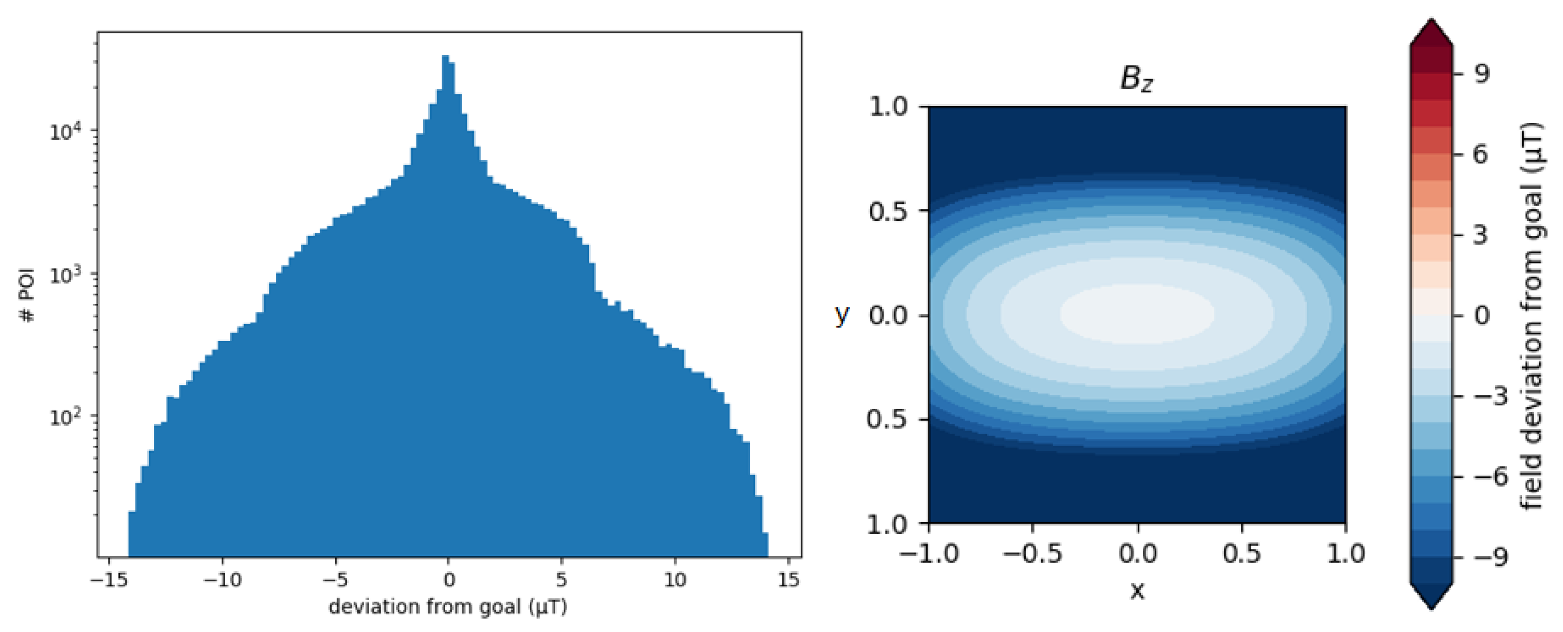
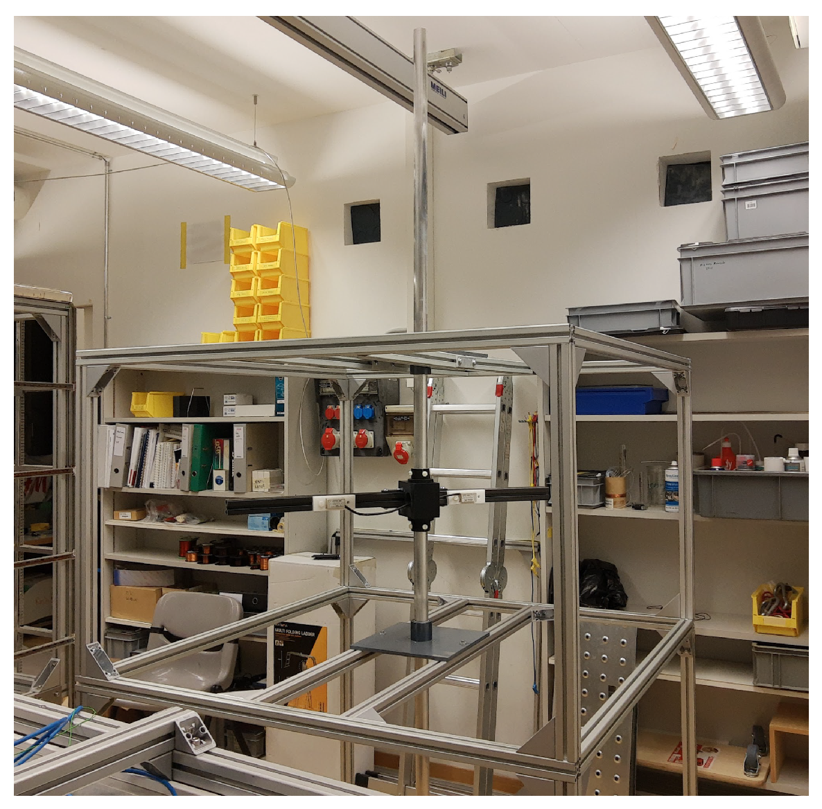
2.5. Mapping of the Magnetic Field

For the interpretation of the neutron storage measurements in terms of a mirror neutron signal, it is important to quantify the field distribution within the neutron storage chamber during measurement. During neutron data-taking in 2020, a set of 13 three-axis fluxgate magnetometers monitored the field in the vicinity of the storage chamber (see Section 2.4). However, after all magnetic apparatus components were moved outside the coil cage, the remaining ambient field in the proximity of the storage chamber due to non-removable parts of the apparatus, i.e., magnetized welding seams on flanges or on the floor of the vacuum tank, and the nearby armed concrete shielding, makes a simple interpolation or fitting difficult.

A mapper device was designed and prototyped, inspired by the mappers used by the nEDM and n2EDM experiments [76,77], with substantial simplifications. A vertical axle passes through bearings mounted on flanges on the top and bottom of the vacuum tank. On this axle, a perpendicular arm is mounted within the storage chamber. By raising, lowering, or rotating the axle, the arm can be moved to sweep within the closed chamber from outside. On the arm, several fluxgate magnetometers are mounted at different radii. This allows the magnetic field to be probed in almost the entire volume directly.

The mapper was constructed within a test frame in 2020 (photographed in Figure 9), and finally commissioned and installed in the apparatus in spring 2021. The measurements were completed within several weeks and are currently being analyzed.

2.6. Data Acquisition System

In order to reliably control the individual parts of the experiment and to precisely repeat identical timing sequences, we developed an automated computer-controlled data acquisition and control system (DAQ).

As the DAQ system for the upcoming n2EDM experiment [77] is already well advanced in its implementation, and there is significant overlap in the required functionality, it was decided to build the system upon the already existing n2EDM DAQ and infrastructure.

Notable simplifications from the full n2EDM system include:

• relaxed timing: synchronization via NTP (millisecond precision) sufficient;
• data generation limited: no fast storage backend necessary;
• standalone UCN detector with separate DAQ (this is necessary because the here used Cascade detector comes with its own DAQ software with data only synchronized via timing);
• simplified on-line analysis: no cycle-to-cycle information exchange.

All systems are time-synchronized to a GPS-disciplined high-precision time server. The central services of the DAQ system are running on a dedicated server in the n2EDM counting room, with four separate modules connected through TCP/IP:

• Trigger: connected to the trigger signals sent by the proton accelerator HIPA to the UCN source in preparation of beam pulses;
• Shutters: control of the upstream and downstream UCN shutters (SH1, SH2), both pneumatically actuated, via a Beckhoff EtherCAT control and read-back module (Ethercat is an Ethernet fieldbus standard communication system by Beckhoff Automation GmbH & Co. KG, 33415 Verl, Germany, www.beckhoff.com, accessed on 11 November 2021);
• Coils: control and feedback of the magnetic-field generation system (see Section 2.4), also via Beckhoff EtherCAT modules;
• UCN Detector: a standalone commercial CASCADE detector, triggered synchronously from the HIPA UCN trigger signals. Communication with the DAQ system via HTTP requests.

Each module was connected through a communication handler program to the central message distributor on the main server, where the system’s actions and schedules were defined in the sequencer. Pre-written sequences were loaded into the sequencer as text files. Logging and state information output as well as remote control was handled via a text terminal. All data and log-files were written to a common location on the main server.

Over the course of the test beamtime, approximately 6000 experiment cycles were controlled and recorded by the DAQ system. All central services of the DAQ system worked almost flawlessly throughout the beamtime and minor bugs could be corrected early on.

2.7. Supplementary Measurements with Neutrons

One of the systematic effects influencing the result is related to the simulation of the average value of the free-flight time between wall collisions, $〈t_f〉$, which is a function of the UCN density and velocity distributions in and the exact geometry of the UCN storage volume. Up to now, the velocity information is extracted from simulations and fits to the measured UCN storage curves. We therefore plan two independent supplemental measurements:

• Measurement of the UCN velocity distribution using the oscillating detector “OTUS”, as described in [78], developed at Jagiellonian University, Cracow;
• Studies of the evolution of the UCN density distribution in the storage vessel using an endoscopic UCN detector with $E_F\le 0$, which is currently under development at the University of Mainz.

2.8. Demonstrated Performance

In 2020, we completed a test beamtime at the PSI UCN West-1 beamport. The average performance for the most important parameters are given in

Table 1. Average performance parameters during the 2020 beam period of the apparatus, the UCN source, and simulated setup parameters.

Performance Parameters	Fall 2020
Average UCN counts during monitoring $C_M$	$0.6·{10}^6$
Average UCN counts after storage $C_S$	$0.2·{10}^6$
Storage time $t_s$	120 s
Simulated UCN mean free flight time <$t_f$>	0.16 s
Storage curve parameters	${\tau }_1=45$ s $A_1=0.90$
$A_1{e}^{-t/{\tau }_1}+A_2{e}^{-t/{\tau }_2}$	${\tau }_2=85$ s $A_2=1.14$
UCN pulse duration	8 s
UCN pulse period	300 s
Average proton beam current	2.0 mA

. During this measurement period we aimed to

• test the UCN properties of the guides, storage chamber and shutters,
• evaluate the effectiveness of the proposed strategies to normalize nonstatistical fluctuations in the UCN source output, and
• complete realistic physics data-taking at some of the most well-motivated mirror-magnetic-field values.

The first task was to validate that the storage vessel could store neutrons with low losses on the vessel walls and no large UCN leaks (i.e., with a storage time of at least several tens of seconds), and to characterize its performance. After some minor interventions, the performance was sufficient in terms of UCN statistics (see Table 1) to allow the next steps of the 2020 measurement campaign. We measured the UCN storage curve, i.e., the number of integrated counts after storage $C_S$ divided by the number of monitoring counts $C_M$, as a function of storage time. The measured storage curve is presented in Figure 10. The storage time was scanned repeatedly between 10 s and 360 s over a continuous 48 h period while the remaining parameters remained unchanged.

Following this, we aimed to demonstrate the monitoring methodology proposed to compensate for the slow decrease in the UCN source output [79]. We present one example measurement of the drift in monitoring counts $C_M$ and counts after storage $C_S$ over around a day and a half. The slow decrease in count rate occurs due to degradation of the surface of the solid deuterium in the source [79] and other variations occur due to fluctuations in the accelerator and source operation. As part of the normal operation of the UCN source, a “conditioning” process where the surface is repaired, is performed several times per week, recovering the initial UCN output. The normalized count rate increases slightly over the measurement period after a conditioning. Typical behavior of the UCN counts following a conditioning is shown in Figure 11.

To compensate for remaining drifts, the polarity of the magnetic field is inverted in an eight-cycle sequence “AB BA BA AB”, with, e.g., A denoting a cycle with the magnetic field pointing upwards and B a cycle with the field downwards. Within each block, the asymmetry of the counts in the two antiparallel field configurations $\frac{A-B}{A+B}$ is computed. As illustrated in Figure 12, this ratio is found to be stable over 2 days, and compatible with zero, demonstrating the effectiveness of this scheme in compensating drifts. The scatter is found to be comparable to what would be expected for Poisson statistics, as shown in the right of Figure 12.

During the 2020 beamtime, the leakage method was also investigated, where the lower shutter SH2 was permanently open, but with the lower hole blocked by a disk SH3 suspended from above (see Figure 4). With this method, by adjusting the height of SH3, the effective leak rate to the detector could be changed. This method is not effected by small variations in shutter opening and closing times, which can cause small systematic errors. However, the effective UCN storage time is shorter, so the statistical sensitivity is reduced compared to the storage method.

3. Simulations

In this section, we present first simulations of the experiment setup, important for the later analysis of the data in terms of $n-n^{\prime }$ oscillations. Several options for improvements of the setup used in 2020 were also simulated.

3.1. Simulation of UCN Transport and Storage

The MCUCN model [80] includes the PSI UCN source and the UCN path up to the beamports and the experiment with practically all details of the surfaces interacting with UCN. The relevant surface parameters of the UCN optics and the flux obtained at PSI up to the position of the beamport were calibrated with dedicated test measurements on the West-1 beamline, reported in Refs. [65,81,82]. Here we present an adaptation to the new $n-n^{\prime }$ experiment.

The UCN optics model of the apparatus is depicted in Figure 13 using calculated reflection points of UCNs serving as a preliminary test. The geometry of the simulation between the solid deuterium surface in the UCN source and the beamport is not displayed here. The experiment’s geometry consists of a 1 m tall cylindrical volume with 135.8 cm diameter, adapted to connect to the beamline guide for filling. The VAT shutter used for filling is outside of the vacuum tank, creating a “pocket” volume during storage. The bottom surface has an opening for the vertical guide leading to the detector. The shutter is placed in the guide below the bottom surface of the large chamber, constituting a second “pocket”. In the MC model, the guide holes can be closed instantly with the shutters. The detector is represented by an ideal counter below an aluminum window.

The parameters were adjusted to match the measured storage curve shown in Figure 14. We used, for the experiment volume, the “pocket” guide parts and the detector shutter: 188 neV neutron optical potential (stainless steel), loss parameter $\eta =4·{10}^{-4}$, (from which the loss per bounce is calculated in the standard way [83]), gaps around the guide entrances with gapsize $t=3.3$ mm each (represented by totally absorbing rings with an inner radius $r_{\mathrm{guide}}$, outer radius $r_{\mathrm{guide}}+t$), and a 20% fraction of Lambert diffuse reflections. The latter number is based on roughness measurements of stainless steel samples indicating about ten times larger RMS than for glass [65], and for glass substrates Lambert reflections were benchmarked as <2%.

The parameters of the VAT shutter were: 220 neV optical potential, $3\times {10}^{-4}$ loss parameter, and a 2% fraction of diffuse reflections. The absorption in the detector window was set a factor of 2.2 larger than the loss cross section in pure aluminum as found in ref. [65].

As a control, a simulation of the emptying curve was performed based on the parameters fitted to the storage curve and compared to the measured emptying curve in Figure 15. The good match of both profiles, using only one intensity scaling parameter, demonstrates the validity of the obtained parameters.

The simulations assume an 8 s-long proton beam pulse and a filling time of 30 s optimized empirically during the test. The emptying curve is computed for a storage time $t_s$ of 120 s. The UCN-emptying curves show the UCN counts as a function of time after opening the SH2 shutter to the detector (compare Figure 2, ‘counting’).

The simulation also provided a large sample of free-flight-times, $t_f$, between wall collisions. The distribution is shown in Figure 16 for 120 s storage time. The $t_{\mathrm{f}}$ samples were gathered in a 5 s interval before opening the shutter to the detector, because this corresponds best to the energy spectrum of UCNs which are actually detected. The value $〈t_{\mathrm{f}}〉$ is required to calculate the probability distribution of the neutron to mirror-neutron oscillation ${\tau }_{n{n}^{\prime }}$ in the asymmetry channel (see Equations (1)–(3)).

3.2. Evaluation of Upgrades to UCN Components

Further simulations were performed in order to examine how the UCN statistics could be improved. Five different options were simulated:

• Coating the shutter SH2 and tube towards the detector with NiMo $V_F$ = 220 neV;
• Installation of a new plate shutter flush with the storage volume bottom;
• Upgrade of the filling guide to a 200 mm-large-diameter stainless steel tube from the beamport B_SH to the entrance shutter SH1;
• Upgrade of the filling guide to a 180 mm NiMo-coated glass guide from the beamport B_SH to the entrance shutter SH1;
• Raising the entire setup by 0.5 m as plotted in Figure 17 using a 200 mm-diameter stainless steel filling guide.

The gain factors at different storage times are summarized in Figure 18. The reference simulation is the case with a 130 mm-diameter NiMo-coated glass UCN guide for filling as used in the fall 2020 measurements. Options 1, 2 and 3 can improve the number of UCNs by a factor ∼1.3 each at storage time 120 s. The open symbols represent a test calculation for the guide walls made by NiMo on glass, indicating that the losses in case 3 are mainly because of the large back-reflection in the rough stainless steel guides (in the calculation we used 20% Lambertian reflections). Option 4 gives a factor 1.5 gain with a 180 mm NiMo on glass guide. Option 5 gives a factor 1.8 gain over the reference configuration.

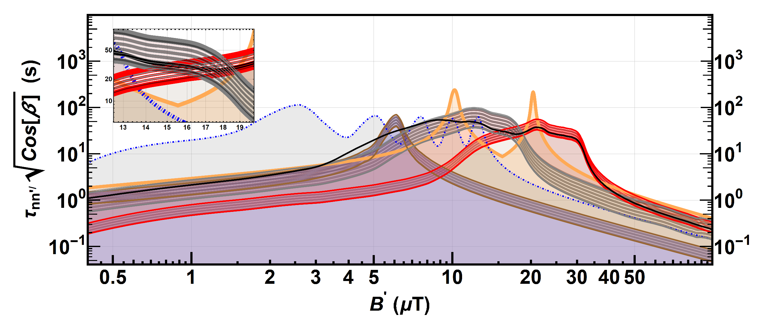
3.3. Projected Sensitivity Based on 2020 Measurements and Field Simulations

Based on the measured sensitivity of the asymmetry in counts for B-up and B-down field configurations we can estimate the 95% C.L. for the characteristic oscillation time. Since we have an inhomogeneous magnetic field in the chamber, we used in the simulation a field map obtained from previous coil calculations as illustrated in Figure 8. We included a background field and assumed perfect symmetry in the B-up and B-down fields. The calculation method of the sensitivity in $\tau$ for the inhomogeneous field case was as described in detail in refs. [62,84]. With 670 cycles per B field value, obtained in about 3.5 days, one can test the potential signals as shown in Figure 19, for example in a 1.0 μT interval at $B^{\prime }$ = 12.5 μT or a 1.5 μT interval at 25 μT.

4. Measurement Plans

The upgrade of the apparatus was carried out in spring 2021. The collaboration took data for 14 weeks of beamtime at the PSI West-1 UCN beamport in 2021.

During the main physics data-taking campaign, we focused on the regions compatible with potential signals reported by previous experiments, illustrated in Figure 1 by the red and gray bands. We used the storage technique illustrated in Section 2.1 to measure several cycles with the applied magnetic field inverted in a pattern to allow the compensation of all relevant drifts in the neutron counts. This technique was successfully demonstrated in the test measurement campaign.

The field ranges to be scanned, in order of priority, were:

• 12 μT–19 μT, compatible with potential signals reported by two previous experiments—[56,62]—where the red and grey bands in Figure 1 overlap;
• 22 μT–40 μT and 5 μT–10 μT, compatible with the potential signals found in [56] and [55] respectively;
• 40 μT–360 μT, where experimental bounds are very weak and could be substantially improved by a short data-taking run.

5. Summary

In this paper we present a new dedicated experiment to search for possible neutron to mirror-neutron oscillations in the presence of mirror magnetic fields. A first iteration was constructed and tested in fall 2020. Following an upgrade program and a detailed measurement of the magnetic field within the UCN storage chamber, a main data-taking run took place in 2021 at the West-1 beamline of the PSI UCN source. With a 14-week measurement period, we aim to either confirm a signal at a given mirror magnetic field or to fully exclude a large relevant and as of yet not constrained parameter space consistent with previously reported potential signals.

References

1. Lee, T.D.; Yang, C.-N. Question of Parity Conservation in Weak Interactions. Phys. Rev. 1956, 104, 254–258. [Google Scholar] [CrossRef]
2. Yu, I.; Kobzarev, L.; Okun, B.; Ya, I. Pomeranchuk, On the possibility of experimental observation of mirror particles. Sov. J. Nucl. Phys. 1966, 3, 837–841. [Google Scholar]
3. Foot, R.; Lew, H.; Volkas, R.R. A Model with fundamental improper space-time symmetries. Phys. Lett. B 1991, 272, 67–70. [Google Scholar] [CrossRef]
4. Berezhiani, Z. Mirror world and its cosmological consequences. Int. J. Mod. Phys. A 2004, 19, 3775–3806. [Google Scholar] [CrossRef]
5. Berezhiani, Z. Through the looking-glass: Alice’s adventures in mirror world. In From Fields to Strings: Circumnavigating Theoretical Physics; World Scientific Publishing Co Pte Ltd.: Singapore, 2005; Volume 3, pp. 2147–2195. [Google Scholar]
6. Foot, R. Mirror dark matter: Cosmology, galaxy structure and direct detection. Int. J. Mod. Phys. A 2014, 29, 1430013. [Google Scholar] [CrossRef] [Green Version]
7. Okun, L.B. Mirror particles and mirror matter: 50 years of speculations and search. Phys. Usp. 2007, 50, 380–389. [Google Scholar] [CrossRef] [Green Version]
8. Berezhiani, Z.; Comelli, D.; Villante, F.L. The Early mirror universe: Inflation, baryogenesis, nucleosynthesis and dark matter. Phys. Lett. B 2001, 503, 362–375. [Google Scholar] [CrossRef] [Green Version]
9. Ignatiev, A.Y.; Volkas, R.R. Mirror dark matter and large scale structure. Phys. Rev. D 2003, 68, 023518. [Google Scholar] [CrossRef] [Green Version]
10. Berezhiani, Z.; Ciarcelluti, P.; Comelli, D.; Villante, F.L. Structure formation with mirror dark matter: CMB and LSS. Int. J. Mod. Phys. D 2005, 14, 107–120. [Google Scholar] [CrossRef] [Green Version]
11. Berezhiani, Z.; Dolgov, A.; Mohapatra, R. Asymmetric inflationary reheating and the nature of mirror universe. Phys. Lett. B 1996, 375, 26–36. [Google Scholar] [CrossRef] [Green Version]
12. Berezhiani, Z.G. Astrophysical implications of the mirror world with broken mirror parity. arXiv 1996, arXiv:9602326. [Google Scholar]
13. Berezhiani, Z.; Cassisi, S.; Ciarcelluti, P.; Pietrinferni, A. Evolutionary and structural properties of mirror star MACHOs. Astropart. Phys. 2006, 24, 495–510. [Google Scholar] [CrossRef] [Green Version]
14. Holdom, B. Two U(1)’s and Epsilon Charge Shifts. Phys. Lett. B 1986, 166, 196–198. [Google Scholar] [CrossRef]
15. Glashow, S.L. Positronium Versus the Mirror Universe. Phys. Lett. B 1986, 167, 35–36. [Google Scholar] [CrossRef]
16. Berezhiani, Z.; Lepidi, A. Cosmological bounds on the ’millicharges’ of mirror particles. Phys. Lett. B 2009, 681, 276–281. [Google Scholar] [CrossRef] [Green Version]
17. Vigo, C.; Gerchow, L.; Radics, B.; Raaijmakers, M.; Rubbia, A.; Crivelli, P. New bounds from positronium decays on massless mirror dark photons. Phys. Rev. Lett. 2020, 124, 101803. [Google Scholar] [CrossRef] [Green Version]
18. Berezhiani, Z.; Dolgov, A.D.; Tkachev, I.I. Dark matter and generation of galactic magnetic fields. Eur. Phys. J. C 2013, 73, 2620. [Google Scholar] [CrossRef] [Green Version]
19. Foot, R. Mirror dark matter and the new DAMA/LIBRA results: A Simple explanation for a beautiful experiment. Phys. Rev. D 2008, 78, 043529. [Google Scholar] [CrossRef] [Green Version]
20. Cerulli, R.; Villar, P.; Cappella, F.; Bernabei, R.; Belli, P.; Incicchitti, A.; Addazi, A.; Berezhiani, Z. DAMA annual modulation and mirror Dark Matter. Eur. Phys. J. C 2017, 77, 83. [Google Scholar] [CrossRef] [Green Version]
21. Addazi, A.; Berezhiani, Z.; Bernabei, R.; Belli, P.; Cappella, F.; Cerulli, R.; Incicchitti, A. DAMA annual modulation effect and asymmetric mirror matter. Eur. Phys. J. C 2015, 75, 400. [Google Scholar] [CrossRef] [Green Version]
22. Berezhiani, Z. Unified picture of the particle and sparticle masses in SUSY GUT. Phys. Lett. B 1998, 417, 287–296. [Google Scholar] [CrossRef] [Green Version]
23. Belfatto, B.; Berezhiani, Z. How light the lepton flavor changing gauge bosons can be. Eur. Phys. J. C 2019, 79, 202. [Google Scholar] [CrossRef]
24. Belfatto, B.; Beradze, R.; Berezhiani, Z. The CKM unitarity problem: A trace of new physics at the TeV scale? Eur. Phys. J. C 2020, 80, 149. [Google Scholar] [CrossRef]
25. Addazi, A.; Berezhiani, Z.; Kamyshkov, Y. Gauged B-L number and neutron–antineutron oscillation: Long-range forces mediated by baryophotons. Eur. Phys. J. C 2017, 77, 301. [Google Scholar] [CrossRef] [Green Version]
26. Babu, K.S.; Mohapatra, R.N. Limiting Equivalence Principle Violation and Long-Range Baryonic Force from Neutron-Antineutron Oscillation. Phys. Rev. D 2016, 94, 054034. [Google Scholar] [CrossRef] [Green Version]
27. Rubakov, V.A. Grand unification and heavy axion. JETP Lett. 1997, 65, 621–624. [Google Scholar] [CrossRef]
28. Berezhiani, Z.; Gianfagna, L.; Giannotti, M. Strong CP problem and mirror world: The Weinberg-Wilczek axion revisited. Phys. Lett. B 2001, 500, 286–296. [Google Scholar] [CrossRef] [Green Version]
29. Sakharov, A.D. Violation of CP Invariance, C asymmetry, and baryon asymmetry of the universe. JETP Lett. 1967, 5, 24. [Google Scholar] [CrossRef] [Green Version]
30. Bento, L.; Berezhiani, Z. Leptogenesis via Collisions: Leaking Lepton Number to the Hidden Sector. Phys. Rev. Lett. 2001, 87, 231304. [Google Scholar] [CrossRef] [Green Version]
31. Bento, L.; Berezhiani, Z. Baryon asymmetry, dark matter and the hidden sector. Fortsch. Phys. 2002, 50, 489–495. [Google Scholar] [CrossRef]
32. Berezhiani, Z. Unified picture of ordinary and dark matter genesis. Eur. Phys. J. Spec. Top. 2008, 163, 271–289. [Google Scholar] [CrossRef]
33. Berezhiani, Z. Matter, dark matter, and antimatter in our Universe. Int. J. Mod. Phys. A 2018, 33, 1844034. [Google Scholar] [CrossRef]
34. Akhmedov, E.K.; Berezhiani, Z.G.; Senjanovic, G. Planck scale physics and neutrino masses. Phys. Rev. Lett. 1992, 69, 3013–3016. [Google Scholar] [CrossRef] [Green Version]
35. Foot, R.; Volkas, R. Neutrino physics and the mirror world: How exact parity symmetry explains the solar neutrino deficit, the atmospheric neutrino anomaly and the LSND experiment. Phys. Rev. D 1995, 52, 6595–6606. [Google Scholar] [CrossRef] [Green Version]
36. Berezhiani, Z.G.; Mohapatra, R.N. Reconciling present neutrino puzzles: Sterile neutrinos as mirror neutrinos. Phys. Rev. D 1995, 52, 6607–6611. [Google Scholar] [CrossRef] [Green Version]
37. Berezhiani, Z.; Bento, L. Neutron-mirror-neutron oscillations: How fast might they be? Phys. Rev. Lett. 2006, 96, 081801. [Google Scholar] [CrossRef] [Green Version]
38. Phillips, D.G., II. Neutron-Antineutron Oscillations: Theoretical Status and Experimental Prospects. Phys. Rep. 2016, 612, 1–45. [Google Scholar] [CrossRef] [Green Version]
39. Baldo-Ceolin, M.; Benetti, P.; Bitter, T.; Bobisut, F.; Calligarich, E.; Dolfini, R.; Dubbers, D.; El-Muzeini, P.; Genoni, M.; Gibin, D.; et al. A new experimental limit on neutron-antineutron oscillations. Zeit. F. Phys. C 1994, 63, 409–416. [Google Scholar] [CrossRef] [Green Version]
40. Abe, K. Search for n-nbar oscillation in Super-Kamiokande. arXiv 2011, arXiv:1109.4227v2.2011. [Google Scholar]
41. Berezhiani, Z. More about neutron—Mirror neutron oscillation. Eur. Phys. J. C 2009, 64, 421–431. [Google Scholar] [CrossRef] [Green Version]
42. Berezhiani, Z.; Bento, L. Fast neutron-mirror-neutron oscillation and ultra high energy cosmic rays. Phys. Lett. B 2006, 635, 253–259. [Google Scholar] [CrossRef] [Green Version]
43. Berezhiani, Z.; Gazizov, A. Neutron Oscillations to Parallel World: Earlier End to the Cosmic Ray Spectrum? Eur. Phys. J. C 2012, 72, 2111. [Google Scholar] [CrossRef] [Green Version]
44. Mohapatra, R.N.; Nasri, S.; Nussinov, S. Some implications of neutron mirror neutron oscillation. Phys. Lett. B 2005, 627, 124–130. [Google Scholar] [CrossRef] [Green Version]
45. Berezhiani, Z.; Biondi, R.; Mannarelli, M.; Tonelli, F. Neutron-mirror neutron mixing and neutron stars. Eur. Phys. J. C 2021, 81, 1036. [Google Scholar] [CrossRef]
46. Goldman, I.; Mohapatra, R.N.; Nussinov, S. Bounds on neutron-mirror neutron mixing from pulsar timing. Phys. Rev. D 2019, 100, 123021. [Google Scholar] [CrossRef] [Green Version]
47. Ciancarella, R.; Pannarale, F.; Addazi, A.; Marciano, A. Constraining mirror dark matter inside neutron stars. Phys. Dark Univ. 2021, 32, 100796. [Google Scholar] [CrossRef]
48. Coc, A.; Pospelov, M.; Uzan, J.-P.; Vangioni, E. Modified big bang nucleosynthesis with nonstandard neutron sources. Phys. Rev. D 2014, 90, 085018. [Google Scholar] [CrossRef] [Green Version]
49. Berezhiani, Z. Neutron lifetime puzzle and neutron–mirror neutron oscillation. Eur. Phys. J. C 2019, 79, 484. [Google Scholar] [CrossRef] [Green Version]
50. Green, G.L.; Geltenbort, P. The neutron enigma. Sci. Am. 2016, 4, 29. [Google Scholar] [CrossRef]
51. Berezhiani, Z. Neutron-antineutron oscillation and baryonic majoron: Low scale spontaneous baryon violation. Eur. Phys. J. C 2016, 76, 705. [Google Scholar] [CrossRef] [Green Version]
52. Berezhiani, Z. A possible shortcut for neutron–antineutron oscillation through mirror world. Eur. Phys. J. C 2021, 81, 33. [Google Scholar] [CrossRef]
53. Pokotilovski, N. On the experimental search for neutron → mirror neutron oscillations. Phys. Lett. B 2006, 639, 214–217. [Google Scholar] [CrossRef] [Green Version]
54. Berezhiani, Z.; Frost, M.; Kamyshkov, Y.; Rybolt, B.; Varriano, L. Neutron disappearance and regeneration from a mirror state. Phys. Rev. D 2017, 96, 035039. [Google Scholar] [CrossRef] [Green Version]
55. Ban, G.; Bodek, K.; Daum, M.; Henneck, R.; Heule, S.; Kasprzak, M.; Khomutov, N.; Kirch, K.; Kistryn, S.; Knecht, A.; et al. Direct experimental limit on neutron—Mirror-neutron oscillations. Phys. Rev. Lett. 2007, 99, 161603. [Google Scholar] [CrossRef] [Green Version]
56. Serebrov, A.; Aleksandrov, E.; Dovator, N.; Dmitriev, S.; Fomin, A.; Geltenbort, P.; Kharitonov, A.; Krasnoschekova, I.; Lasakov, M.; Murashkin, A.; et al. Experimental search for neutron-mirror neutron oscillations using storage of ultracold neutrons. Phys. Lett. B 2008, 663, 181–185. [Google Scholar] [CrossRef] [Green Version]
57. Abel, C.; Ayres, N.J.; Ban, G.; Bison, G.; Bodek, K.; Bondar, V.; Chanel, E.; Chiu, P.-J.; Crawford, C.; Daum, M.; et al. A search for neutron to mirror-neutron oscillations using the nEDM apparatus at PSI. Phys. Lett. B 2021, 812, 135993. [Google Scholar] [CrossRef]
58. Altarev, I.; Baker, C.A.; Ban, G.; Bodek, K.; Daum, M.; Fierlinger, P.; Geltenbort, P.; Green, K.; Grinten, M.G.D.V.; Gutsmiedl, E.; et al. Neutron to Mirror-Neutron Oscillations in the Presence of Mirror Magnetic Fields. Phys. Rev. D 2009, 80, 032003. [Google Scholar] [CrossRef] [Green Version]
59. Serebrov, A.P.; Aleksandrov, E.B.; Dovator, N.A.; Dmitriev, S.P.; Fomin, A.K.; Geltenbort, P.; Kharitonov, A.G.; Krasnoschekova, I.A.; Lasakov, M.S.; Murashkin, A.N.; et al. Search for neutron-mirror neutron oscillations in a laboratory experiment with ultracold neutrons. Nucl. Instrum. Meth. A 2009, 611, 137–140. [Google Scholar] [CrossRef] [Green Version]
60. Bodek, K.; Kistryn, S.; Kuźniak, M.; Zejma, J.; Burghoff, M.; Knappe-Grüneberg, S.; Sander-Thoemmes, T.; Schnabel, A.; Trahms, L.; Ban, G.; et al. Additional results from the first dedicated search for neutronmirror neutron oscillations. Nucl. Instrum. Meth. A 2009, 611, 141–143. [Google Scholar] [CrossRef]
61. Berezhiani, Z.; Nesti, F. Magnetic anomaly in UCN trapping: Signal for neutron oscillations to parallel world? Eur. Phys. J. C 2012, 72, 1974. [Google Scholar] [CrossRef] [Green Version]
62. Berezhiani, Z.; Biondi, R.; Geltenbort, P.; Krasnoshchekova, I.; Varlamov, V.; Vassiljev, A.; Zherebtsov, O. New experimental limits on neutron-mirror neutron oscillations in the presence of mirror magnetic field. Eur. Phys. J. C 2018, 78, 717. [Google Scholar] [CrossRef] [Green Version]
63. MohanMurthy, P.T. A Search for Neutron to Mirror-Neutron Oscillations. Ph.D. Thesis, ETH Zurich, Zürich, Switzerland, 2019. No. 26525. [Google Scholar]
64. Broussard, L.J.; Barrow, J.L.; DeBeer-Schmitt, L.; Dennis, T.; Fitzsimmons, M.R.; Frost, M.J.; Gilbert, C.E.; Gonzalez, F.M.; Heilbronn, L.; Iverson, E.B.; et al. Experimental Search for Neutron to Mirror Neutron Oscillations as an Explanation of the Neutron Lifetime Anomaly. arXiv 2021, arXiv:2111.05543. [Google Scholar]
65. Bison, G.; Blau, B.; Daum, M.; Goeltl, L.; Henneck, R.; Kirch, K.; Lauss, B.; Ries, D.; Schmidt-Wellenburg, P.; Zsigmond, G. Neutron optics of the PSI ultracold neutron source: Characterization and simulation. Eur. Phys. J. A 2020, 56, 33. [Google Scholar] [CrossRef]
66. Lauss, B. A New Facility for Fundamental Particle Physics: The High-Intensity Ultracold Neutron Source at the Paul Scherrer Institute. AIP Conf. Proc. 2012, 1441, 576–578. [Google Scholar] [CrossRef] [Green Version]
67. Lauss, B. Startup of the high-intensity ultracold neutron source at the Paul Scherrer Institute. Hyperf. Int. 2012, 211, 21–25. [Google Scholar] [CrossRef] [Green Version]
68. Lauss, B. Ultracold Neutron Production at the Second Spallation Target of the Paul Scherrer Institute. Phys. Proc. 2014, 51, 98. [Google Scholar] [CrossRef] [Green Version]
69. Bison, G.; Daum, M.; Kirch, K.; Lauss, B.; Ries, D.; Schmidt-Wellenburg, P.; Zsigmond, G.; Brenner, T.; Geltenbort, P.; Jenke, T.; et al. Comparison of ultracold neutron sources for fundamental physics measurements. Phys. Rev. C 2017, 95, 045503. [Google Scholar] [CrossRef] [Green Version]
70. Lauss, B.; Blau, B. UCN, the ultracold neutron source—Neutrons for particle physics. SciPost Phys. Proc. 2021, 5, 004. [Google Scholar] [CrossRef]
71. Daum, M.; Franke, B.; Geltenbort, P.; Gutsmiedl, E.; Ivanov, S.; Karch, J.; Kasprzak, M.; Kirch, K.; Kraft, A.; Lauer, T.; et al. Transmission of ultra-cold neutrons through guides coated with materials of high optical potential. Nucl. Instrum. Methods A 2014, 741, 71–77. [Google Scholar] [CrossRef]
72. Blau, B.; Daum, M.; Fertl, M.; Geltenbort, P.; Goeltl, L.; Henneck, R.; Kirch, K.; Knecht, A.; Lauss, B.; Schmidt-Wellenburg, P.; et al. A prestorage method to measure neutron transmission of ultracold neutron guides. Nucl. Instrum. Methods A 2016, 807, 30–40. [Google Scholar] [CrossRef] [Green Version]
73. Bison, G.; Burri, F.; Daum, M.; Kirch, K.; Krempel, J.; Lauss, B.; Meier, M.; Ries, D.; Schmidt-Wellenburg, P.; Zsigmond, G. An ultracold neutron storage bottle for UCN density measurements. Nucl. Instrum. Methods A 2016, 830, 449. [Google Scholar] [CrossRef] [Green Version]
74. Brys, T.; Czekaj, S.; Daum, M.; Fierlinger, P.; George, D.; Henneck, R.; Kasprzak, M.; Kirch, K.; Kuzniak, M.; Kuehne, G.; et al. Magnetic field stabilization for magnetically shielded volumes by external field coils. Nucl. Inst. Meth. A 2005, 554, 527–539. [Google Scholar] [CrossRef] [Green Version]
75. Afach, S.; Bison, G.; Bodek, K.; Burri, F.; Chowdhuri, Z.; Daum, M.; Fertl, M.; Franke, B.; Grujić, Z.D.; Hélaine, V.; et al. Dynamic stabilization of the magnetic field surrounding the neutron electric dipole moment spectrometer at the Paul Scherrer Institute. J. Appl. Phys. 2014, 116, 084510. [Google Scholar] [CrossRef] [Green Version]
76. Abel, C.; Ayres, N.J.; Ban, G.; Bison, G.; Bodek, K.; Bondar, V.; Chanel, E.; Chiu, P.-J.; Clément, B.; Crawford, C.B.; et al. Mapping of the magnetic field to correct systematic effects in a neutron electric dipole moment experiment. arXiv 2021, arXiv:2103.09039. [Google Scholar]
77. Ayres, N.J.; Ban, G.; Bienstman, L.; Bison, G.; Bodek, K.; Bondar, V.; Bouillaud, T.; Chanel, E.; Chen, J.; Chiu, P.-J.; et al. The design of the n2EDM experiment. Eur. Phys. J. C 2021, 81, 512. [Google Scholar] [CrossRef]
78. Rozpedzik, D.; Bodek, K.; Lauss, B.; Ries, D.; Schmidt-Wellenburg, P.; Zsigmond, G. Oscillating ultra-cold neutron spectrometer. EPJ Web Conf. 2019, 219, 10007. [Google Scholar] [CrossRef] [Green Version]
79. Anghel, A.; Bailey, T.L.; Bison, G.; Blau, B.; Broussard, L.J.; Clayton, S.M.; Cude-Woods, C.; Daum, M.; Hawari, A.; Hild, N.; et al. Solid deuterium surface degradation at ultracold neutron sources. Eur. Phys. J. A 2018, 54, 148. [Google Scholar] [CrossRef]
80. Zsigmond, G. The MCUCN simulation code for ultracold neutron physics. Nucl. Instrum. Methods A 2018, 881, 16–26. [Google Scholar] [CrossRef] [Green Version]
81. Ries, D. Characterisation and Optimisation of the Source for Ultracold Neutrons at the Paul Scherrer Institute. Ph.D. Thesis, ETH, Zürich, Switzerland, 2016. No. 23671. [Google Scholar]
82. Bison, G.; Daum, M.; Kirch, K.; Lauss, B.; Ries, D.; Schmidt-Wellenburg, P.; Zsigmond, G. Ultracold neutron storage and transport at the PSI UCN source. arXiv 2021, arXiv:2110.12988. [Google Scholar]
83. Golub, R.; Richardson, D.J.; Lamoreaux, S.K. Ultra-Cold Neutrons; CRC Press: Boca Raton, FL, USA, 1991. [Google Scholar]
84. Biondi, R. Monte Carlo simulation for ultracold neutron experiments searching for neutron–mirror neutron oscillation. Int. J. Mod. Phys. A 2018, 33, 1850143. [Google Scholar] [CrossRef] [Green Version]
Figure 1. Limit on n n oscillation times normalized by the square root of the cosine of the angle β between the magnetic field B in vertical direction and the unknown field B . The figure is from the recent publication of the nEDM collaboration [57]. White regions are still allowed. The solid orange curve represents the lower limit from [57]. The solid black curve is the global constraint calculated in [62] considering data from [55,58,59,62]. The dashed blue curve is from [58]. The red region bounded by red lines peaking above 20 μT is the 95% C.L. signal region recalculated in [62] from the 5.2 σ deviation observed in [61] in the experimental data of [56]. The brown region bounded by brown lines peaking at around 6 μT is the 95% C.L. signal region calculated by the same Ref. [62] from a 3 σ deviation in [55]. The gray region bounded by dashed gray lines indicates the 95% C.L. region for the 2.5 σ deviation observed in the B2 series of experiment [62]. The angle of 2.9° between the vertical axes at the geographic locations of PSI and ILL introduces a small additional source of uncertainty when comparing exclusion plots from measurements at PSI and ILL, respectively. Reproduced with permission under the Creative Commons CC-BY license. Indicated changes are: the upper part of the figure was omitted in this reproduction and the citations given in the figure removed.
Symmetry 14 00503 g001
Figure 2. Illustration of steps of a “storage” type measurement. Indicated in the figure are turbo-molecular pumps (TP1, TP2, TP3), shutters (SH1, SH2, SH3, B_SH), vacuum gauges (VG1, VG2, VG3), and valve (V1). (Not to scale). The operation sequence is the following: Ready—setup is waiting for the beam pulse and pumping; Filling—UCNs enter the storage vessel with SH2 and SH3 closed; Monitoring—after filling a short monitoring period, with SH2 open, is used to determine the UCN intensity; Storage—SH1 and SH2 is closed and UCNs are stored for a set time if 120 s in the storage vessel; Counting—SH2 is opened and UCNs are counted in the detector.
Symmetry 14 00503 g002
Figure 3. Time spectrum of UCN counts in the UCN detector for a single “storage” type measurement.
Symmetry 14 00503 g003
Figure 4. Illustration of steps of a “leakage” type measurement. Shutter SH3 was lowered to the bottom of the storage vessel allowing thus to define a specific leakage rate, and the top opening (for pumping) was closed with an additional plate. The operating procedure is: Ready—the setup is waiting for the beam pulse and pumping; Filling—UCNs are filled into the storage vessel and the emptying guide up to the detector (SH2 open); Counting—shutter SH1 is closed and all UCN are stored in the storage vessel and counted simultaneously in the detector (SH2 open).
Symmetry 14 00503 g004
Figure 5. Time spectrum of UCN counts in the UCN detector for a single “leakage” type measurement. Monitoring and counting periods are indicated with dashed lines.
Symmetry 14 00503 g005
Figure 6. Cut view of the experiment as installed in area West-1 in fall 2020: (1) beamport shutter; (2) UCN guides (275 cm); (3) storage vessel (filling) shutter SH1; (4) vacuum vessel containing the storage chamber; (5) storage vessel (emptying) shutter SH2; (6) UCN detector; (7) coil system for B-field generation in directions x—blue, y—red, z—green; (8) top hole opened during pumping (can be closed by shutter SH3 in storage measurements); (9) concrete shielding.
Symmetry 14 00503 g006
Figure 7. Photo of the experiment setup in the UCN area West during the test measurements in fall 2020. The visible parts can be compared with the description given in Figure 6. The UCN glass guides (on the right hand side) leading from beamport West-1 to the apparatus are covered by folded sheet metal pieces for protection. The visible metal frame supports the coil-windings, the wooden frame supports the fluxgates.
Symmetry 14 00503 g007
Figure 8. Simulated magnetic field map based on a coil configuration before full optimization. The simulation is based on an analytical calculation using the Biot–Savart law, with coil currents set to produce a nominal field of 100 μT. The left plot shows a histogram of B z B z m e a n at a large number of points distributed randomly throughout the cylindrical storage volume (note the logarithmic y-axis). The right plot shows a slice of the computed field deviation in the x y plane cut at z = 0 i.e., the center of the storage volume, with x and y in meters. This calculation assumes linearity, so the deviations in microtesla from a uniform 100 μT field are equivalent to a percentage deviation from an arbitrary field. The real apparatus used an optimized coil geometry, however here we present calculations using a “realistically bad” configuration to estimate the impact of uncompensated inhomogeneities.
Symmetry 14 00503 g008
Figure 9. Photo of the prototype magnetic-field mapper mounted in a test stand in the lab at ETH Zurich. The central axle can slide freely through flanges to be mounted on the top and bottom of the vacuum tank, allowing the height and rotation of the arm to be manipulated from outside with the tank closed. Several fluxgates can be mounted at different radii on the arm, allowing almost the full 3D volume to be mapped. All parts are non-magnetic.
Symmetry 14 00503 g009
Figure 10. Measured storage curve using the “storage” technique. The data-points represent the mean of the normalized UCN counts measured in 10 measurement cycles (i.e., as explained in Figure 2) per point. Error bars are smaller than the symbols. The found ‘long’ storage time constant of 85 s was sufficient to propose the experiment at PSI, however, it was improved considerably due to the electropolishing for the 2021 data-taking campaign (see Section 2.3).
Symmetry 14 00503 g010
Figure 11. Example measurement demonstrating the time variation of the UCN counts over around 1.5 days of normal running, all normalized to 1 at the start. The length of one measurement cycle is given by the 5 min between two proton beam pulses onto the UCN source. Blue squares—integrated counts C S observed after storage; red circles—integrated counts C M observed during the monitoring interval; black stars—normalized counts C S / C M .
Symmetry 14 00503 g011
Figure 12. Representative time series of the count asymmetry computed for 54 sequences with opposite magnetic fields A and B, as defined in the text (12.5 μT for this example). As shown on the right, the mean of the asymmetry values is compatible with zero and the scatter is compatible to what would be expected for pure Poisson statistics. This demonstrates the suitability of our method to compensate for small variations in the UCN source output.
Symmetry 14 00503 g012
Figure 13. MCUCN model of the n n experiment at the PSI UCN source. The blue dots are calculated reflection points of the UCN illuminating the guides and the storage volume. The open shutter towards the detector is visible. The two larger cylindrical volumes on the side and the bottom represent the “pocket” volumes as explained in the text.
Symmetry 14 00503 g013
Figure 14. Measured and simulated UCN storage curve with benchmarked parameters. The simulation was normalized to the experimental curve for better comparison.
Symmetry 14 00503 g014
Figure 15. Measured and simulated UCN emptying curves validating that the parameters benchmarked from the storage curves are correct.
Symmetry 14 00503 g015
Figure 16. Distribution of the free-flight-time t f histogrammed between 115 and 120 s of storage. The thin curve represents the distribution for UCN that only bounce at the wall of the large chamber, i.e., without considering reflections in the attached guide sections (“pockets”). The values indicated in the legend are: mean—mean value of t f ; SD—standard deviation; and SE—standard error of mean.
Symmetry 14 00503 g016
Figure 17. Simulated reflection points in a MCUCN setup with 0.5 m elevated UCN storage chamber using uncoated stainless steel guides.
Symmetry 14 00503 g017
Figure 18. Gain factors for various improvement scenarios, with respect to storage time, see text for details.
Symmetry 14 00503 g018
Figure 19. Simulated exclusion curves at 95% C.L. corresponding to 670 cycles, equivalent to 3.5 days of data taking, per field value for two examples of the central field, 12.5 μT and 25 μT. The claimed potential signals were also plotted as reference represented by the bands bordered by the lines of same color.
Symmetry 14 00503 g019