
Low-Energy Interactions of Mesons with Participation of the First Radially Excited States in U(3) × U(3) NJL Model


1
Bogoliubov Laboratory of Theoretical Physics, Joint Institute for Nuclear Research, 141980 Dubna, Russia
2
Institute of Nuclear Physics, Almaty 050032, Kazakhstan
3
Faculty of Physics and Technology, Al-Farabi Kazakh National University, Almaty 050040, Kazakhstan
*
Author to whom correspondence should be addressed.
Symmetry 2022, 14(2), 308; https://doi.org/10.3390/sym14020308
Submission received: 30 December 2021
/
Revised: 17 January 2022
/
Accepted: 1 February 2022
/
Published: 2 February 2022
(This article belongs to the Special Issue Symmetry in Quantum Field Theory, Critical Behavior Theory and Stochastic Dynamics)
Abstract
:The chiral symmetric NJL model describing pseudoscalar, vector, and axial-vector mesons in both the ground state and first radially excited states is shortly presented in this review. In this model, it is possible to describe a large number of low-energy interactions of mesons, lepton decays into mesons, and processes of meson production in electron–positron annihilations in satisfactory agreement with the experiments. In describing a number of processes, it turned out to be necessary to take into account the interactions of mesons in the final state.
1. Introduction
Studies of meson interactions at low energies are of great interest for investigations of both the nature of the intrinsic properties and their interaction with each other. Such studies are carried out from both the theoretical and experimental points of view. Among the experimental centers, we can note world scientific centers such as VEPP-2000 (Budker INP, Novosibirsk), UNK (IHEP, Protvino), BaBar (SLAC, USA), Belle (KEK, Japan), BES III (BEPC II, China), LEP (CERN), etc.
For a theoretical description of processes in the interested energy region below ∼2 GeV, use of the well-developed QCD perturbation theory is unfortunately impossible due to a large value of the coupling constant. Therefore, as a rule, various phenomenological theories are applied here. These theories are based on the use of characteristic symmetries to which the corresponding interactions of elementary particles conform. One of the main symmetries of this kind is chiral symmetry. These symmetries were widely used even before the construction of the fundamental QCD theory [1,2,3,4,5,6,7,8].
Among various models closely related to internal symmetries of strong interactions, the Nambu–Jona-Lasinio model, proposed in 1961 [9], can be considered very successful. In the quark language, this model was first formulated in [10,11]. Later, it was actively developed by many authors since the 1980s, e.g., in [12,13,14,15,16,17,18,19,20,21,22,23,24]. All these works are quite similar and differ mainly in different definitions of the internal parameters. In this review, we will use the version of the NJL model, described in [13,16,20,22,24].
In the low-energy region, an important role in addition to the ground states of mesons is also played by the first radial excitations. This especially concerns the processes of meson production in colliding beams as well as lepton decays. An important role in the description of these processes is played by channels containing mesons in both the ground and first radially excited states. Therefore, for a satisfactory description of these processes, the symmetric extended NJL model was formulated in 1997 [25,26]. This model was used to describe many processes involving radially excited mesons. However, this model turned out to be especially useful for describing lepton decays. Note that taking into account intermediate mesons with higher powers of excitation in decays can only lead to insignificant corrections within the accuracy of the model. The masses of these mesons turn out to be much heavier and, as a rule, exceed the value of the lepton mass.
The structure of the review is organized as follows. In Section 2, we will present the chiral NJL model that describes only the ground meson states. The Lagrangians of the quark–meson interactions will be obtained and the values of the constituent and current masses of the u, d, and s quarks will be found. Taking into account the t’Hooft interaction, the mixing angle of the and mesons will be defined. When describing kaons, the possibility of mixing and mesons will be taken into account.
In Section 3, the extended NJL model will be described, the mixing angles of the ground and first radially excited states of mesons will be found, and the interaction Lagrangians of radially excited mesons with quarks will be constructed. In Section 4, a table containing the decay widths of radially excited mesons, calculated by proposed the extended NJL model will be given. In this section, a number of meson production processes in beams will be considered.
2. The Standard Nambu–Jona-Lasinio Model
2.1. The NJL Model
2.1.1. Lagrangian for Scalar, Pseudoscalar, Vector, and Axial-Vector Mesons
In this section, we will show the construction of the standard NJL model following the works [13,16,20,24]. The quark Lagrangian containing the four-quark interaction motivated by the fundamental QCD theory in the local approximation has the form
where are the u and d quark fields, is the current quark mass matrix, , are the four-quark coupling constants, and are the Pauli matrices.
The meson fields are introduced using functional integrations [27]. After the introduction of meson fields, the Lagrangian (1) takes the form
It is easy to verify that in this expression the vacuum expectation of the scalar field is not equal to zero, which requires a redefinition of the vacuum. This redefinition of the scalar field is achieved by subtracting from it the nonzero vacuum expectation of the scalar field and adding this value to the current quark mass: . The described actions lead to the spontaneous breaking of chiral symmetry. The values of the current and constituent quark masses are determined by the gap equation
In the one-loop quark approximation (Figure 1), we obtain the following free Lagrangian for scalar and pseudoscalar meson fields:
Similarly, for the free Lagrangian of vector and axial-vector mesons, we obtain
Here, the field renormalization constants are expressed in terms of the logarithmic divergent integral
From the obtained formulas, the connection between the constants and follows
The mass formulas for the mesons and have the form
The constants of the four-quark interactions and will be determined from these formulas using the experimental values of the and mesons masses in Section 2.1.2.
Expressions for quadratically and logarithmically diverging integrals arising when considering quark loops have the form
where is the number of colors in QCD and is the cutoff parameter. The numerical values of the model parameters included in these integrals will be indicated below.
Due to the existence of transitions between pseudoscalar and axial-vector mesons, non-diagonal terms appear in the Lagrangian. This leads to additional renormalization of the pion field, which is absent in scalar fields. This renormalization has the form
As a result, for the interaction Lagrangian of quarks with , , and mesons, we obtain
where .
2.1.2. Numerical Estimates of the Model Parameters
Let us now determine the main parameters of the model: the masses of the constituent light quarks , the ultraviolet cut-off parameter , and the constants , . To determine the masses of the constituent quarks and the ultraviolet cut-off parameter of the quark loops, two equations will be used from the experimental values of the decay widths ( MeV) and the strong decay () [28].
When calculating quark loops in our model, we will use the lowest order in the expansion of , and also take into account only terms with minimum powers in external momenta. Under this condition, is it possible to maintain the chiral-symmetric structure of the meson interaction Lagrangian at low energies [16].
The decay in the NJL model with transitions is described by the following amplitudes:
where is the Fermi constant, is the element of the Cabibbo–Kobayashi–Maskawa matrix and is the lepton current.
In this case, we obtain the Goldberger–Treiman relation for the weak decay constant
Using the relationship between the constants (7) and (10), we obtain the following equation for the constituent quark mass:
The cut-off parameter MeV is found using the constant , which is expressed through the integral (6). Note that while using the value , this cut-off parameter has turned out to be noticeable more than in other versions of the NJL model [18,19]. As it will be shown below this allow to include the first radially excited meson states within the chiral symmetric extended NJL model (see Section 3).
The values of the constants and are determined from the equations for the masses of the pion and vector mesons (8)
The value of the current quark mass is found from the gap Equation (3), which gives MeV.
We now turn to the description of the decay, which will allow us to estimate the difference between the u and d quark masses. The amplitude of this decay contains contributions from the strong and electromagnetic transitions [16]
where
Here, , , , and are vector meson masses and , are the momenta of and mesons.
2.2. The NJL Model
When extending the model for the group , the Pauli matrices are replaced by the Gell–Mann matrices , where is the matrix proportional to the identity one. Instead of quark doublets we have quark triplets , and the current mass matrix is replaced by the matrix
Pseudoscalar, vector, and axial-vector mesons are introduced into the model in the same way as it was done in the one.
As a result, after bosonization of the quark Lagrangian, we obtain the following mass formulas for mesons containing s quarks:
The mass formulas for non-strange mesons remain unchanged.
The renormalization constants of the vector fields and are defined in terms of the integrals
where
When deriving the free Lagrangian for the kaon, we take into account additional renormalization of the kaon field () due to possible transitions between the pseudoscalar and axial-vector mesons. Here, it is necessary to take into account two physical axial-vector states and . They are the result of mixing of two axial-vector strange mesons , and related to each other by the following relations:
In the case of the chiral group , the axial-vector mesons from the nonet and from the nonet do not mix with each other. This is a consequence of the fulfillment of chiral symmetry and the proximity of the constituent u and d quark masses. Therefore, when describing the transitions, the pion has only one partner among the axial-vector mesons, namely, .
At the same time, for the group, due to a large mass difference between and , chiral symmetry is noticeably broken, and the states and begin to mix with a coupling constant proportional to the mass difference . As a consequence, physically observed axial-vector mesons begin to have masses MeV and MeV [29]. The NJL model describes only the meson . Further, we will denote it just . As a result, for the renormalization constant, we obtain
where
where [30].
2.3. The ’t Hooft Interaction
After the introduction of a heavier s quark into our model, in the framework of the group, ideal mixing occurs between the eighth representative of the pseudoscalar meson octet and the pseudoscalar singlet meson. Moreover, one of these states contains only u and d quarks, while the other contains only s quarks, which contradicts the experimental data. To solve this problem, it is also necessary to take into account the ’t Hooft interaction, which leads to mixing of the states containing light quarks with the heavier s quark [31,32]. Taking into account the ’t Hooft interaction allows us to correctly describe the masses of the pseudoscalar mesons and . This interaction has the form [33]
where are the antiquark fields, is the diagonal matrix of current quark masses , , and K is the ’t Hooft constant.
To describe the NJL model, we can combine the six-quark interaction with the initial four-quark interaction. In this case, we use the method of separating the main four-quark interaction from the ’t Hooft six-quark interaction. The details of these procedures are fairly well described in many papers, in particular in [18,19,24,31]. Therefore, omitting the details, we write the new Lagrangian in the following form (see the papers in [24,31]):
where
For the and mesons masses, taking into account the mixing of , and s quarks caused by the ’t Hooft interaction, we obtain the following formulas:
where
where is the ideal mixing angle and is the singlet-octet mixing angle
The best agreement with the experimental values for the and mesons masses can be obtained for the value of the angle
For the ’t Hooft constant, we get the value . Here, we will not discuss scalar mesons, as the contribution of scalar mesons to the decays we are considering turns out to be negligible. In addition, a detailed description of the scalar sector in the NJL model can be found in our previous works [34,35]. Moreover, finally, at the moment there are many works describing scalar mesons taking into account their tetraquark state [36,37,38], while in the NJL model considered here, tetraquarks are not taken into account.
As a result, in the framework of the NJL model, we obtain the following interaction Lagrangian of quarks with strange mesons:
where
where matrices and are defined in (31).
The parameters used in this model, as noted in the introduction, differ markedly from the parameters used in other versions of the NJL model [19]. This difference causes our cut-off parameter to significantly exceed the cut-off parameter used in [19]. This circumstance allows us, within the framework of the chiral symmetric model, to describe not only the four main mesonic nonets, but also their first radial excitations. Taking into account intermediate mesons in the ground and first radially excited states in lepton decay turn out to be essential, while higher excitations play a less important role and can be neglected within the framework of the model’s accuracy. In the next section, we will show how, using the simplest form factor of the lowest order in momenta, one can describe the first radial excitations of mesons without going beyond the limits of the admissible breaking of chiral symmetry allowed by the requirement of the partial conservation of the axial current (PCAC) theorem.
The precision of the NJL model is determined on the basis of the PCAC. In the case of symmetry, it can be determined with the ratio [39]. There are a large number of other sources of uncertainties. Therefore, we use our previous results to estimate the error of the model. Without any exotic states, the average uncertainty can be estimated at the level of 10%. This error obtained from the real calculation covers all possible sources including PCAC and can be absorbed by it. Therefore, we estimate the uncertainty of this model at the level of 17%.
3. The Extended NJL Model
The extended NJL model was formulated in the works [25,26]. As it has been mentioned above, due to the fact that the cut-off parameter is close to the masses of the first radially excited meson states, it turns out possible to include these states to the chiral symmetric NJL model. To take into account the excited states of mesons, it is more convenient to rewrite the initial four-quark Lagrangian (1) in terms of the current interactions and redefine them:
where are the four-quark coupling constants and are the scalar, pseudoscalar, vector, and axial-vector currents:
where and are the antiquark and quark coordinates, , are the scalar, pseudoscalar, vector and axial-vector form factors. In the case of the standard NJL model, they are equal to the functions in the coordinates that remove the integrals. For further reasoning, it is convenient to reduce them to momentum representation:
where k and p are the relative and external momenta of the quark–antiquark pair. The momentum k can be written in the transverse form:
In this case, in the rest frame of the meson formed by these quarks, the momentum k can be represented in the three-dimensional form .
The form factors F can describe mesons in the ground () and first radially excited states () and, in the momentum, representation take the form
Here, , , , and are the coefficients of the form factors of the excited meson states. The functions have the form of a quadratic polynomial in the relative momentum of quarks in the meson:
The slope parameter is unambiguously fixed from the requirement that the introduction of excited states does not change the value of the quark condensate, i.e., so that the gap Equation (3) remains unchanged. This condition is provided by the requirement
where MeV is the three-dimensional cut-off parameter. It is fixed by the four-dimensional cut-off parameter defined for the standard NJL model, based on the requirement that the values of the integrals do not change. As a result, we obtain three values for the slope parameters depending on the quark composition of the corresponding meson:
The proximity of these parameters to each other contributes to the conservation of chiral symmetry after the introduction of an excited states.
3.1. Pseudoscalar Mesons
As a result of the bosonization, the free Lagrangian of pion fields in the one-loop approximation after renormalization takes the form:
where p is the meson momentum,
The masses of nonphysical mesons are determined as follows:
where are the pion renormalization constants:
where is the integral of the form (9) with two form factors in the numerator.
Here, for the constant , the transitions are not taken into account due to their small contribution.
The resulting Lagrangian (47) is non-diagonal. Its diagonalization leads to the following Lagrangian:
The masses of physical mesons are expressed in terms of non-physical masses as follows:
In this case, new meson fields were obtained as a result of the transformation
The mixing angles are defined as follows:
These formulas lead to the following mixing angles for pions:
As a result, the quark-meson Lagrangian takes the form:
where
where are linear combinations of Gell–Mann matrices:
Reasoning in a similar way and replacing one light quark with an s quark, one can obtain the quark-meson Lagrangian for kaons [26]:
where
The coupling constants have the form
The matrices are defined in (38). For the mixing angles of kaons, we get the values
After bosonization and renormalization in the one-loop approximation for the last two particles of the pseudoscalar nonet and their first radial excitations, taking into account the ’t Hooft interaction, we can obtain the Lagrangian of the following form:
where , is defined in (31),
In this case, the diagonalization of the free Lagrangian is performed not analytically but numerically as four states take part in this.
As a result, the quark-meson Lagrangian for four physical mesons takes the form:
where
Here, M stands for , , , or meson. The values of the mixing (a) parameters are shown in the Table 1. The meson corresponds to the physical state and the , mesons correspond to the first radial excitation mesons and .
The matrices and are defined in (31).
3.2. Vector and Axial-Vector Mesons
Let us consider the vector sector of the extended NJL model in the example of mesons. After renormalization, the free Lagrangian of mesons has a nondiagonal form:
where
Non-physical masses are expressed by the formulas
The interaction constant is defined in (7),
The free Lagrangian is diagonalized in the same way as in the pseudoscalar sector using the mixing angles
For the rest of the vector mesons, the reasoning is similar. In the case of the meson, one light quark is replaced by the s quark, and in the case of the meson, both light quarks are replaced by the s quarks.
Then the quark-meson Lagrangian for the vector fields takes the form
where
Here, . The mixing angles take the following values:
The matrices and are defined in (31), the matrices are defined in (38), and the matrices are defined in (58).
For axial-vector mesons, renormalization yields the same integrals as for vector mesons. These integrals are included in the definition of nonphysical meson masses, through which, in turn, the mixing angles are determined. This gives grounds to use the same parameters for axial-vector mesons as in the vector case
In the axial-vector case, we do not consider isoscalar states for two reasons. First, there are difficulties in describing the mixing of these states. Second, they are not needed to describe the processes considered in this review.
4. Strong Decays of Radially Excited Mesons and Meson Production in Collisions at Low Energies
The formulated extended version of the NJL model made it possible to describe various low-energy meson interaction processes with the participation of radially excited states. A number of processes calculated in the extended model were described in detail in the review [32]. Brief results of these calculations are presented in Table 2.
These results in Table 2 are in satisfactory agreement with the experimental data within the precision of the model (see Section 2). The dominant decays of the excited mesons , , , , and are the decays , , , , and , which go through the triangle quark loops of the anomaly type. The decays of the type , and , going through the other (not anomaly type) quark diagrams, have smaller strong decay widths. Therefore, one can see that our model satisfactorily describes not only the weak-decay coupling constants of the radially excited mesons, but also their decay widths. We would like to emphasize that there were not used any additional parameter for description of the decays.
The extended NJL model also makes it possible to describe quite satisfactorily a whole series of meson production processes in colliding electron–positron beams at low energies (<2 GeV).
Among other forms of meson interaction with the participation of radially excited states, the study of lepton decays is of particular interest. A more detailed discussion of these processes in the NJL model will be given in the next Section 5. Here, we will focus on the description of some meson production processes in colliding electron–positron beams described in the framework of the proposed extended NJL model.
4.1. Processes
In the extended NJL model, the processes ( and ) were described in [41]. The main role in this process is played by the channels in both the ground and first radially excited states with vector mesons , , , and . The corresponding amplitude takes the form
where and is the lepton current, is the photon polarization vector, is an antisymmetric tensor arising from the fact that this process, like most of the other in this review of annihilation processes, contains an anomalous quark triangle in which divergent integrals do not arise.
The contact diagram contribution reads
The sum of the contributions of the and mesons has the form
where the constants , describe the transition through the quark loop
where M denotes the corresponding meson. The mixing angles and ratios of integrals R for the different types of mesons are defined in Section 3.
At the vertex with the meson, we take into account mixing [41].
The contributions from the channels with the excited and mesons take the form
The explicit expressions for the vertices , and can be found in [41].
The cross section of the process under consideration can be calculated by the following formula:
The obtained results of model calculations and the comparison with the experimental data of the SND collaboration [42,43], are presented in the Figure 2. This Figure shows that theoretical predictions are in good agreement with experiments. The amplitude of the production process has a similar structure; it is obtained by replacing the vertex . The corresponding predictions of the NJL model are given in Figure 3. These predictions for future experiments can be tested at the colliders.
4.2. Processes
The processes of electron–positron annihilation into meson pairs in the framework of the extended NJL model were described in [44]. The structure of the amplitudes of these processes is close to the processes considered above. In this amplitude, we take into account the contributions of the contact diagram and diagrams from mesons in both the ground and first radially excited states. Note that u, d, and s quark parts of mesons work here. The calculated amplitude takes the form
where . The expressions for contributions with different intermediate states read
where the coefficients describe the photon transitions into vector mesons.
The vertex values can be found in [44]. The standard values for all masses and widths of mesons are taken from PDG [29].
A number of experimental works have shown that when describing the production of mesons on colliding beams additional relative phase factors can appear in intermediate states. Such factors are not described by the NJL model and are introduced here following the experimental work [45].
The cross section of the processes under consideration can be calculated by the following formula:
where , .
The results of numerical calculations for the cross-section are presented in Figure 4, Figure 5, Figure 6 and Figure 7. As we can see, the results of the extended NJL model for the process are in satisfactory agreement with the experimental data. Figure 4 shows two sharp peaks. The first peak corresponds to the contributions of the intermediate , mesons and the second to the contribution of the meson. Contributions from radially excited states give an insignificant contribution after GeV for the process . For the rest of the processes involving mesons, we give predictions for future experiments.
The process will be described in Section 5 devoted to the lepton decays, therefore, consider the process in the next.
4.3. Process
Consider the process following the work in [46]. This process was experimentally studied at the accelerator of the SLAC laboratory by the BaBar collaboration at Stanford [47] and at the VEPP-2000 collider at the Budker Institute of Nuclear Physics in Novosibirsk [48,49] at low energies (< 2 GeV). In the extended NJL model, we calculate this process by considering channels containing intermediate mesons , , , , , and . For the corresponding amplitude in the extended NJL model, we obtain the following expression:
where , is the lepton current. The contribution from the diagram with an isolated photon reads
The sum of the contributions of the vector mesons V and has the form
where and are vector mesons, q is momentum of colliding leptons, and . The numerical coefficients are , , . Here, instead of the constant decay width , we use , following the work in [47]:
where .
The integrals appear at the vertices of the intermediate meson decay into final states
where are the vertices of the extended NJL model Lagrangian, defined for various mesons in Section 3.
The prediction of the extended NJL model for the cross section of the process and the comparison with experimental data are shown in Figure 8 and Figure 9. As we can see, the model describes well the cross section for processes in the energy range 1–1.6 GeV in agreement with the SND, CMD-3, and BaBar experiments. At energies exceeding GeV, the second radially excited states of the vector mesons and play an important role. As our model does not include these states, we cannot claim correct descriptions in the region above GeV.
4.4. Process
Consider the process following the work in [50]. This process was experimentally studied at energies up to 2 GeV in a number of experiments [43,51,52,53].
In the NJL model, the process is described by the channels with an isolated photon and intermediate vector mesons and . The process amplitude is calculated similarly to the process described above. The difference will be in the expression for the triangular vertex of the pair production instead of , namely, , and [50]. The total cross section of the process in the NJL model is calculated by the following formula:
where
where the integrals with different degrees of the form factor are defined in [50].
In Figure 10, we present a comparison of model predictions with experimental data [43,51,54]. We see that the model qualitatively describes the experiment at energies up to 2 GeV. In this case, the contribution of the channel with mesons in the region ∼ dominates. At high energies, it is necessary to take into account the contributions from the channels with higher-order excited vector meson states.
From a theoretical point of view, this process has been considered in many works by other authors. In [43], the Vector Dominance Model (VDM) was used where the contributions of intermediate mesons , , and were taken into account. At the same time, the free parameters of the model were fitted according to the experiment of the same process.
4.5. Process
In the extended NJL model, this process was described in [55]. The diagrams describing the process are shown in Figure 11.
The process amplitude includes channels with intermediate mesons , , , , and . In the extended NJL model, for the amplitude of this process, we obtain
The contribution from the contact diagram takes the form
where the integrals and are defined in (93).
For contributions from the intermediate vector mesons , , , and , we obtain
where and . The constants are defined in (79).
The contribution from the mesons and is obtained by replacing the integral , and constants . The values of the masses and widths of mesons are taken from PDG [29].
The calculated cross section of the process in the extended model is shown in Figure 12. The experimental points are taken from the paper of the BaBar collaboration [56]. Note that changing the value of the width MeV provides a slight shift to the left and increases the theoretical peak. The corresponding section is shown with a dashed line. It is also important to note that the results of the NJL model were obtained without using additional arbitrary parameters.
4.6. Process
The amplitude of the process in the extended NJL model is calculated by considering the channels only with the mesons and [55]. This is due to the fact that the mesons and consist of s quarks, the meson contains both u, d, and s quark structures. The amplitude of the process takes the following form:
The results of numerical calculations for the cross section of the process under consideration are shown in Figure 13. We compare the model predictions for the cross section with the data of the Babar [56] and CMD-3 [57] experiments. The plot shows that the main contribution to the cross section is given by the channel with the first radially excited meson . The results obtained show that the extended NJL model allows one to describe the total cross section of the process in satisfactory agreement with experiments at energies up to 2 GeV.
4.7. Process
Consider the process , following the work in [58]. This process in the NJL model proceeds due to the and meson mixing. This mixing can be considered as interactions of the and mesons through kaon loops. Such a mechanism was described in the works in [59,60]. Here, we will not consider in detail the nature of mixing of these mesons. First, we calculate the value of the mixing angle using the decay , as it was done in [61].
The amplitude of the decay in the NJL model takes the form
where is the electromagnetic interaction constant, and are the polarization vectors of the meson and the photon. A similar amplitude has already been obtained earlier in the NJL model for the process in [16]. Using the experimental value of the width keV [29], we can fix the mixing angle which equals to .
The structure of the amplitude of the process is close to the process described in the NJL model [50]. Only and mesons will participate as intermediate mesons (along with the photon). The corresponding amplitude has the form
The terms corresponding to the contributions from the contact diagram and the intermediate meson diagram are
The contribution to the amplitude from the intermediate meson reads
Here, the constants and are defined in (79). The integrals with different meson vertices are defined in (93).
A comparison of the total cross section of the process with experimental data is shown in Figure 14. As we can see, the results are in satisfactory agreement with the experimental data.
4.8. Processes
In conclusion of the section devoted to the processes of annihilation, we consider the processes .
Note that processes with the participation of axial-vector mesons have been insufficiently studied. The processes under consideration in the NJL model go through anomalous quark loops. First of all, let us describe radiative decays with the participation of axial-vector mesons . The decay width takes the form
where the explicit forms of the integrals and can be found in [62]. Similarly, one can obtain the widths of the related decays , and . The results obtained for radiative decays are presented in Table 3.
The amplitudes of the processes contain contributions from the contact diagram and the diagram with intermediate mesons and both in the ground and first radially excited states. The corresponding amplitude has the form
where
where the constants C for different mesons are defined in (79). The explicit form for integrals over the quark loops for different mesons can be found in [62].
Here, we have divided the amplitudes into the and meson channels combining the corresponding parts of the contact diagram with other components.
As a result, the resulting cross section of the processes , depending on the energy in the center-of-mass system of colliding leptons, is shown in Figure 15 and Figure 16. The dashed lines correspond to the channel with the meson and the thin lines correspond to the meson channel. The bold lines show the total contribution. The channel from the mesons is two orders of magnitude lower and is almost invisible in the process .
Our calculations show that the channels with the and mesons make the same contributions to the process , whereas in the process the channel with the mesons dominates.
In the absence of the corresponding experimental data, our theoretical predictions can serve as a guide for future experiments and can be used to determine a physical program for further experimental studies at modern colliders. Such experiments will allow a deeper understanding of the anomalous nature of hadronic interactions.
5. Lepton Decays
This section describes some of the main lepton decays. The extended NJL model, which allows one to take into account the first radial excites meson states, turned out to be especially useful in the study of such processes. This is due to the value of the lepton mass ( MeV), which sets the energy limit for these decays. Higher excitations of mesons are, as a rule, above this energy limit, and their contributions can be neglected.
An interesting feature of the processes with two pseudoscalar mesons in the final state is the need to take into account the corrections associated with the final state interactions. This requires going beyond the lower order of the expansion in which the NJL model is formulated. However, this interaction is not always significant. For example, in the process considered above, there was no need to take into account the final state interactions. Such interactions will be considered in more detail in the section devoted to the lepton decay with two pseudoscalar particles in the final state.
5.1. Two-Particle Lepton Decays
5.1.1. The Decays
Lets consider the simplest decays.
Diagrams describing the decays, where are shown in Figure 17. As a result, using the quark-meson Lagrangians, we obtain the following expression for the decay amplitude :
The first term in the amplitude describes the contribution from the contact diagram. The second term corresponds to the contribution from the intermediate channel with the meson. For the weak interaction constant, we obtain the value MeV. This leads to full agreement of the decay width with the experiment [29].
In the extended NJL model, we obtain the following three terms for the considered decay amplitude corresponding to the contact channel and channels with the intermediate and mesons:
where the mixing angles and are defined in Section 3.
The weak decay constant in the extended model takes the value MeV. Using this value for the decay width , we obtain MeV. As we can see, the result is in satisfactory agreement with the experiment.
Similar calculations can be performed using the vertices of the quark-meson Lagrangian for the decay . As a result, we obtain the following amplitude:
where the constant in the extended NJL model takes the form
where , , are the constants describing the transitions of the W boson to intermediate mesons (79). In the propagators of axial-vector mesons, we take into account the gauge-invariant form and widths of intermediate mesons 250–600 MeV, MeV [29]. The integrals , correspond to the quark loops of the transitions , and defined in (93). As a result, for the decay width and weak decay constant we obtain MeV, MeV. This value does not exceed the experimentally established bound for the width MeV obtained in the work [63].
5.1.2. The Decays
The lepton decays into neutrino and strange mesons K and are similar in structure to the processes . Only here the roles of intermediate mesons are played by strange mesons , . The corresponding amplitude in the standard NJL model, taking into account the transitions takes the form:
where
Representing the hadronic current in the form , for the weak decay constant we obtain the following expression:
As a result, for the decay width and the weak interaction constant, we obtain and . The experimental data are and MeV [29].
The calculated amplitude of the decay in the extended NJL model takes the form
where the integrals describe the transitions of intermediate mesons to the kaon [30]. The value is defined as follows:
where the angle is defined in Section 2.2.
The extended NJL model does not claim to correctly describe the relative phases between the ground and excited states of intermediate mesons. Therefore, we are considering several versions for choosing the phase.
Using the obtained hadronic current, similar calculations can be performed for the decays , , and . The obtained theoretical estimates for the decay widths and weak decay constants are given in the Table 4.
Our calculations in the NJL model show that the dominant contribution in determining comes from the contact diagram and, accordingly, smaller contributions from intermediate axial-vector mesons.
In determining the decay width and the constant , the contribution from the intermediate channel becomes commensurate with the contribution of ground states and . Consequently, the phase of the excited meson plays an essential role. The best agreement with the experimental data was obtained in the extended NJL model with the phase of the intermediate axial-vector meson .
5.1.3. The Decays ,
We now turn to the description of lepton decays into a neutrino and one vector or axial-vector mesons both in the ground state and first radially excited states. These decays are described by the quark loop describing the transition of the W boson into a meson (Figure 18).
The obtained amplitude in the extended NJL model has the form [64]
where M denotes the corresponding meson. The constants read
Here, the constants are defined in (79).
The obtained theoretical values for the decay widths and their experimental values are given in Table 5.
As a result, in the NJL model, lepton decays into a neutrino and one meson (pseudoscalar, vector, axial-vector) were described both in the ground and radially excited states. The obtained results taking into account the model accuracy can be considered quite satisfactory. Note that the accuracy of the model is . In more complex decays, where the final products are neutrino and two mesons intermediate channels with the meson states described above, play a decisive role.
5.2. The Decays
5.2.1. The Processes and
The process is the most probable decay mode of the lepton. In many theoretical works, the agreement with the experiment is achieved by the phenomenological parameterization of the pion form factor and by fitting the results with experimental data [65,66,67,68].
The diagrams of the process are shown in Figure 19.
The threshold of the final pions production is lower than the value of the intermediate meson mass. That is why the diagram with the pointed meson gives the main contribution. The contribution of the diagram with the excited meson state is negligible. This allows us to restrict ourselves to the standard NJL model when considering this process.
The calculation result of the process in the framework of the NJL model is 30% lower than the experimental value [69]. The discrepancy of the theoretical and experimental results indicates the need to take into account additional effects such as the interactions of mesons in the final state. This interaction is beyond the NJL model because it leads to higher degrees of than the NJL model allows.
In this section, we present the results of studying the possibility of considering such contributions in addition to the results obtained in the standard NJL model for a number of processes.
Those interactions in the final state for the process can be represented as a triangle shown in Figure 20.
This triangle can be described with the integral of the following form [69]:
Expanding this integral in external momenta and leaving only divergent terms similar to the method applied to the quark loops in the NJL model, one can obtain the following results:
where and are the quadratic and logarithmic divergent integrals, respectively. This integrals are given in (A1) in Appendix A.
Then, the amplitude of the considered decay takes the form
The first term in the squared brackets describes the contact diagram. The second term describes the diagram with the intermediate meson. The first term in the curly brackets corresponds to the amplitude obtained in the standard NJL model. The second term is a correction taking into account the interactions in the final state. Without this correction, the result for the considered process is
It is 30% lower than the experimental value [29]:
For calculation of the correction from the interactions in the final state in this process, it is necessary to know the value of the new cut-off parameter appearing in the meson loop . For its fixation, one can consider the process , whose structure is close to the structure of the process . The hadron currents in these processes are related to each other by the rotation in the isotopic space. This gives grounds to use the same set of parameters for both processes including the parameter .
The amplitude of the process takes the form [69]
The third term in the squared brackets describes the diagram with the intermediate meson. By the known dependence of the cross section of this process on the energy of the colliding leptons, one can fix the cut-off parameter of the meson loop MeV [69]. The appropriate diagram is shown in Figure 21. One can see that taking into account the interaction in the final state is especially important near the resonance.
By using the obtained value of , the branching fraction of the decay has been calculated [69]:
This result is in satisfactory agreement with the experimental data presented in (125).
5.2.2. The Processes
The processes refer to the decays that include the second-class currents. These decays are suppressed by G-parity violation and can occur only due to the mass difference between light u and d quarks. These processes were researched within different phenomenological models [72,73,74,75,76,77,78,79,80,81].
For the description of the process , one can use the results obtained for the process described above by adding the transition to it. Then, the amplitude takes the form
where the functions and are defined in (A2) and (A3).
The Breit–Wigner propagator takes the standard form
The process differs from the process by the fact that it has mesons with different masses in the final state. This leads to the necessity of taking into account additional terms with the convergent integrals for the elimination of uncertainties.
The factor describes the transition
By using the same cut-off parameter as in the case of the process , one can obtain the following result:
While describing the process , it is necessary to apply the extended NJL model for taking into account the excited mesons in the intermediate state because of the higher value of the threshold of the final meson production.
Then, after taking into account the interactions in the final state the amplitude takes the form
Here, the functions and have been constructed by the exchange in the definitions (A2) and (A3). The terms in the squared brackets in the amplitude (133) describe the contact diagram and the diagram with the intermediate mesons in the ground and first radially excited states:
where q is the momentum of the intermediate meson; the integrals over quark loops and are defined in (93).
The branching fraction of this process takes the value
5.2.3. The Process
Interest in the process is as it is applied in studying the vacuum polarization and that it includes strange and non-strange particles simultaneously. This process was investigated in different theoretical works [87,88,89].
The diagrams of this process are shown in Figure 22.
Due to the low energy threshold of the meson production in the process the contribution of the excited mesons state is negligible and one can use the standard NJL model.
The amplitude of this process in the standard NJL model takes the form
where the factors and describe the and transitions:
Here, the value is determined in (117).
This amplitude leads to the following value of the branching fraction:
This result is significantly lower than the experimental data [29]:
This may be caused by the necessity of taking into account the interactions in the final state.
To take into account the interactions in the final state, one can consider three possible diagrams of the meson exchange given in Figure 23.
These integrals are divergent and can be regularized with the cut-off parameter .
As a result, the correction to the amplitude from these triangles takes the form
The comparison of the branching fraction calculated by using this amplitude with the experimental value [29] leads to the cut-off parameter MeV. The obtained result is higher than the result obtained for the process ( MeV). This may be caused by the replacement of the pion with a more massive kaon.
The meson triangles with the exchange of the scalar state give the result lower by orders of magnitude and it can be neglected.
As one can see, in this process, in the absence of radially excited mesons in the intermediate state, the interaction of mesons in the final state plays an important role.
5.2.4. The Process
In this process, the energy threshold of meson production is higher than the mass of the ground state . That is why the first radially excited mesons in the intermediate state give a significant contribution and they may not be neglected. This leads to the necessity of applying the extended NJL model.
In the extended NJL model the amplitude of the process takes the form
where the integrals over quark loops are defined in (93), the constants C are determined in (79), and the factors T are given in (A5).
As a result, for the branching fraction of this process one can obtain the value
It is 13% lower than the experimental result [29]:
Therefore, it likely takes into account the interactions in the final state matters in this process as well. This interaction can be considered through the exchange of the meson between the final particles. This leads to the meson triangle presented in Figure 24.
This meson triangle can be described by the integral [91]
This integral is of a similar structure as the respective integral for the process described above.
The correction to the amplitude describing the interaction in the final state takes the form
While using the cut-off parameter obtained in the process ( MeV), the result for the process is consistent with the experimental data:
As one can see, the excited meson in the considered process plays a significant role, but the contribution of the interactions in the final state has decreased noticeably compared to the previous cases.
5.2.5. The Process
Similarly to the previous case, in the process , it is necessary to take into account the first radially excited mesons in the intermediate states and, thus, to apply the extended NJL model.
The diagrams of this process are presented in Figure 25.
To take into account the interaction in the final state in this process, one can consider the exchange of the neutral vector mesons between the final kaons. The appropriate diagrams are given in Figure 26.
These integrals are similar to the respective integral obtained for the process and given in (A11).
The full amplitude taking into account the interaction in the final state takes the form [94]
where the constants , , and are given in (A14).
The first term in the curly brackets describes the diagrams in the tree approximation of the meson fields interaction. The branching fraction of this process in this approximation takes the value
It is in satisfactory agreement with the experimental value [29]:
Taking into account the interactions in the final state leads to the appearance of the cut-off parameter in the meson loop. Full agreement with experimental data can be achieved with the value of this parameter MeV.
As one can see, taking into account the interactions in the final state does not play an important role in this process and gives the correction within the model uncertainties. The correction of the same level can be achieved by variation of the width of the intermediate radially excited meson within the experimental errors. When describing a similar process in the extended NJL model [46], a satisfactory result was obtained without taking into account the interactions in the final state. All these facts indicate the decreasing role of the interactions in the final state, while the role of excited mesons in the intermediate state increases. They also indicate that there is no need to take into account the interactions in the final state in the case when the energy threshold of the final meson production is higher than 1 GeV. For this reason, in Section 5.3, where the lepton decays into vector and pseudoscalar particles, the interactions in the final state will not be taken into account.
5.3. The Decays
5.3.1. The Decay
The decay of has been repeatedly investigated in various theoretical [97,98,99] and experimental works [100,101]. In particular, in [97], a phenomenological model of the vector dominance type was used, where the channels with intermediate mesons , , and were considered. Wherein, for good agreement with experimental data, additional arbitrary parameters were used.
In the NJL model, this decay is described by the diagrams of two types. In the first diagram, the intermediate W boson directly generates meson pairs through the quark triangle. The second diagram is related to the W boson which transits into vector mesons and also generates meson pair. These diagrams are shown in Figure 27. The amplitude of the process under consideration takes the form [102]
The corresponding contribution from the contact diagram to the amplitude is . The contributions from intermediate mesons are defined as
where the integrals are defined in (93); the width of the radially excited meson is taken from [50]. The constants and are defined in (79).
As a result, the branching fraction of the decay turns out to be equal to
This is in satisfactory agreement with the experimental data [29]:
Note that we do not take into account the contribution to the amplitude from the heavier meson as its contribution is strongly suppressed due to the phase volume factor.
5.3.2. The Decay
The process is actively investigated theoretically in various phenomenological models [68,99]. In the framework of the NJL model, this process was considered in the work [103]. Its amplitude in the extended NJL model takes the following form:
where the contributions from the contact diagram and the contributions from diagrams with intermediate mesons are in the curly brackets
where MeV, MeV are the mass and total width of the meson [29]; are the Breit–Wigner propagators defined in (129); . The amplitude is given with allowance for the transitions in all channels.
Taking into account the transitions the branching fraction of this process is
If we exclude the transitions in the axial-vector channel, we get the following result:
In the case of the decay into an excited state, the branching fraction, taking into account the transitions, takes the following value:
Without taking into account the transitions, the decay into an excited state gives
At present there are no satisfactory numerical estimates for the decay width ; therefore, we can compare our results with the process . The branching fraction of this process is [29]. The process was also considered theoretically in the work [104] with the participation of one of the authors. Due to the fact that this process can also contain channels with a scalar meson, as well as channels with a box diagram, there is reason to believe that the process under consideration should have a width smaller than .
This process was also considered in the NJL model in the paper [105]. There, the transitions in the axial-vector channel were taken into account, but a different approach was used to take into account the excited meson states than the one used in the extended NJL model. As a result, the branching fraction was obtained.
5.3.3. The Decays
The decays will be considered in the extended NJL model, following the work in [106]. Unlike the previous decay, this decay is interesting because all four channels work in it: contact, axial-vector, vector, and pseudoscalar channels. Note that in the axial-vector channel we take into account the mixing of the mesons and . The diagrams describing the considered decay are given in Figure 28.
The corresponding amplitude in the extended NJL model takes the form
where is the polarization vector of the meson. The contributions from the diagrams with intermediate mesons , , K, , , and have the form
Here, the contribution from the contact diagram contains the axial-vector and vector parts. The transition constants of the W boson to the intermediate mesons and are defined above. The integrals containing vertices from the quark–meson interaction Lagrangian of the extended NJL model are defined in (93). Intermediate mesons are described by the Breit–Wigner propagators. The mixing angle () of the mesons and is defined in Section 2.2.
The decay amplitude is obtained from (171) by replacing the corresponding vertices in loop integrals, the mass of the light quark is replaced by the mass in the vector channel and vector part of the contact diagram; an additional factor of 2 also appears.
There are different ways to choose the mixing angle . The PDG gives the value [29]. At the same time, in [107], the value of was obtained in the NJL model. Therefore, here we present the results for the partial and differential decay widths depending on two values of the mixing angle and . The results obtained for the branching fractions and differential decay widths are given in the Table 6 and Figure 29 and Figure 30.
It is interesting to compare the results obtained at different values of the mixing angle . The obtained branching fractions of the process for and are within the errors of experimental values. The obtained branching fractions of the process with different mixing angles agree with different experimental results. Note that the value leads to better agreement of the form of the invariant mass distribution of the process with the experimental points. However, the invariant mass distribution of the decay with is in better agreement with the experimental data. In any case, our results are consistent with the experimental data with allowance for the precision of the model which is expected to be near .
5.3.4. The Decay
In the NJL model, the process was described in the work [111]. The decisive role in this process is played by the axial-vector channel with the intermediate and mesons. To describe the considered decay, we will use the quark-meson Lagrangians of the standard NJL model. Note that due to the participation of the meson in this decay, it is necessary to take into account the influence of gluon anomalies to correctly describe the and meson masses. This problem was described in Section 2.3 of this review.
Diagrams, describing the decay of are shown in Figure 31.
As a result, for the total decay amplitude in the NJL model, we obtain
where is the polarization vector of the vector meson . In the square brackets, the contributions of separate channels are given, which have the form
where q is the momentum of intermediate mesons; is the mixing angle of the mesons and ; , are the momenta of and mesons, respectively; and is the mixing angle of the and mesons. The values of the loop integrals are taken from in [111].
The results of numerical calculations of the branching fractions of the considered decay using the obtained amplitude are given in Table 7. As we can see, in the definitions of the branching fractions, the dominant contribution is given by the axial-vector channel. The contribution from the axial-vector channel is noticeably enhanced by taking into account the two axial-vector poles and . The vector channel gives a small contribution compared to the axial-vector channel. The amplitude of the vector channel is orthogonal and does not interfere with other channels. The contributions of the pseudoscalar channel are small and interfere only with the axial-vector channel.
In [92], the chiral symmetric model and Vector Dominance Model (VDM) were used to describe the decay . As a result, using the mixing angle of the and mesons, the branching fractions were obtained.
This process was also studied in [68]. However, it was used there to fix the parameters of the model based on experimental data and calculate other decay modes.
5.3.5. The Decay
The process will be described within the extended NJL model following the recent paper [112]. When describing this process, it is also necessary to consider all four channels. The axial-vector and vector channels play the main role. It is interesting to note that the existing contribution in the vector channel comes from the intermediate radially excited meson . The contact diagram and diagram with intermediate mesons are presented in Figure 32.
The corresponding decay amplitude takes the form
The terms in the brackets in the amplitude (179) describe the contributions from the contact diagram and diagrams with different intermediate mesons in the ground and first radially excited states:
Here, the transition constants of the W boson to the intermediate mesons and are defined in (79). Intermediate mesons are described by the Breit–Wigner propagators defined in (129).
Unfortunately, the extended NJL model cannot describe the relative phase between the ground and excited states. Therefore, here we will consider two versions of the phase for the and mesons: the first version is the phase and the second version is . The second version can be justified by the results of the experimental work in [51].
The obtained results for the branching fractions of are given in Table 8.
It is interesting to note that this decay differs from other lepton decay modes by the dominant contribution of not only axial-vector but also vector channels.
Note that here it is possible to obtain satisfactory agreement with the experimental data using the phase factor in the meson, similarly to how it was done earlier in the paper [50].
Similar calculations of the decay have been carried out in a number of papers by other authors. In Li’s paper [92], the calculations were carried out within the chiral-symmetric model where intermediate mesons were considered only in the ground state. As a result, for the branching fraction of the decay, the value was obtained. The main contribution came from the one vector channel with the intermediate meson.
6. Conclusions
There are a large number of different phenomenological models for studying interactions of mesons at low energies. Chiral Perturbation Theory is especially popular [113,114]. However, it allows one to describe meson states only in the energy range up to 1 GeV. Chiral Perturbation Theory with Resonances [115] made it possible to expand the energy range to 2 GeV and take into account the excited meson states. However, the introduction of new states each time leads to the appearance of additional parameters, which reduces the predictive power of the model.
The extended NJL model, used in this review, allows unambiguously describing the coupling constants of radially excited mesons with quarks. In the form factor introduced to describe radially excited mesons, the parameter c affects only the values of the meson masses. The slope parameter is uniquely determined from the condition that the introduction of excited mesons does not affect the quark condensate. After constructing a free Lagrangian containing both ground and first radially excited states, the mixing angles occurring after the diagonalization of this Lagrangian are completely determined. As a result, we obtain the interaction Lagrangian of physical mesons with quarks where coupling constants are uniquely determined. This allows using quark loops to describe the interactions of mesons with each other without introducing additional parameters in the tree-level approximation in meson fields corresponding to the lowest order of the expansion. Namely, in this approximation, the NJL model is formulated.
A more complicated situation takes place when describing processes such as the production of mesons on colliding beams and lepton decays. Here, when describing intermediate radially excited mesons, as the experiment shows (see Section 4), it becomes necessary some cases to introduce phase factors. Unfortunately, until now, the NJL model cannot describe such factors. Therefore, those relative phase factors between the ground and radially excited intermediate meson states should be considered as additional parameters.
The next problem is related to taking into account the interactions in the final state. In Section 5.2, this was made by considering meson triangle diagrams, leading to the appearance of additional parameters. Those parameters are not universal and take different values for different processes. However, for structurally similar processes, such parameters turned out to be approximately equal to each other. The main problem with this approach is that these meson triangles are of a higher order in as compared to the approximation in which the NJL model is formulated. Therefore, such loops can only be considered as additional corrections to the results obtained in the framework of the NJL model.
It is interesting to note that when considering these effects, a certain correlation appeared between the role of the final state interactions of mesons and excited mesons in the intermediate state. Namely, with an increase in the contribution from the diagrams with the first radial excitations in the intermediate state, the contributions from the corrections taking into account the interactions in the final state decreased. The existence of such behaviors, as well as a deeper theoretical substantiation of the possibility of taking into account the interactions of mesons in the final state by means of meson loops using the NJL model, can be the subject of further research.
Author Contributions
Writing—review and editing, M.K.V., A.A.P. and K.N. All authors have read and agreed to the published version of the manuscript.
Funding
This research received no external funding.
Institutional Review Board Statement
Not applicable.
Acknowledgments
We are grateful to A.B. Arbuzov for his interest in our work and important remarks which improved the work. This research has been funded by the Science Committee of the Ministry of Education and Science of the Republic of Kazakhstan (Grant No. AP09057862).
Conflicts of Interest
The authors declare no conflict of interest.
Appendix A
The integrals and have the form
were is the cut-off parameter of the meson loop.
The functions and appearing as a result of taking into account the interactions in the final state for the decay take the following form:
Here, the integrals over the meson loops are
The factors T describing the transitions between axial-vector and pseudoscalar mesons for the decay take the form
where is defined in (117); and are the masses of the mesons and .
These integrals , , and for the decay read
where the integrals and () are similar to the integrals defined in (A1).
The constants T describing the transitions between axial-vector and pseudoscalar mesons for the decay have the form
References
- Sakurai, J.J. Theory of strong interactions. Ann. Phys. 1960, 11, 1–48. [Google Scholar] [CrossRef]
- Gell-Mann, M. Symmetries of baryons and mesons. Phys. Rev. 1962, 125, 1067–1084. [Google Scholar] [CrossRef] [Green Version]
- Weinberg, S. Dynamical approach to current algebra. Phys. Rev. Lett. 1967, 18, 188–191. [Google Scholar] [CrossRef]
- Wess, J.; Zumino, B. Lagrangian method for chiral symmetries. Phys. Rev. 1967, 163, 1727–1735. [Google Scholar] [CrossRef]
- Gell-Mann, M.; Oakes, R.J.; Renner, B. Behavior of current divergences under SU(3) × SU(3). Phys. Rev. 1968, 175, 2195–2199. [Google Scholar] [CrossRef] [Green Version]
- Gasiorowicz, S.; Geffen, D.A. Effective Lagrangians and field algebras with chiral symmetry. Rev. Mod. Phys. 1969, 41, 531–573. [Google Scholar] [CrossRef]
- Coleman, S.R.; Wess, J.; Zumino, B. Structure of phenomenological Lagrangians. 1. Phys. Rev. 1969, 177, 2239–2247. [Google Scholar] [CrossRef]
- Callan, C.G., Jr.; Coleman, S.R.; Wess, J.; Zumino, B. Structure of phenomenological Lagrangians. 2. Phys. Rev. 1969, 177, 2247–2250. [Google Scholar] [CrossRef]
- Nambu, Y.; Jona-Lasinio, G. Dynamical Model of Elementary Particles Based on an Analogy with Superconductivity. 1. Phys. Rev. 1961, 122, 345–358. [Google Scholar] [CrossRef] [Green Version]
- Eguchi, T. A New Approach to Collective Phenomena in Superconductivity Models. Phys. Rev. D 1976, 14, 2755. [Google Scholar] [CrossRef]
- Kikkawa, K. Quantum Corrections in Superconductor Models. Prog. Theor. Phys. 1976, 56, 947. [Google Scholar] [CrossRef] [Green Version]
- Ebert, D.; Volkov, M.K. Composite Meson Model with Vector Dominance Based on U(2) Invariant Four Quark Interactions. Z. Phys. C 1983, 16, 205. [Google Scholar] [CrossRef]
- Volkov, M.K. Meson Lagrangians in a Superconductor Quark Model. Ann. Phys. 1984, 157, 282–303. [Google Scholar] [CrossRef]
- Hatsuda, T.; Kunihiro, T. Possible critical phenomena associated with the chiral symmetry breaking. Phys. Lett. B 1984, 145, 7–10. [Google Scholar] [CrossRef]
- Hatsuda, T.; Kunihiro, T. Fluctuation Effects in Hot Quark Matter: Precursors of Chiral Transition at Finite Temperature. Phys. Rev. Lett. 1985, 55, 158–161. [Google Scholar] [CrossRef]
- Volkov, M.K. Low-energy Meson Physics in the Quark Model of Superconductivity Type. Sov. J. Part. Nucl. 1986, 17, 186. [Google Scholar]
- Ebert, D.; Reinhardt, H. Effective Chiral Hadron Lagrangian with Anomalies and Skyrme Terms from Quark Flavor Dynamics. Nucl. Phys. B 1986, 271, 188–226. [Google Scholar] [CrossRef]
- Vogl, U.; Weise, W. The Nambu and Jona Lasinio model: Its implications for hadrons and nuclei. Prog. Part. Nucl. Phys. 1991, 27, 195–272. [Google Scholar] [CrossRef]
- Klevansky, S.P. The Nambu-Jona-Lasinio model of quantum chromodynamics. Rev. Mod. Phys. 1992, 64, 649–708. [Google Scholar] [CrossRef]
- Volkov, M.K. Effective chiral Lagrangians and the Nambu-Jona-Lasinio model. Phys. Part. Nucl. 1993, 24, 35–58. [Google Scholar]
- Hatsuda, T.; Kunihiro, T. QCD phenomenology based on a chiral effective Lagrangian. Phys. Rep. 1994, 247, 221–367. [Google Scholar] [CrossRef] [Green Version]
- Ebert, D.; Reinhardt, H.; Volkov, M.K. Effective hadron theory of QCD. Prog. Part. Nucl. Phys. 1994, 33, 1–120. [Google Scholar] [CrossRef]
- Buballa, M. NJL model analysis of quark matter at large density. Phys. Rep. 2005, 407, 205–376. [Google Scholar] [CrossRef] [Green Version]
- Volkov, M.K.; Radzhabov, A.E. The Nambu-Jona-Lasinio model and its development. Phys. Usp. 2006, 49, 551–561. [Google Scholar] [CrossRef]
- Volkov, M.K.; Weiss, C. A Chiral Lagrangian for excited pions. Phys. Rev. D 1997, 56, 221–229. [Google Scholar] [CrossRef] [Green Version]
- Volkov, M.K. The Pseudoscalar and vector excited mesons in the U(3) × U(3) chiral model. Phys. Atom. Nucl. 1997, 60, 1920–1929. [Google Scholar]
- Faddeev, L.D.; Slavnov, A.A. Gauge fields. Introduction to quantum theory. Front. Phys. 1980, 50, 1–232. [Google Scholar] [CrossRef]
- Volkov, M.K.; Osipov, A.A.; Pivovarov, A.A.; Nurlan, K. 1/NC approximation and universality of vector mesons. Phys. Rev. D 2021, 104, 034021. [Google Scholar] [CrossRef]
- Zyla, P.A.; Particle Data Group; Barnett, R.M.; Beringer, J.; Dahl, O.; Dwyer, D.A.; Groom, D.E.; Lin, C.-J.; Lugovsky, K.S.; Pianori, E.; et al. Review of Particle Physics. Prog. Theor. Exp. Phys. 2020, 2020, 083C01. [Google Scholar]
- Volkov, M.K.; Nurlan, K.; Pivovarov, A.A. The decays τ→(K,K(1460))ντ and the value of the weak decay constants FK and FK′ in the extended NJL model. Int. J. Mod. Phys. A 2019, 34, 1950137. [Google Scholar] [CrossRef] [Green Version]
- Volkov, M.K.; Nagy, M.; Yudichev, V.L. Scalar mesons in the Nambu-Jona-Lasinio model with ’t Hooft interaction. Nuovo Cim. A 1999, 112, 225–232. [Google Scholar] [CrossRef] [Green Version]
- Volkov, M.K.; Yudichev, V.L. Radially excited scalar, pseudoscalar, and vector meson nonets in a chiral quark model. Phys. Part. Nucl. 2000, 31, 282–311. [Google Scholar]
- ’t Hooft, G. Symmetry Breaking Through Bell-Jackiw Anomalies. Phys. Rev. Lett. 1976, 37, 8–11. [Google Scholar] [CrossRef]
- Volkov, M.K.; Yudichev, V.L. Strong decays of scalar glueball in a scale invariant chiral quark model. Phys. Atom. Nucl. 2001, 64, 2006–2019. [Google Scholar] [CrossRef] [Green Version]
- Volkov, M.K.; Yudichev, V.L. Scalar mesons and glueball in a quark model allowing for gluon anomalies. Eur. Phys. J. A 2001, 10, 109–117. [Google Scholar] [CrossRef]
- Achasov, N.N. On nature of scalar a0(980) and f0(980) mesons. Nucl. Phys. A 2000, 675, 279C–284C. [Google Scholar] [CrossRef] [Green Version]
- Agaev, S.S.; Azizi, K.; Sundu, H. The nonet of the light scalar tetraquarks: The mesons a0(980) and K0*(800). Phys. Lett. B 2019, 789, 405–412. [Google Scholar] [CrossRef]
- Lee, H.J.; Kim, K.S.; Kim, H. Testing the tetraquark mixing framework from QCD sum rules for a0(980). Phys. Rev. D 2019, 100, 034021. [Google Scholar] [CrossRef] [Green Version]
- Vainshtein, A.I.; Zakharov, V.I. Partial conservation of axial current in processes involving soft mesons. Sov. Phys. Usp. 1970, 13, 73. [Google Scholar] [CrossRef]
- Clegg, A.B.; Donnachie, A. Higher vector meson states produced in electron—Positron annihilation. Z. Phys. C 1994, 62, 455–470. [Google Scholar] [CrossRef]
- Arbuzov, A.B.; Kuraev, E.A.; Volkov, M.K. Processes e+e-→π0(π0′)γ in the NJL model. Eur. Phys. J. A 2011, 47, 103. [Google Scholar] [CrossRef] [Green Version]
- Achasov, M.N.; Berdyugin, A.V.; Bozhenok, A.V.; Bukin, D.A.; Burdin, S.V.; Dimova, T.V.; Druzhinin, V.P.; Dubrovin, M.S.; Gaponenko, I.A.; Golubev, V.B.; et al. Experimental study of the processes e+e-→ϕ→ηγ,π0γ gamma at VEPP-2M. Eur. Phys. J. C 2000, 12, 25–33. [Google Scholar] [CrossRef]
- Akhmetshin, R.R.; Aulchenko, V.M.; Banzarov, V.S.; Baratt, A.; Barkov, L.M.; Baru, S.E.; Bashtovoy, N.S.; Bondar, A.E.; Bondarev, D.V.; Bragin, A.V.; et al. Study of the process e+e-→ωπ→ππγ in c.m. energy range 920-MeV–1380-MeV at CMD-2. Phys. Lett. B 2003, 562, 173–181. [Google Scholar] [CrossRef] [Green Version]
- Ahmadov, A.I.; Kostunin, D.G.; Volkov, M.K. Processes of e+e-→[η,η′,η(1295),η(1475)]γ in the extended Nambu-Jona-Lasinio model. Phys. Rev. C 2013, 87, 045203, Erratum in Phys. Rev. C 2014, 89, 039901. [Google Scholar] [CrossRef]
- Achasov, M.N.; Aulchenko, V.M.; Beloborodov, K.I.; Berdyugin, A.V.; Bogdanchikov, A.G.; Bozhenok, A.V.; Bukin, D.A.; Dimova, T.V.; Druzhinin, V.P.; Golubev, V.B.; et al. Study of the e+e-→ηγ process with SND detector at the VEPP-2M e+e- collider. Phys. Rev. D 2006, 74, 014016. [Google Scholar] [CrossRef] [Green Version]
- Volkov, M.K.; Nurlan, K.; Pivovarov, A.A. Low-energy process e+e-→K+K- in the extended Nambu-Jona-Lasinio model. Phys. Rev. C 2018, 98, 015206. [Google Scholar] [CrossRef] [Green Version]
- Lees, J.P.; Poireau, V.; Tisserand, V.; Grauges, E.; Palano, A.; Eigen, G.; Stugu, B.; Brown, D.N.; Kerth, L.T.; Kolomensky, Y.G.; et al. Precision measurement of the e+e-→K+K-(γ) cross section with the initial-state radiation method at BABAR. Phys. Rev. D 2013, 88, 032013. [Google Scholar] [CrossRef] [Green Version]
- Achasov, M.N.; Aulchenko, V.M.; Barnyakov, A.Y.; Barnyakov, M.Y.; Beloborodov, K.I.; Berdyugin, A.V.; Berkaev, D.E.; Bogdanchikov, A.G.; Botov, A.A.; Buzykaev, A.R.; et al. Measurement of the e+e-→K+K- cross section in the energy range s=1.05-2.0 GeV. Phys. Rev. D 2016, 94, 112006. [Google Scholar] [CrossRef] [Green Version]
- Kozyrev, E.A.; Solodov, E.P.; Akhmetshin, R.R.; Amirkhanov, A.N.; Anisenkov, A.V.; Aulchenko, V.M.; Banzarov, V.S.; Bashtovoy, N.S.; Berkaev, D.E.; Bondar, A.E.; et al. Study of the process e+e-→K+K- in the center-of-mass energy range 1010–1060~MeV with the CMD-3 detector. Phys. Lett. B 2018, 779, 64–71. [Google Scholar] [CrossRef]
- Arbuzov, A.B.; Kuraev, E.A.; Volkov, M.K. Production of ωπ0 pair in electron-positron annihilation. Phys. Rev. C 2011, 83, 048201. [Google Scholar] [CrossRef]
- Achasov, M.N.; Beloborodov, K.I.; Berdyugin, A.V.; Bogdanchikov, A.G.; Bozhenok, A.V.; Bukin, D.A.; Burdin, S.V.; Golubev, V.B.; Dimova, T.V.; Drozdetsky, A.A.; et al. The Process e+e-→ωπ→ππγ up to 1.4-GeV. Phys. Lett. B 2000, 486, 29–34. [Google Scholar] [CrossRef] [Green Version]
- Ambrosino, F.; Antonelli, A.; Antonelli, M.; Archilli, F.; Beltrame, P.; Bencivenni, G.; Bertolucci, S.; Bini, C.; Bloise, C.; Bocchetta, S.; et al. Study of the process e+e-→ωπ0 in the ϕ-meson mass region with the KLOE detector. Phys. Lett. B 2008, 669, 223–228. [Google Scholar] [CrossRef]
- Li, G.; Zhang, Y.J.; Zhao, Q. Study of isospin violating ϕ excitation in e+e-→ωπ0. J. Phys. G 2009, 36, 085008. [Google Scholar] [CrossRef] [Green Version]
- Bisello, D.; Busetto, G.; Castro, A.; Nigro, M.; Pescara, L.; Sartori, P.; Stanco, L.; Antonelli, A.; Baldini, R.; Biagini, M.E.; et al. e+e- annihilation into multi-hadrons in the 1350-MeV–2400-MeV energy range. Nucl. Phys. B Proc. Suppl. 1991, 21, 111–117. [Google Scholar]
- Volkov, M.K.; Pivovarov, A.A. The processes e+e-→K±(K*∓(892),K*∓(1410)) and e+e-→(η,η′(958))(ϕ(1020),ϕ(1680)) in the extended Nambu-Jona-Lasinio model. Int. J. Mod. Phys. A 2016, 31, 1650155. [Google Scholar] [CrossRef] [Green Version]
- Aubert, B.; Bona, M.; Boutigny, D.; Karyotakis, Y.; Lees, J.P.; Poireau, V.; Prudent, X.; Tisserand, V.; Zghiche, A.; Garra Tico, J.; et al. Measurements of e+e-→K+K-η, K+K-π0 and Ks0K±π∓ cross-sections using initial state radiation events. Phys. Rev. D 2008, 77, 092002. [Google Scholar] [CrossRef] [Green Version]
- Ivanov, V.L.; Akhmetshin, R.R.; Amirkhanov, A.N.; Anisenkov, A.V.; Aulchenko, V.M.; Banzarov, V.S.; Bashtovoy, N.S.; Berkaev, D.E.; Bragin, A.V.; Eidelman, S.I.; et al. Preliminary results of the cross-section measurement of e+e-→ϕ(1020)η process with the CMD-3 detector at VEPP-2000 collider. Phys. Atom. Nucl. 2016, 79, 251–259. [Google Scholar]
- Volkov, M.K.; Pivovarov, A.A.; Nurlan, K. On the mixing angle of the vector mesons ω(782) and ϕ(1020). Mod. Phys. Lett. A 2020, 35, 2050200. [Google Scholar] [CrossRef]
- Benayoun, M.; David, P.; DelBuono, L.; Leitner, O.; O’Connell, H.B. The Dipion Mass Spectrum In e+e- Annihilation and tau Decay: A Dynamical (ρ, ω, ϕ) Mixing Approach. Eur. Phys. J. C 2008, 55, 199–236. [Google Scholar] [CrossRef] [Green Version]
- Benayoun, M.; David, P.; DelBuono, L.; Leitner, O. A Global Treatment Of VMD Physics Up To The phi: I. e+ e- Annihilations, Anomalies And Vector Meson Partial Widths. Eur. Phys. J. C 2010, 65, 211–245. [Google Scholar]
- Klingl, F.; Kaiser, N.; Weise, W. Effective Lagrangian approach to vector mesons, their structure and decays. Z. Phys. A 1996, 356, 193–206. [Google Scholar] [CrossRef]
- Volkov, M.K.; Pivovarov, A.A.; Osipov, A.A. The production of the f1(1285)γ and a1(1260)γ in colliding e+e--beams in threshold domain. Int. J. Mod. Phys. A 2017, 32, 1750123. [Google Scholar] [CrossRef] [Green Version]
- Asner, D.M.; Eppich, A.; Gronberg, J.; Hill, T.S.; Lange, D.J.; Morrison, R.J.; Nelson, H.N.; Nelson, T.K.; Roberts, D.; Behrens, B.H.; et al. Hadronic structure in the decay τ→ντπ-π0π0 and the sign of the tau-neutrino helicity. Phys. Rev. D 2000, 61, 012002. [Google Scholar] [CrossRef] [Green Version]
- Volkov, M.K.; Nurlan, K. The decays τ→ντ(K*(892),K*(1410),K1(1270),K1(1650),a1(1260),a1(1640)) in the Extended Nambu-Jona-Lasinio Model. Phys. Part. Nucl. Lett. 2017, 14, 677–680. [Google Scholar]
- Kuhn, J.H.; Santamaria, A. Tau decays to pions. Z. Phys. C 1990, 48, 445–452. [Google Scholar] [CrossRef] [Green Version]
- Bartoš, E.; Dubnička, S.; Dubničková, A.Z.; Hayashii, H. The mass and width differences of the neutral and charged ρ(770), ρ(1450) and ρ(1700) mesons from e+e-→π+π- and ντπ-π0 processes. Int. J. Mod. Phys. A 2017, 32, 1750154. [Google Scholar] [CrossRef]
- Miranda, J.A.; Roig, P. Effective-field theory analysis of the τ-→π-π0ντ decays. J. High Energy Phys. 2017, 11, 038. [Google Scholar]
- Dai, L.R.; Pavao, R.; Sakai, S.; Oset, E. τ-→ντM1M2, with M1,M2 pseudoscalar or vector mesons. Eur. Phys. J. A 2019, 55, 20. [Google Scholar] [CrossRef]
- Volkov, M.K.; Arbuzov, A.B.; Pivovarov, A.A. τ-→π-π0ντ and e+e-→π+π- Processes in the Chiral Nambu—Jona-Lasinio Model Including the Interaction of Pions in the Final State. JETP Lett. 2020, 112, 457–462. [Google Scholar]
- Achasov, M.N.; Beloborodov, K.I.; Berdyugin, A.V.; Bogdanchikov, A.G.; Bozhenok, A.V.; Bukin, A.D.; Bukin, D.A.; Dimova, T.V.; Druzhinin, V.P.; Golubev, V.B.; et al. Study of the process e+e-→π+π- in the energy region 400 < s**(1/2) < 1000-MeV. J. Exp. Theor. Phys. 2005, 101, 1053–1070. [Google Scholar]
- Ablikim, M.; Achasov, M.N.; Adlarson, P.; Ai, X.C.; Albayrak, O.; Ahmed, S.; Albrecht, M.; Ambrose, D.J.; Aliberti, R.; Amoroso, A.; et al. Measurement of the e+e-→π+π- cross section between 600 and 900 MeV using initial state radiation. Phys. Lett. B 2016, 753, 629–638, Erratum in Phys. Lett. B 2021, 812, 135982. [Google Scholar]
- Bramon, A.; Narison, S.; Pich, A. The τ→ντηπ Process in and Beyond QCD. Phys. Lett. B 1987, 196, 543–546. [Google Scholar] [CrossRef] [Green Version]
- Neufeld, H.; Rupertsberger, H. Isospin breaking in chiral perturbation theory and the decays η→πlν and τ→ηπν. Z. Phys. C 1995, 68, 91–102. [Google Scholar] [CrossRef] [Green Version]
- Nussinov, S.; Soffer, A. Estimate of the branching fraction τ→ηπνtau, the a0(980), and non-standard weak interactions. Phys. Rev. D 2008, 78, 033006. [Google Scholar] [CrossRef] [Green Version]
- Nussinov, S.; Soffer, A. Estimate of the Branching Fraction of τ→πη′ντ. Phys. Rev. D 2009, 80, 033010. [Google Scholar] [CrossRef] [Green Version]
- Paver, N.; Riazuddin. On meson dominance in the second class’ τ→ηπνtau decay. Phys. Rev. D 2010, 82, 057301. [Google Scholar] [CrossRef] [Green Version]
- Paver, N.; Riazuddin. On the branching ratio of the second class’ τ->η′πντ decay. Phys. Rev. D 2011, 84, 017302. [Google Scholar] [CrossRef] [Green Version]
- Descotes-Genon, S.; Moussallam, B. Analyticity of ηπ isospin-violating form factors and the τ→ηπν second-class decay. Eur. Phys. J. C 2014, 74, 2946. [Google Scholar] [CrossRef] [Green Version]
- Escribano, R.; Gonzalez-Solis, S.; Roig, P. Predictions on the second-class current decays τ-→π-η(′)ντ. Phys. Rev. D 2016, 94, 034008. [Google Scholar] [CrossRef] [Green Version]
- Hernández-Tomé, G.; López Castro, G.; Roig, P. G-parity breaking in τ-→η(′)π-ντ decays induced by the η(′)γγ form factor. Phys. Rev. D 2017, 96, 053003. [Google Scholar] [CrossRef] [Green Version]
- Garcés, E.A.; Hernández Villanueva, M.; López Castro, G.; Roig, P. Effective-field theory analysis of the τ-→η(′)π-ντ decays. J. High Energy Phys. 2017, 12, 027. [Google Scholar] [CrossRef] [Green Version]
- del Amo Sanchez, P.; Lees, J.P.; Poireau, V.; Prencipe, E.; Tisserand, V.; Garra Tico, J.; Grauges, E.; Martinelli, M.; Palano, A.; Pappagallo, M.; et al. Studies of τ→ηK-ντ and τ→ηπ-ντ at BaBar and a search for a second-class current. Phys. Rev. D 2011, 83, 032002. [Google Scholar] [CrossRef] [Green Version]
- Lees, J.P.; Poireau, V.; Tisserand, V.; Garra Tico, J.; Grauges, E.; Palano, A.; Eigen, G.; Stugu, B.; Brown, D.N.; Kerth, L.T.; et al. Study of high-multiplicity 3-prong and 5-prong τ decays at BABAR. Phys. Rev. D 2012, 86, 092010. [Google Scholar] [CrossRef] [Green Version]
- Hayasaka, K. Second class current in τ→πηντ analysis and measurement of τ→hh′h′′ν from Belle: Electroweak physics from Belle. EPS-HEP2009 2009, 374. [Google Scholar]
- Abe, T.; Adachi, I.; Adamczyk, K.; Ahn, S.; Aihara, H.; Akai, K.; Aloi, M.; Andricek, L.; Aoki, K.; Arai, Y.; et al. Belle II Technical Design Report. arXiv 2010, arXiv:1011.0352. [Google Scholar]
- Kou, E.; Urquijo, P.; Altmannshofer, W.; Beaujean, F.; Bell, G.; Beneke, M.; Bigi, I.I.; Bishara, F.; Blanke, M.; Bobeth, C.; et al. The Belle II Physics Book. Prog. Theor. Exp. Phys. 2019, 2019, 123C01, Erratum in Prog. Theor. Exp. Phys. 2020, 2020, 029201.. [Google Scholar]
- Finkemeier, M.; Mirkes, E. The Scalar contribution to τ→K-πντ. Z. Phys. C 1996, 72, 619–626. [Google Scholar] [CrossRef]
- Jamin, M.; Pich, A.; Portoles, J. Spectral distribution for the decay τ→ντKπ. Phys. Lett. B 2006, 640, 176–181. [Google Scholar] [CrossRef]
- Boito, D.R.; Escribano, R.; Jamin, M. Kπ vector form-factor, dispersive constraints and τ→ντKπ decays. Eur. Phys. J. C 2009, 59, 821–829. [Google Scholar] [CrossRef]
- Volkov, M.K.; Pivovarov, A.A. Decay τ→Kπντ in the Nambu-Jona-Lasinio model including the interaction of mesons in the final state. Pisma Zh. Eksp. Teor. Fiz. 2021, 113, 777–783. [Google Scholar]
- Volkov, M.K.; Pivovarov, A.A. τ→K-ηντ Decay in the Extended Nambu–Jona-Lasinio Model Including the Final-State Interaction. JETP Lett. 2021, 114, 167–172. [Google Scholar]
- Li, B.A. Theory of tau mesonic decays. Phys. Rev. D 1997, 55, 1436–1452. [Google Scholar] [CrossRef]
- Escribano, R.; Gonzalez-Solis, S.; Roig, P. τ-→K-η(′)ντ decays in Chiral Perturbation Theory with Resonances. J. High Energy Phys. 2013, 10, 039. [Google Scholar]
- Volkov, M.K.; Pivovarov, A.A. Calculation of the Width of the τ→K-K0ντ Decay in the Extended Nambu–Jona-Lasinio Model with Estimation of the Contribution from the Final-State Interaction. JETP Lett. 2021, 114, 309–313. [Google Scholar]
- Dubnička, S.; Dubničková, A.Z. Analyticity in a phenomenology of electro-weak structure of hadrons. Acta Phys. Slov. 2010, 60, 1–153. [Google Scholar]
- Gonzàlez-Solís, S.; Miranda, A.; Rendón, J.; Roig, P. Effective-field theory analysis of the τ-→K-(η(′),K0)ντ decays. Phys. Rev. D 2020, 101, 034010. [Google Scholar] [CrossRef] [Green Version]
- Castro, G.L.; Falcon, D.A.L. VMD description of τ→(ω,ϕ)πντ decays and the omega-phi mixing angle. Phys. Rev. D 1996, 54, 4400–4402. [Google Scholar] [CrossRef] [PubMed] [Green Version]
- Flores-Tlalpa, A.; Lopez-Castro, G. (ω, ϕ) P- decays of τ leptons. Phys. Rev. D 2008, 77, 113011. [Google Scholar] [CrossRef]
- Guo, Z.H. Study of τ→VPντ in the framework of resonance chiral theory. Phys. Rev. D 2008, 78, 033004. [Google Scholar] [CrossRef] [Green Version]
- Buskulic, D.; De Bonis, I.; Decamp, D.; Ghez, P.; Goy, C.; Lees, J.P.; Lucotte, A.; Minard, M.N.; Nief, J.Y.; Odier, P.; et al. A Study of τ decays involving η and ω mesons. Z. Phys. C 1997, 74, 263–273. [Google Scholar]
- Edwards, K.W.; Janicek, R.; Patel, P.M.; Sadoff, A.J.; Ammar, R.; Baringer, P.S.; Bean, A.; Besson, D.; Davis, R.; Kotov, S.; et al. Resonant structure of τ→3ππ0ντ and τ→ωπντ decays. Phys. Rev. D 2000, 61, 072003. [Google Scholar] [CrossRef] [Green Version]
- Volkov, M.K.; Arbuzov, A.B.; Kostunin, D.G. The decay τ→πων in the extended NJL model. Phys. Rev. D 2012, 86, 057301. [Google Scholar] [CrossRef] [Green Version]
- Volkov, M.K.; Pivovarov, A.A. On the Dependence of the Widths of the τ→[ρ(770),ρ(1450)]πντ Decays on the Parameters of the Intermediate a1. Meson. Pisma Zh. Eksp. Teor. Fiz. 2019, 109, 219–222, Erratum in JETP Lett. 2019, 109, 821.. [Google Scholar]
- Ivanov, Y.P.; Osipov, A.A.; Volkov, M.K. The Decay τ→3πντ and Characteristics of A1 Meson. Z. Phys. C 1991, 49, 563–568. [Google Scholar] [CrossRef]
- Osipov, A.A. τ→ντρ0π- decay in the Nambu-Jona-Lasinio model. Phys. Rev. D 2019, 99, 034023. [Google Scholar] [CrossRef] [Green Version]
- Volkov, M.K.; Pivovarov, A.A.; Nurlan, K. The decays τ→[ω(782),ϕ(1020)]K-ντ in the extended NJL model. Eur. Phys. J. A 2019, 55, 165. [Google Scholar] [CrossRef]
- Volkov, M.K.; Osipov, A.A. Decays of the b,h,h’,q1, and q2 mesons in the quark-model of the superconducting type. Sov. J. Nucl. Phys. 1985, 41, 500–503. [Google Scholar]
- Arms, K.E.; Gan, K.K.; Severini, H.; Asner, D.M.; Dytman, S.A.; Love, W.; Mehrabyan, S.; Mueller, J.A.; Savinov, V.; Li, Z.; et al. Study of tau decays to four-hadron final states with kaons. Phys. Rev. Lett. 2005, 94, 241802. [Google Scholar]
- Inami, K.; Abe, K.; Adachi, I.; Aihara, H.; Anipko, D.; Arinstein, K.; Aulchenko, V.; Aushev, T.; Bahinipati, S.; Bakich, A.M.; et al. First Observation of the Decay τ→ϕK-ντ. Phys. Lett. B 2006, 643, 5–10. [Google Scholar] [CrossRef]
- Aubert, B.; Bona, M.; Boutigny, D.; Couderc, F.; Karyotakis, Y.; Lees, J.P.; Poireau, V.; Tisserand, V.; Zghiche, A.; Grauges, E. Exclusive branching fraction measurements of semileptonic tau decays into three charged hadrons, τ→ϕπ-ντ and τ→ϕK-ντ. Phys. Rev. Lett. 2008, 100, 011801. [Google Scholar]
- Volkov, M.K.; Pivovarov, A.A.; Nurlan, K. The decay τ→K*-(892)ηντ in the NJL model. Nucl. Phys. A 2020, 1000, 121810. [Google Scholar] [CrossRef]
- Volkov, M.K.; Pivovarov, A.A.; Nurlan, K. The decay τ→K*0(892)K-ντ in the extended NJL model. Int. J. Mod. Phys. A 2020, 35, 2050035. [Google Scholar] [CrossRef]
- Gasser, J.; Leutwyler, H. Chiral Perturbation Theory to One Loop. Ann. Phys. 1984, 158, 142. [Google Scholar] [CrossRef] [Green Version]
- Gasser, J.; Leutwyler, H. Chiral Perturbation Theory: Expansions in the Mass of the Strange Quark. Nucl. Phys. B 1985, 250, 465–516. [Google Scholar] [CrossRef] [Green Version]
- Ecker, G.; Gasser, J.; Pich, A.; de Rafael, E. The Role of Resonances in Chiral Perturbation Theory. Nucl. Phys. B 1989, 321, 311–342. [Google Scholar] [CrossRef] [Green Version]
Figure 1.
Diagrams describing the mass and renormalization of and mesons.

Figure 2.
Comparison of NJL predictions with experimental data for the process .

Figure 3.
Predictions of the NJL model for the cross sections of the process .

Figure 4.
Comparison of the NJL model predictions with the experiment [45] for the process.
Figure 4.
Comparison of the NJL model predictions with the experiment [45] for the process.

Figure 5.
Predictions for the process given by the extended and standard NJL models.

Figure 6.
Predictions for the process given by the extended NJL model.

Figure 7.
Predictions for the process given by the extended NJL model.

Figure 8.
Comparison of the NJL model predictions for the process with experimental data [47,48,49].

Figure 9.
Contribution of the meson resonance to the process . The experimental points are taken from [47,49].

Figure 10.
Comparison of experimental results for with the NJL model prediction (lines).

Figure 11.
Contact diagram and diagram with intermediate vector mesons of the process .

Figure 12.
Cross section of the process in the extended NJL model obtained with six intermediate meson states. Experimental points are taken from [56].
Figure 12.
Cross section of the process in the extended NJL model obtained with six intermediate meson states. Experimental points are taken from [56].

Figure 13.
Comparison of the process total cross section with experiments. The solid line corresponds to the prediction of the extended NJL model. The BaBar [56] and CMD-3 [57] experimental data are given as separate points.

Figure 14.
The total cross section of the process . The experimental points are taken from the work of the BaBar collaboration [56].
Figure 14.
The total cross section of the process . The experimental points are taken from the work of the BaBar collaboration [56].

Figure 15.
Cross section of the process . The thick line corresponds to the total cross section, the dashed line corresponds to the meson channel (diagram with intermediate mesons + appropriate part of the contact diagram), the thin line corresponds to the meson channel (diagram with intermediate mesons + appropriate part of the contact diagram).

Figure 16.
Cross section of the process . The bold line corresponds to the total cross section, the dotted and thin lines correspond to the contributions of the and mesons with a contact diagram.
Figure 16.
Cross section of the process . The bold line corresponds to the total cross section, the dotted and thin lines correspond to the contributions of the and mesons with a contact diagram.

Figure 17.
Contact diagram and diagram with intermediate mesons describing decays .

Figure 18.
Diagram, describing decays and .

Figure 19.
Contact diagram and diagram with intermediate meson of the process .

Figure 20.
Diagram describing mesons interactions in the final state.

Figure 21.
Cross section for the process versus the c.m. energy. The experimental points are taken from [70,71]. The solid and dashed lines are obtained with and without the contribution of interactions in the final state, respectively.

Figure 22.
Contact diagram and diagram with the intermediate meson of the process .

Figure 23.
The interactions of the kaon and pion in the final state.

Figure 24.
Interactions of the kaon and meson in the final state.

Figure 25.
Contact diagram and diagram with the intermediate mesons of the process .

Figure 26.
Interactions of the kaons in the final state.

Figure 27.
Contact diagram and diagram with the intermediate mesons describing the decay .

Figure 28.
Contact diagram and diagram with intermediate mesons of the decays .

Figure 29.
The differential decay width for the process . The solid line corresponds to the case , the dashed line corresponds to the case , the experimental points are taken from the work [108].
Figure 29.
The differential decay width for the process . The solid line corresponds to the case , the dashed line corresponds to the case , the experimental points are taken from the work [108].

Figure 30.
The differential decay width for the process . The solid line corresponds to the case , the dashed line corresponds to the case , the experimental points are taken from the work [109].
Figure 30.
The differential decay width for the process . The solid line corresponds to the case , the dashed line corresponds to the case , the experimental points are taken from the work [109].

Figure 31.
Contact diagram and diagram with intermediate mesons of the decay .

Figure 32.
Contact diagram and diagram with intermediate mesons describing the decay .


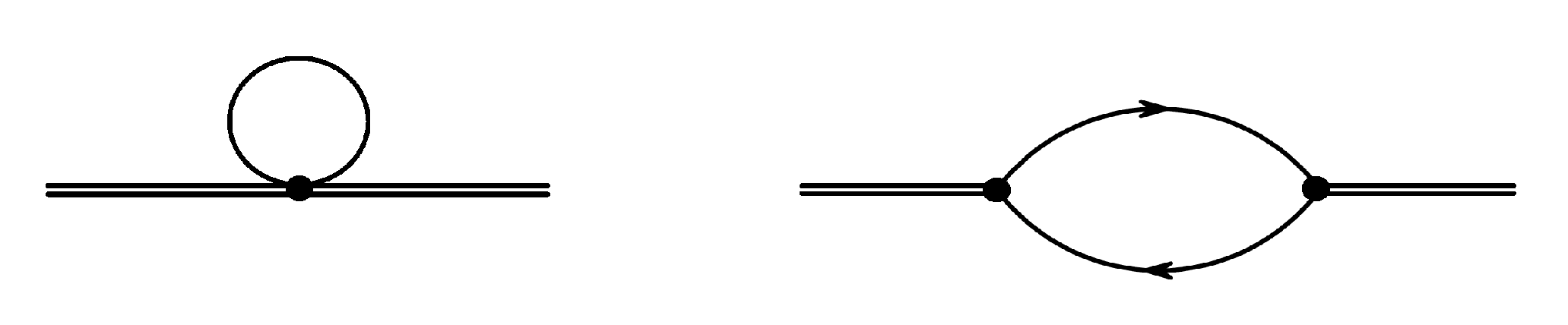
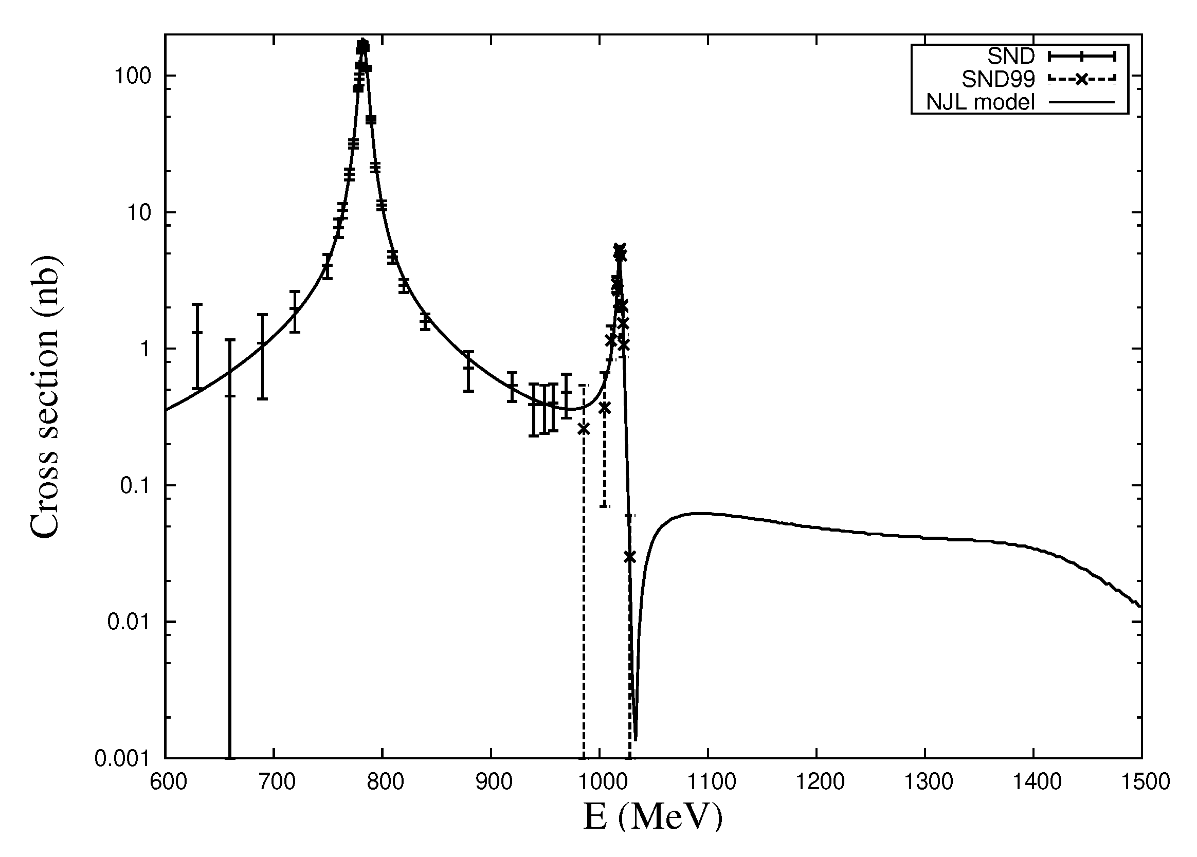
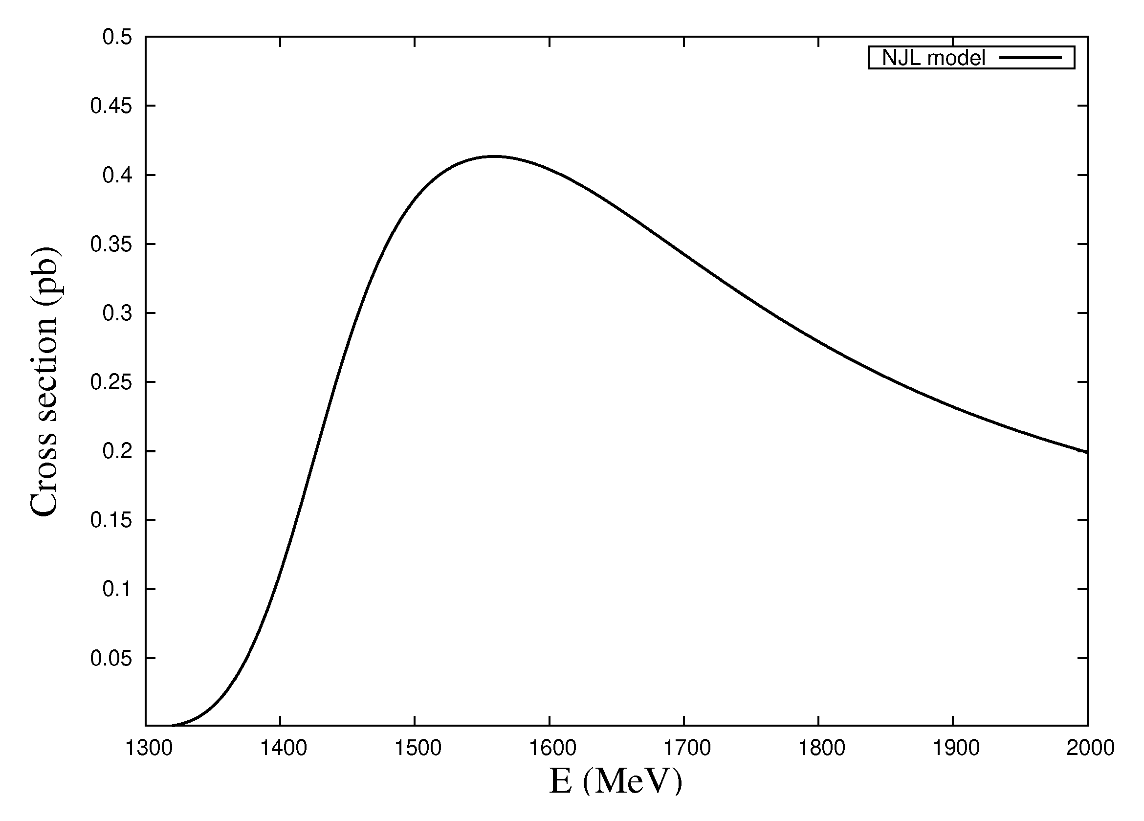
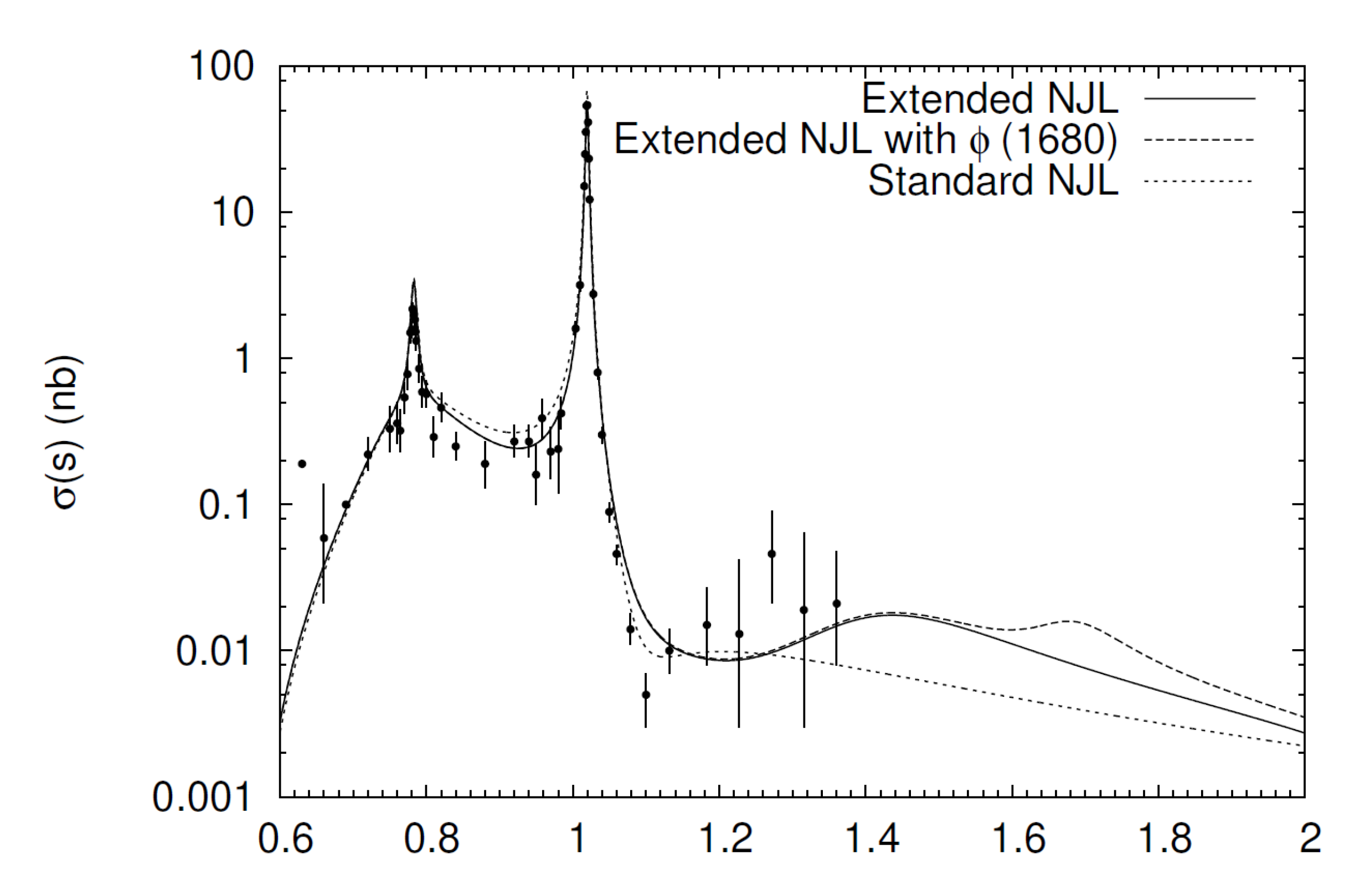
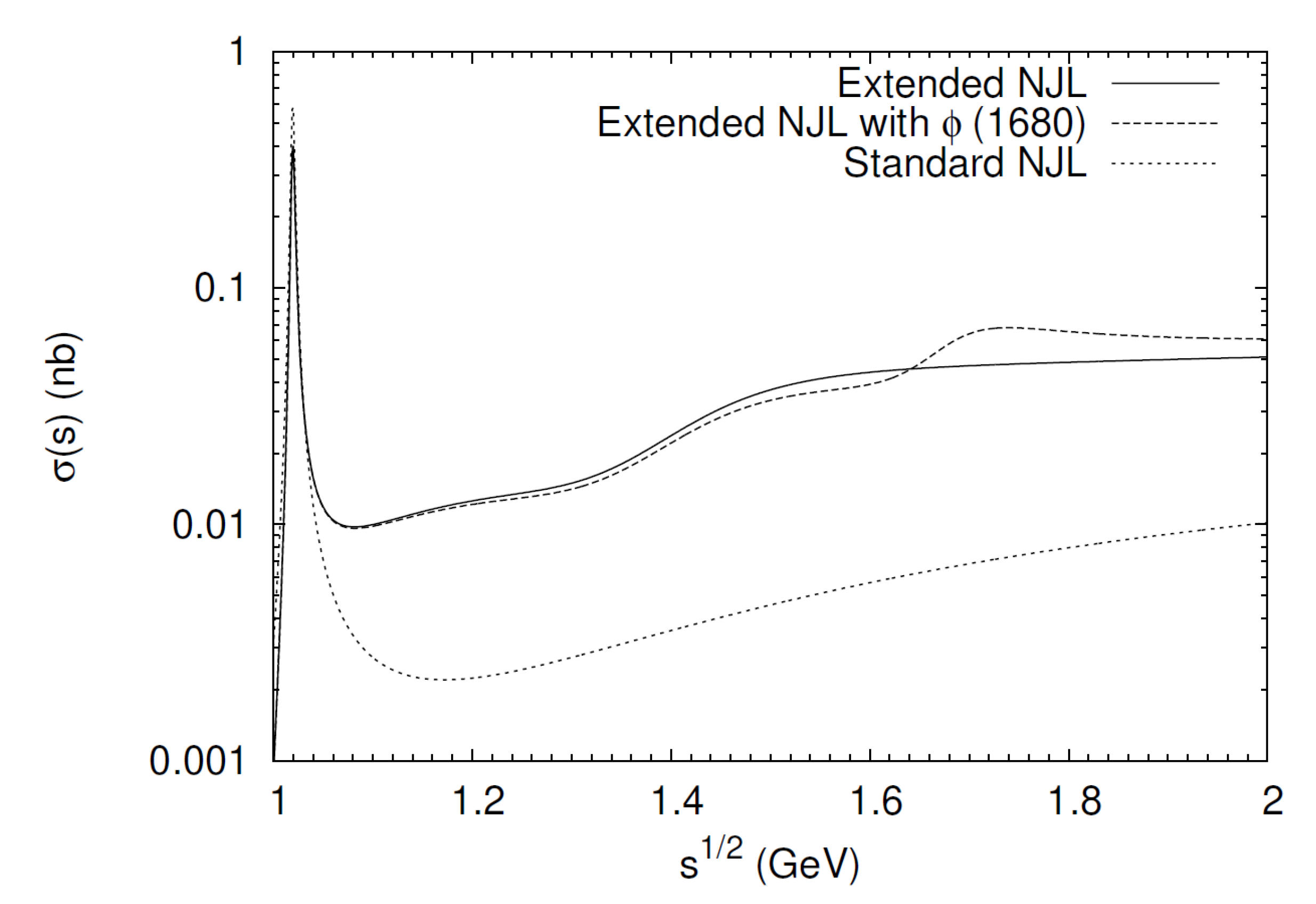
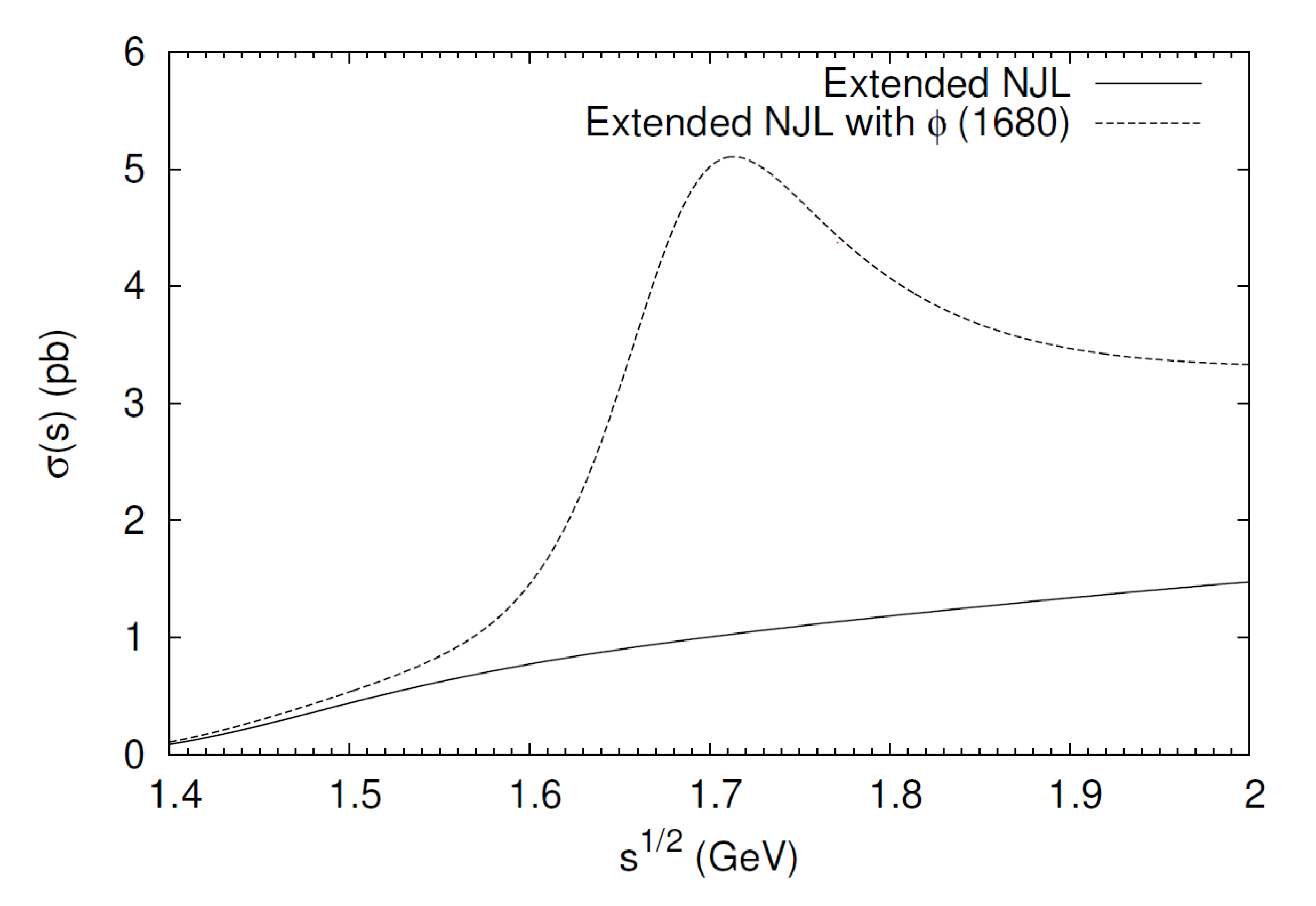
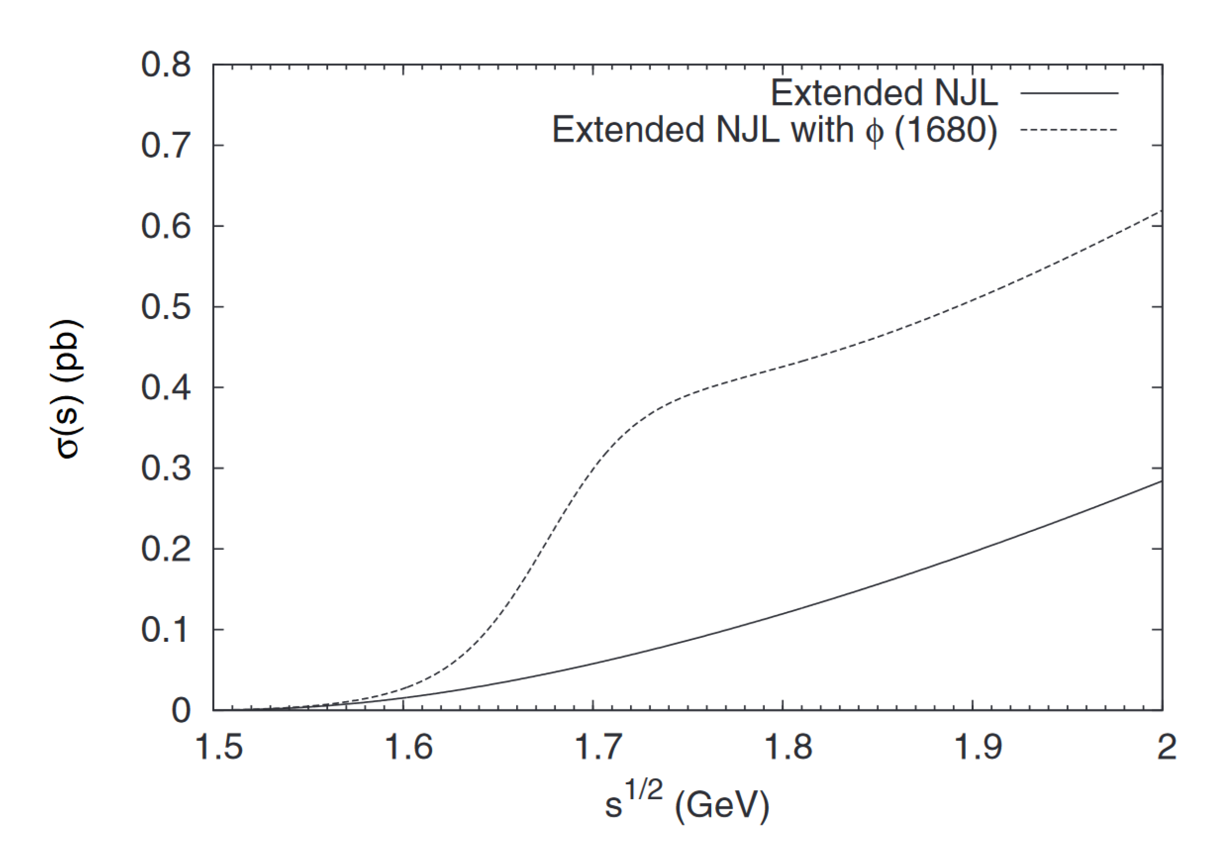
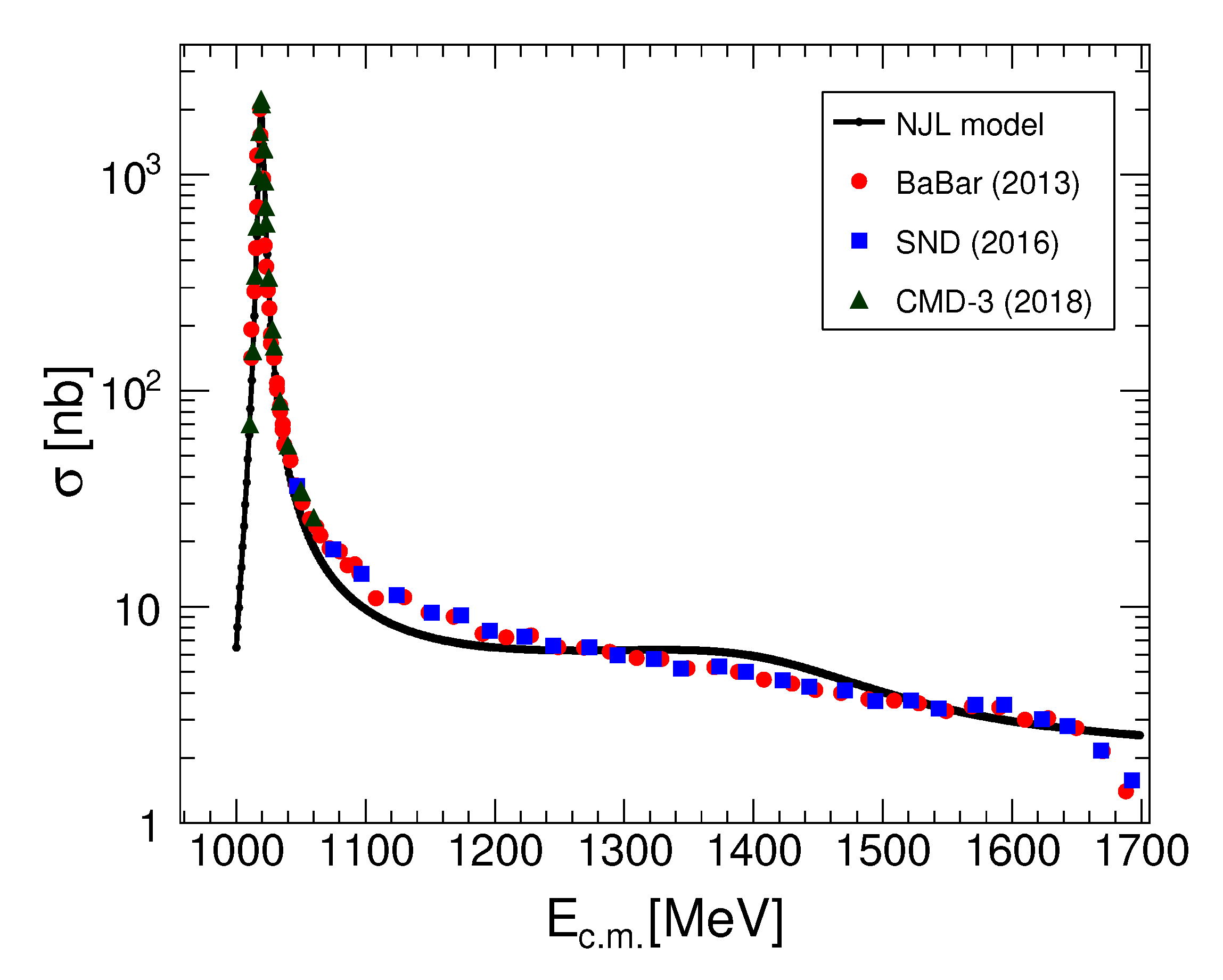
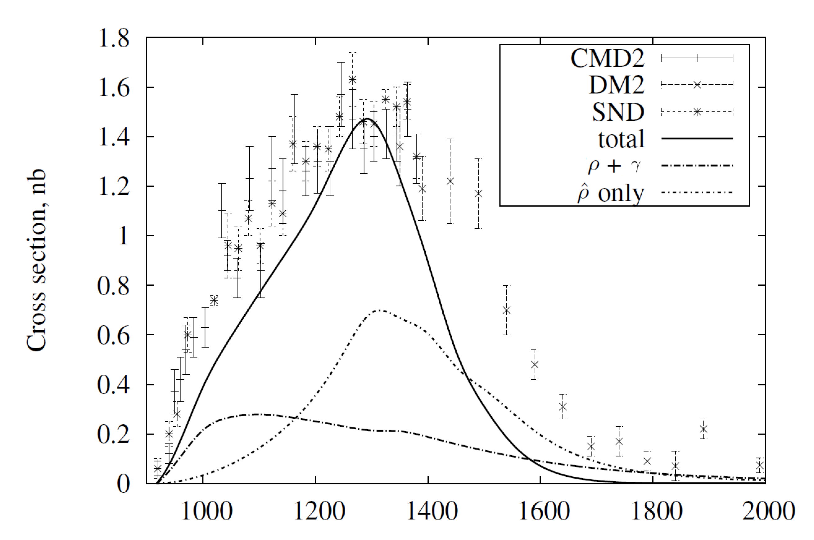
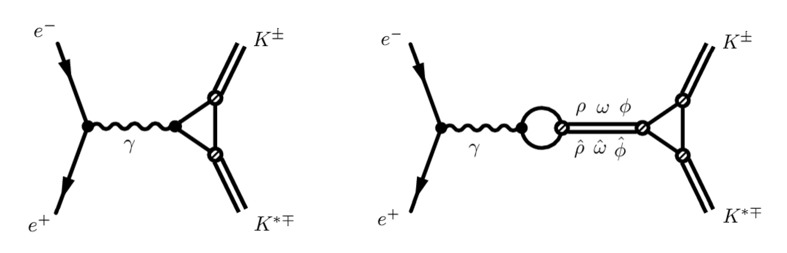
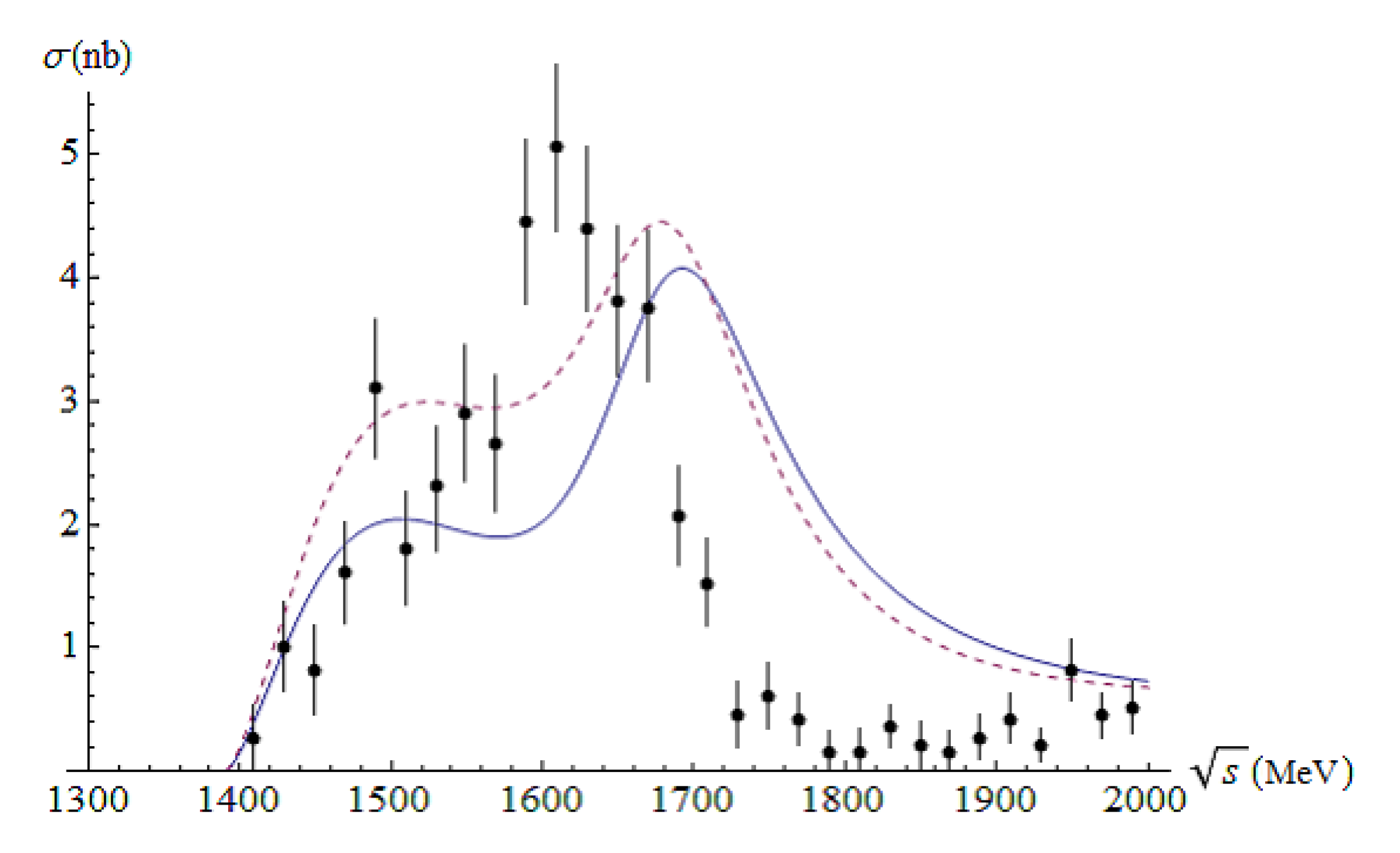
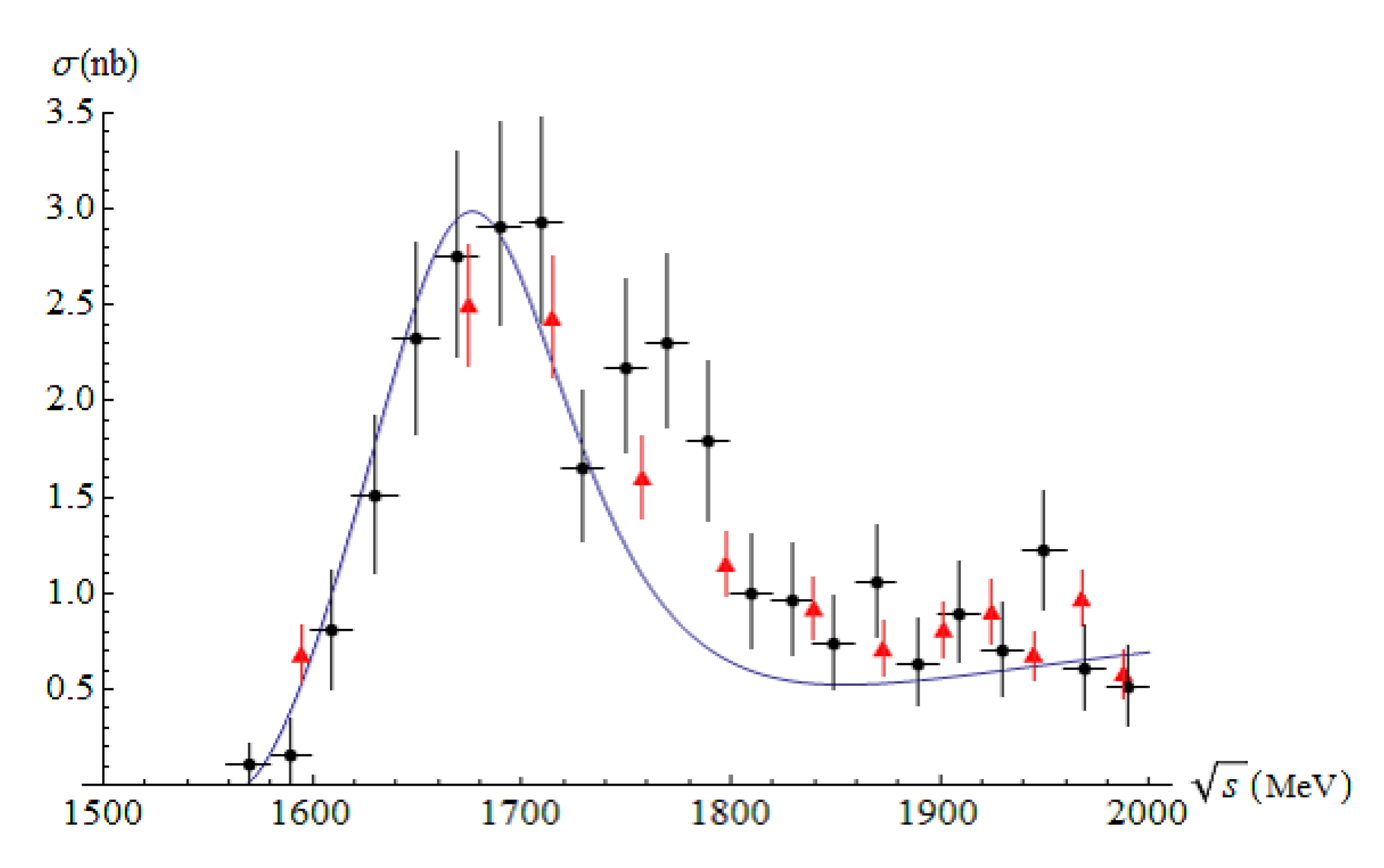
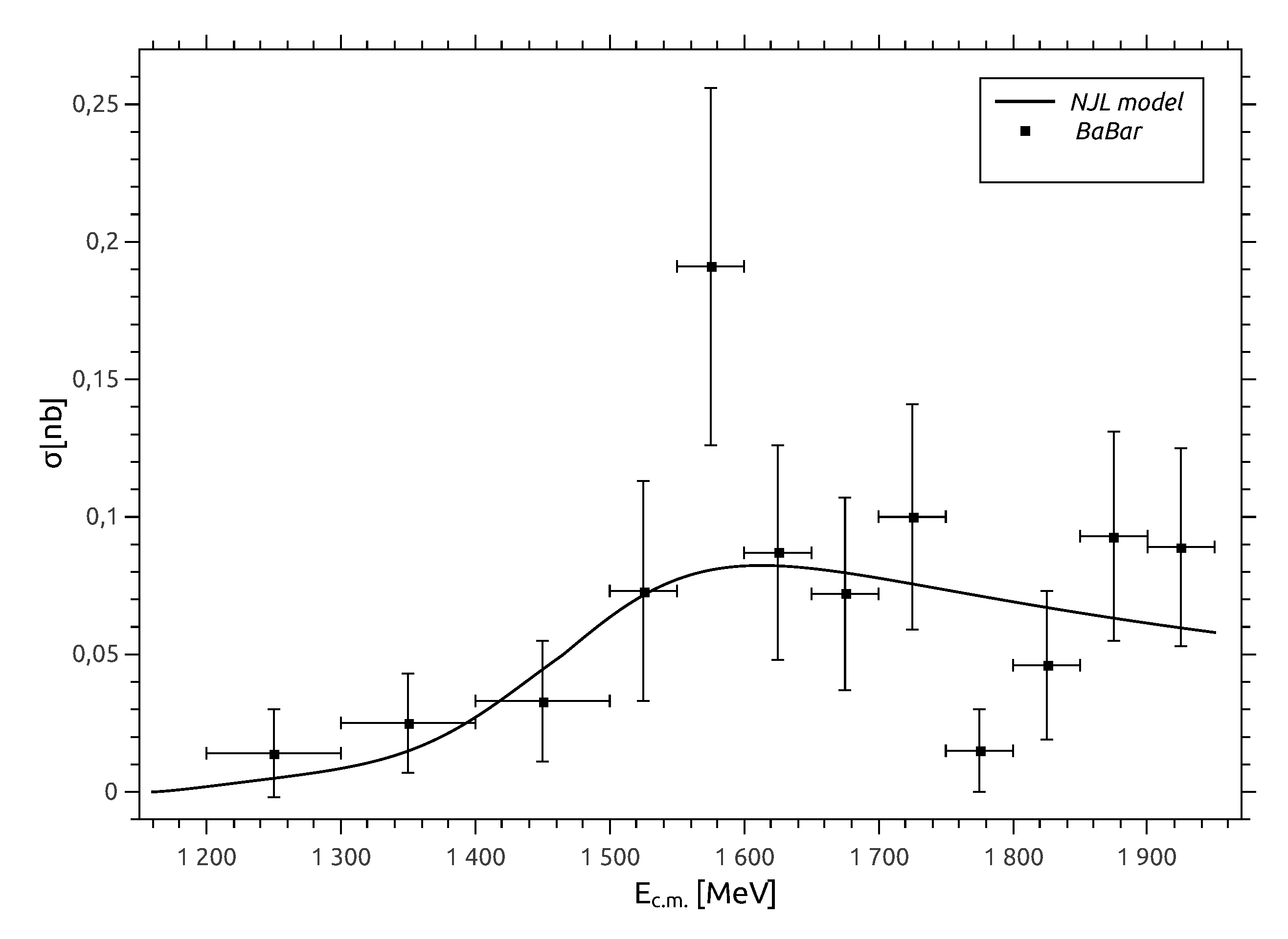
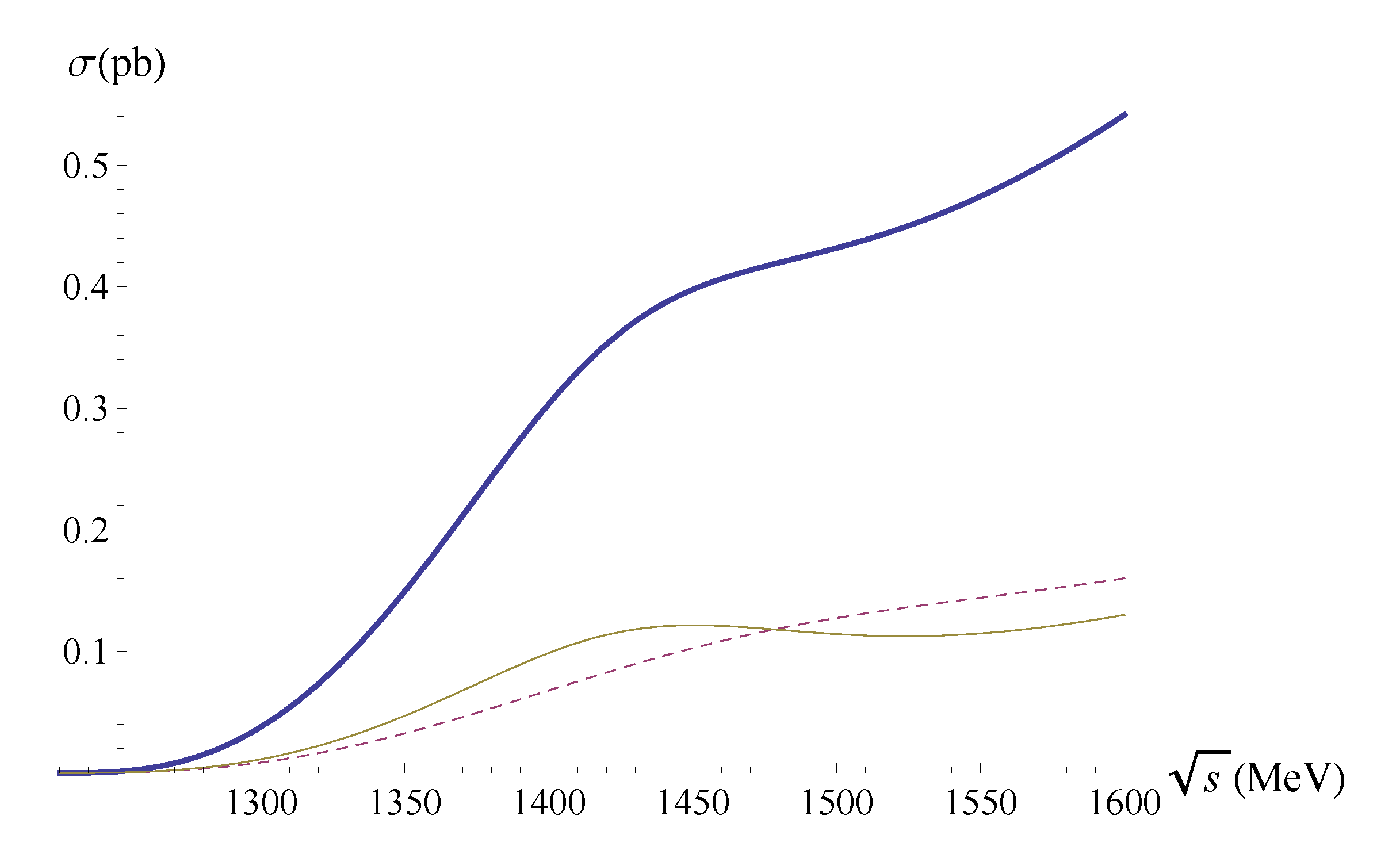
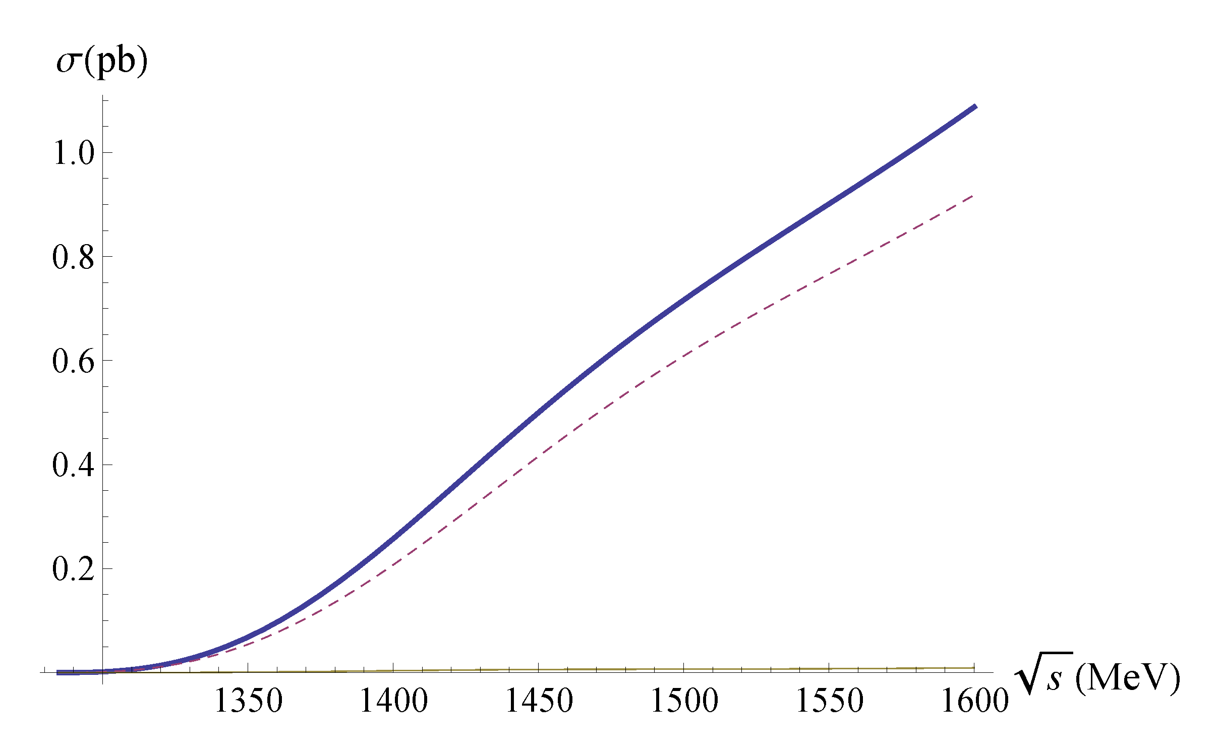
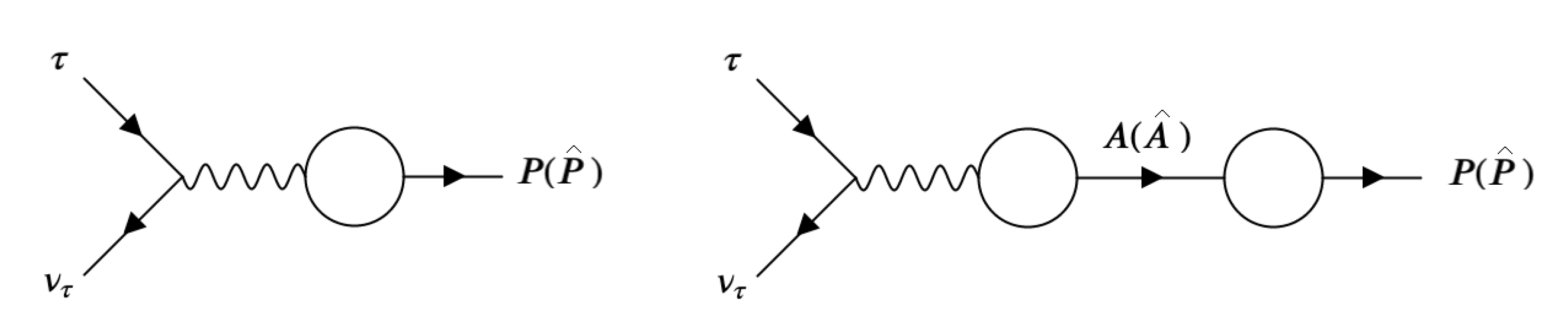
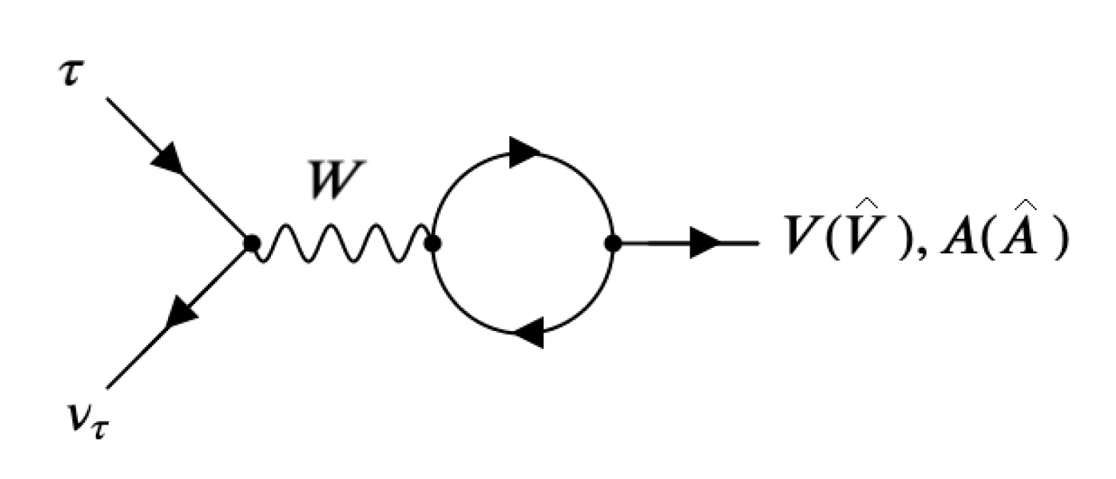
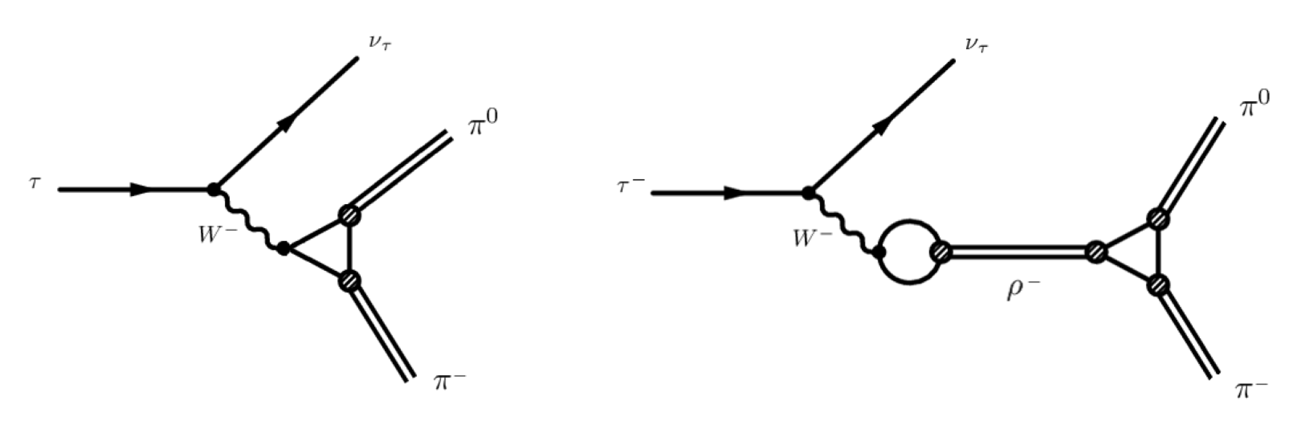
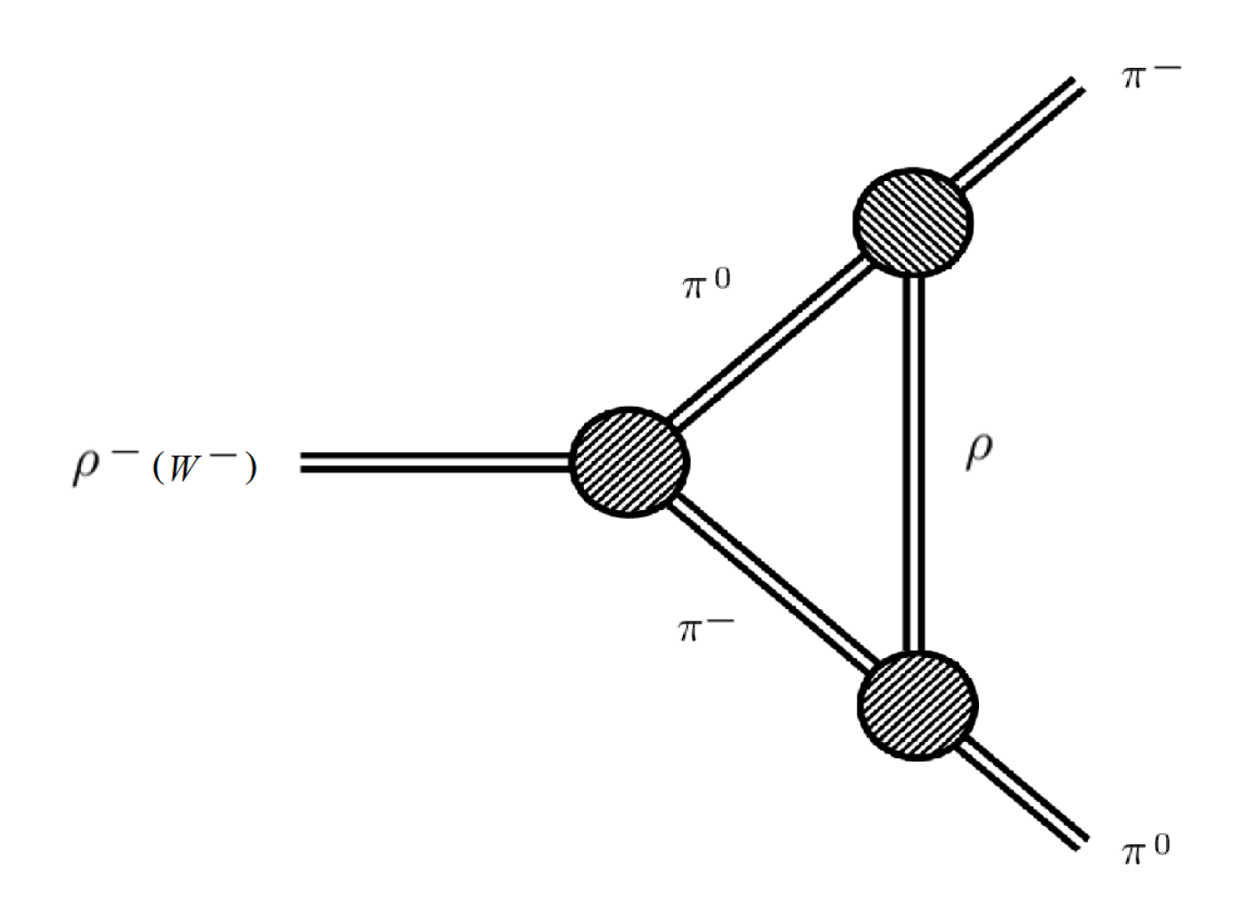
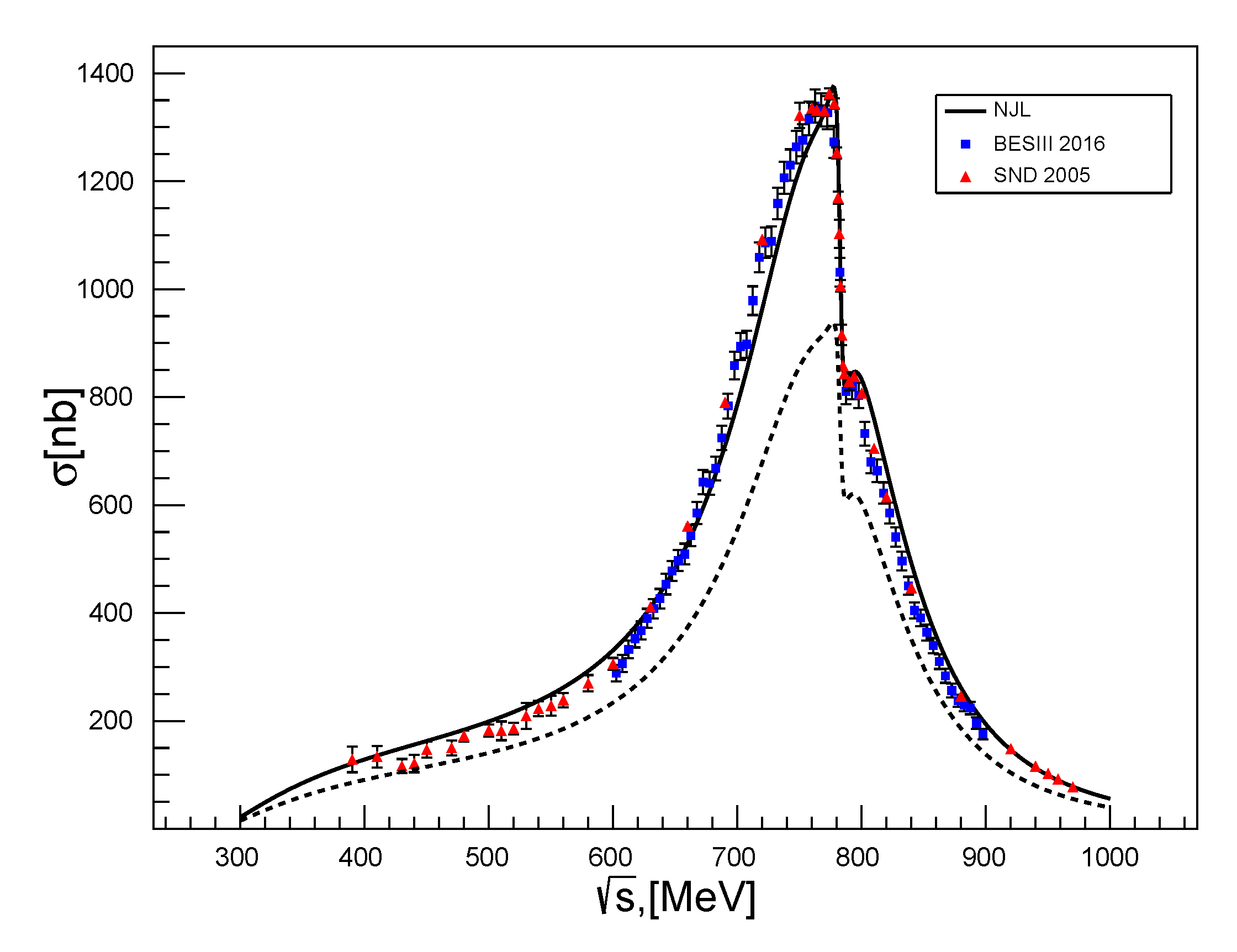
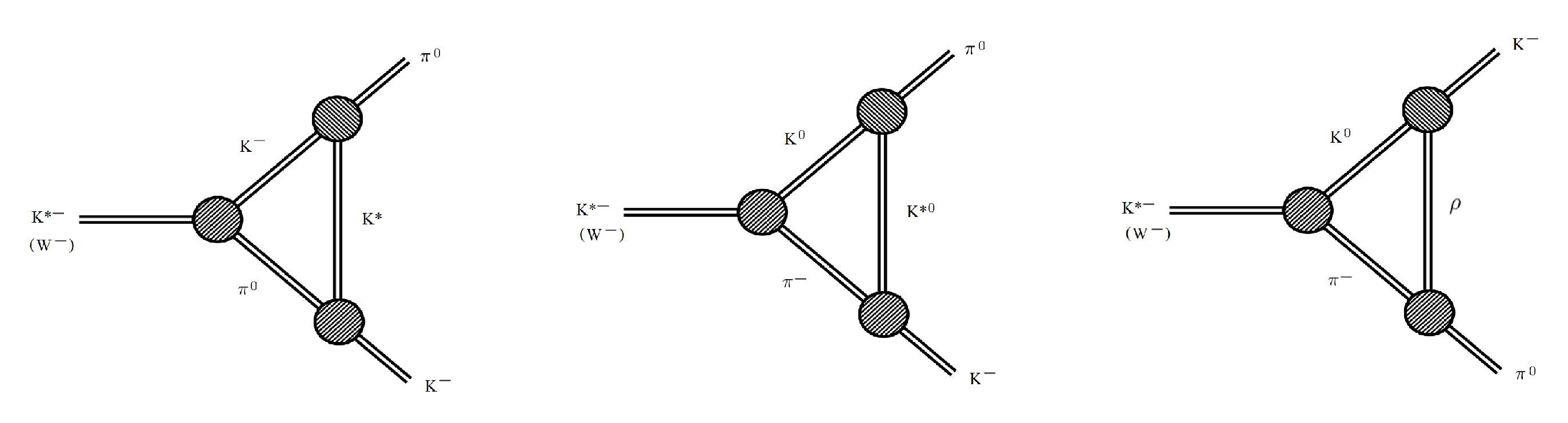
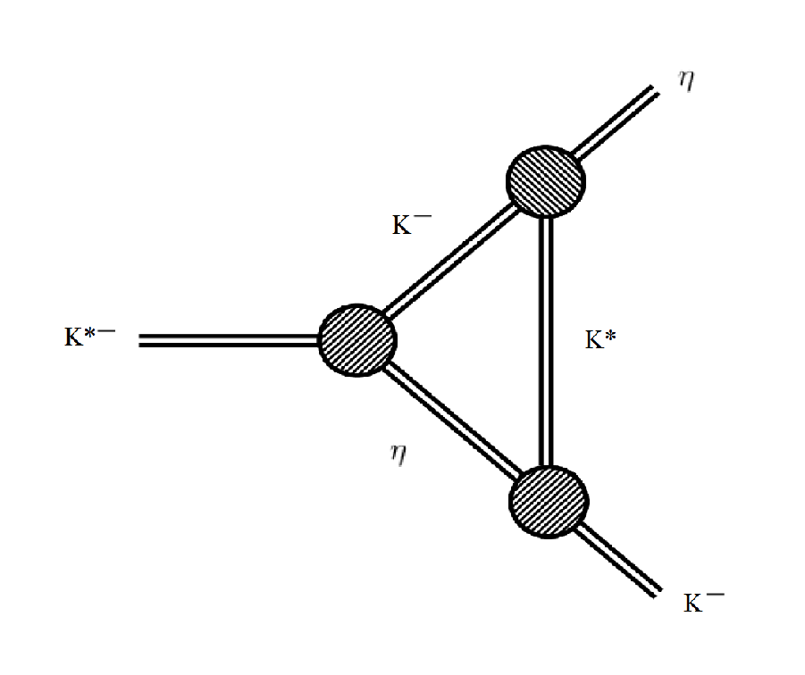
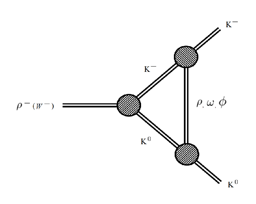
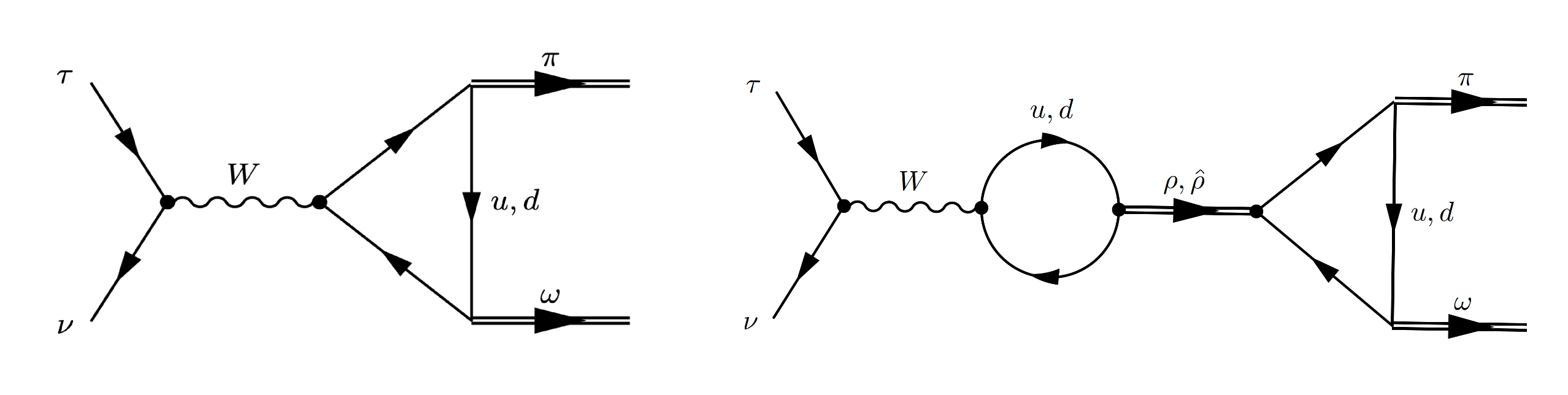
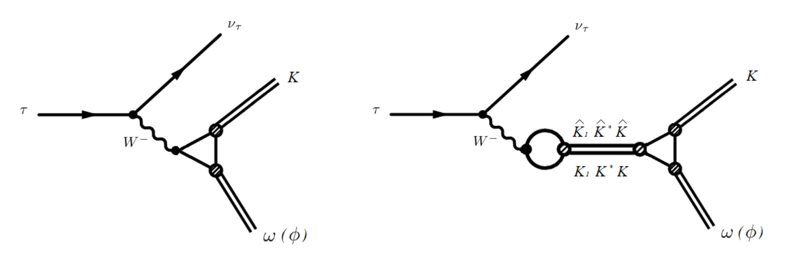
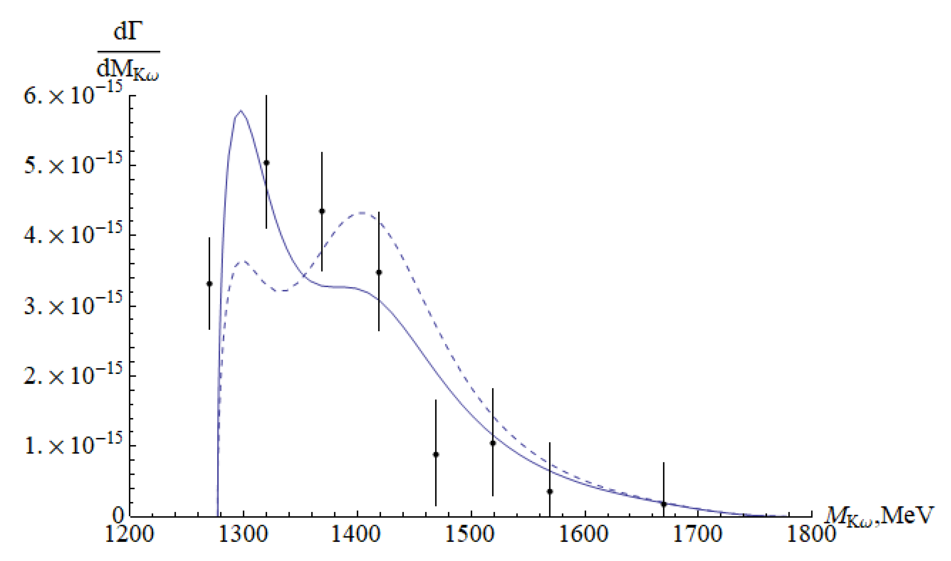
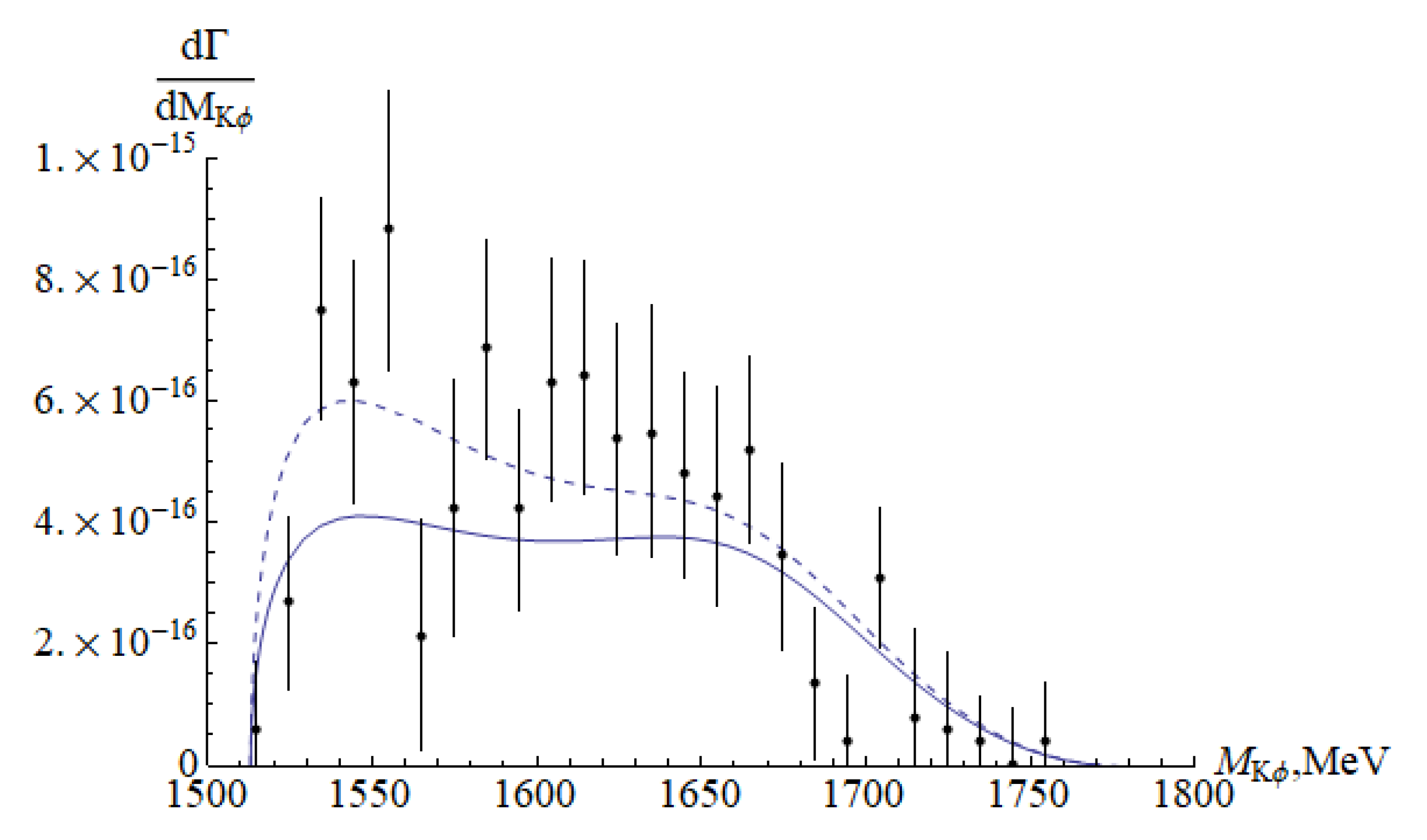
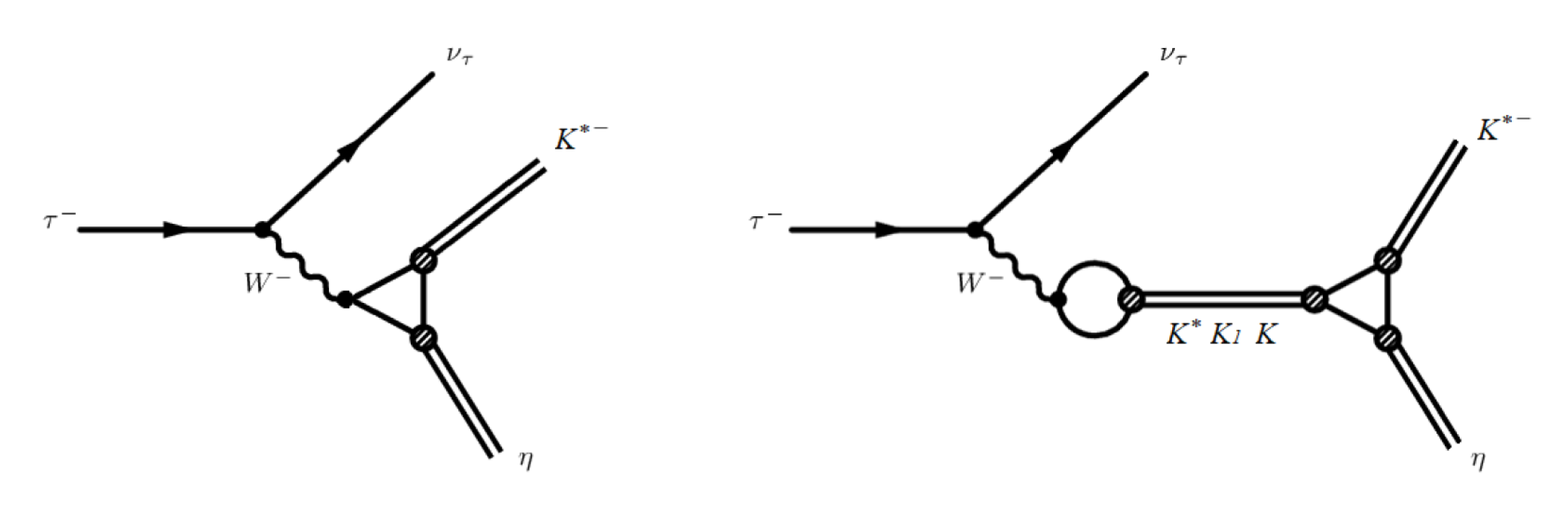
Table 1.
Mixing parameters of mesons.
| 0.71 | 0.62 | −0.32 | 0.56 | |
| 0.11 | −0.87 | −0.48 | −0.54 | |
| 0.62 | 0.19 | 0.56 | −0.67 | |
| 0.06 | −0.66 | 0.3 | 0.82 |
Table 2.
Strong decay widths calculated in the extended NJL model.
| Decays | Decay Width in the Extended NJL Model, MeV | Experiment, MeV |
|---|---|---|
| 220 | 200–600 [29] | |
| 22 | – | |
| 75 | 52–78 [40] | |
| 225 | [40] | |
| 90 | <95.52 [29] | |
| 20 | [29] | |
| 90 | ∼109 [29] | |
| 50 | ∼34 [29] | |
| 90 | – | |
| 10 | – |
Table 3.
The predictions of the extended NJL model for radiative decay widths.
| 1.43 keV | 0.33 keV | |
| 0.07 keV | 1.63 keV |
Table 4.
Predictions of the extended NJL model for decay widths and weak constants.
| Decay | Decay Width in the Extended NJL Model, MeV | ||
|---|---|---|---|
| 100 | 116 | ||
Table 5.
Predictions of the extended NJL model for lepton decays into vector and axial vector mesons.
Table 5.
Predictions of the extended NJL model for lepton decays into vector and axial vector mesons.
| Decay | Decay Width in the NJL Model, MeV | Experiment PDG [29], MeV |
|---|---|---|
| – | ||
| – | ||
| – | ||
| – | ||
| – |
Table 6.
Predictions of the extended NJL model for the branching fractions of . The contributions of different channels are given with different lines. The lines and correspond to the axial-vector and vector parts of the contact channel. The Ground line contains the summed results of all channels with intermediate mesons in the ground state and contact channel. The Excited line contains the results for the contributions of all excited intermediate mesons.
| Br () | ||||
|---|---|---|---|---|
| 0.54 | 0.52 | 2.02 | 1.97 | |
| A | 4.73 | 4.47 | 7.49 | 8.59 |
| + A | 3.08 | 3.27 | 2.12 | 2.94 |
| 0.66 | 0.64 | 0.84 | 0.82 | |
| V | 1.99 | 1.94 | 0.89 | 0.86 |
| + V | 0.37 | 0.36 | 2.6 × | 2.5 × |
| P | 0.57 | 0.53 | 0.66 | 0.61 |
| Ground | 3.83 | 3.96 | 2.57 | 3.34 |
| 5.4 × | 5.2 × | 0.74 | 0.72 | |
| 0.31 | 0.3 | 18.1 × | 17.7 × | |
| 8.6 × | 6.1 × | 1.6 × | 1.2 | |
| Excited | 0.32 | 0.31 | 0.76 | 0.74 |
| Total | 3.79 | 3.95 | 3.15 | 4.04 |
| Experiment | [29] | [29] | ||
| [109] | ||||
| [110] | ||||
Table 7.
Branching fractions of the decay .
| Channels | Br () |
|---|---|
| A | 1.21 |
| V | |
| P | 0.04 |
| Total | 1.23 |
| Experiment | [29] |
Table 8.
Predictions of the NJL model for the branching fractions of .
| Channels | Br () × | |
|---|---|---|
| A | 1.01 | 1.01 |
| V | ||
| P | 0.09 | 0.09 |
| The phase | ||
| Total | 1.99 | 1.23 |
| Experiment | [29] | |
Publisher’s Note: MDPI stays neutral with regard to jurisdictional claims in published maps and institutional affiliations. |
© 2022 by the authors. Licensee MDPI, Basel, Switzerland. This article is an open access article distributed under the terms and conditions of the Creative Commons Attribution (CC BY) license (https://creativecommons.org/licenses/by/4.0/).
Share and Cite
MDPI and ACS Style
Volkov, M.K.; Pivovarov, A.A.; Nurlan, K. Low-Energy Interactions of Mesons with Participation of the First Radially Excited States in U(3) × U(3) NJL Model. Symmetry 2022, 14, 308. https://doi.org/10.3390/sym14020308
AMA Style
Volkov MK, Pivovarov AA, Nurlan K. Low-Energy Interactions of Mesons with Participation of the First Radially Excited States in U(3) × U(3) NJL Model. Symmetry. 2022; 14(2):308. https://doi.org/10.3390/sym14020308
Chicago/Turabian StyleVolkov, Mikhail Konstantinovich, Aleksey Aleksandrovich Pivovarov, and Kanat Nurlan. 2022. "Low-Energy Interactions of Mesons with Participation of the First Radially Excited States in U(3) × U(3) NJL Model" Symmetry 14, no. 2: 308. https://doi.org/10.3390/sym14020308
Note that from the first issue of 2016, this journal uses article numbers instead of page numbers. See further details here.