
The Cosmological Constant as Event Horizon


1
Institute of Space Sciences (ICE, CSIC), 08193 Barcelona, Spain
2
Institut d Estudis Espacials de Catalunya (IEEC), 08034 Barcelona, Spain
Symmetry 2022, 14(2), 300; https://doi.org/10.3390/sym14020300
Submission received: 23 December 2021
/
Revised: 10 January 2022
/
Accepted: 28 January 2022
/
Published: 1 February 2022
(This article belongs to the Special Issue Fundamental Constants in Cosmology)
Abstract
:General Relativity allows for a cosmological constant () which has inspired models of cosmic Inflation and Dark Energy. We show instead that corresponds to an event horizon: a causal boundary term in the action. Our Universe is expanding inside its Schwarzschild radius , which could have originated from a uniform free falling cloud of mass M that collapsed as a Black Hole (BH) 25 Gyrs ago. Such a BH Universe allows for large-scale structure formation without the need of Inflation or Dark Energy.
1. Introduction
The cosmological constant has a very interesting history. For a review, see [1,2,3]. In 1917, right after the first publications of General Relativity (GR) [4], Albert Einstein applied GR to the Universe as a whole [5]. This was before the discovery of cosmic expansion [6]. Einstein realized that to account for the whole Universe, we need to include a cosmological constant, , as a new universal constant of nature. At that time, most scientists believed that the Universe has to be in static equilibrium on large scales. This is what is usually assumed for large physical systems that are allowed to evolve in isolation for a long time. However, gravity is always attractive and it is therefore hard to imagine how you can reach such an equilibrium on the largest scales where other forces are negligible. This is why Einstein had to invoke .
We can see this by considering the GR version of the Poisson equation for a perfect fluid with density and pressure p (see Equation (12) in [7]):
where is the geodesic acceleration [8]. This is also the Raychaudhuri equation for a shear-free, non-rotating fluid where and is the 4-velocity. The above equation is purely geometric: it describes the evolution in proper time of the dilatation coefficient of a bundle of nearby geodesics. Note that without , the acceleration is always negative and there is no way to reach an equilibrium, unless which is what we call Dark Energy today.
The term in the above equation is equivalent to a vacuum or a ground state of constant density (and negative pressure). It also corresponds to a centrifugal (or Hooke’s) force [9,10] in the Newtonian potential (or metric element): that opposes Newtonian gravity, . Equilibrium happens when both forces are equal, similar to the circular Kepler orbits in Newtonian dynamics.
The term was mostly abandoned after the Hubble–Lemaitre expansion law was accepted, which took some time [6]. In 1931, an unpublished manuscript of Einstein [11] considered the possibility of a Universe that expands with but remains static due to a continuous formation of matter from empty space, as in the Steady State Cosmology ([12,13]). This has the advantage of a Perfect Cosmological Principle, where the universe is homogeneous, isotropic and static. This is in better agreement with the relativity principle than the regular Cosmological Principle, which only applies to space. The key to this idea is the static deSitter (dS) metric:
where is a constant that we will identify later as in our Universe. and are the gravitational potentials of a generic metric with spherical symmetry in physical or Schwarzschild (SW) coordinates [8,14]:
where we have introduced the solid angle: .
The idea of the Steady State Cosmology solution was rejected because of the lack of observational evidence for continuous matter creation (to compensate the dilution by the expansion). However, this was a misunderstanding. There is no need for ad hoc matter creation to reconcile the observed cosmic expansion with . The frame duality [15]:
shows how the Friedmann–Lemaitre–Robertson–Walker (FLRW) in comoving coordinates (for an observer comoving with the Hubble–Lemaitre expansion law) is the same time a quasi-static Universe in the SW frame. This is similar to the dS metric but with . Under this duality, the Steady State Cosmology is not so different from the Big Bang FLRW expansion with . Indeed, our FLRW metric (to the left of Equation (4) above) asymptotically approaches the dS metric in Equation (2). As H becomes dominated by , the expansion becomes static (see also [16]) in the SW frame.
Regardless of these considerations, it turns out that we need a term again today to explain the latest measurements of cosmic accelerated expansion [17,18]. An effective term, similar to Dark Energy, might also be neeeded to understand cosmic Inflation ([19,20,21,22]). The Big Bang, Dark Energy, , Inflation and BHs are puzzles we do not yet understand at any fundamental level. Are they somehow connected? What is the meaning of the measured ?
2. The Action of GR and the Term
Consider the Einstein–Hilbert action ([8,23]):
where is the invariant volume element, is the volume of the 4D spacetime manifold, is the Ricci scalar curvature and the Lagrangian of the energy–matter content. We can obtain Einstein’s field equations (EFE) for the metric field from this action by requiring S to be stationary under arbitrary variations of the metric . The solution is ([4,8]):
where . For a perfect fluid in spherical coordinates:
where , and p are the energy–matter density and pressure. This fluid can be made of several components, each with a different equation of state . For such a perfect fluid, the solution that minimizes the action (called action on-shell ) results in a boundary term [7]:
where, in the last step, we have used the Raychaudhuri equation (Equation (1)). This is the situation when the evolution happens inside a BH. We want this boundary term to vanish (see below), so that its contribution to the action on-shell is zero: [7]. The observational fact that implies that we live inside a boundary and to cancel the boundary term we need:
which basically tells us that is just given by the matter content inside such boundary. This is similar to what happens with the event horizon of a BH. This gives an answer to the so-called coincidence problem [3]: the coincidence between the value of and matter today [7,10].
Another way to see this is to note that Equation (6) requires that boundary terms vanish (e.g., see [8,24,25]). Otherwise, we need to add a Gibbons–Hawking–York (GHY) boundary term [26,27,28] to the action:
where K is the trace of the extrinsic curvature at the boundary and h is the induced metric. We will show explicitly in Section 2.2 that the GHY boundary results in a term when the evolution happens following an FLRW metric inside an expanding BH event horizon. To cancel the GHY term, we need . That is a GHY term was first proposed in [7] and has also been later interpreted as a boundary entropy term by [29,30,31].
2.1. The Black Hole Universe (BHU) Solution
Observations show that the expansion rate today is dominated by . This indicates that the FLRW metric is inside a trapped surface , which behaves like the interior of a BH. To see this, consider the maximum distance traveled by an outgoing radial null geodesic (the Event Horizon at ,32]) in the FLRW metric:
where is the corresponding comoving scale. For small a, the value of is fixed to a constant . Thus, the physical trapped surface radius increases with time. As we approach , the Hubble rate becomes constant and freezes to a constant value . No signal from inside can reach the outside, just like in the interior of a BH. In fact, according to the Birkhoff theorem (see [33]), the metric outside should be exactly that of the SW BH in the limit of an empty outside space. So, the FLRW metric is a SW BH from the outside with . This breaks homogeneity (on scales larger than ), but this is needed if we want causality. Homogeneity is inconsistent with a causal origin.
We next look for a solution to EFE with spherical symmetry in the SW frame where we have matter and radiation inside some radius R and empty space outside:
The solution can be given in terms of the metric in Equation (3) with:
where for , we have the SW metric. At the junction , we find that:
Using Equation (4), we can immediately see that the solution is and , where is the proper time of an observer comoving with the fluid. Given and in the interior, we can find and as:
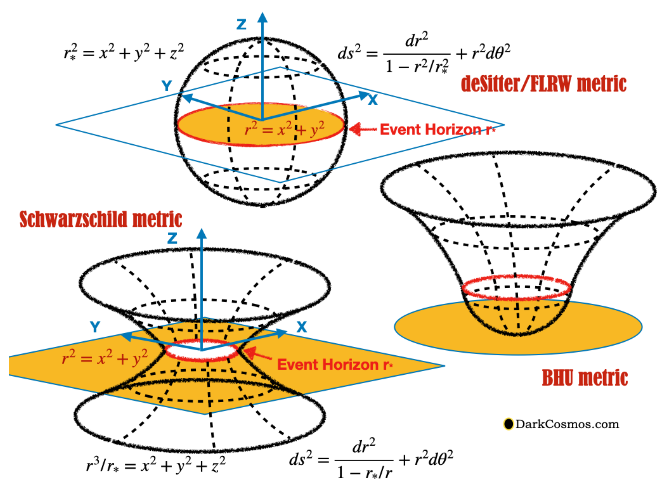
This corresponds to a homogeneous FLRW cloud of fixed mass in free-fall inside . For constant , the FLRW metric becomes the dS metric; so, the interior solution becomes Equation (2) with . Such solutions are illustrated in Figure 1.
The corresponding comoving radius to is . We can see how R can be related with a free-fall geodesic radial shell:
where . For a time-like geodesic of constant (), we have . For a null-like geodesic (), . This shows that a solution for exists for any content inside R. Israel junction conditions [34] for continuity of the metric and their derivative (the extrinsic curvature) are fulfilled for Equation (14) with no surface terms (see [15]).
Note that for (i.e., inside the BH), Equation (14) indicates that there is a region with no matter, , and a region with matter outside the Hubble horizon, . This region is dynamically frozen because the time a perturbation takes to travel that distance is larger than the expansion time [14]. The frozen region increases during collapse inside and re-enters during expansion. This is a potential source of frozen perturbations, which acts very much like Cosmic Inflation. This is illustrated by a yellow shading in Figure 2.
2.2. The GHY Boundary Term
The expansion that happens inside an isolated BH is bounded by its event horizon and we need to add the GHY boundary term to the action in Equation (10), where:
The integral is over the induced metric at , which for a time-like junction corresponds to :
So, the only remaining degrees of freedom in the action are time and the angular coordinates. We can use this metric and the trace of the extrinsic curvature at to estimate [15]. This result is also valid for a null geodesic. We then have:
The contribution to the action in Equation (10) is: where we have estimated the total 4D volume as that bounded by inside , i.e., , where the factor 2 accounts for the fact that is covered twice, first during collapse and again during expansion. Comparing the two terms, we can see that we need or, equivalently, to cancel the boundary term. In other words, the evolution inside a BH event horizon induces a term in the EFE even when there is no term to start with. Such an event horizon becomes a boundary for outgoing geodesics, i.e., expanding solutions. This provides a fundamental interpretation to the observed as a causal boundary [7,10].
3. How Emerges
We will start assuming that and show how emerges because of the dynamics inside the BH event horizon. Consider a large cloud dominated by dust ( with ) with radius R and mass M, surrounded by a region of empty space. This is a good approximation for our Universe with , which corresponds to the mass inside our future FLRW event horizon in Equation (11). The resulting BH density is very low, , which is 25% lower than the critical density today (a few protons per cubic meter).
Gravity will make such a dust cloud collapse following a free-fall time-like geodesic of Equation (14): . As there is no pressure support, it will eventually collapse into a BH when . This happened 25 Gyrs ago according to the numerical result in Figure 2. The collapse continues free-fall inside the BH as illustrated in the left half of Figure 2.
As the density inside gets larger, matter ionizes and radiation resists collapse, as it happens in stars. After 11Gyrs, the density reaches the density of a neutron star. This happens well before Planck times (Quantum Gravity). The Hubble radius at that time corresponds to a solar mass, so the situation is similar to the interior of a collapsing star. This should lead to a bounce, either because of supernova explosion or because of the elasticity of the neutron density [35]. This Big Bounce generates a hot Big Bang, similar to the bouncing of a ball on the floor.
The resulting radiation and plasma fluids cool down as they expand into the standard FLRW evolution: Nucleosynthesis and Cosmic Microwave Background (CMB) decoupling. Frozen perturbations from outside re-enter the horizon as the expansion proceeds. These are the seeds for new structure (Baryon Acoustic Oscillations or BAO and galaxies) that grow under gravitational instability. Finally, the expansion freezes (exponential inflation) as it reaches back to the original BH event horizon . As detailed in Section 2.2, the expansion inside a BH event horizon induces a term in EFE, even when there is none to start with. The expansion comes to a halt in the physical frame as nothing can come out of a BH. This provides a fundamental interpretation to the observed as causal boundary [7,10] and also for the origin of the Big Bang.
4. Discussion and Conclusions
The observed cosmic acceleration directly implies that the FLRW metric has an Event Horizon in Equation (11), which agrees well with the BHU idea [15]. Moreover, the measured cosmic density and expansion rate also match well those of a BH with and BH density . Thus, the BHU provides a fundamental explanation to the meaning and origin of the term and the hot Big Bang, as shown in Figure 2.
Inflation ([19,20,21,22]) is an important ingredient in the standard cosmological model. For a review, see [14,36]. It solves several problems, the most relevant here are: (1) the horizon problem; (2) the source of structure in the universe (such BAO); (3) the flatness problem. The horizon and structure problems arise because much of the structure that we observe today, e.g., BAO in CMB maps, was outside the Hubble horizon at the time of light emission and therefore could not have had a causal origin if there was nothing before the Big Bang. Inflation solves all these problem at the prize of introducing several new ad hoc ingredients to the early universe that are hard to test.
As shown by the yellow shaded region in Figure 2, a large fraction of the mass M that collapsed into our BHU is outside . This solves the horizon problem. The same mass outside can be the source of structure as it re-enters . Harrison [37] and Zel’dovich [38] independently proposed in 1970’s (see also [39]) that gravitational instability of regular matter alone can generate a scale-invariant spectrum of fluctuations, very similar to that produced by models of Inflation.
We have assumed here a global flat topology because this reproduces the Minkowski metric for empty space. However, the BHU solutions are also exact GR solutions for by just replacing in Equation (14). Given some energy content, EFE cannot be used to decide the topology k of the metric or the value of the effective . This is a global property that is either assumed or directly measured. So, any choice other than would require some justification that is outside GR. In that respect, we believe there is no flatness or problem within GR.
At the time of CMB last scattering, R corresponds to an angle deg. So, we can actually observe perturbations larger than R. Scales that are not causally connected! There is good observational evidence for homogeneity and lack of correlations in the CMB at (see [40] and references therein). This could be related to the so-called CMB anomalies (i.e., apparent deviations with respect to simple predictions from Cold Dark Matter, see [7,41,42] and references therein), or the apparent tensions in measurements from vastly different cosmic scales or times (e.g., [17,18,43,44]). This requires further investigation that will be presented in a separate publication.
Funding
This work has been supported by Spanish MINECO grants PGC2018-102021-B-100 and EU grants LACEGAL 734374 and EWC 776247 with ERDF funds. IEEC is funded by Generalitat de Catalunya.
Conflicts of Interest
The author declares no conflict of interest.
References
- Weinberg, S. The cosmological constant problem. Rev. Mod. Phys. 1989, 61, 1–23. [Google Scholar] [CrossRef]
- Carroll, S.M.; Press, W.H.; Turner, E.L. The cosmological constant. Annu. Rev. Astron. Astrophys. 1992, 30, 499–542. [Google Scholar] [CrossRef]
- Peebles, P.J.; Ratra, B. The cosmological constant and dark energy. Rev. Mod. Phys. 2003, 75, 559–606. [Google Scholar] [CrossRef] [Green Version]
- Einstein, A. Die Grundlage der allgemeinen Relativitätstheorie. Ann. Phys. 1916, 354, 769–822. [Google Scholar] [CrossRef] [Green Version]
- Einstein, A. Kosmologische Betrachtungen zur allgemeinen Relativitäts-Theorie. In Das Relativitätsprinzip; Vieweg+ Teubner Verlag: Wiesbaden, Germany, 1922; pp. 142–152. [Google Scholar]
- Elizalde, E. The True Story of Modern Cosmology: Origins, Main Actors and Breakthroughs; Springer Nature: Berlin/Heidelberg, Germany, 2021. [Google Scholar]
- Gaztañaga, E. The cosmological constant as a zero action boundary. Mon. Not. R. Astron. Soc. 2021, 502, 436–444. [Google Scholar] [CrossRef]
- Padmanabhan, T. Gravitation; Cambridge University Press: Cambridge, UK, 2010. [Google Scholar]
- Calder, L.; Lahav, O. Dark energy: Back to Newton? Astron. Geophys. 2008, 49, 1.13–1.18. [Google Scholar] [CrossRef]
- Gaztañaga, E. The size of our causal Universe. Mon. Not. R. Astron. Soc. 2020, 494, 2766–2772. [Google Scholar] [CrossRef] [Green Version]
- O’Raifeartaigh, C.; Mitton, S. A new perspective on steady-state cosmology. arXiv 2015, arXiv:1506.01651. [Google Scholar]
- Bondi, H.; Gold, T. The Steady-State Theory of the Expanding Universe. Mon. Not. R. Astron. Soc. 1948, 108, 252. [Google Scholar] [CrossRef]
- Hoyle, F. A New Model for the Expanding Universe. Mon. Not. R. Astron. Soc. 1948, 108, 372. [Google Scholar] [CrossRef] [Green Version]
- Dodelson, S. Modern Cosmology; Academic Press: New York, NY, USA, 2003. [Google Scholar]
- Gaztanaga, E.D. The Black Hole Universe (BHU) from a FLRW Cloud. Submitted to Physics of the Dark Universe. Available online: https://hal.archives-ouvertes.fr/hal-03344159 (accessed on 14 September 2021).
- Mitra, A. Interpretational conflicts between the static and non-static forms of the de Sitter metric. Nat. Sci. Rep. 2012, 2, 923. [Google Scholar] [CrossRef] [PubMed] [Green Version]
- Planck Collaboration. Planck 2018 results. VI. Cosmological parameters. Astron. Astrophys. 2020, 641, A6. [Google Scholar] [CrossRef] [Green Version]
- DES Collaboration. Dark Energy Survey Year 3 Results: Cosmological Constraints from Galaxy Clustering and Weak Lensing. arXiv 2021, arXiv:2105.13549. [Google Scholar]
- Starobinskiǐ, A.A. Spectrum of relict gravitational radiation and the early state of the universe. JETP Lett. 1979, 30, 682–685. [Google Scholar]
- Guth, A.H. Inflationary universe: A possible solution to the horizon and flatness problems. Phys. Rev. D 1981, 23, 347–356. [Google Scholar] [CrossRef] [Green Version]
- Linde, A.D. A new inflationary universe scenario. Phys. Lett. B 1982, 108, 389–393. [Google Scholar] [CrossRef]
- Albrecht, A.; Steinhardt, P.J. Cosmology for Grand Unified Theories with Radiatively Induced Symmetry Breaking. Phys. Rev. Lett. 1982, 48, 1220–1223. [Google Scholar] [CrossRef]
- Hilbert, D. Die Grundlage der Physick. Konigl. Gesell. D Wiss. Gött. Math.-Phys. K 1915, 3, 395–407. [Google Scholar]
- Landau, L.D.; Lifshitz, E.M. The Classical Theory of Fields; Pergamon Press: Elmsford, NY, USA, 1971. [Google Scholar]
- Carroll, S.M. Spacetime and Geometry; Cambridge University Press: Cambridge, UK, 2004. [Google Scholar]
- York, J.W. Role of Conformal Three-Geometry in the Dynamics of Gravitation. Phys. Rev. Lett. 1972, 28, 1082–1085. [Google Scholar] [CrossRef]
- Gibbons, G.W.; Hawking, S.W. Cosmological event horizons, thermodynamics, and particle creation. Phys. Rev. D 1977, 15, 2738–2751. [Google Scholar] [CrossRef] [Green Version]
- Hawking, S.W.; Horowitz, G.T. The gravitational Hamiltonian, action, entropy and surface terms. Class. Quantum Gravity 1996, 13, 1487–1498. [Google Scholar] [CrossRef] [Green Version]
- García-Bellido, J.; Espinosa-Portalés, L. Cosmic acceleration from first principles. Phys. Dark Univ. 2021, 34, 100892. [Google Scholar] [CrossRef]
- Espinosa-Portalés, L.; García-Bellido, J. Covariant formulation of non-equilibrium thermodynamics in General Relativity. Phys. Dark Universe 2021, 34, 100893. [Google Scholar] [CrossRef]
- Arjona, R.; Espinosa-Portales, L.; García-Bellido, J.; Nesseris, S. A GREAT model comparison against the cosmological constant. arXiv 2021, arXiv:2111.13083. [Google Scholar]
- Ellis, G.F.R.; Rothman, T. Lost horizons. Am. J. Phys. 1993, 61, 883–893. [Google Scholar] [CrossRef]
- Deser, S.; Franklin, J. Schwarzschild and Birkhoff a la Weyl. Am. J. Phys. 2005, 73, 261–264. [Google Scholar] [CrossRef] [Green Version]
- Israel, W. Singular hypersurfaces and thin shells in general relativity. Nuovo Cimento B Ser. 1967, 48, 463. [Google Scholar] [CrossRef] [Green Version]
- Bera, P.; Jones, D.I.; Andersson, N. Does elasticity stabilize a magnetic neutron star? MNRAS 2020, 499, 2636–2647. [Google Scholar] [CrossRef]
- Liddle, A.R. Observational tests of inflation. arXiv 1999, arXiv:astro-ph/astro-ph/9910110. [Google Scholar]
- Harrison, E.R. Fluctuations at the Threshold of Classical Cosmology. Phys. Rev. D 1970, 1, 2726–2730. [Google Scholar] [CrossRef]
- Zel’Dovich, Y.B. Reprint of 1970A&A.....5...84Z. Gravitational instability: An approximate theory for large density perturbations. Astron. Astrophys. 1970, 500, 13–18. [Google Scholar]
- Peebles, P.J.E.; Yu, J.T. Primeval Adiabatic Perturbation in an Expanding Universe. Astrophys. J. 1970, 162, 815. [Google Scholar] [CrossRef]
- Camacho, B.; Gaztañaga, E. A measurement of the scale of homogeneity in the Early Universe. arXiv 2021, arXiv:2106.14303. [Google Scholar]
- Fosalba, P.; Gaztañaga, E. Explaining cosmological anisotropy: Evidence for causal horizons from CMB data. Mon. Not. R. Astron. Soc. 2021, 504, 5840–5862. [Google Scholar] [CrossRef]
- Gaztañaga, E.; Fosalba, P. A peek outside our Universe. arXiv 2021, arXiv:2104.00521. [Google Scholar] [CrossRef]
- Riess, A.G. The expansion of the Universe is faster than expected. Nat. Rev. Phys. 2019, 2, 10–12. [Google Scholar] [CrossRef] [Green Version]
- Di Valentino, E.; Mena, O.; Pan, S.; Visinelli, L.; Yang, W.; Melchiorri, A.; Mota, D.F.; Riess, A.G.; Silk, J. In the realm of the Hubble tension-a review of solutions. Class. Quantum Gravity 2021, 38, 153001. [Google Scholar] [CrossRef]
Figure 1.
Spatial 2D polar representation of metric embedded in a 3D flat space. deSitter space (top, ) corresponds to a 2D sphere (S2) in 3D flat space. Yellow region shows the projected coverage in the true -plane. Coordinate z is an auxiliary extra dimension for illustration ( for deSitter). The true 3D space has an additional angle in , which is not shown. Schwarzschild metric (bottom left) corresponds to and the combined BHU metric is shown in the middle right.

Figure 2.
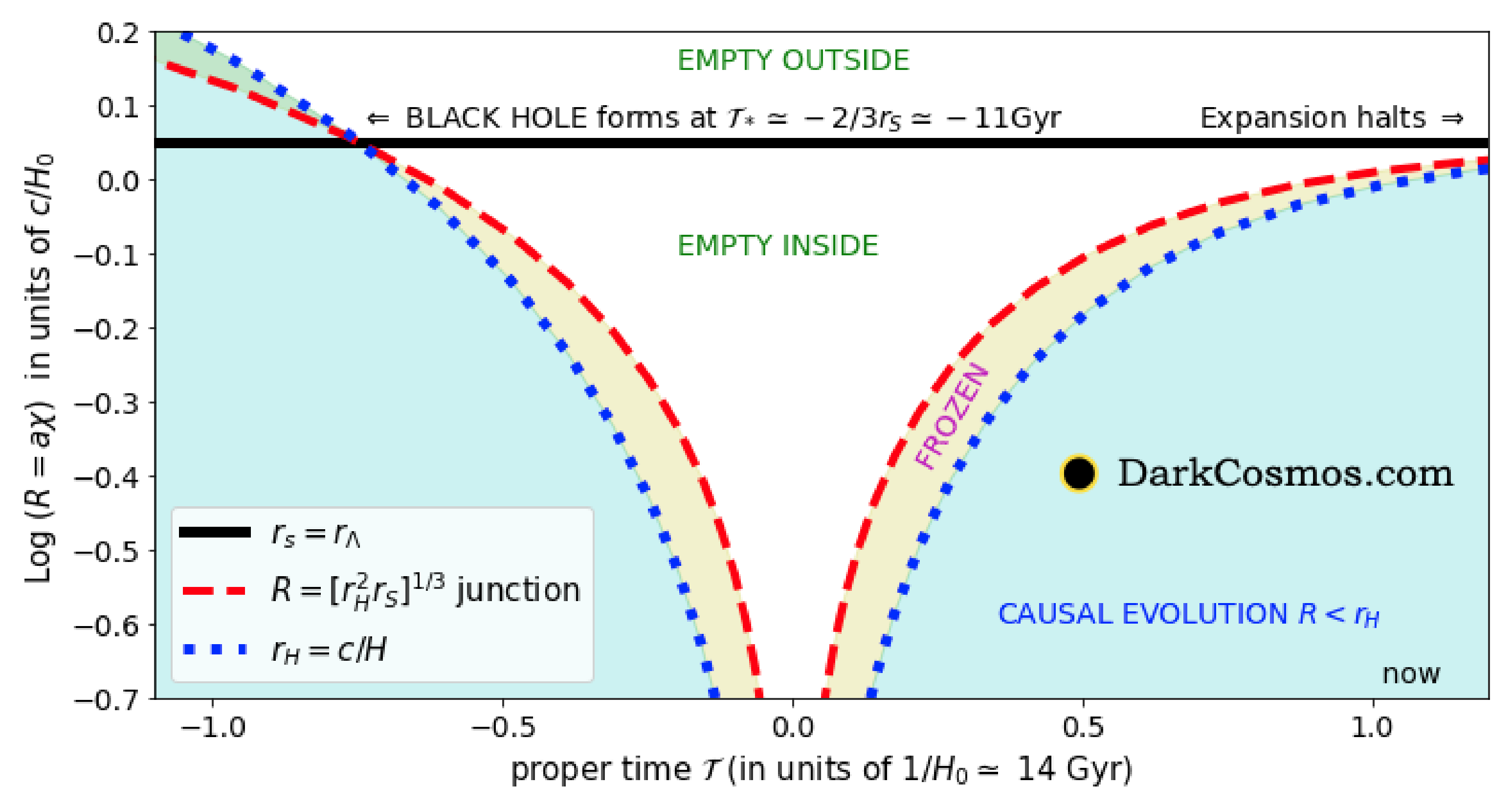
Physical radius R of a homogeneous spherical cloud as a function of proper (or comoving) time . A cloud of radius R and mass M collapses in free-fall. When it reaches , at Gyr, it becomes a BH. The collapse proceeds inside the BH until it bounces producing an expansion (the hot Big Bang). The event horizon behaves like a cosmological constant with so that the expansion freezes before it reaches back to . The calculation corresponds to with . Structure in between R and is frozen (yellow shading) and seeds structure formation in our Universe, which could include smaller BHUs, CMB, stars and galaxies. Blue shading indicates causal evolution ().
Figure 2.
Physical radius R of a homogeneous spherical cloud as a function of proper (or comoving) time . A cloud of radius R and mass M collapses in free-fall. When it reaches , at Gyr, it becomes a BH. The collapse proceeds inside the BH until it bounces producing an expansion (the hot Big Bang). The event horizon behaves like a cosmological constant with so that the expansion freezes before it reaches back to . The calculation corresponds to with . Structure in between R and is frozen (yellow shading) and seeds structure formation in our Universe, which could include smaller BHUs, CMB, stars and galaxies. Blue shading indicates causal evolution ().

Publisher’s Note: MDPI stays neutral with regard to jurisdictional claims in published maps and institutional affiliations. |
© 2022 by the author. Licensee MDPI, Basel, Switzerland. This article is an open access article distributed under the terms and conditions of the Creative Commons Attribution (CC BY) license (https://creativecommons.org/licenses/by/4.0/).
Share and Cite
MDPI and ACS Style
Gaztanaga, E. The Cosmological Constant as Event Horizon. Symmetry 2022, 14, 300. https://doi.org/10.3390/sym14020300
AMA Style
Gaztanaga E. The Cosmological Constant as Event Horizon. Symmetry. 2022; 14(2):300. https://doi.org/10.3390/sym14020300
Chicago/Turabian StyleGaztanaga, Enrique. 2022. "The Cosmological Constant as Event Horizon" Symmetry 14, no. 2: 300. https://doi.org/10.3390/sym14020300
Note that from the first issue of 2016, this journal uses article numbers instead of page numbers. See further details here.