A Proposal for a Novel Formulation Based on the Hyperbolic Cattaneo’s Equation to Describe the Mechano-Transduction Process Occurring in Bone Remodeling

Abstract

In this paper, we propose a model for the mechanical stimulus involved in the process of bone remodeling together with its evolution over time. Accumulated evidence suggests that bone remodeling could be interpreted as a feedback control process in which the mechanical state of the bone tissue is monitored, then appropriate signals are derived from the daily mechanical usage of the bone, these signals are transmitted into the surrounding region, and then they are detected by other agents whose purpose is to adapt the bone mass to the mechanical requirements of the environment. Therefore, we employ the diffusion equation for mass transport which is improved with Cattaneo’s correction to model the stimulus. This last improvement considers the effects of relaxation and non-locality, which we believe play essential roles in signaling messengers transport phenomena and are essential to match the evidence that suggests time-dependent excitations provide a more significant response at specific frequencies. To illustrate this particular behavior, numerical simulations have been performed in a 2D framework. The results fit the central aspect addressed, related to the dependency of the time of the adaptive process of bone, suggesting that our model is promising and deserves further investigation, both theoretical and experimental.

1. Introduction

The process that reshapes and leads to the mass turnover of bone tissue is called bone remodeling, and is mainly induced by external mechanical excitations. The aim of this biological process is to maintain healthy and tough tissue that is capable of sustaining the weight of the body, providing leverage for its mobility, and protecting vital organs. Specifically, by the resorption of old deteriorated tissue and synthesis of new bone material, it is possible to eliminate defects and micro-cracks as well as reorganize the mass distribution and possibly alter mechanical properties to satisfy the requirements for bone functionality. Naturally, this process is also beneficial in overcoming minor injuries or traumas which are not particularly severe and extensive [1,2,3,4].

Like many biological processes, bone remodeling can be described as a feedback control loop, where the role of adjusting the mechanical response of bone is allocated to specific bone cells. Osteocytes are responsible for acquiring information about the mechanical state of the tissue; therefore, they can be regarded as a distributed sensor network. Osteoclasts and osteoblasts are instead responsible for the change of solid inorganic mass by resorbing and producing it, respectively. In particular, since osteocytes can neither synthesize nor resorb bone tissue, it is widely acknowledged that they organize bone remodeling in response to mechanical stimulation by coordinating the actions of osteoblasts and osteoclasts residing on the inner bone surface (made available by porosity). A crucial aspect for comprehending this process is, therefore, the ways and the paths used by those cells to interact in order to fulfil their duties. In this context, the most straightforward mechanism of cellular communication could be assumed to be paracrine signaling. Namely, the mechanically stimulated osteocytes secrete into the immediate extracellular environment chemical messengers, also called paracrine factors, such as proteins/peptides, which act in a hormone-like fashion [5]. These signaling molecules travel by means of diffusion over a relatively short distance towards the nearby actor cells. The gradient of factors received determines the outcome of the remodeling process, altering those cells’ behavior. The receiving cells have appropriate receptors available on their membrane to receive the incoming signals and successfully adapt their response. We remark that this can be assumed as a primary path of cell signaling; however, the actual mechanisms involved in the remodeling process are much more complex. Indeed, it is also possible to consider ulterior communicating paths among osteoblasts, osteocytes, and between osteoblasts and osteoclasts. For the sake of completeness, we note that as opposed to paracrine cell signaling, when signaling factors influence the behavior of cells of the same kind this is referred to as autocrine cell signalling. Since the discussion of these biological mechanisms is beyond the purview of this paper, we focus our modeling experiment only on the primary mode of cellular communication from osteocytes to the cells acting in the mechanically adaptive process of bone (osteoblasts and osteoclasts), while neglecting those effects that we believe have a lower impact.

Following Frost’s approach [6], we employ a feedback model based on a variable called stimulus, which is representative of the mechanical state of the bone. The key idea here is that there is a reference stimulus associated with the homeostatic condition, representing an ideal state of deformation and, thus, a set point for the mechanical properties of the bone. Every external mechanical stimulation induces an actual stimulus. The difference between these two levels of the stimulus, i.e., the acquired and the homeostatic one, determines the responses of resorption or synthesis which intends to make the tissue more compliant or stiffer by changing the mass density correspondingly, in response to the mechanical demands of the environment. In other words, the stimulus is a conceptual, comprehensive way to describe the mechanical state of the bone based on some fundamental mechanical quantities such as, for instance, the deformation energy density (see, e.g., [7,8,9]). In view of the fact that the mechanical state acquired by osteocytes can be summarized by the stimulus, and the principal path for the transmission of the information brought by it is entrusted to paracrine factors, which are released and spread via diffusion, we reasonably assume a diffusive model for the stimulus to describe this type of signal transference [10]. This perspective allows us to retain the non-local nature of the stimulus [11]. Herein, for non-local behavior, we note that the response to a stimulus at a given point cannot be determined solely from the value of the stimulus at that exact point; however, this depends on what happens in an entire region surrounding the point within a specific range of action. This means that bone remodeling carried out by the actor cells at a given point is influenced by the signals collected by all the osteocytes in the vicinity within a specific spatial horizon. Indeed, in the literature, the stimulus is sometimes defined as a convolution integral for this purpose [1,12].

The mechanical excitation which the bone is typically subjected to can be static or dynamic. Many experimental studies proved that time-variable loads are the most effective in bone remodeling [13,14,15,16,17]. In response to static loads, instead, the tissue becomes accustomed after a while, and the process becomes increasingly less responsive. This behavior is not surprising at all since, during everyday activities, the skeleton is subjected to a few loads of both high amplitude and low frequency (around 2000–3000 microstrains, 1–3 Hz) and a multitude of excitations with small amplitudes but with larger frequencies (less than 500 microstrains, 10–60 Hz) [18]. The former loads are due to activities such as walking or running; the latter loads are due to postural muscle contractions. Naturally, the time of exposure to such loads, as well as the duration of rest between subsequent loading cycles, or the frequency of these loading–unloading cycles (presumably with a day of activity and a night of inactivity) are also influential aspects in determining the overall bone adaptive process [19].

The dependence of remodeling on the time variability of the external mechanical loads is a crucial factor in modeling the process. In the literature, this aspect is directly incorporated into the definition of the stimulus, making it proportionally dependent on the load frequency [20] or the deformation rate [21]. This last choice is particularly attractive because it can be explained from a mechanical point of view. Indeed, the deformation rate is linked to energy dissipation [12,22]; therefore, it is associated with the damping properties of bone tissue, which play a role in its mechanical function.

However, even though this dependence could be considered to explain some aspects of the phenomenon, it overlooks the critical feature that remodeling exhibits: there are some frequencies that benefit the process. For this reason, some clinical therapies are based on whole-body excitation with vibrations in a specific frequency range. On the contrary, in the actual available models, the more the frequency increases, the more that bone growth is favored.

A possible way to describe such a selective dependence on frequency could be via a mechanical resonance. Unfortunately, this possibility is quite improbable due to the following reasons: (1) the natural frequencies of bones (they are typically greater than 100 Hz) do not fit with the frequencies typically used in clinical therapies (10–60 Hz); and (2) a mechanical excitation in resonance could destroy the bone instead of stimulating its growth.

In this paper, we propose a possible way to incorporate this fundamental aspect related to the effect of the time variability of the loads into the model. Our proposal consists of generalizing the diffusion equation for the stimulus with the hyperbolic Cattaneo’s equation [23] (see for more details also [24,25]). In fact, Cattaneo’s equation may provide both the stimulus signal’s diffusive nature and the possibility of wave propagation with some kind of dissipation.

This paper is organized as follows: first, in Section 2, we introduce the proposed model for the mechanical stimulus. Then, in Section 3, we describe the employed mechanical formulation, i.e., a Biot-type continuum poroelastic model. In Section 4, we provide numerical results for a representative preliminary case. Finally, in Section 5, we draw some conclusions.

2. Modeling the Functional Adaptation of Bone

Functional adaptation in the bone can be thought to be regulated by the feedback of a mechanical stimulus in a self-organizational process that aims to optimize the mechanical response of the bone on the basis of external mechanical excitations. In a continuum context such as the one that we assume, because of the porous nature of the bone, an apparent mass density must be considered. Indeed, it is based on the perceivable volume, namely, the one confined in the outer surface of the bone, including its porous cavities. Hence, to describe the evolution of the bone tissue over time, we consider a first-order differential equation that specifies how the Lagrangian apparent bone mass density ${\rho }_{\mathrm{b}}^{*}$ adapts itself. The change of mass density is linked to the stimulus S, which describes the mechanical state of the tissue, and to the porosity $\varphi$. The role of the porosity, among other things, is to prevent the mass density from reaching negative values and growing indefinitely. Notably, resorption and synthesis of the tissue change the Lagrangian porosity and, therefore, the apparent mass density. In formulae, the evolution law for the Lagrangian apparent mass density is assumed to be as follows:

$$\frac{\partial {\rho }_{\mathrm{b}}^{*}}{\partial t}=\mathcal{A}(S,\varphi )$$

(1)

In Equation (1), the function $\mathcal{A}$ is particularized [26] as:

$$\mathcal{A}(S,\phi )=a\left(S\right)H\left(\varphi \right),$$

(2)

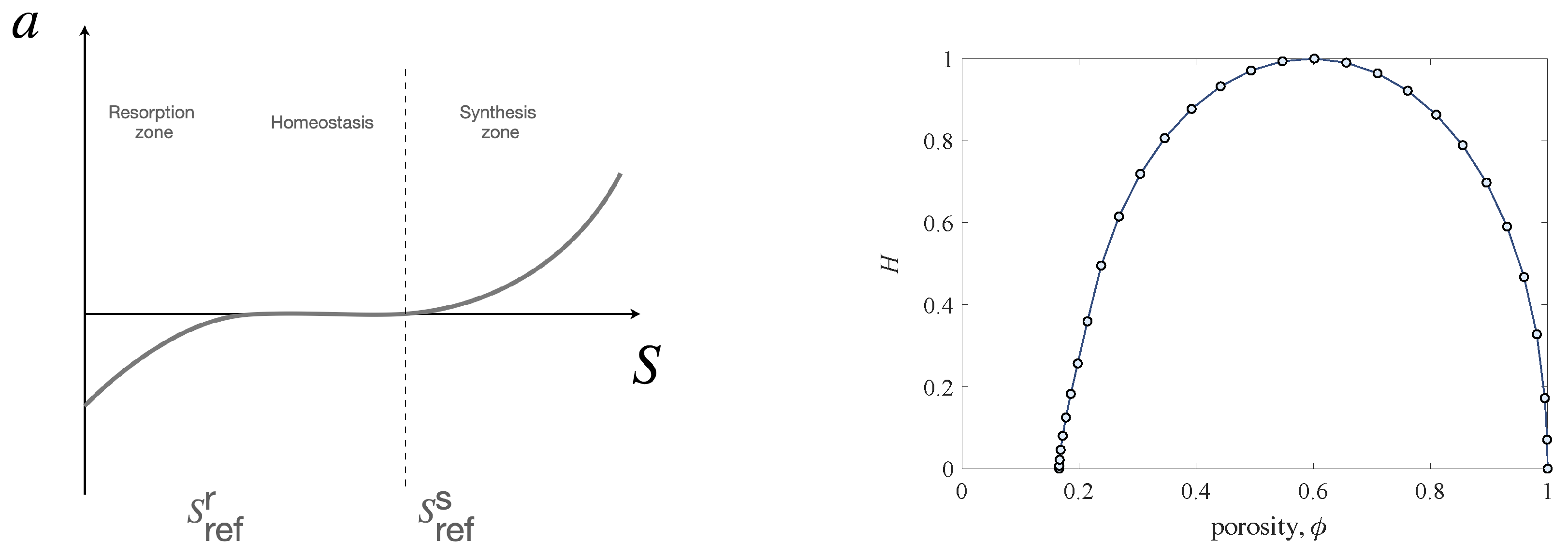
where the function $a\left(S\right)$ is specifically designed to have three different behaviors activated by the level of the stimulus (see Figure 1). When the stimulus level is insufficient (when the level of deformation is low), the osteoclasts become operative by resorbing the tissue, consequently making the bone more deformable. Indeed, the change in mass density results in a variation of the elastic moduli of the bone. After exceeding a sufficiently high stimulus level (high deformation), the osteoblasts become active with the apposition of new tissue. Indeed, in this case, the deformation is sufficiently large, and the increase in mass density has the main effect of stiffening the bone. The effect of remodeling changes the mechanical properties of the bone in order to compensate for an abnormal response due to external mechanical actions and restore a new equilibrium point, namely an optimal level of deformation, assuming the deformation as representative of the mechanical state. In these active zones, the slopes of the function $a\left(S\right)$, possibly being different, represent the synthesis and resorption rate for the given bone tissue. Between these two operational conditions, it is possible to define the homeostatic state that corresponds to an optimal state of deformation and, hence, does not require any change in the mechanical bone response. This last outcome can be obtained by setting the function $a\left(S\right)$ to zero in a given stimulus interval, which is also called the lazy zone, characterizing homeostasis. In detail, the lazy zone is defined by two thresholds $S_{\mathrm{ref}}^{\mathrm{r}}$ and $S_{\mathrm{ref}}^{\mathrm{s}}$ that also represent the two levels of stimulus beyond which resorption stops and synthesis starts, respectively.

Possible bone remodeling sites are internal surfaces left by porous voids, i.e., the inter-trabecular spaces in cancellous bone and Haversian canals in cortical bone. The osteoclasts and the osteoblasts for their regulatory task are located on these surfaces. To take into account this aspect, the specific surface function H is introduced in the model. It represents the amount of internal surface per unit volume as a function of the porosity. Its shape is heuristically estimated for an ideal cellular square lattice [27] and tends to vanish in the limiting cases when porosity tends to zero or one (see Figure 1). Indeed, in the modelling, it allows us to restrain the remodeling process when the apparent mass density reaches values that cannot be transcended. These limits physically correspond to cases in which the inner surfaces are no longer available (zero porosity) or where the empty space is too ample (porosity equal to one), resulting in a lack of support for the actor cells.

Assuming Equation (1) governs the evolution of the mass density during the remodeling process, we need to define the stimulus S and determine how it changes when responding to the demands of the environment.

Herein, we define the stimulus as a quantity that satisfies Cattaneo’s equation. The rationale behind this choice lies in the possibility of exploiting both the diffusive and the propagation characteristics of the equation, with a broad scope of factors used to better describe the considered process. The equation, was firstly proposed to eliminate the paradox of the instantaneous propagation of thermal disturbances; however, it can naturally can be applied, like many other mathematical tools, to a multitude of different applications. The model for the stimulus is then given by the following equation:

$${\tau }_0\frac{{\partial }^{2}S}{\partial t^2}+\frac{\partial S}{\partial t}=\mathrm{Div}\left(\kappa \nabla S\right)+r+s,$$

(3)

where the characteristic time ${\tau }_0$ is introduced, describing the relaxation time, namely the typical period needed for the system to return to equilibrium from a perturbed state. The parameter $\kappa$ represents the diffusion coefficient, which in the general case can be replaced by a symmetric positive definite matrix.

In fact, this formulation considers the effects of relaxation and non-locality, which we believe play essential roles in signaling messengers transport phenomena.

The other two terms in Equation (3), r and s, are the source and sink contribution, respectively. The source r defines the stimulus origin and is directly linked to the cause that determines its presence in the tissue. Conversely, the sink term s models the action of metabolic activity required to resorb the stimulus from a macroscopic point of view. At the microscopic level of cells, the chemical messengers are captured by receptors and therefore are no longer prone to diffusion or propagation. Furthermore, after being relieved of their duties, they are reabsorbed.

Specifically, we postulate that the source of the stimulus depends on the mechanical deformation (given by the strain tensor $\mathit{E}$) and, more specifically, on the strain energy density of the solid matrix, ${\mathcal{E}}_b$ (see Equation (14) for the detailed form), which can be expressed as follows:

$$r=\varpi \left({\rho }_{\mathrm{b}}^{*}\right){\mathcal{E}}_b\left(\mathit{E}\right),$$

(4)

where the function $\varpi \left({\rho }_{\mathrm{b}}^{*}\right)$ can be interpreted as a proper weight that modulates the source signal on the base of the level of stimulus that should be produced. At a cellular observation scale, this function is linked to the number of osteocytes per unit volume. It can be regarded as the performance index of the osteocyte multi-sensor network. The basic idea is that the more osteocytes there are, the better the signal reconstruction characterizing the mechanical state of the tissue is. On the contrary, a deficiency of osteocytes will result in a worse acquisition of mechanical information. At first approximation, we can assume that the number of osteocytes per unit of volume is proportional to the bone mass density since they are distributed uniformly on the solid bone matrix. Thus, we can shift the dependence on the osteocyte density towards the bone mass density, as indicated in Equation (4). Following this reasoning, clearly, the weight function $\varpi \left({\rho }_{\mathrm{b}}^{*}\right)$ is zero when the mass density vanishes, increases monotonically with increased mass density, and tends asymptotically to a constant for mass density approaching a saturation corresponding to zero porosity. A possible choice for such a function is, therefore, written as follows:

$$\varpi \left({\rho }_{\mathrm{b}}^{*}\right)=A_{oc}tanh\left(\xi {\rho }_{\mathrm{b}}^{*}\right)H_v\left({\rho }_{\mathrm{b}}^{*}\right),$$

(5)

The constants $A_{oc}$ and $\xi$ are constitutive parameters related to the amplitude of the source and the rate of signaling saturation, respectively. The Heaviside step-function $H_v(·)$ is used to nullify the function for negative values of the mass density, which are meaningless, although they can be attained to determine numerical lack of accuracy in the simulations. The sink term is modeled here with a simple proportionality law, namely as follows:

$$s=-RS{H}_v\left(S\right),$$

(6)

where the positive parameter R influences the rate of resorption of the stimulus. This contribution is inspired by the dissipative term that appears in the telegrapher’s equation initially developed to describe telegraph wires and, hence, electric signal propagation in long electric lines. We note that the telegrapher’s equation is just a different version of Cattaneo’s equation characterized by a dissipative contribution that, in this context, through the electric analogy, could be used to account for the metabolic resorption of the stimulus.

Herein, we assume that the stimulus is related to the concentration of signaling messengers and must be positive. Therefore, the unilateral constraint,

$$S⩾0$$

(7)

is added to Equation (3). To enforce the constraint, the penalty method can be used through a term that introduces a reaction proportional to the constraint violation; however, this reaction is one-sided. In other words, this method acts as a barrier of potential that prevents the stimulus from becoming negative.

3. Poro-Mechanical Model

From a mechanical point of view, the bone material is rather complex, being characterized by an inner substructure, or more generally a micro-mechano-morphology, which could be named hierarchical since it unfolds on different observational scales. An accurate description of all the features involved in its mechanical behavior at the macroscale as a continuum deformable body could be difficult to achieve. On the other hand, using simpler models at a lower scale of observation, albeit helpful if one wants to understand some particular phenomena in detail at that scale [28,29,30], could be almost useless in predicting the mechanical response of an entire bone sample because the computational burden would be excessively large. From a continuum mechanics perspective at the macroscale, a number of models have been proposed for this purpose through suitable homogenization procedures (see, e.g., [31,32,33,34,35,36]). Among them, we can mention those that focus on the anisotropic nature of the tissue and those that consider enhanced kinematics, such as micro-polar (with micro rotations) [37,38,39,40,41,42,43,44], micro-morphic (with micro deformations) [45,46], or porous materials [47,48,49]. There are also models that make use of higher order theories with second gradient materials [50,51,52,53,54,55]. This last model could be helpful to take into account the size effects that are introduced by the trabecular architecture, which are relevant when the slenderness of the trabeculae is very high, and a significant amount of bending energy may be stored at the macroscale [56,57].

In this paper, the mechanical formulation adopted is the simplest possible formulation that can be used to avoid unnecessary complications in the modeling that distract from the aim of this research, namely the study of the evolution of the stimulus using Cattaneo’s equation. With this in mind, we consider an isotropic poroelastic description for the bone following the models by Cowin and Biot [58,59]. Indeed, the bone tissue is characterized by diverse types of porosities, i.e., inter-trabecular, vascular, lacunar-canalicular, and collagen-apatite porosities [60]. The choice can be justified under specific hypotheses. Indeed, although the bone nature is much more complex, if the performed tests involve only boundary conditions that do not excite mechanical responses that require complex terms in the constitutive equations, their presence/effects can be neglected. Specifically, if we consider a uniaxial test, the anisotropy plays no significant role in the deformation. In the same vein, if the external actions do not produce any micro-rotations or gradient in the deformation, micro-polar or second gradient effects will be absent. This way of modeling the bone, on the one hand, greatly simplifies the treatment which helps to avoid the evaluation of a multitude of otherwise necessary material parameters (see, e.g., [61,62,63,64] for some techniques used for the experimental parameter identification); however, many deformation modes that can occur in the actual sample are hidden in this case and cannot be observed. Since this is a preliminary study, we do not need to account for the missing details (that can be examined in future works) to construct a general picture of how the proposed model behaves.

Consequently, the bone tissue is investigated by employing a generalized continuum model with an extra-kinematic descriptor that takes into account the deformation at the macro-level of the sub-structure, namely the change of porosity. In the poro-mechanical framework, we consider the following factors as fundamental kinematic descriptors:

• The displacement $\mathit{u}=\mathit{x}-\mathit{X}$;
• The Lagrangian porosity $\varphi$.

which are typical in this formulation. In particular, $\mathit{X}$ stands for a generic material particle in the reference configuration ${\mathcal{B}}^{*}$; $\mathit{x}=\chi (\mathit{X},t)$ is the place occupied by the particle $\mathit{X}$ at the time instant t in the current configuration, with $\chi$ being the placement map. Finally, the scalar Lagrangian porosity $\varphi$ represents the void density in the current configuration with respect to the total reference space. In other words, the current void space $V_{void}$ is computed as follows:

$$V_{void}\left(t\right)={\int }_{{\mathcal{B}}^{*}}\varphi (\mathit{X},t)\mathrm{d}{\mathcal{B}}^{*}$$

(8)

Generally, we can define the measures of deformation as follows:

• the Infinitesimal Lagrangian strain tensor, $\mathit{E}$, in terms of its components,

  $$E_{ij}(\mathit{X},t)=\frac{1}{2}\left(u_{i,j}+u_{j,i}\right)$$

  (9)

  where the subscript comma denotes differentiation with respect to the spatial component following it;
• The change of the Lagrangian porosity

  $$\zeta (\mathit{X},t)=\varphi (\mathit{X},t)-{\varphi }^{*}(\mathit{X},t)$$

  (10)

  where $\varphi$ and ${\varphi }^{*}$ are the Lagrangian porosities relative to the present and the reference configuration, respectively.

Since the bone tissue is mainly constituted by a solid phase and a porous space usually filled with physiological fluids (bone marrow, interstitial fluids, blood) as well as bone cells, etc. (see, e.g., [65]), the reference porosity can be linked to the apparent mass density of bone tissue in the same reference configuration, ${\rho }_{\mathrm{b}}^{*}$, as follows:

$${\varphi }^{*}(\mathit{X},t)=1-\frac{{\rho }_{\mathrm{b}}^{*}(\mathit{X},t)}{{\widehat{\rho }}_{\mathrm{b}}},$$

(11)

it can be expressed as a function of the volume fraction of the solid part of the bone (${\rho }_{\mathrm{b}}^{*}/{\widehat{\rho }}_{\mathrm{b}}$). Indeed, ${\widehat{\rho }}_{\mathrm{b}}$ is defined as the true mass density evaluated with respect to the exact volume occupied by the solid phase.

We note that here, the reference configuration changes over time in view of the fact that the considered mechanical system has variable mass. The bone mass evolves depending on the external mechanical loads and, ultimately, on the remodeling process. Therefore, we use the state characterized by free stress corresponding to ${\rho }_{\mathrm{b}}^{*}$ as a reference.

The elastic energy density for porous materials, in agreement with the models of Biot [59] and Cowin [60], is a frame-indifferent function of the previously mentioned measures of deformation, and can be depicted as follows:

$$\mathcal{E}=\tilde{\mathcal{E}}(\mathit{E},\zeta ,\nabla \zeta )$$

(12)

The variable $\nabla \zeta$, introduced in the expression of energy by Cowin, is essential for prescribing possibly boundary conditions about the change of porosity and represents a generalization of the classical model by Biot. Therefore, the explicit expression of the deformation energy density is assumed to be [10]:

$$\mathcal{E}=\frac{1}{2}\lambda \left({\rho }_{\mathrm{b}}^{*}\right)E_{ii}{E}_{jj}+\mu \left({\rho }_{\mathrm{b}}^{*}\right)E_{ij}{E}_{ij}-K_c\left({\rho }_{\mathrm{b}}^{*}\right)\zeta E_{ii}+\frac{1}{2}{K}_1\left({\rho }_{\mathrm{b}}^{*}\right){\zeta }^2+\frac{1}{2}{K}_2{\zeta }_{,i}{\zeta }_{,i}$$

(13)

in which all the material parameters evolve over time for the remodeling process that, acting on the apparent mass density, also affects these coefficients. Specifically, $\lambda$ and $\mu$ are the Lamé parameters, $K_1$ and $K_2$ are stiffnesses due to the porous nature of the bone, and $K_c$ is a coupling coefficient. They must be evaluated to assure that the energy density is positive-definite. Furthermore, the energy density (13) is characterized by the contribution that governs the bulk strain of the solid phase,

$${\mathcal{E}}_b=\frac{1}{2}\lambda \left({\rho }_{\mathrm{b}}^{*}\right)E_{ii}{E}_{jj}+\mu \left({\rho }_{\mathrm{b}}^{*}\right)E_{ij}{E}_{ij},$$

(14)

depending solely on the displacement; a contribution that represents the energy stored in the deformation of the microstructure related to the pores, i.e., the last two terms in Equation (13); and finally, a coupling contribution related to the exchange of energy between the bulk modes of deformation and those corresponding to pores, i.e., the third term in Equation (13).

The classical mechanostat model proposed by Frost for remodeling [6], which we follow, is essentially based on the evolution of bone mass. Since the mass density is a scalar quantity, this method of describing the process fits within the framework of isotropic material symmetry. Moreover, any change in the bone mass, naturally, entails a related variation in the stiffness of the bone itself and, therefore, laws based on just a scalar variable are reasonable in the case of isotropy. In a more general framework of anisotropic materials, the assumption that every material parameter depends only on a scalar quantity is weak. In this case, it is undoubtedly preferable to introduce some tensorial relationships or equivalent formulations (see, e.g., [66,67,68]). Remodeling models that cover this general anisotropic case are not well-consolidated in the literature yet. Hence, we follow the simpler but more consolidated model, assuming material isotropy. Moreover, this isotropic approximation in many actual clinical instances has proven to be sufficiently accurate [69].

In light of these remarks, returning to (13), we express the Lamé parameters in terms of the engineering coefficients, Young’s modulus and Poisson’s ratio, as follows:

$$\lambda =\frac{\nu Y\left({\rho }_{\mathrm{b}}^{*}\right)}{(1+\nu )(1-2\nu )},\mu =\frac{Y\left({\rho }_{\mathrm{b}}^{*}\right)}{2(1+\nu )},$$

(15)

for the sake of simplicity, we set Poisson’s ratio constant. Thus, we employ the empirical relationship linking Young’s modulus and the reference porosity (i.e., the apparent mass density, Equation (11)):

$$Y=Y_{\mathrm{b}}^{\mathrm{Max}}{\left(1-{\varphi }^{*}\right)}^2$$

(16)

where $Y_{\mathrm{b}}^{\mathrm{Max}}$ represents the maximal elastic modulus, namely Young’s modulus of the solid phase without porosity. Furthermore, $K_1$ could be interpreted as a compressibility coefficient. More specifically, the reciprocal of the poroelastic storage coefficient $S_p$ is defined as the volume of fluid released from the unit bulk volume per unit reduction in pore pressure under the condition of constant confining stresses [59], namely

$$K_1=\frac{1}{S_p}={\left(\frac{{\varphi }^{*}}{K_{\mathrm{f}}}+\frac{({\alpha }_B-{\varphi }^{*})(1-{\alpha }_B)}{K_{\mathrm{dr}}}\right)}^{-1}$$

(17)

in which $K_{\mathrm{f}}$ is the stiffness of the fluid which fills the inside of the pores,

$$K_{\mathrm{dr}}=\frac{Y}{3(1-2\nu )}$$

(18)

is the drained bulk modulus of the porous matrix (i.e., the bulk modulus measured without the presence of the saturating fluid), and ${\alpha }_B$ is the so-called Biot–Willis coefficient. The parameter $K_2$ stands for the system aptitude used to oppose the establishment of a porosity gradient and, at first, is assumed to be constant. The coefficient $K_c$, as reported in [59], is assumed to be

$$K_c={\alpha }_B{K}_1$$

(19)

In the numerical simulations, we set the Biot–Willis coefficient as follows

$${\alpha }_B=a_1{\varphi }^{*}+(1-a_1)$$

(20)

in which $a_1=0.8$ for satisfying the constraint ${\varphi }^{*}\le {\alpha }_B\le 1$.

The equations of motion of the bone sample are written in a weak formulation using the Principle of Virtual Work to perform numerical simulations with the finite element method. In detail, we consider

$${\int }_{{\mathcal{B}}^{*}}\delta \mathcal{E}\mathrm{d}{\mathcal{B}}^{*}={\int }_{{\mathcal{B}}^{*}}\delta {\mathcal{W}}^{\mathrm{ext}}\mathrm{d}{\mathcal{B}}^{*}$$

(21)

in which $\delta {\mathcal{W}}^{\mathrm{ext}}$ is the virtual work performed by external mechanical loads. The inertial contribution is neglected since the characteristic time scale of the remodeling process is much slower than that related to mechanical loads; therefore, the two scales are well separated. In agreement with the proposed energy density (13), the only possible external actions that can be conceived provide the following external virtual work:

$$\delta {\mathcal{W}}^{\mathrm{ext}}={\int }_{{\partial }_{\tau }{\mathcal{B}}^{*}}{\tau }_i\delta u_i\mathrm{d}{\mathcal{S}}^{*}+{\int }_{{\partial }_{\mathsf{\Xi }}{\mathcal{B}}^{*}}\mathsf{\Xi }\delta \zeta \mathrm{d}{\mathcal{S}}^{*},$$

(22)

where the first contribution is a result of the forces per unit surface (in the 3D case) or per unit line (in the 2D case), i.e., ${\tau }_i$, on the boundary ${\partial }_{\tau }{\mathcal{B}}^{*}$, while the second term represents the virtual work of the pore pressure, $\mathsf{\Xi }$, on the part of the boundary ${\partial }_{\mathsf{\Xi }}{\mathcal{B}}^{*}$. Moreover, the external virtual work performed possibly by body forces per unit volume (in the 3D case) or per unit surface (in the 2D case), similarly to the weight, is neglected.

We remark that living bone tissue is characterized by a multi-scale structure both in space and in time. Regarding space, at different scales, we can observe trabeculae and plates in spongy bone or osteons in cortical bone (100–200 $\mathsf{\mu }$m); inside them, we have lamellae (3–7 $\mathsf{\mu }$m) which are made of collagen fibers (∼1 $\mathsf{\mu }$m) and, in turn, a bundle of fibrils (10–100 nm). The latter are composed of many collagen molecules (1–10 nm) [70]. Regarding time, we can distinguish at least the following types: (1) the characteristic time corresponding to the application of mechanical loads (∼1 s [71]); (2) the typical time associated with the evolution of the stimulus that, once released, remains in the bone tissue for some hours; then, it is reabsorbed through metabolic activities; and (3) the characteristic time related to the remodeling process (about 120 days for cortical bone, and about 200 days for trabecular bone [72]).

From a modeling viewpoint, the hierarchical spatial structure could be tackled using generalized continuum mechanics theories at the macroscopic scale of the entire bone. Instead, the complex time evolution of such a problem could be formulated with a multiple time-scale technique. As mentioned before, we refrain from considering the problem at hand at its full complexity because in doing this, we would obtain details irrelevant to the study. We have instead decided to manage one issue at a time in the preliminary stage and then gradually add complexity to understand its fundamental mechanisms fully. With this in mind, we simplified the mechanical description and decided to take into account solely the slower characteristic times associated with the remodeling process and stimulus evolution by considering an adequate size for the time window of the investigation. In the simplest scenario, the time changes could be considered only at the observation scales for cases where the loads are constant or slowly changing over time. Conversely, the time variability at the fastest time scale can be treated with a similar idea to that behind the root mean square (RMS) definition of current/voltage in an electric circuit. Notably, we can appraise the value of the amplitude of a substitute external force, which is constant over a suitable time window at the fast scale, which is equivalent to the actual force applied to the sample in the sense that it produces the same outcome. In this context, we can define the concept of equivalence based on the criterion that the work performed by the equivalent force equals the average work of the actual force on the evaluation window. We note that the evaluation of the equivalent force should be performed with a time interval equal to its period if this is a sinusoidal or any periodic function. Otherwise, the time window of the average should be calibrated based on the significant frequency content of the signal. Namely, it must include a sufficient number of cycles of the minor frequency of interest.

For example, if we consider a spring of stiffness k, the work performed by the equivalent force $f_{\mathrm{eq}}$ to deform the spring must be equal to the average work as expressed below:

$$\frac{1}{2}{k}^{-1}{f}_{\mathrm{eq}}^2={\mathcal{W}}_{\mathrm{avg}}=\frac{1}{2}\frac{k^{-1}}{(t_2-t_1)}{\int }_{t_1}^{t_2}{\left|f\left(t\right)\right|}^2\mathrm{d}t$$

(23)

where the time interval $[t_1,t_2]$ defines the extent of the window at the fast scale on which the average is performed. Therefore, the amplitude of the equivalent force $f_{\mathrm{eq}}$ that supplies the system with the same mean energy can be evaluated as follows:

$$|f_{\mathrm{eq}}|=\sqrt{\frac{1}{(t_2-t_1)}{\int }_{t_1}^{t_2}{\left|f\left(t\right)\right|}^2\mathrm{d}t}$$

(24)

for application at the slower time scales.

4. Results and Discussion

This section illustrates the ability of the proposed model to predict the remodeling process outcome and, in particular, whether the evolution associated with it fits the biological knowledge that indicates whether time-depending excitations provide a more significant response at specific frequencies. In fact, many experimental studies indicate that adaptive bone remodeling is extremely sensitive to dynamic loading regimes. The magnitude and distribution of the strain generated within the bone tissue when loaded intermittently, albeit for a short period per day, significantly influence bone remodeling [73,74].

Although the proposed formulation is suited to a three-dimensional case, herein, we simplify the numerical treatment by noting that a bi-dimensional example is easier to manage, especially in solving evolutionary equations over time. To this end, we consider a rectangular bi-dimensional bone specimen under a tensile test, where an edge is fixed in the direction of the application of the load (excluding the possibility of rigid motions), while on the other, a uniform force with an amplitude changing over time is applied to stretch the sample. In this case, since the force is uniformly distributed, we also find that the energy density and the stimulus possess a constant distribution. Therefore, the value of those quantities at any point is representative of the entire distribution. The sample is of size $L\times 0.5L$, with $L=1$ cm. The reference elastic modulus without porosity $Y_{\mathrm{b}}^{\mathrm{Max}}$ is set to be 17 GPa, Poisson’s ratio $\nu =0.3$; the reference unit time is assumed to be $t_{ref}=1.0\times {10}^6$ s ≈ 11.57 days; the initial value of the normalized mass density is fixed at 0.5 as the reference mass density ${\widehat{\rho }}_{\mathrm{b}}=1800$ kg/m${}^3$; the characteristic time is set to ${\tau }_0=1.0\times {10}^{-3}$$t_{ref}$; the diffusion coefficient is $\kappa =1.0\times {10}^{12}{L}^2/t_{ref}$; the stiffness of the marrow is $K_{\mathrm{f}}=0.1Y_{\mathrm{b}}^{\mathrm{Max}}$; the porous non-local stiffness is $K_2=0.1Y_{\mathrm{b}}^{\mathrm{Max}}{L}^2$; and the reference thresholds for the stimulus are $S_{{}_{\mathrm{ref}}}^{\mathrm{s}}=2.0\times {10}^{-3}{Y}_{\mathrm{b}}^{\mathrm{Max}}$ and $S_{{}_{\mathrm{ref}}}^{\mathrm{r}}=2.0\times {10}^{-4}{Y}_{\mathrm{b}}^{\mathrm{Max}}$. Further, we set $A_{oc}=1$, $\xi =10/{\widehat{\rho }}_{\mathrm{b}}$, and $R={10}^{-2}$ s${}^{-1}$. The numerical simulations were performed by programming the equations of the proposed model with the finite element analysis software COMSOL Multiphysics${}^{\circledR }$.

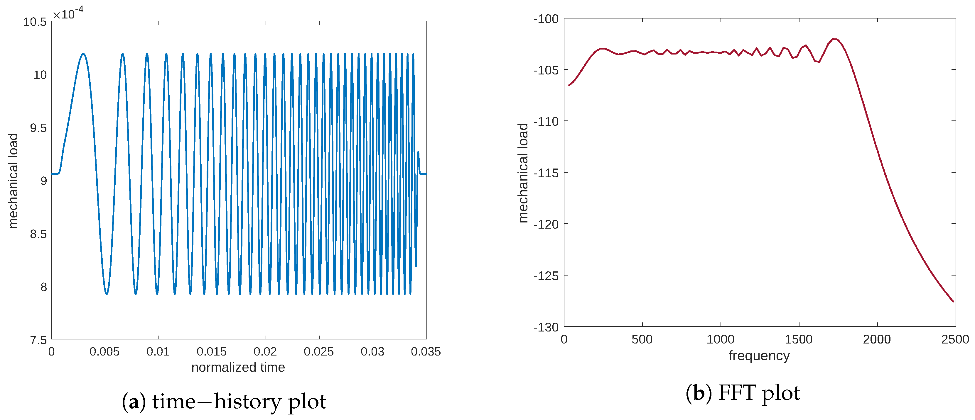
When studying the vibration of a mechanical system, its dynamic behavior is characterized by exciting it through a load with a broad frequency to analyze its response in the same range; here, we proceed to characterize the evolution of the signal associated with the stimulus. Therefore, by utilizing an external load with a wide frequency range, we can identify the dynamic behavior of the tissue by analyzing its response. To this end, we apply a chirp signal to the sample as a mechanical load, as depicted in Figure 2. Figure 2 shows both the time history of the input excitation and its fast Fourier transform (FFT). As can be seen from Figure 2b, the range of frequencies activated, with the same amplitude, is evident. Particularly, the expression of the chirp is as follows:

$$f_{ch}\left(t\right)=F_0+F_{1}sin\left(2\pi f_{i}t+\frac{\pi \Delta f}{T}{t}^2\right)w_T\left(t\right)$$

(25)

where $F_0=9.06\times {10}^{-4}{Y}_{\mathrm{b}}^{\mathrm{Max}}L$ and $F_1=1.13\times {10}^{-4}{Y}_{\mathrm{b}}^{\mathrm{Max}}L$ are the levels of the force per unit line, both static and dynamic, respectively; $f_i=1.0\times {10}^{-4}$ cycles per $t_{ref}$ (c.p.t.) is the initial frequency, $\Delta f=1980$ c.p.t. is the frequency range examined, $T=0.035t_{ref}$ is the time interval of excitation, and $w_T$ is a Tukey tapered cosine window used to simplify the frequency analysis.

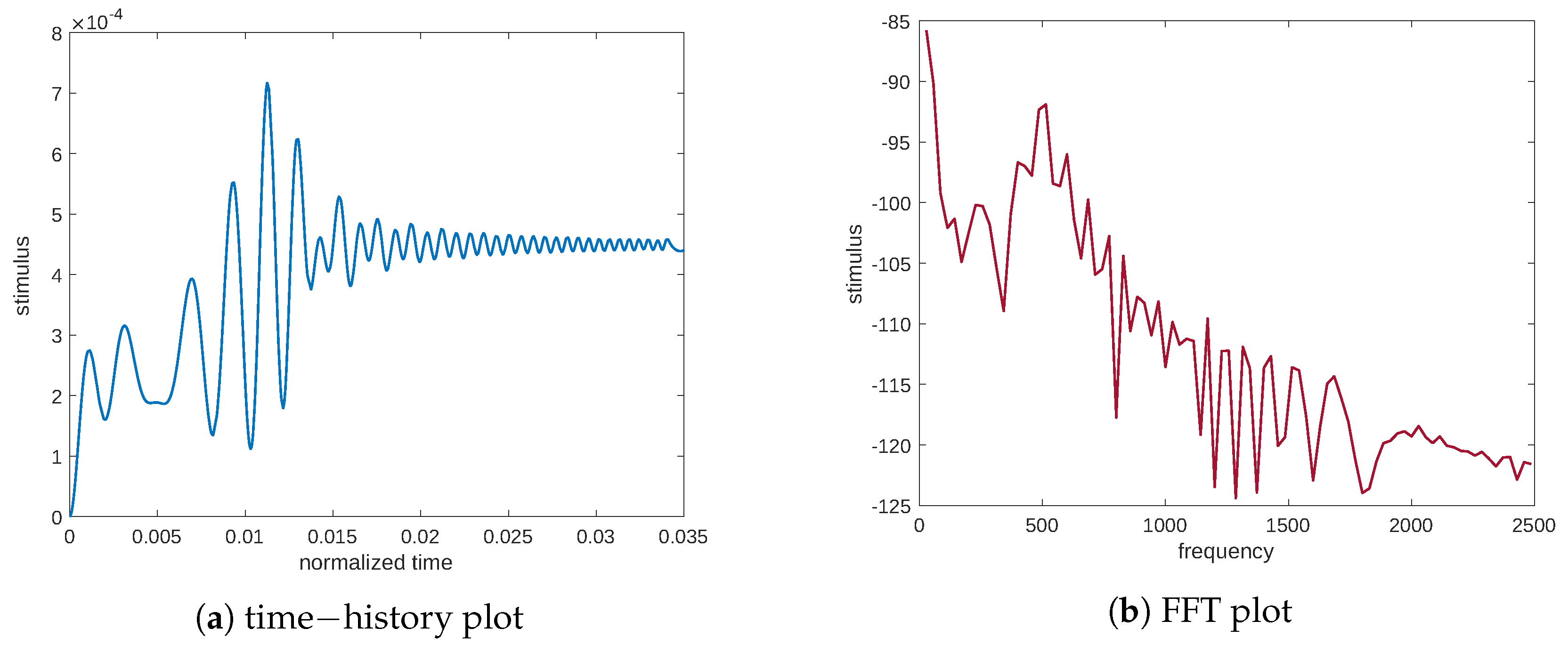
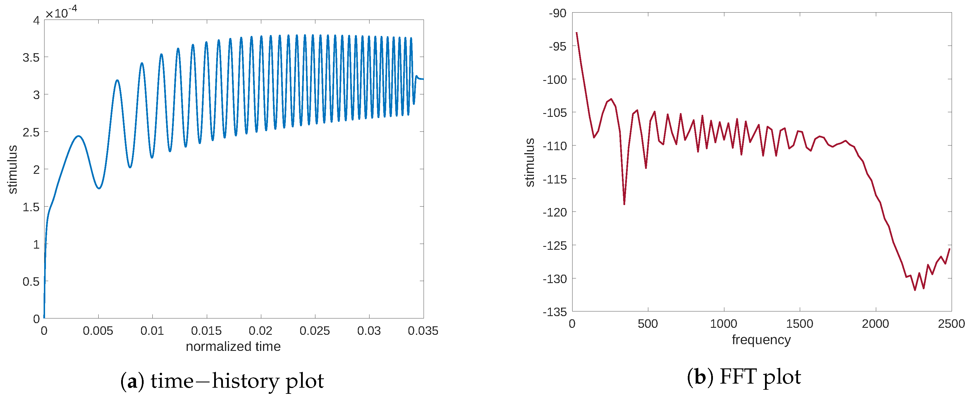
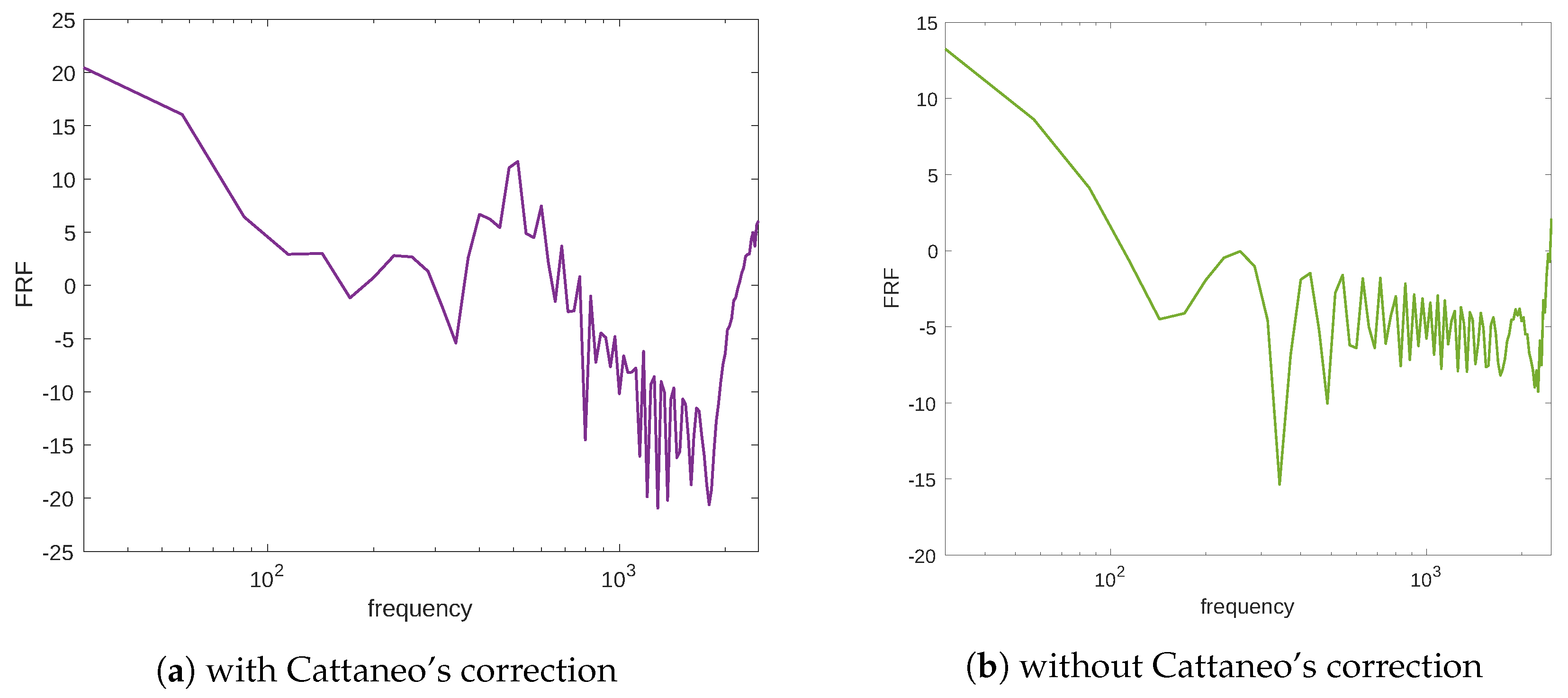
The stimulus produced in response to this load is exhibited in Figure 3. Again, we report both the time and frequency plots of the analyzed signal to decipher the response of the system concerning the stimulus. These plots demonstrate the presence of a natural frequency, $f_{\mathrm{R}}\sim 500$ c.p.t., at which point the system response is the greatest. This frequency could be interpreted as a signal resonance. This behavior is also easier to understand if one considers the frequency response function (FRF) linking the mechanical excitation and the stimulus, that is, the ratio between the FFT amplitude of the signal output and the mechanical input (see Figure 4a). Moreover, Figure 4b illustrates the frequency response function of the stimulus in the case of the diffusion equation without Cattaneo’s correction, i.e., the first term in Equation (3) $\left({\tau }_0\frac{{\partial }^{2}S}{\partial t^2}\right)$. The substantial difference between Figure 4a,b is the resonance peak in the amplitude of the FRF, which is present in Cattaneo’s equation but is absent for the typical diffusion equation (which is a parabolic PDE). 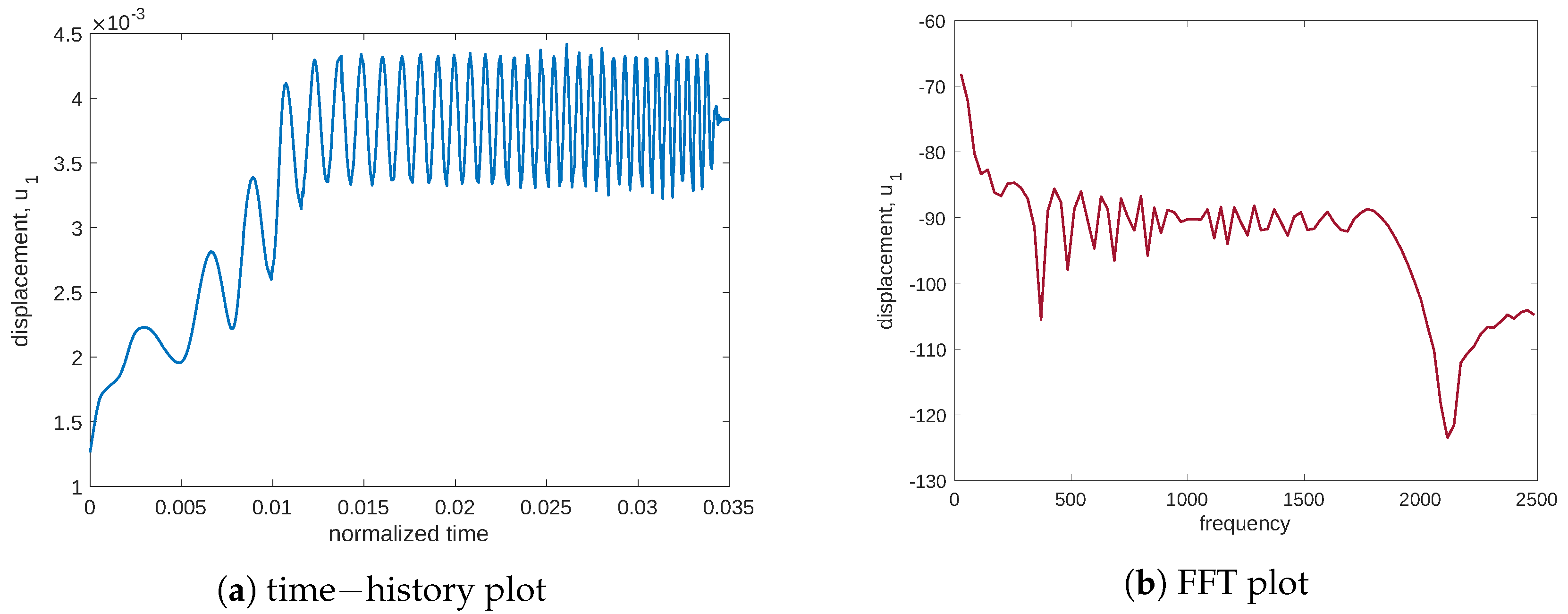Analogous considerations can be made for the resulting stimulus which is evaluated numerically using the diffusion equation without Cattaneo’s correction (see Figure 5 for both plots in time and frequency), where the peak is absent. To fully depict the situation, we also report displacement in the load application (see Figure 6) with a representative point of coordinates $(0.5L,0.25L)$. We note that the initial drift detected in Figure 6a is related to the resorption of the mass that produces a decrease in the elastic modulus. The plots in time and frequency prove that no mechanical resonance is present in the examined range. Therefore, the particular behavior of the stimulus is caused by another source. Indeed, Cattaneo’s equation helps to detect this behavior.

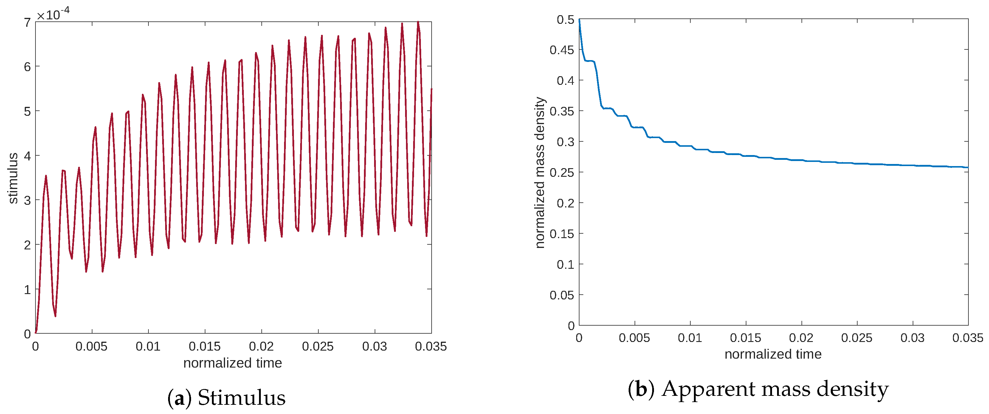
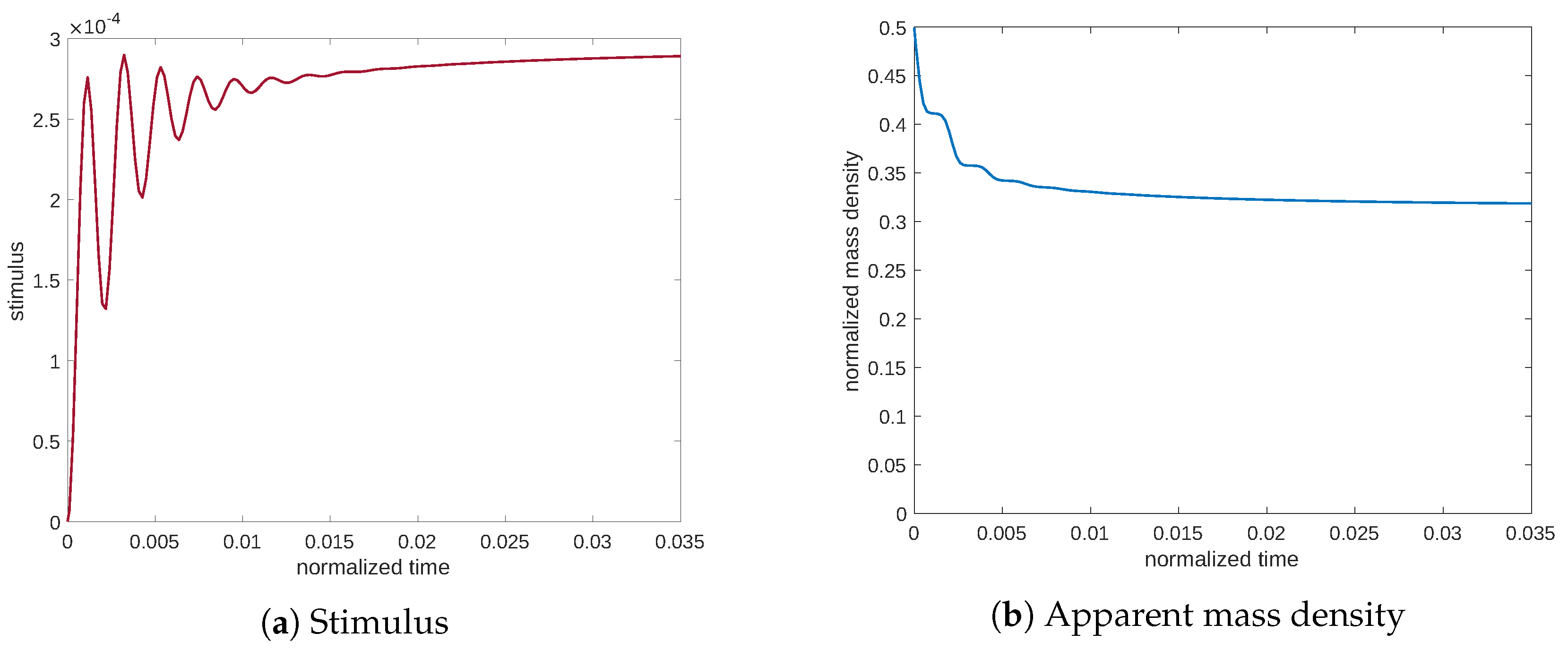
The way that the resonance of the stimulus signal affects the evolution of the bone tissue is illustrated in the three possible scenarios with time-varying loads. We performed the simulations by applying a sinusoidal force with a non-zero average value at the resonance and further from it with a lower (0.35 $f_{\mathrm{R}}$) and a higher (1.4 $f_{\mathrm{R}}$) frequency, of $f_{ex}$, as follows:

$$f_{mn}\left(t\right)=F_0+F_{1}sin\left(2\pi f_{ex}t\right)$$

(26)

in which $F_0=9.06\times {10}^{-4}{Y}_{\mathrm{b}}^{\mathrm{Max}}L$ and $F_1=3.02\times {10}^{-4}{Y}_{\mathrm{b}}^{\mathrm{Max}}L$.

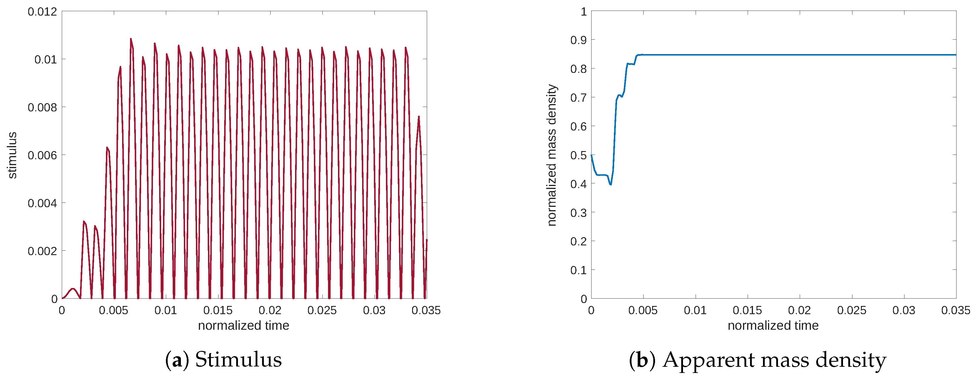
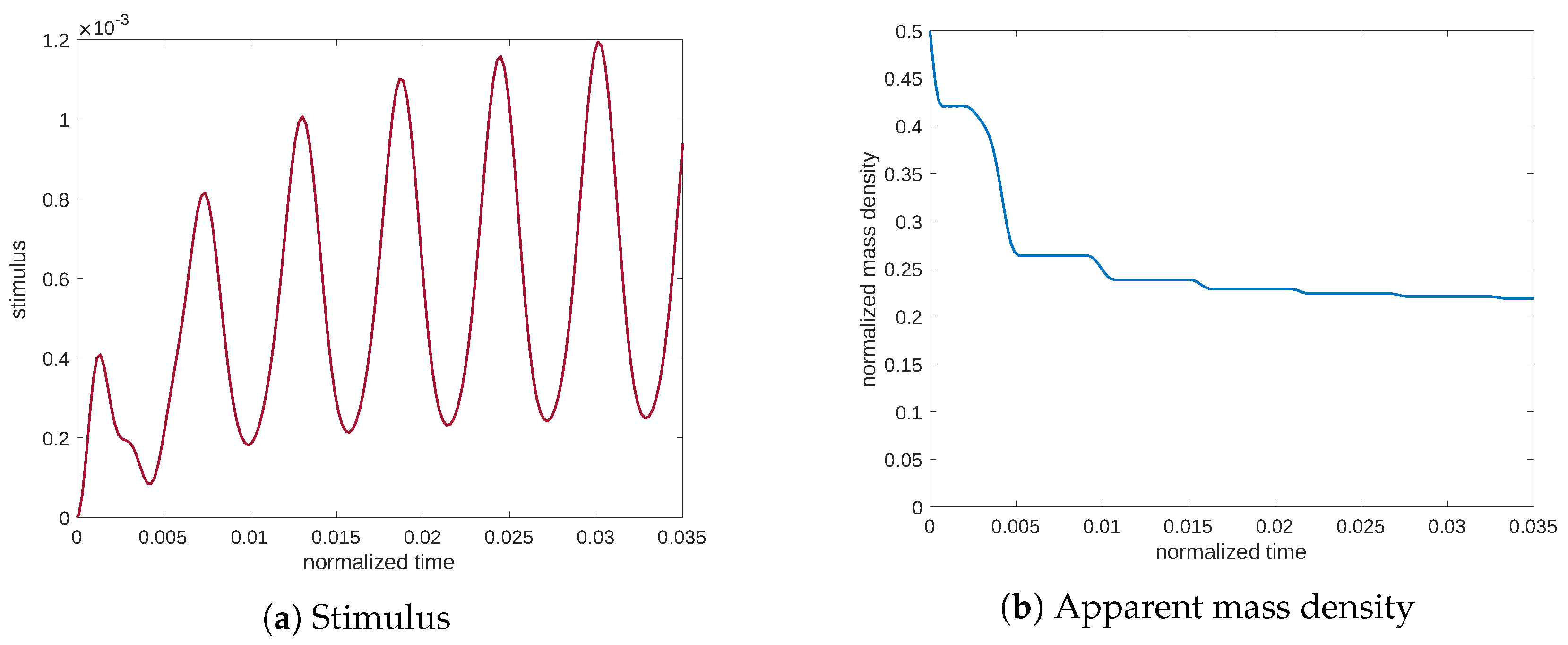
Figure 7 shows the evolution at the resonance of the stimulus and the mass density. The stimulus achieves significantly high values; consequently, the apparent mass density approaches a high value near the minimum of porosity (see Equation (11)). On the contrary, in Figure 8 and Figure 9, related to frequencies of lower and higher than the resonance frequency, we can observe that the stimulus remains lower, after which the mass density undergoes resorption.

Finally, a static case was simulated by considering only the application of a constant force of amplitude $F_0$. Figure 10 displays the evolution of the stimulus and the apparent mass density. Additionally, in this case, the excitation is not sufficiently high to produce new bone; in contrast, the process results in the resorption of old bone.

This behavior, captured by our model based on Cattaneo’s equation, is in accordance with the experiments, where the synthesis seems to be particularly stimulated in correspondence to a resonance frequency value and less influenced by a static load. The diffusion equation alone cannot explain the observed behavior related to the dynamic regime. In the performed numerical simulations, we are thus able to replicate the well-known time-dependence of the bone tissue evolution due to the hyperbolic nature of Cattaneo’s equation and the feedback action occurring in the bone remodeling of the elastic moduli, which couple the mechanical system with the process of signaling transmission. In fact, the mechanical load exciting a piece of bone drives the stimulus and its propagation in the tissue. Since the tissue is finite in size, this propagation can excite an oscillatory mode of the stimulus that resonates at a particular discrete spectrum of frequencies, precisely in the same way as the mechanical modes in a deformable body. Indeed, the equations describing these two phenomena, namely, the oscillation of the stimulus and the mechanical vibrations, are of the same kind.

5. Conclusions

In this paper, we propose a novel formulation for the mechanical stimulus that is able to match the qualitative behavior of the phenomena involved in the remodeling process. The original and important aspect of our model lies in the use of Cattaneo’s equation to mimic the diffusion and propagation nature of the mechanically driven biological stimulus that controls the entire process. The hyperbolic character of the equation facilitates the natural oscillatory modes for the stimulus that can resonate in some sense with the external mechanical excitations and amplify the adaptive response of bone tissue selectively at a discrete spectrum of natural frequencies.

Numerical simulations with the newly proposed model were constructed. Clearly, they show that this kind of formulation is able to describe some of the crucial aspects of bone remodeling, including, among other things, the influence of dynamic loads. The evolution of a 2D bone sample under a dynamic tensile test was evaluated; under some cases of cyclic loads, the responses were found to be completely distinct, depending solely on the excitation frequency. New bone tissue growth is promoted only for external mechanical excitations at a given frequency. These preliminary results are encouraging but require more investigations that will be carried out in future works.

Finally, as observed in the Introduction, the study of bone remodeling could include also intercellular and intracellular signaling, which will be the subject of future work, based on the well-known biochemical Michaelis–Menten kinetics (see, e.g., [75,76]).