
Supervised Machine Learning–Based Detection of Concrete Efflorescence

Abstract
:1. Introduction
2. Literature Review
3. Research Methods and Materials
3.1. Machine Learning Classifiers
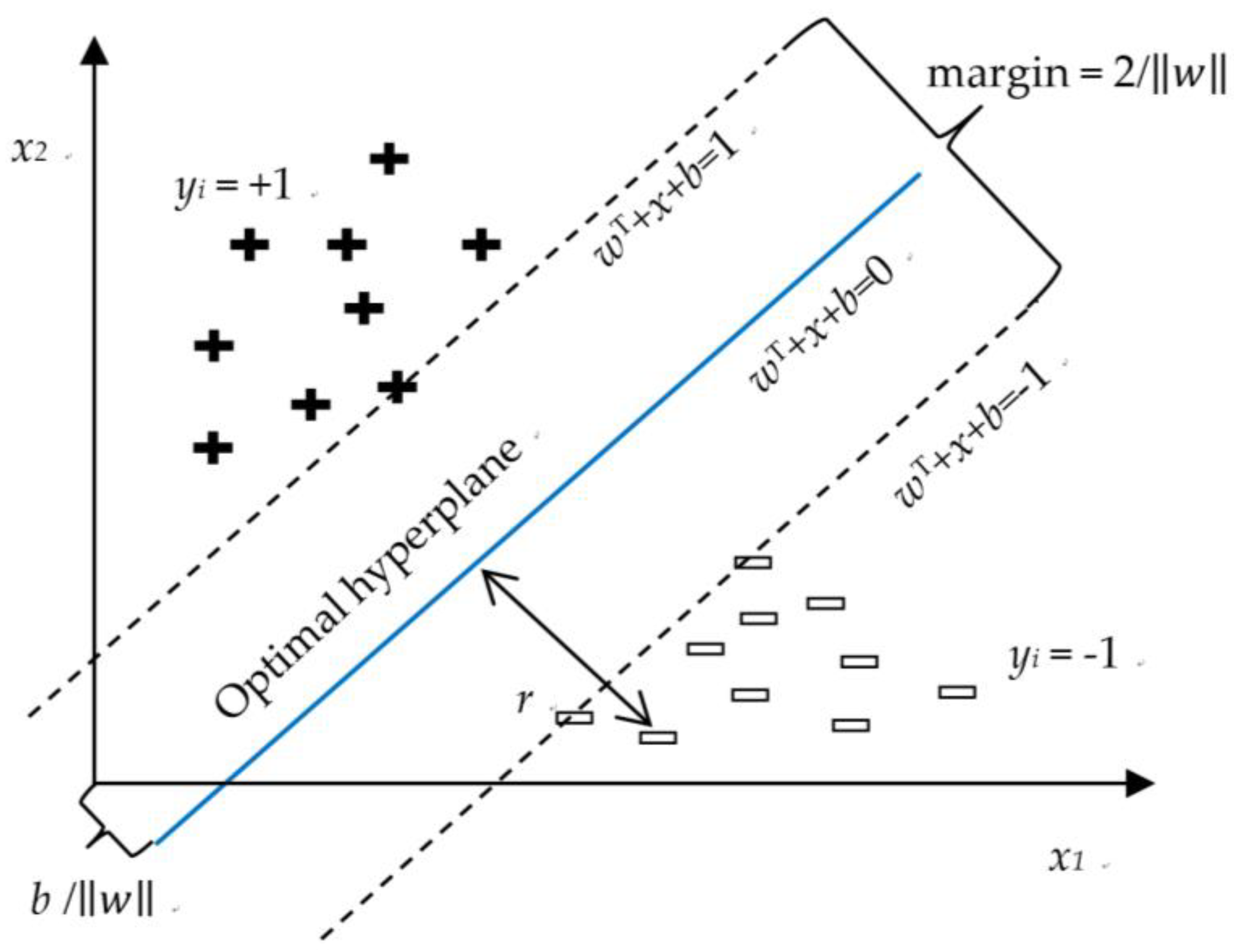
3.1.1. Support Vector Machine (SVM)
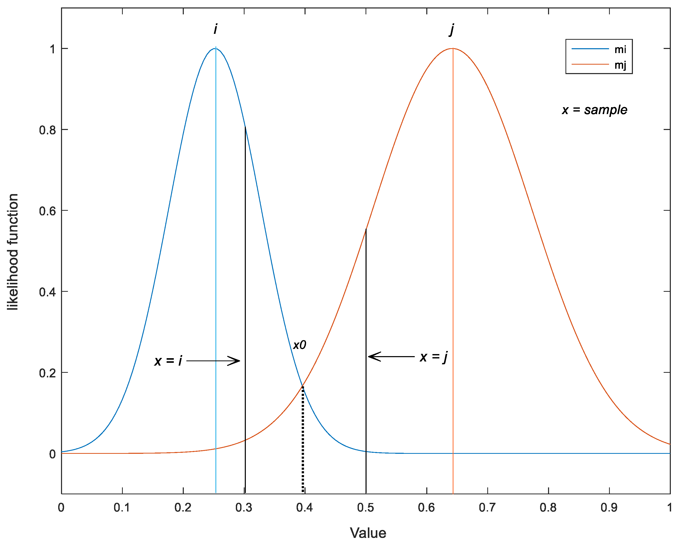
3.1.2. Maximum Likelihood (ML)
3.1.3. Random Forest (RF)
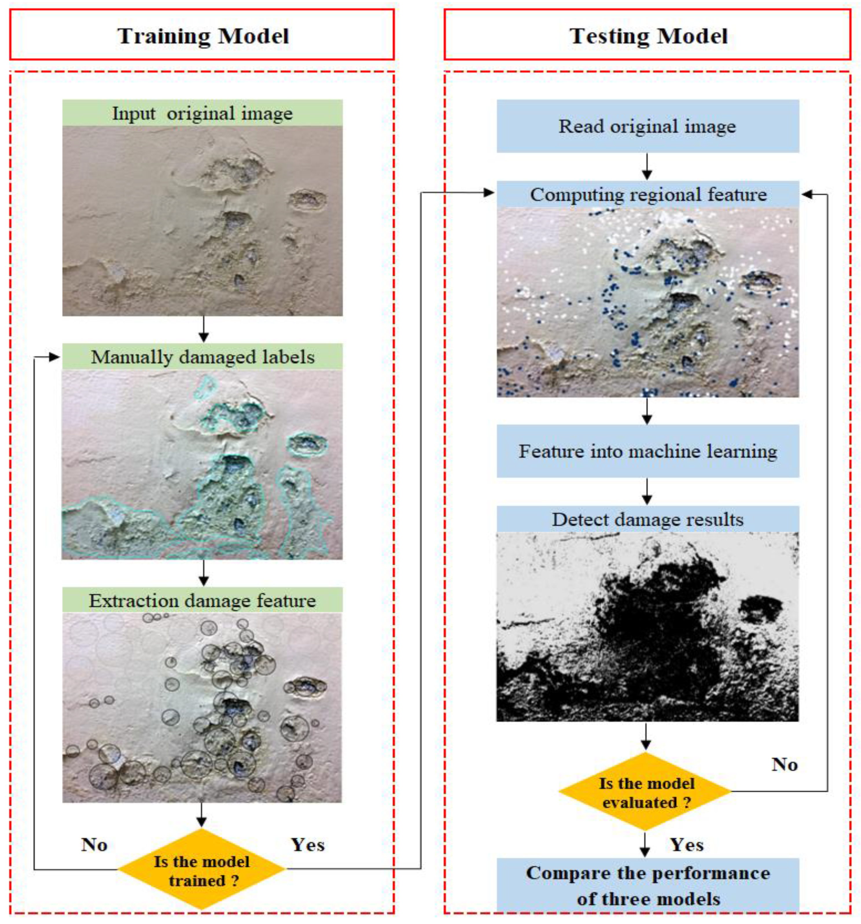
3.2. Material and Image Processing
4. Model Evaluation Indicators
4.1. Accuracy
4.2. Precision and Recall
4.3. F1
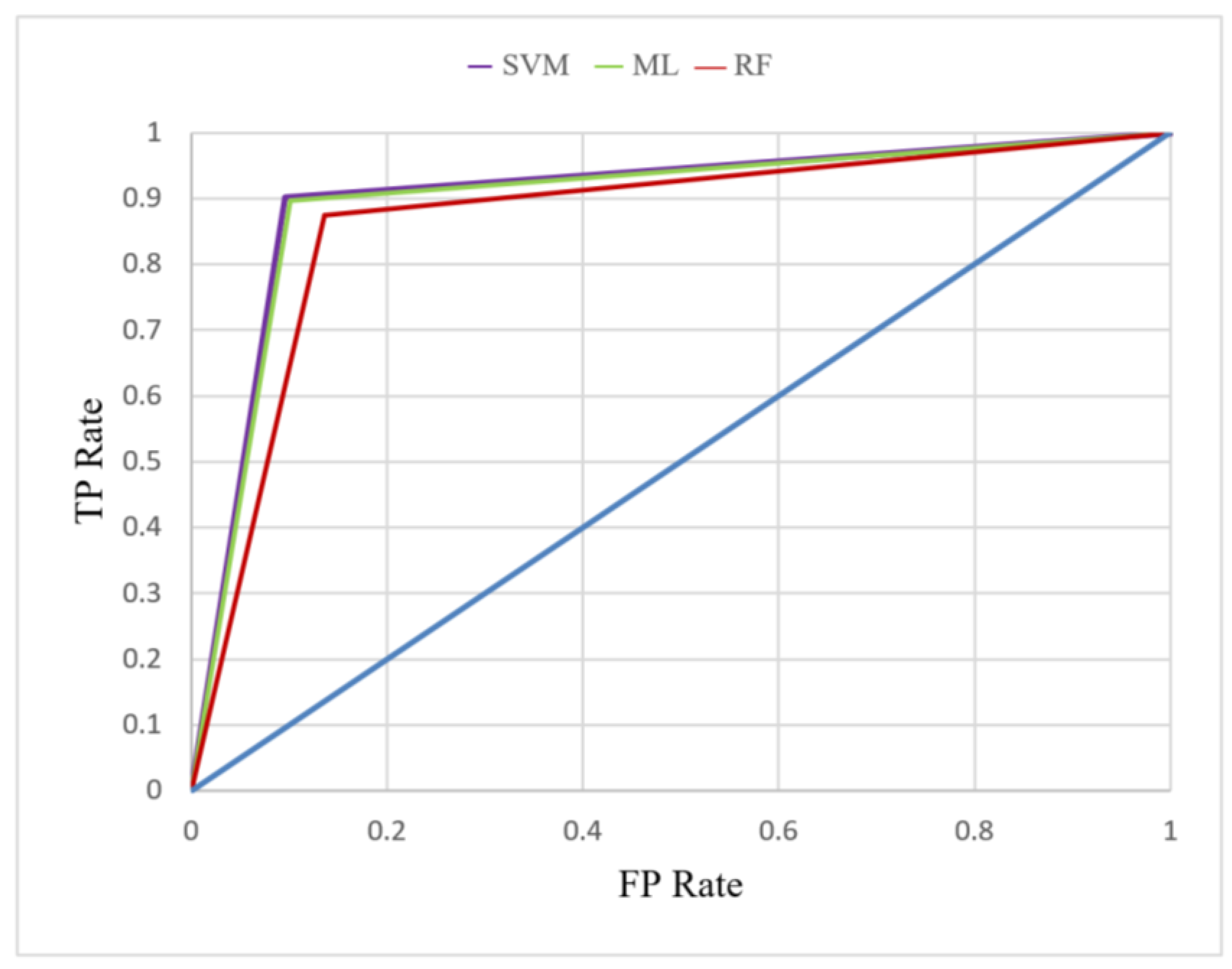
4.4. ROC, AUC, and Gini Coefficient
4.5. Kappa
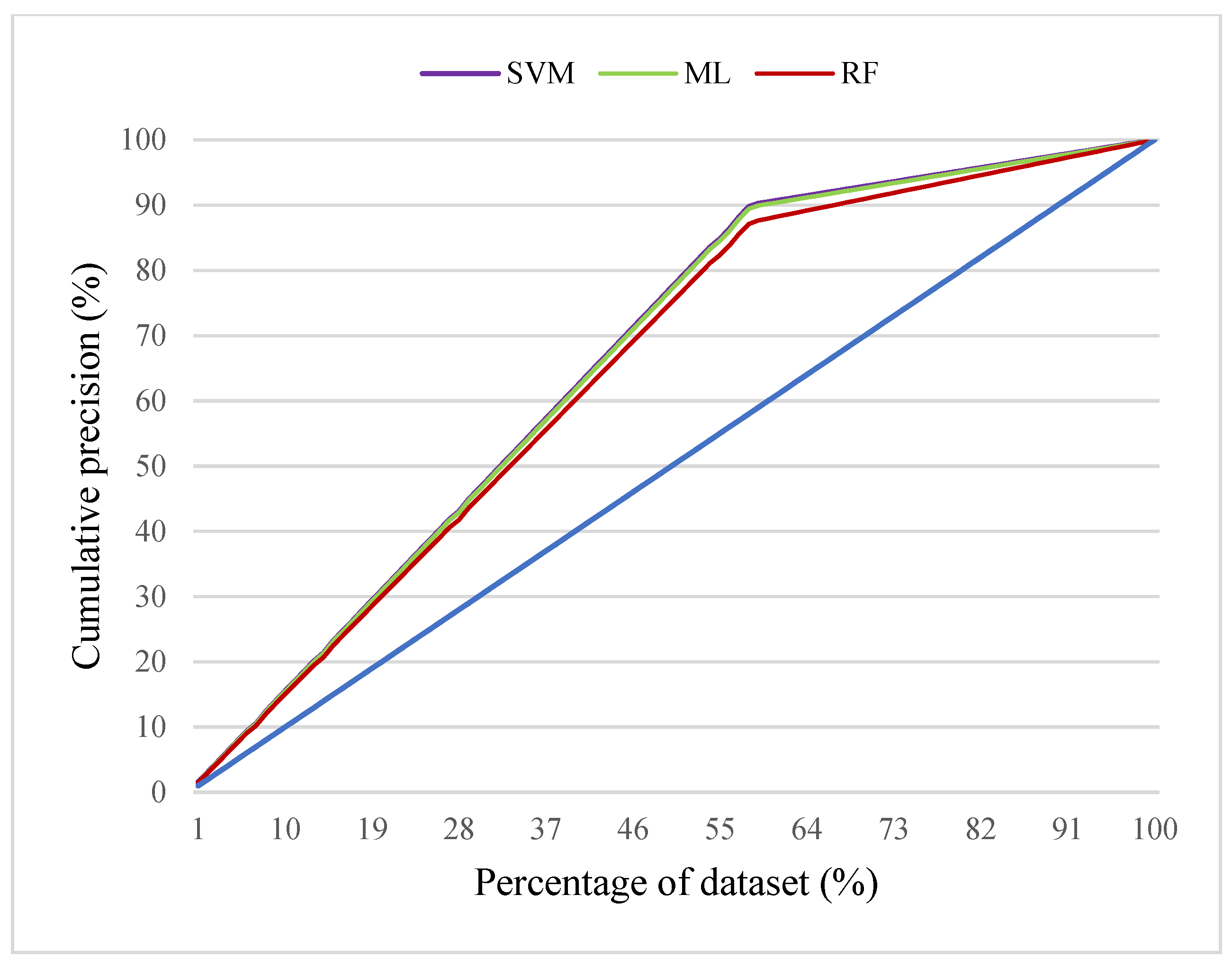
4.6. Gain Chart
5. Results and Discussion
5.1. Evaluation of Classification Models
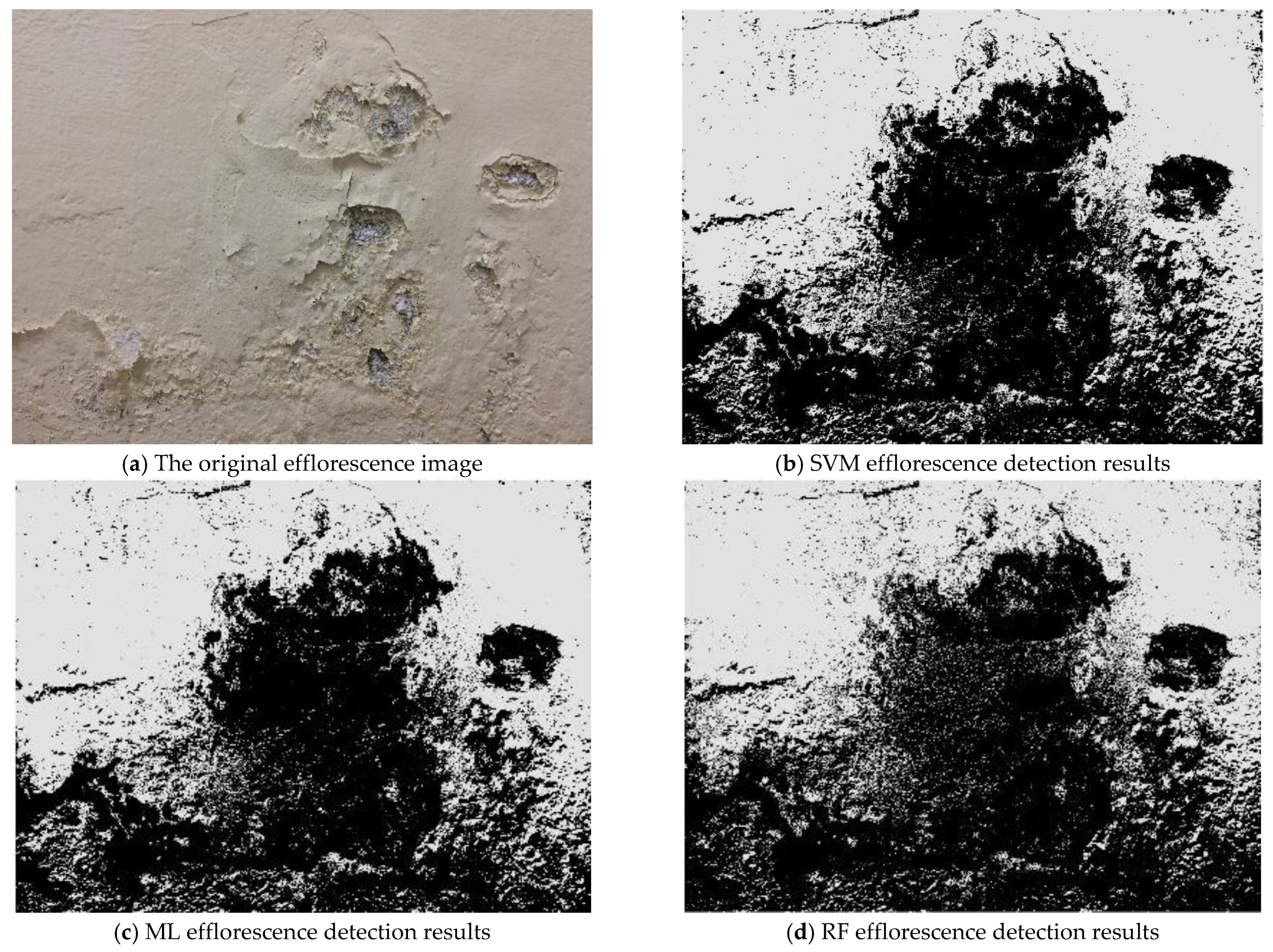
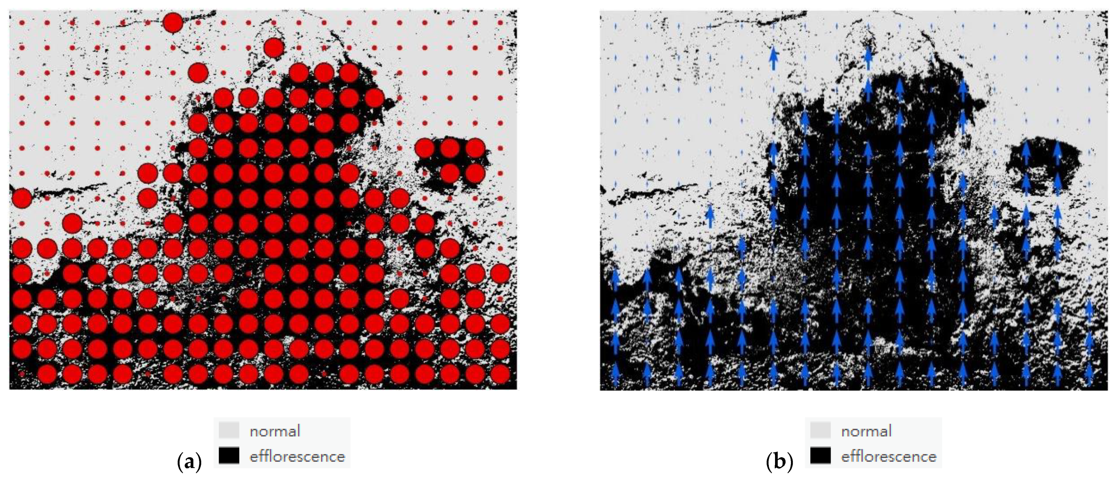
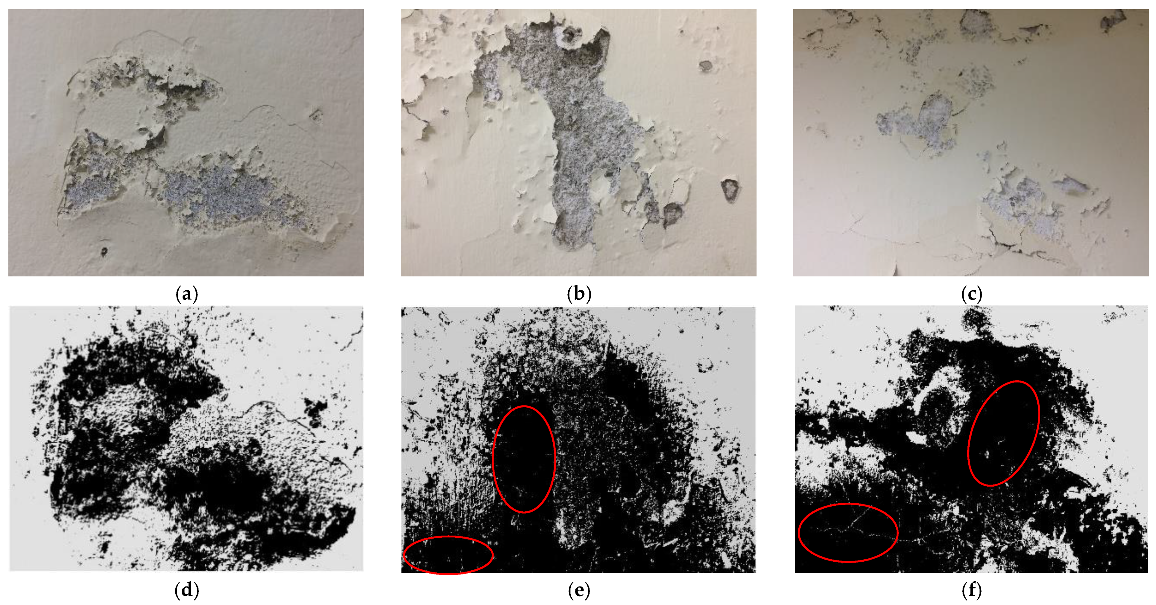
5.2. Efflorescence Detection Results
6. Conclusions
Author Contributions
Funding
Data Availability Statement
Conflicts of Interest
References
- Hüthwohl, P.; Brilakis, I.; Borrmann, A.; Sacks, R. Integrating RC bridge defect information into BIM models. J. Comput. Civ. Eng. 2018, 32. [Google Scholar] [CrossRef]
- ASTM C1400-11; Standard Guide for Reduction of Efflorescence Potential in New Masonry Walls. ASTM International: West Conshohocken, PA, USA, 2017.
- ASTM C67-02c; Standard Test Methods for Sampling and Testing Brick and Structural Clay Tile. ASTM International: West Conshohocken, PA, USA, 2002.
- Ada, M.; Sevim, B.; Yüzer, N.; Ayvaz, Y. Assessment of damages on a RC building after a big fire. Adv. Concr. Constr. 2018, 6, 177–197. [Google Scholar]
- Phares, B.M.; Washer, G.A.; Rolander, D.D.; Graybeal, B.A.; Moore, M. Routine highway bridge inspection condition documentation accuracy and reliability. J. Bridg. Eng. 2014, 9, 403–413. [Google Scholar] [CrossRef]
- Bianchini, A.; Bandini, P.; Smith, D.W. Interrater reliability of manual pavement distress evaluations. J. Transp. Eng. 2010, 136, 165–172. [Google Scholar] [CrossRef]
- Zhu, Z.; Brilakis, I. Parameter optimization for automated concrete detection in image data. Autom. Constr. 2010, 19, 944–953. [Google Scholar] [CrossRef]
- Cha, Y.J.; Chen, J.G.; Büyüköztürk, O. Output-only computer vision based damage detection using phase-based optical flow and unscented Kalman filters. Eng. Struct. 2017, 132, 300–313. [Google Scholar] [CrossRef]
- Chen, J.G.; Wadhwa, N.; Cha, Y.J.; Durand, F.; Freeman, W.T.; Buyukozturk, O. Modal identification of simple structures with high-speed video using motion magnification. J. Sound. Vib. 2015, 345, 58–71. [Google Scholar] [CrossRef]
- Cha, Y.J.; Choi, W.; Büyüköztürk, O. Deep learning-based crack damage detection using convolutional neural networks. Comput. Civ. Infrastruct. Eng. 2017, 32, 361–378. [Google Scholar] [CrossRef]
- Zhang, Y.; Yuen, K.V. Review of artificial intelligence-based bridge damage detection. Adv. Mech. Eng. 2022, 14, 16878132221122770. [Google Scholar] [CrossRef]
- Yoo, H.S.; Kim, Y.S. Development of a crack recognition algorithm from non-routed pavement images using artificial neural network and binary logistic regression. KSCE J. Civ. Eng. 2016, 20, 1151–1162. [Google Scholar] [CrossRef]
- Abdel-Qader, I.; Pashaie-Rad, S.; Abudayyeh, O.; Yehia, S. PCA-based algorithm for unsupervised bridge crack detection. Adv. Eng. Softw. 2006, 37, 771–778. [Google Scholar] [CrossRef]
- Lattanzi, D.; Miller, G.R. Robust automated concrete damage detection algorithms for field applications. J. Comput. Civ. Eng. 2014, 28, 253–262. [Google Scholar] [CrossRef]
- Choubey, R.K.; Kumar, S.; Rao, M.C. Effect of shear-span/depth ratio on cohesive crack and double-K fracture parameters of concrete. Adv. Concr. Constr. 2014, 2, 229–247. [Google Scholar] [CrossRef]
- Haeri, H.; Sarfarazi, V.; Zhu, Z.; Nejati, H.R. Numerical simulations of fracture shear test in anisotropy rocks with bedding layers. Adv. Concr. Constr. 2019, 7, 241–247. [Google Scholar]
- Ayinde, O.O.; Zuo, X.B.; Yin, G.J. Numerical analysis of concrete degradation due to chloride-induced. Adv. Concr. Constr. 2019, 7, 203–210. [Google Scholar]
- Zhang, B.; Cullen, M.; Kilpatrick, T. Spalling of heated high performance concrete due to thermal and hygric gradients. Adv. Concr. Constr. 2016, 4, 1–14. [Google Scholar] [CrossRef]
- Adhikari, R.S.; Moselhi, O.; Bagchi, A.; Rahmatian, A. Tracking of defects in reinforced concrete bridges using digital images. J. Comput. Civ. Eng. 2016, 30, 04016004. [Google Scholar] [CrossRef]
- Patange, A.D.; Jegadeeshwaran, R. A machine learning approach for vibration-based multipoint tool insert health prediction on vertical machining centre (VMC). Measurement 2021, 173, 108649. [Google Scholar] [CrossRef]
- German, S.; Brilakis, I.; Desroches, R. Rapid entropy-based detection and properties measurement of concrete spalling with machine vision for post-earthquake safety assessments. Adv. Eng. Inform. 2012, 26, 846–858. [Google Scholar] [CrossRef]
- Brilakis, I.; Fathi, H.; Rashidi, A. Progressive 3D reconstruction of infrastructure with videogrammetry. Autom. Constr. 2011, 20, 884–895. [Google Scholar] [CrossRef]
- Rashidi, A.; Sigari, M.H.; Maghiar, M.; Citrin, D. An analogy between various machine-learning technologys for detecting construction materials in digital images. KSCE J. Civ. Eng. 2016, 20, 1178–1188. [Google Scholar] [CrossRef]
- Radopoulou, S.C.; Brilakis, I. Automated detection of multiple pavement defects. J. Comput. Civ. Eng. 2017, 31. [Google Scholar] [CrossRef] [Green Version]
- Zhou, S.; Chen, Y.; Zhang, D.; Xie, J.; Zhou, Y. Classification of surface defects on steel sheet using convolutional neural networks. Mater. Tehnol. 2017, 51, 123–131. [Google Scholar] [CrossRef]
- Halfawy, M.R.; Hengmeechai, J. Automated defect detection in sewer closed circuit television images using histograms of oriented gradients and support vector machine. Autom. Constr. 2014, 38, 1–13. [Google Scholar] [CrossRef]
- Mountrakis, G.; Im, J.; Ogole, C. Support vector machines in remote sensing: A review. ISPRS J. Photogramm. Remote Sens. 2011, 66, 247–259. [Google Scholar] [CrossRef]
- Pal, M.; Foody, G.M. Feature selection for classification of hyperspectral data by SVM. IEEE Trans. Geosci. Remote Sens. 2010, 48, 2297–2307. [Google Scholar] [CrossRef] [Green Version]
- Ali, S.; Smith, K.A. On learning algorithm selection for classification. Appl. Soft Comput. J. 2006, 6, 119–138. [Google Scholar] [CrossRef]
- Kim, C.; Son, H.; Kim, C. Automated color model-based concrete detection in construction-site images by using machine learning algorithms. J. Comput. Civ. Eng. 2012, 26, 421–433. [Google Scholar]
- Chen, P.H.; Shen, H.K.; Lei, C.Y.; Chang, L.M. Support-vector-machine-based method for automated steel bridge rust assessment. Autom. Constr. 2012, 23, 9–19. [Google Scholar] [CrossRef]
- Lu, D.; Mausel, P.; Batistella, M.; Moran, E. Comparison of land-cover classification methods in the Brazilian Amazon basin. Photogramm. Eng. Remote Sens. 2004, 6, 723–731. [Google Scholar] [CrossRef] [Green Version]
- Guo, L.; Chehata, N.; Mallet, C.; Boukir, S. Relevance of airborne lidar and multispectral image data for urban scene classification using Random Forests. ISPRS J. Photogramm. Remote Sens. 2011, 66, 56–66. [Google Scholar] [CrossRef]
- Alipour, M.; Harris, D.K.; Barnes, L.E.; Ozbulut, O.E.; Carroll, J. Load-capacity rating of bridge populations through machine learning: Application of decision trees and random forests. J. Bridg. Eng. 2017, 22, 04017076. [Google Scholar] [CrossRef]
- Assouline, D.; Mohajeri, N.; Scartezzini, J.L. Building rooftop classification using random forests for large-scale PV deployment. In Proceedings of the Earth Resources and Environmental Remote Sensing/GIS Applications VIII, Warsaw, Poland, 5 October 2017; pp. 47–58. [Google Scholar]
- Harvey, R.R.; McBean, E.A. Predicting the structural condition of individual sanitary sewer pipes with random forests. Can. J. Civ. Eng. 2014, 41, 294–303. [Google Scholar] [CrossRef]
- Kim, C.; Son, H.; Hwang, N.; Kim, C.; Kim, C. Rapid and automated determination of rusted surface areas of a steel bridge for robotic maintenance systems. Autom. Constr. 2014, 42, 13–24. [Google Scholar]
- Yeh, I.C. Quantity estimating of building with logarithm-neuron networks. J. Const. Eng. Manag. 1998, 124, 374–380. [Google Scholar] [CrossRef]
- Tam, C.M.; Tong, K.L.; Lau, T.C.; Chan, K.K. Diagnosis of prestressed concrete pile defects using probabilistic neural networks. Eng. Struct. 2004, 26, 1155–1162. [Google Scholar] [CrossRef]
- Ruiz, C.C.; Caballero, J.L.; Martinez, J.H.; Aperador, W.A. Algorithms to measure carbonation depth in concrete structures sprayed with a phenolphthalein solution. Adv. Concr. Constr. 2020, 9, 257–265. [Google Scholar]
- Mathavan, S.; Rahman, M.; Kamal, K. Use of a self-organizing map for crack detection in highly textured pavement images. J. Infrastruct. Syst. 2015, 21, 04014052. [Google Scholar] [CrossRef]
- Ngwangwa, H.M.; Heyns, P.S.; Labuschagne, F.J.J.; Kululanga, G.K. Reconstruction of road defects and road roughness classification using vehicle responses with artificial neural networks simulation. J. Terramech. 2010, 47, 97–111. [Google Scholar] [CrossRef] [Green Version]
- Wu, L.; Mokhtari, S.; Nazef, A.; Nam, B.; Yun, H.B. Improvement of crack-detection accuracy using a novel crack defragmentation technology in image-based road assessment. J. Comput. Civ. Eng. 2019, 30, 04014118. [Google Scholar] [CrossRef]
- Bajaj, N.S.; Patange, A.D.; Jegadeeshwaran, R.; Kulkarni, K.A.; Ghatpande, R.S.; Kapadnis, A.M. A bayesian optimized discriminant analysis model for condition monitoring of face milling cutter using vibration datasets. J. Nondest. Eval. Diagn. Progn. Eng. Syst. 2022, 5, 021002. [Google Scholar] [CrossRef]
- Jatakar, K.H.; Mulgund, G.; Patange, A.D.; Deshmukh, B.B.; Rambhada, K.S. Multi-Point face milling tool condition monitoring through vibration spectrogram and LSTM-Autoencoder. Int. J. Perform. Eng. 2022, 18, 570–579. [Google Scholar] [CrossRef]
- Patil, S.S.; Pardeshi, S.S.; Pradhan, N.; Patange, A.D. Cutting tool condition monitoring using a deep learning-based artificial neural network. Int. J. Perform. Eng. 2022, 18, 37–46. [Google Scholar]
- Koch, C.; Georgieva, K.; Kasireddy, V.; Akinci, B.; Fieguth, P. A review on computer vision based defect detection and condition assessment of concrete and asphalt civil infrastructure. Adv. Eng. Inform. 2015, 29, 196–210. [Google Scholar] [CrossRef] [Green Version]
- Meijer, D.; Scholten, L.; Clemens, F.; Knobbe, A. A defect classification methodology for sewer image sets with convolutional neural networks. Autom. Constr. 2019, 104, 281–298. [Google Scholar] [CrossRef]
- Gonzalez, R.C.; Woods, R.E. Digital Image Processing; Prentice Hall: Hoboken, NJ, USA, 2008. [Google Scholar]
- Bengio, Y.; Courville, A.; Vincent, P. Representation learning: A review and new perspectives. IEEE Trans. Pattern Anal. Mach. Intell. 2013, 35, 1798–1828. [Google Scholar] [CrossRef] [Green Version]
- Vapnik, V.N. The Nature of Statistical Learning Theory; Springer: New York, NY, USA, 1995. [Google Scholar]
- Richards, J. Remote Sensing Digital Image Analysis; Springer: Berlin, Germany, 1999. [Google Scholar]
- Breiman, L. Random forests. Mach. Learn. 2001, 45, 5–32. [Google Scholar] [CrossRef]
- Castagno, J.; Atkins, E. Roof shape classification from LiDAR and satellite image data fusion using supervised learning. Sensors 2018, 18, 3960. [Google Scholar] [CrossRef] [Green Version]
- Meyer, H.; Reudenbach, C.; Hengl, T.; Katurji, M.; Nauss, T. Improving performance of spatio-temporal machine learning models using forward feature selection and target-oriented validation. Environ. Model Softw. 2018, 101, 1–9. [Google Scholar] [CrossRef]
- Xiao, Y.; Feng, C.; Taguchi, Y.; Kamat, V.R. User-guided dimensional analysis of indoor building environments from single frames of RGB-D sensors. J. Comput. Civ. Eng. 2017, 31, 04017006. [Google Scholar] [CrossRef] [Green Version]
- Dawood, T.; Zhu, Z.; Zayed, T. Machine vision-based model for spalling detection and quantification in subway networks. Autom. Constr. 2017, 81, 149–160. [Google Scholar] [CrossRef]
- German, S.; Jeon, J.S.; Zhu, Z.; Bearman, C.; Brilakis, I.; DesRoches, R.; Lowes, L. Machine vision-enhanced postearthquake inspection. J. Comput. Civ. Eng. 2013, 27, 622–634. [Google Scholar] [CrossRef]
- Halfawy, M.R.; Hengmeechai, J. Integrated vision-based system for automated defect detection in sewer closed circuit television inspection videos. J. Comput. Civ. Eng. 2015, 29, 04014024. [Google Scholar] [CrossRef]
- Koch, C.; Jog, G.M.; Brilakis, I. Automated pothole distress assessment using asphalt pavement video data. J. Comput. Civ. Eng. 2013, 27, 370–378. [Google Scholar] [CrossRef]
- Hüthwohl, P.; Lu, R.; Brilakis, I. Multi-classifier for reinforced concrete bridge defects. Autom. Constr. 2019, 105, 102824. [Google Scholar] [CrossRef]
- Hüthwohl, P.; Brilakis, I. Detecting healthy concrete surfaces. Adv. Eng. Inform. 2018, 37, 150–162. [Google Scholar] [CrossRef]
- Kohavi, R.; Provost, F. Glossary of terms. Mach. Learn. 1998, 30, 271–274. [Google Scholar]
- Van Rijsbergen, C.J. Information Retrieval; Butterworths: London, UK, 1979. [Google Scholar]
- Fawcett, T. An introduction to ROC analysis. Pattern Recogn. Lett. 2006, 27, 861–874. [Google Scholar] [CrossRef]
- Cohen, J. A coefficient of agreement for nominal scales. Educ. Psychol. Meas. 1960, 20, 37–46. [Google Scholar] [CrossRef]
- Ben-David, A. Comparison of classification accuracy using Cohen’s weighted Kappa. Expert. Syst. Appl. 2008, 34, 825–832. [Google Scholar] [CrossRef]
- Foody, G.M. Thematic map comparison: Evaluating the statistical significance of differences in classification accuracy. Photogramm. Eng. Remote Sens. 2004, 5, 627–633. [Google Scholar] [CrossRef]
- Smits, P.C.; Dellepiane, S.G.; Schowengerdt, R.A. Quality assessment of image classification algorithms for land-cover mapping: A review and a proposal for a cost-based approach. Int. J. Remote Sens. 1999, 20, 1461–1486. [Google Scholar] [CrossRef]
- Fung, T.; Ledrew, E. The determination of optimal threshold levels for change detection using various accuracy indices. Photogramm. Eng. Remote Sens. 1988, 54, 1449–1454. [Google Scholar]
- Vetrivel, A.; Gerke, M.; Kerle, N.; Vosselman, G. Identification of structurally damaged areas in airborne oblique images using a Visual-Bag-of-Words approach. Remote Sens. 2016, 8, 231. [Google Scholar] [CrossRef] [Green Version]
- Kim, D.; Kim, D.H.; Chang, S.; Lee, J.J.; Lee, D.H. Stability number prediction for breakwater armor blocks using support vector regression. KSCE J. Civ. Eng. 2011, 15, 225–230. [Google Scholar] [CrossRef]
- Powers, D.M.W. Evaluation: From precision, recall and F-measure to ROC, informedness, markedness & correlation. J. Mach. Learn. Technol. 2011, 2, 37–63. [Google Scholar]
- Gui, G.; Pan, H.; Lin, Z.; Li, Y.; Yuan, Z. Data-driven support vector machine with optimization techniques for structural health monitoring and damage detection. KSCE J. Civ. Eng. 2017, 21, 523–534. [Google Scholar] [CrossRef]
- Kakumanu, P.; Makrogiannis, S.; Bourbakis, N. A survey of skin-color modeling and detection methods. Pattern Recognit. 2007, 40, 1106–1122. [Google Scholar] [CrossRef]
- Li, S.; Zhao, X.; Zhou, G. Automatic pixel-level multiple damage detection of concrete structure using fully convolutional network. Comput. Civ. Infrastruct. Eng. 2019, 34, 616–634. [Google Scholar] [CrossRef]
- Crespo, C.; Armesto, J.; González-Aguilera, D.; Arias, P. Damage detection on historical buildings using unsupervised classification techniques. Int. Arch. Photogramm. Remote Sens. Spat. Inf. Sci. 2010, 38, 184–188. [Google Scholar]
- Bouzan, G.B.; Fazzioni, P.F.; Faisca, R.G.; Soares, C.A. Building facade inspection: A system based on automated data acquisition, machine learning, and deep learning image classification methods. ARPN J. Eng. Appl. Sci. 2021, 16, 1516. [Google Scholar]


| Actual | Classification Results (Predicated) | PA (%) | OE (%) | |
|---|---|---|---|---|
| A | B | |||
| A | True Positive (TP) | False Negative (FN) | TP/(TP + FN) (Sensitivity) | FN/(TP + FN) |
| B | False Positive (FP) | True Negative (TN) | TN/(FP +TN) (Specificity) | FP/(FP +TN) |
| UA (%) | TP/(TP + FP) (Precision) | TN/(FN + TN) | AUC = Mean PA | Accuracy = (TP + TN)/(TP + TN + FP + FN) |
| Number | Indicator | Formula |
|---|---|---|
| (a) | Accuracy | |
| (b) | Precision (P) | |
| (c) | Recall (R) | |
| (d) | F1 | |
| (e) | ROC | X-axis: FP Ratio (1-Specificity); Y-axis: TP Ratio (Sensitivity) |
| (f) | AUC | |
| (g) | Gini coefficient | 2 × AUC − 1 |
| (h) | Kappa | |
| (i) | Gain | X-axis: Percentage of dataset; Y-axis: Cumulative precision |
| Truth | Predicated | PA (%) | OE (%) | |
|---|---|---|---|---|
| Efflorescence | Normal | |||
| efflorescence | 272 | 30 | 90.1 | 9.9 |
| normal | 19 | 179 | 90.4 | 9.6 |
| UA (%) | 93.4 | 85.6 | Accuracy = 90.2% | |
| CE (%) | 6.6 | 14.4 | n = 500 | |
| Truth | Predicated | PA (%) | OE (%) | |
|---|---|---|---|---|
| Efflorescence | Normal | |||
| efflorescence | 271 | 31 | 89.7 | 10.3 |
| normal | 20 | 178 | 89.9 | 10.1 |
| UA (%) | 93.1 | 85.2 | Accuracy = 89.8% | |
| CE (%) | 6.9 | 14.8 | n = 500 | |
| Truth | Predicated | PA (%) | OE (%) | |
|---|---|---|---|---|
| Efflorescence | Normal | |||
| efflorescence | 264 | 38 | 87.4 | 12.6 |
| normal | 27 | 171 | 86.4 | 13.6 |
| UA (%) | 90.7 | 81.8 | Accuracy = 87.0% | |
| CE (%) | 9.3 | 18.2 | n = 500 | |
| Accuracy | F1 | AUC | Gini | Kappa | Gain | |
|---|---|---|---|---|---|---|
| SVM | 0.902 | 0.880 | 0.902 | 0.805 | 0.797 | 0.774 |
| ML | 0.898 | 0.874 | 0.898 | 0.796 | 0.789 | 0.771 |
| RF | 0.870 | 0.839 | 0.869 | 0.738 | 0.731 | 0.751 |
Publisher’s Note: MDPI stays neutral with regard to jurisdictional claims in published maps and institutional affiliations. |
© 2022 by the authors. Licensee MDPI, Basel, Switzerland. This article is an open access article distributed under the terms and conditions of the Creative Commons Attribution (CC BY) license (https://creativecommons.org/licenses/by/4.0/).
Share and Cite
Fan, C.-L.; Chung, Y.-J. Supervised Machine Learning–Based Detection of Concrete Efflorescence. Symmetry 2022, 14, 2384. https://doi.org/10.3390/sym14112384
Fan C-L, Chung Y-J. Supervised Machine Learning–Based Detection of Concrete Efflorescence. Symmetry. 2022; 14(11):2384. https://doi.org/10.3390/sym14112384
Chicago/Turabian StyleFan, Ching-Lung, and Yu-Jen Chung. 2022. "Supervised Machine Learning–Based Detection of Concrete Efflorescence" Symmetry 14, no. 11: 2384. https://doi.org/10.3390/sym14112384