SPM: Sparse Persistent Memory Attention-Based Model for Network Traffic Prediction

Abstract

The network traffic prediction (NTP) model can help operators predict, adjust, and control network usage more accurately. Meanwhile, it also reduces network congestion and improves the quality of the user service experience. However, the characteristics of network traffic data are quite complex. NTP models with higher prediction accuracy tend to have higher complexity, which shows obvious asymmetry. In this work, we target the conflict between low complexity and high prediction performance and propose an NTP model based on a sparse persistent memory (SPM) attention mechanism. SPM can accurately capture the sparse key features of network traffic and reduce the complexity of the self-attention layer while ensuring prediction performance. The symmetric SPM encoder and decoder replace the high complexity feed-forward sub-layer with an attention layer to reduce the complexity. In addition, by adding an attention layer to persistently memorize key features, the prediction performance of the model could be further improved. We evaluate our method on two real-world network traffic datasets. The results demonstrate that the SPM-based method outperforms the state-of-the-art (SOTA) approaches in NTP results by 33.0% and 21.3%, respectively. Meanwhile, the results of RMSE and $R^2$ are also optimal. When measured by temporal performance, SPM reduces the complexity and reduces the training time by 22.2% and 30.4%, respectively, over Transformer.

1. Introduction

Network traffic prediction (NTP) is used to predict and estimate the future state of links in a network [1]. NTP provides a decision-making basis for communication network management and optimization by estimating future traffic [2]. To improve network performance, accurate NTP is a crucial step in dynamic cellular networks [3]. With the rapid development of 5G cellular networks, telecommunication systems and networks will become intelligent and self-organized [4]. A self-organizing network (SON) should adapt to dynamic usage patterns. Thereby, the network traffic needs to be configured, managed, and optimized in advance. Thus, predicting the future dynamics of mobile traffic is crucial to support intelligent and automated management [5,6,7].

With the development of the field of communication systems and networking, the number of network devices has sharply increased. Popular on-line platforms such as Facebook have further increased the network traffic data [8,9]. It is becoming more challenging to achieve accurate NTP [10].

There exist various methods for NTP. Generally, these methods are mainly categorized into classic prediction methods and neural network (NN) based methods. Classic prediction methods include auto regressive moving average (ARMA) [11] and autoregressive integrated moving average (ARIMA) [12] models. Such methods generally rely on the historical mean value, which often fails to predict complex real network traffic accurately [12]. Compared with the classic prediction methods, the NN-based methods have a stronger fitting ability to extract high-order features [13,14]. NN-based methods can better approximate the network traffic with complex characteristics, such as recurrent neural network (RNN) [15], gated recurrent unit (GRU) [16], long short-term memory neural network (LSTM) [17,18], and convolution-based temporal convolution network (TCN) [19], etc.

However, due to “gradient vanishing and exploding” problems in RNNs. There exist limitations for RNNs in long-term and complex feature modeling in NTP [20]. Different from the RNN-based and CNN-based approaches, Transformer utilizes the self-attention mechanisms to extract features of sequences. The self-attention mechanism has the potential capabilities in modeling network traffic sequence. Thus, Transformer can capture the implicit dependencies between the influencing factors of network traffic well. In addition, the Transformer has a lower prediction mean absolute error (MAE) than that of classic and NN-based methods when the prediction sequence length is short. However, as the length of the prediction sequence increases, the complexity of Transformer grows quadratically, which seriously affects its prediction performance.

To address this issue, we propose an NTP model based on the sparse persistent memory (SPM) attention mechanism. Our main contributions are summarized as follows:

• We propose a low-complexity SPM self-attention, which learns the sparse key features in the multivariate network traffic sequence, and carries out persistent memory to effectively use the key features to predict network traffic with more accuracy than the SOTA methods;
• We further develop a symmetric structure of the SPM Encoder and SPM Decoder based on SPM self-attention, which removes the feed-forward sub-layer, simplifies the structure of the model, and thus further reduces the complexity of the model;
• We evaluate SPM on two real-world network traffic datasets. The results demonstrate that SPM is optimal in terms of RMSE, MAE, and $R^2$. Compared with Transformer, SPM also achieves great promotion in time performance.

The remaining sections of this paper are structured as follows. In Section 2, the related work of NTP methods are introduced. The proposed SPM for NTP is introduced in detail in Section 3. In Section 4, the evaluation results and analysis compared with other SOTA and ablation methods are given. Finally, the work of this paper is summarized in Section 5.

2. Related Work

NTP is essentially a time series prediction problem. In the literature of NTP, most of the existing works are based on classic and NN-based prediction methods. Yuan et al. [21] analyzed and predicted six different application-layer traffic in the metropolitan area network by establishing a reasonable ARIMA seasonal product hybrid model. The results indicate that the predicted application layer traffic trend is basically similar to the actual curve, and the average absolute percentage error is around 10%. Jiang et al. [22] analyzed the prediction accuracy of ARMA, ARIMA, FARIMA, and other linear prediction models under different time scale through experiments.

In recent years, NN-based methods have been widely used for NTP tasks [23]. The RNN is more suitable for processing all kinds of time series due to its cyclic chain structure and special structure inside each variant gate unit [24]. Cui et al. [25] utilize LSTM for traffic flow prediction, and the results demonstrate that LSTM outperforms the classical model in terms of both accuracy and robustness. Fu et al. [26] utilize GRU for traffic flow prediction for the first time. The experimental results indicate that GRU reduces MAE by about 10% and 5% when compared with the ARIMA and LSTM respectively. Salinas et al. [27] propose a Deep Autoregressive approach (DeepAR) based on an LSTM-based autoregressive RNN architecture, which helps to consider other external features and can learn complex patterns from the data. Experimental results show that DeepAR improves the accuracy by about 15% compared with the SOTA methods. Different from the way that RNNs extract features, Neo et al. [20] propose a deep Transformer method for prediction based on vanilla Transformer [28]. Transformer allows models to access any part of the history to process entire data sequences and utilizes self-attention mechanisms to learn complex patterns in time series data, which are commonly used for univariate and multivariate time series prediction. Experimental results indicate the effectiveness of the proposed Transformer method.

However, the complexity of the Transformer self-attention mechanism grows quadratically with the sequence length. Moreover, applying the attention mechanism to longer sequences will result in a dramatic increase in computational complexity [29]. Therefore, how to improve the efficiency of self-attention calculation in the Transformer model and reduce the complexity of the model has become one of the main research directions.

Li et al. [29] propose the LogSparse Transformer to break the memory bottleneck of Transformer and reduce the space complexity. Experimental results indicate that the model can build fine-grained long-term sequences better with less memory usage. Zhou et al. [30] propose the ProbSparse self-attention layer to compute key attention by approximate sparsity assessment. Empirical results justify that focusing on sparse key attention can improve model performance and reduce the complexity of the model attention module. Sukhbaatar et al. [31] remove the feed-forward sub-layer with high complexity in vanilla Transformer and enhance the self-attention layer by adding persistent memory attention in the attention layer. Experimental results have demonstrated that the persistent memory attention module simplifies the structure and achieves slight performance reduction.

Although the above improvements reduce the complexity and also have a certain prediction accuracy, there still exists a loss in prediction performance. To reduce the loss of NTP performance, we make a trade-off between the complexity and NTP accuracy and propose an SPM-based model. On one hand, the SPM attention mechanism adopts the calculation method of ProbSparse self-attention to reduce the complexity. On the other hand, SPM adds a persistent memory layer to store more key attention information, which greatly improves the NTP accuracy.

3. SPM for Network Traffic Prediction

3.1. Problem Formulation

The network traffic data is a time series that reflects changes in regional network traffic and is related to various factors, such as Call, SMS, and Dates. Given the NTP target ${\widehat{\mathbf{y}}}_{t+1:t+\tau }$ of the model, the time ranges $[1,t]$ and $[t,t+\tau ]$ represent the known historical range and prediction range, respectively, then the NTP problem can be formulated as follows.

$${\widehat{\mathbf{y}}}_{t+1:t+\tau }=SPM({\mathbf{y}}_{1:t},{\mathbf{x}}_{i,1:t},{\mathbf{u}}_{i,1:t+\tau },\tau ),$$

(1)

where $[{\widehat{y}}_{t+1},{\widehat{y}}_{t+2},\cdots ,{\widehat{y}}_{t+\tau }]:={\widehat{\mathbf{y}}}_{t+1:t+\tau }$ denotes the prediction target, $\tau \in \{1,2,\cdots ,{\tau }_{max}\}$ is the prediction step; $[y_1,y_2,\cdots ,y_t]:={\mathbf{y}}_{1:t}$ is the historical observation data, $y_j$ denotes the network traffic at the j-th timestamp; $[x_{i,1},x_{i,2},\cdots ,x_{i,t}]:={\mathbf{x}}_{i,1:t}$ is the historical covariate associated with the target, $x_{i,j}$ represents the sequence value of the i-th covariate at the j-th timestamp, which is related to the network traffic, such as Call, SMS, etc.; $[u_{i,1},u_{i,2},\cdots ,u_{i,t+\tau }]:={\mathbf{u}}_{i,1:t+\tau }$ is a static known external feature related to the NTP target, such as the date and festival information, etc. The definition and description of common symbols in this paper are listed in

Table 1. The definition and description of common symbols in this paper.

Symbol	Definition and Description
${\mathbf{y}}_{1:t},{\mathbf{x}}_{i,1:t},{\mathbf{u}}_{i,1:t+\tau }$	Input data
$\tau$	Prediction steps
t	The length of history time series
${\widehat{\mathbf{y}}}_{t+1:t+\tau }$	The predicted network traffic target
${\mathbf{X}}_{en}$	The input of Symmetric SPM Encoder Layer
${\mathbf{X}}_{de}$	The input of Symmetric SPM Decoder Layer
${\mathbf{Y}}_{en}$	The output of Symmetric SPM Encoder Layer
${\mathbf{Y}}_{de}$	The output of Symmetric SPM Decoder Layer
$\mathbf{Q},{\mathbf{Q}}_s,\overline{\mathbf{Q}},{\overline{\mathbf{Q}}}_s$	Queries matrix
$\mathbf{K},{\mathbf{K}}_s,{\mathbf{K}}_m,\overline{\mathbf{K}}$	Keys matrix
$\mathbf{V},{\mathbf{V}}_m,\overline{\mathbf{V}}$	Values matrix
$D,L_Q,L_K,L_V,L_{token},L,l_K,l_V,l,d_k,d_v,d$	Dimension parameters
${\mathbf{W}}^Q,{\mathbf{W}}^{\overline{Q}},{\mathbf{W}}^K,{\mathbf{W}}^{\overline{K}},{\mathbf{W}}^V,{\mathbf{W}}^{\overline{V}},{\mathbf{W}}^O,{\mathbf{W}}^{\overline{O}}$	Projection matrix
${\mathbf{W}}_1,{\mathbf{W}}_2,{\mathbf{b}}_1,{\mathbf{b}}_2$	The parameters of full connection layer
h	Attention heads
M	The number of symmetric SPM encoders
N	The number of symmetric SPM decoders

.

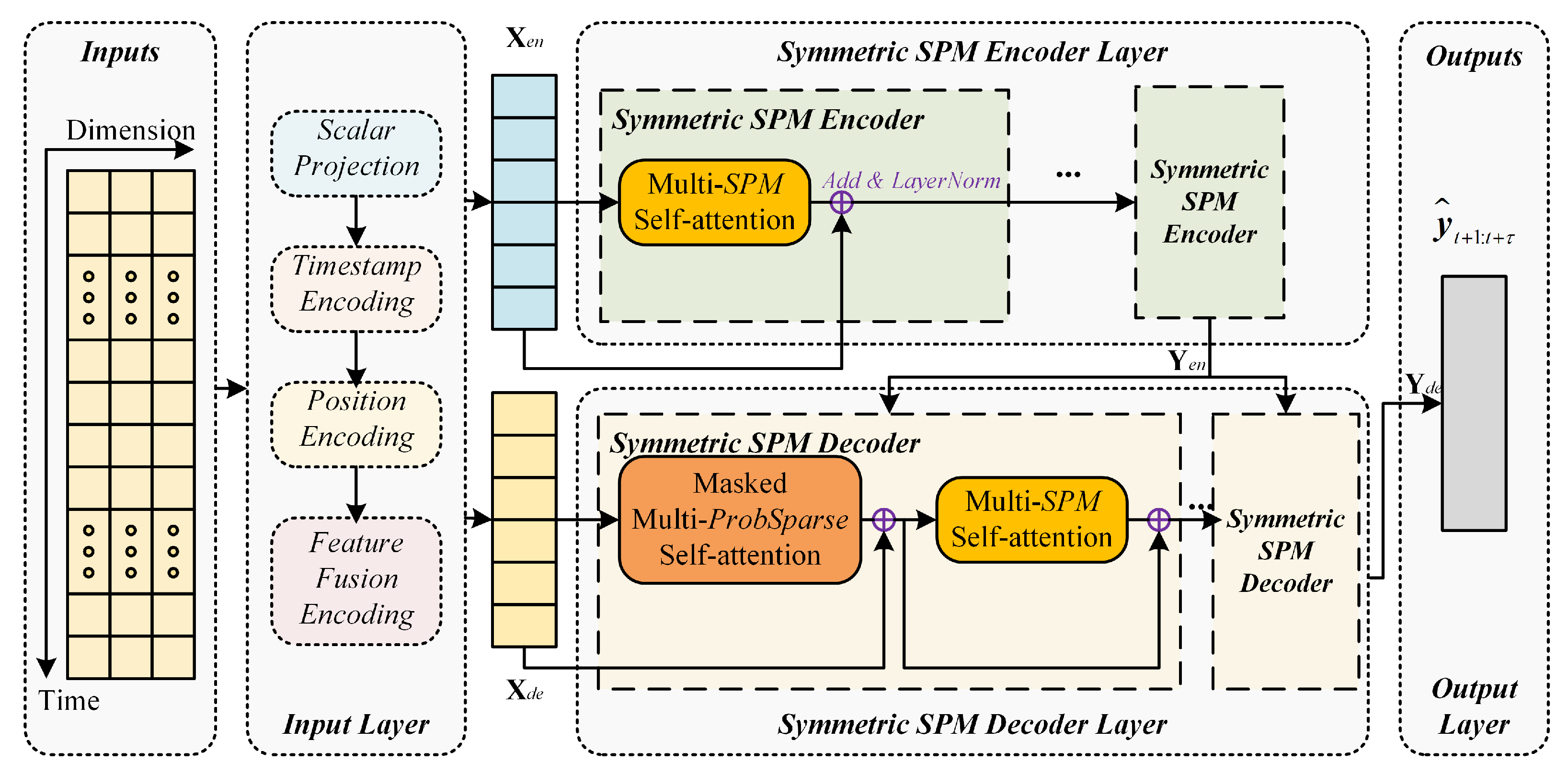
3.2. Overview of SPM

The overall architecture of the SPM-based method is shown in Figure 1. It is mainly divided into four parts: Input Layer, Symmetric SPM Encoder Layer, Symmetric SPM Decoder Layer, and Output Layer.

(1)

Input Layer

The Input Layer preprocesses the input features, which include target variables, covariates, and timestamp features. The input layer fuses discrete, continuous, and position encoding features and maps to the Symmetric SPM Encoder Layer input ${\mathbf{X}}_{en}$ and the Symmetric SPM Decoder Layer input ${\mathbf{X}}_{de}$, respectively.

(2)

Symmetric SPM Encoder Layer

The Symmetric SPM Encoder Layer consists of a stack of M symmetric SPM encoders. The symmetric SPM encoder consists of the multi-head SPM self-attention layer and normalization layer, which are connected by a residual network. The input ${\mathbf{X}}_{en}$ outputs ${\mathbf{Y}}_{en}$ through the Symmetric SPM Encoder Layer. ${\mathbf{Y}}_{en}$ is the input of the Symmetric SPM Decoder Layer.

(3)

Symmetric SPM Decoder Layer

The Symmetric SPM Decoder Layer consists of a stack of N symmetric SPM decoders. The symmetric SPM decoder consists of a masked multi-head ProbSparse self-attention layer, a normalization layer, and a multi-head SPM self-attention layer. ${\mathbf{X}}_{de}$ and ${\mathbf{Y}}_{en}$ are jointly input to the Symmetric SPM Decoder Layer to generate the output ${\mathbf{X}}_{de}$, which is the input of the fully connected Output Layer.

(4)

Output Layer

The Output Layer is composed of a fully connected layer, and the output ${\mathbf{X}}_{de}$ of the Symmetric SPM Decoder Layer is feature-mapped through the fully connected layer, and the predicted network traffic target ${\widehat{\mathbf{y}}}_{t+1:t+\tau }$ is obtained.

3.3. Input Layer

The input layer uniformly processes network traffic and relative position features to obtain outputs ${\mathbf{X}}_{en}\in {\mathbb{R}}^{L\times D}$ and ${\mathbf{X}}_{de}\in {\mathbb{R}}^{L\times D}$ (D and L are the dimensions of the data). These outputs are input into the SPM Encoder Layer and the SPM Decoder Layer.

3.3.1. Data Normalization

In order to avoid the interference of the experimental results of the model due to the large difference in the value of SMS, Call, and Internet, we utilize the min-max method to normalize the original sequence values to $[0,1]$.

$$z^{*}=\frac{z-z_{min}}{z_{max}-z_{min}},$$

(2)

where z is the original data value and $z^{*}$ is the data value after normalization (e.g., $y_i$ and $x_{i,j}$).

3.3.2. Scalar Projection

Scalar projection is used to project the input variable into a feature matrix. The normalized time series ${\mathbf{y}}_{1:t},{\mathbf{x}}_{1:t}$ are spliced to form the original variable matrix, they are projected as variable features ${\mathbf{X}}_{var}\in {\mathbb{R}}^{D\times (L+L_{token})}$ through the $Conv1D$ layer. In relative chronological order, the first ${\mathbf{X}}_{var}^{en}\in {\mathbb{R}}^{D\times L}$ is the partial input of the encoder, and the latter ${\mathbf{X}}_{var}^{de}\in {\mathbb{R}}^{D\times L_{token}}$ is the partial input of the decoder.

3.3.3. Timestamp Feature Encoding

Features such as dates and festivals (day, weekday, and month) are discrete category attribute features and cannot be directly used for model input. Therefore, it needs to be converted into vector form through the encoding layer. We adopt the embedding layer to encode the timestamp external features and convert the date-time features ${\mathbf{u}}_{i,1:t+\tau }$ into timestamp features ${\mathbf{X}}_{date}\in {\mathbb{R}}^{D\times L}$.

3.3.4. Position Encoding

When the historical sequence is input to the attention layer, all features are processed at the same time, without timing position information. Positional encoding is based on sine and cosine functions of different frequencies. By embedding the temporal relationship of the sequence, the positional encoding output ${\mathbf{X}}_{pos}\in {\mathbb{R}}^{D\times L}$ can be obtained.

3.3.5. Input Feature Fusion Encoding

The input ${\mathbf{X}}_{en}\in {\mathbb{R}}^{L\times D}$ of the SPM Encoder layer consists of variable feature ${\mathbf{X}}_{var}^{en}$, timestamp feature ${\mathbf{X}}_{date}$, and position encoding feature ${\mathbf{X}}_{pos}$.

$${\mathbf{X}}_{en}={({\mathbf{X}}_{var}^{en}+{\mathbf{X}}_{date}+{\mathbf{X}}_{pos})}^T$$

(3)

The input ${\mathbf{X}}_{en}\in {\mathbb{R}}^{L\times D}$ of the SPM decoding layer is mainly composed of a partial variable feature ${\mathbf{X}}_{var}^{de}$ with a length of $L_{token}$, a variable ${\mathbf{X}}_0\in {\mathbb{R}}^{D\times \tau }$ to be predicted with all zeros, and a timestamp feature ${\mathbf{X}}_{date}$. Masked multi-head attention is applied to the predicted location to avoid future information leakage.

$${\mathbf{X}}_{de}={(concat({\mathbf{X}}_{var}^{de},{\mathbf{X}}_0)+{\mathbf{X}}_{date})}^T$$

(4)

3.4. Symmetric SPM Encoder Layer

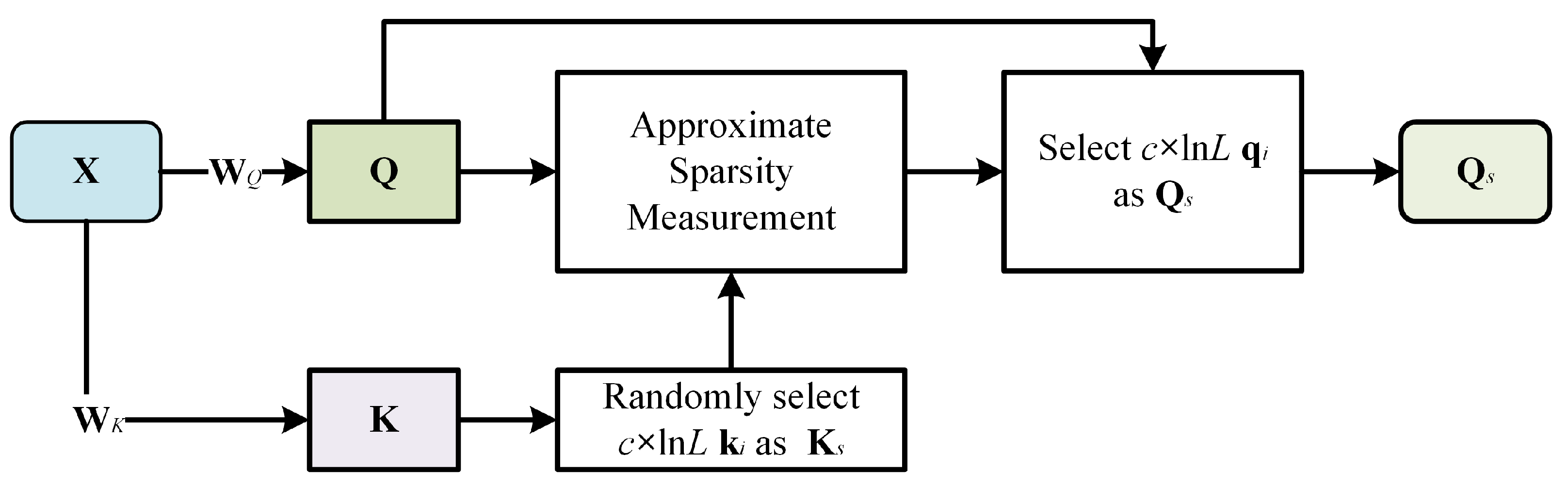
3.4.1. Sparse Query Block

By focusing and persistently memorizing key features related to NTP, the SPM self-attention utilizes less key attention, reduces complexity, and achieves better prediction results. The SPM self-attention layer leverages the Sparse Query Block to decrease the complexity and remain the effect in some case [30]. The calculation process of Sparse Query Block is shown in Figure 2, where $\mathbf{X}\in {\mathbb{R}}^{L\times D}$ denotes the input, query matrices $\mathbf{Q}=\mathbf{X}{\mathbf{W}}_{{}^Q}$, key matrices $\mathbf{K}=\mathbf{X}{\mathbf{W}}_{{}^K}$, and value matrices $\mathbf{V}=\mathbf{X}{\mathbf{W}}_{{}^V}$ respectively. The calculating progress of Sparse Query Block can be formulated as follows.

First, we evaluate the sparsity of ${\mathbf{q}}_i$ through the computational formulation that empirically approximates the sparsity.

$$\overline{M}({\mathbf{q}}_i,\mathbf{K})=\underset{j}{max}\left\{\frac{{\mathbf{q}}_i{\mathbf{k}}_j^T}{\sqrt{d_k}}\right\}-\frac{1}{L_K}\sum _{j=1}^{L_K}\frac{{\mathbf{q}}_i{\mathbf{k}}_j^T}{\sqrt{d_k}},$$

(5)

where ${\mathbf{q}}_i$ is the row vector of $\mathbf{Q}\in {\mathbb{R}}^{L_Q\times d_k}$, and ${\mathbf{k}}_i$ is the row vector of $\mathbf{K}\in {\mathbb{R}}^{L_K\times d_k}$.

We randomly sample $c\times log{L}_K$${\mathbf{k}}_i$ vectors as ${\mathbf{K}}_s$ (c is the sampling constant), and calculate the sparsity of all ${\mathbf{q}}_i$ and ${\mathbf{K}}_s$ in $\mathbf{Q}$ through the sparsity calculation formula, and obtain the sparsity set $M_s$.

$$M_s=\left\{\overline{M}({\mathbf{q}}_1,{\mathbf{K}}_s),\overline{M}({\mathbf{q}}_2,{\mathbf{K}}_s),\cdots ,\overline{M}({\mathbf{q}}_{L_Q},{\mathbf{K}}_s)\right\}$$

(6)

Then, we utilize the $top$-k function to sort and filter $M_s$ to obtain the first $k=c\times log{L}_Q$ subscript sets S corresponding to the sparsity.

$$S=topk\left(M_s\right)=\{s_1,s_2\cdots ,s_k\}$$

(7)

Finally, the sparse ${\mathbf{Q}}_s$ is obtained by filtering from $\mathbf{Q}$ through the subscript set S.

$${\mathbf{Q}}_s=\left[\begin{array}{c}{\mathbf{q}}_1\\ {\mathbf{q}}_2\\ ⋮\\ {\mathbf{q}}_{L_Q}\end{array}\right],{}^{}{\mathbf{q}}_i=\left\{\begin{array}{cc}{\mathbf{q}}_i,& i\in S,1\le i\le L_Q\\ \mathbf{0},& i\notin S,1\le i\le L_Q\end{array},\right.$$

(8)

where ${\mathbf{Q}}_s$ is a sparse matrix of the same-size as $\mathbf{Q}$, and it only consists of $c\times log{L}_Q$ valid query vectors (non-zero vector) under the sparsity measurement.

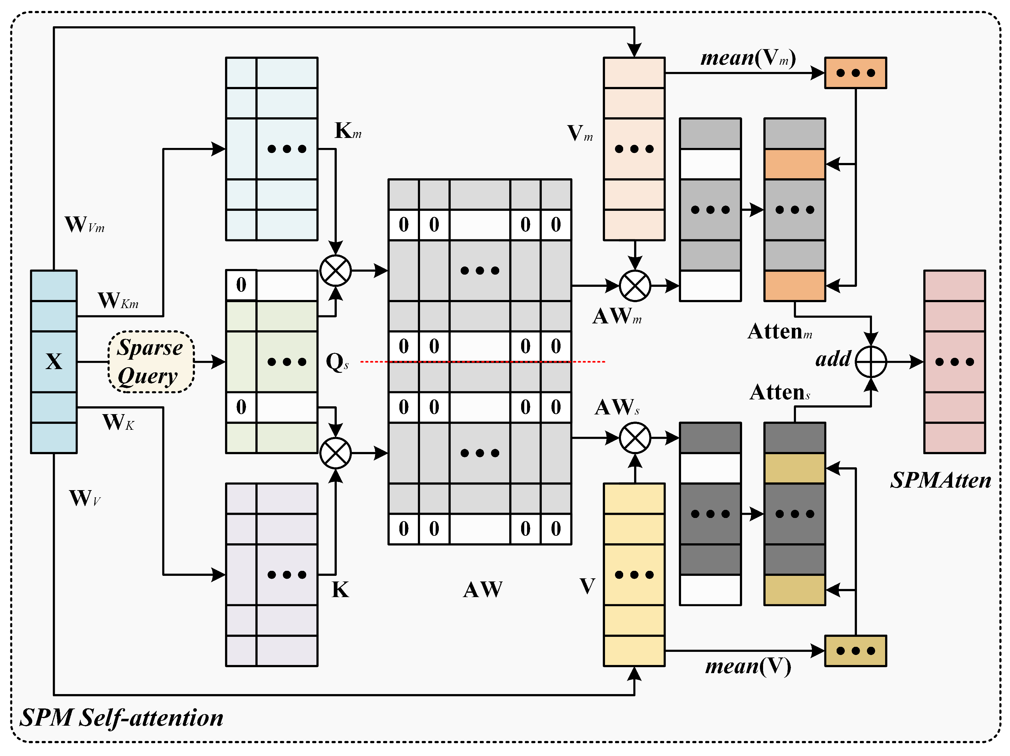
3.4.2. SPM Self-Attention

Based on sparse query ${\mathbf{Q}}_s$, the SPM self-attention layer is shown in Figure 3, where $\mathbf{X}\in {\mathbb{R}}^{L\times D}$ denotes the input, query matrices $\mathbf{Q}=\mathbf{X}{\mathbf{W}}_Q$, key matrices ${\mathbf{K}}_m=\mathbf{X}{\mathbf{W}}_{Km}$, and value matrices ${\mathbf{V}}_m=\mathbf{X}{\mathbf{W}}_{Vm}$ respectively. ${\mathbf{Q}}_s$ is a sparse query, which can be obtained through the Sparse Query Block. The calculating progress of SPM self-attention (SPMAtten) can be formulated as follows.

(1)

Concatenation and normalization of sparse key attention weights

${\mathbf{Q}}_s$ is used as a connection bridge between newly added ${\mathbf{K}}_m\in {\mathbb{R}}^{L_K\times d_k}$ and $\mathbf{K}\in {\mathbb{R}}^{L_K\times d_k}$, and the attention weight Sim is obtained by concatenating the matrix dot product results. After that, the Sim is scaled by $\sqrt{d_k}$, and the normalized attention weight (AW) is calculated by the $softmax$ layer. The $softmax$ is one of the core components of Transformer, which helps to capture long-range dependencies and thus improves the prediction performance of the attention-based methods [28].

$$Sim({\mathbf{Q}}_s,\mathbf{K},{\mathbf{K}}_m)=concat({\mathbf{Q}}_s{\mathbf{K}}^T,{\mathbf{Q}}_s{\mathbf{K}}_m^T)$$

(9)

$$AW=softmax\left(Sim/\phantom{Sim\sqrt{d_k}}\sqrt{d_k}\right)$$

(10)

(2)

Split and fill sparse attention

$AW$ contains all network traffic key attention weight information. Firstly, we split the attention weights of $AW\in {\mathbb{R}}^{L_Q\times (L_K+l_k)}$ to get $A{W}_s\in {\mathbb{R}}^{L_Q\times L_K}$ and $A{W}_m\in {\mathbb{R}}^{L_Q\times l_K}$. The new attention weight $A{W}_m$ has a persistent memory for key features. We calculate the dot product of the split attention weight with $\mathbf{V}\in {\mathbb{R}}^{L_V\times d_v}$ and the newly added ${\mathbf{V}}_m\in {\mathbb{R}}^{l_V\times d_v}$, respectively, to obtain the key attention values of $Atte{n}_s^{\prime }\in {\mathbb{R}}^{L_Q\times d_v}$ and $Atte{n}_m^{\prime }\in {\mathbb{R}}^{L_Q\times d_v}$. $Atte{n}_m^{\prime }$ is the key attention value that persistently memorizes the new attention layer of the network traffic features.

$$Atte{n}_s^{\prime }=A{W}_s·\mathbf{V}$$

(11)

$$Atte{n}_m^{\prime }=A{W}_m·{\mathbf{V}}_m$$

(12)

Then, we fill and complete the attention value of the corresponding positions of the $L_Q-c\times log{L}_Q$ zero vectors in ${\mathbf{Q}}_s$ to obtain secondary filling attentions $Atte{n}_s^{″}$ and $Atte{n}_m^{″}$. The fill value is the vector $\mathbf{v}\in {\mathbb{R}}^{d_v}$ and ${\mathbf{v}}_m\in {\mathbb{R}}^{d_v}$ composed of the average value of $\mathbf{V}$ and ${\mathbf{V}}_m$, respectively. Finally, the secondary attention and the key attention are combined respectively to obtain two parts of attention $Atte{n}_s$ and $Atte{n}_m$.

$$Atte{n}_s({\mathbf{Q}}_s,\mathbf{K},\mathbf{V})=\{Atte{n}_s^{\prime },Atte{n}_s^{″}\}$$

(13)

$$Atte{n}_m({\mathbf{Q}}_s,{\mathbf{K}}_m,{\mathbf{V}}_m)=\{Atte{n}_m^{\prime },Atte{n}_m^{″}\}$$

(14)

(3)

Fusion sparse key attention

Finally, we superimpose the key attention in $Atte{n}_s$ and $Atte{n}_m$, and act together on the output of the attention to obtain the fusion sparse key attention, that is, the output of the SPM self-attention layer ($SPMAtten$).

$$SPMAtten({\mathbf{Q}}_s,\mathbf{K},{\mathbf{K}}_m,\mathbf{V},{\mathbf{V}}_m)=Atte{n}_s+Atte{n}_m$$

(15)

(4)

Multi-head SPM self-attention layer

The self-attention generally appears in the form of multi-head attention. Each attention head performs the attention function in parallel to generate the output values of h attention heads, and these attention heads, calculated with different sparse key-value pairs, are used. The output values are spliced together and projected through the projection matrix ${\mathbf{W}}_{{}^O}\in {\mathbb{R}}^{h{d}_v\times D}$ for which to obtain the output result of the multi-head SPM self-attention (MSPMAtten).

$$\begin{array}{cc}\hfill MSPMAtten\left(\mathbf{X}\right)& \hfill =MultiHead(\mathbf{Q},\mathbf{K},{\mathbf{K}}_m,\mathbf{V},{\mathbf{V}}_m)\hfill \\ \hfill & \hfill =concat(hea{d}_1,\cdots ,hea{d}_h){\mathbf{W}}_{{}^O},\hfill \end{array}$$

(16)

$$hea{d}_i=SPMAtten({\mathbf{Q}}_i,{\mathbf{K}}_i,{\mathbf{K}}_{m_i},{\mathbf{V}}_i,{{\mathbf{V}}_m}_{{}_i}),$$

(17)

where ${\mathbf{Q}}_i\in {\mathbb{R}}^{L\times d_k}$, ${\mathbf{K}}_i\in {\mathbb{R}}^{L\times d_k}$, ${\mathbf{K}}_{m_i}\in {\mathbb{R}}^{l\times d_k}$, ${\mathbf{V}}_i\in {\mathbb{R}}^{L\times d_v}$, ${\mathbf{V}}_{m_i}\in {\mathbb{R}}^{l\times d_v}$, h is the number of attention heads, in this work, $d_k=d_v=d$.

3.4.3. Symmetric SPM Encoder Layer

The symmetric SPM encoder is mainly composed of a multi-head SPM self-attention and a normalization layer, which are connected by a residual network structure. The X input to the symmetric SPM encoder, and the output ${\mathbf{h}}_i$ of the i-th encoder are obtained, which can be expressed as follows.

$$\begin{array}{l}{\mathbf{h}}_i=SPMEncoder\left(\mathbf{X}\right)\\ =\mathbf{X}+LayerNorm\left(MSPMAtten\right(\mathbf{X}\left)\right)\end{array}$$

(18)

The Symmetric SPM Encoder Layer is formed by stacking M symmetric SPM encoders. ${\mathbf{X}}_{en}$ is input to the Symmetric SPM Encoder Layer, and the network traffic encoding feature ${\mathbf{Y}}_{en}$ after the Symmetric SPM Encoder Layer is stacked with M layers of symmetric SPM encoders, which can be formally defined as follows.

$${\mathbf{h}}_i^{en}=\left\{\begin{array}{cc}SPMEncoder\left({\mathbf{X}}_{en}\right),& i=1\\ SPMEncoder\left({\mathbf{h}}_{i-1}^{en}\right),& 2\le i\le M\end{array},\right.$$

(19)

$${\mathbf{Y}}_{en}={\mathbf{h}}_M^{en}=SPMEncoder\left({\mathbf{h}}_{M-1}^{en}\right)$$

(20)

3.5. Symmetric SPM Decoder Layer

3.5.1. ProbSparse Self-Attention

The ProbSparse self-attention evaluates the main attention in the input features of network traffic by sparsity. The input $\mathbf{X}\in {\mathbb{R}}^{L\times D}$ first gets ${\overline{\mathbf{Q}}}_s$ through the Sparse Query Block and then obtains the masked ProbSparse self-attention (MPSAtten) through the dot product.

$$MPSAtten({\overline{\mathbf{Q}}}_s,\overline{\mathbf{K}},\overline{\mathbf{V}})=softmax\left(\frac{{\overline{\mathbf{Q}}}_s{\overline{\mathbf{K}}}^T}{\sqrt{d_k}}·\mathbf{M}\right)\overline{\mathbf{V}},$$

(21)

where $\overline{\mathbf{Q}}=\mathbf{X}{\mathbf{W}}_{{}^{\overline{Q}}},\overline{\mathbf{K}}=\mathbf{X}{\mathbf{W}}_{{}^{\overline{K}}},\overline{\mathbf{V}}=\mathbf{X}{\mathbf{W}}_{{}^{\overline{V}}}$, the dimensions of ${\overline{\mathbf{Q}}}_s$ and $\overline{\mathbf{Q}}$ are the same, with the difference being that the number of effective vectors of ${\overline{\mathbf{Q}}}_s$ is $c\times lnL$, c is the constant sampling factor, and M is the mask matrix used to avoid future information leakage. The masked multi-head ProbSparse self-attention (MMPSAtten) can be formally defined as follows.

$$\begin{array}{ll}MMPSAtten\left(\mathbf{X}\right)& =MultiHead({\overline{\mathbf{Q}}}_s,\overline{\mathbf{K}},\overline{\mathbf{V}})\\ & =concat(hea{d}_1,\cdots ,hea{d}_h){\mathbf{W}}_{{}^{\overline{O}}},\end{array}$$

(22)

$$hea{d}_i=MPSAtten({\overline{\mathbf{Q}}}_{s_i},{\overline{\mathbf{K}}}_i,{\overline{\mathbf{V}}}_i),$$

(23)

where ${\overline{\mathbf{Q}}}_{s_i}\in {\mathbb{R}}^{L\times d}$, ${\overline{\mathbf{K}}}_i\in {\mathbb{R}}^{L\times d}$, ${\overline{\mathbf{V}}}_i\in {\mathbb{R}}^{L\times d}$.

3.5.2. Symmetric SPM Decoder Layer

The symmetric SPM decoder is mainly composed of a MSPMAtten layer, a MMPSAtten layer, and a normalization layer, which are connected by two residual network structures. The input of the symmetric SPM decoder is divided into two parts, denoted as X and Y respectively. The input X passes through the MMPSAtten layer and outputs the sparse key attention value. Through the first layer normalization and residual connection, the intermediate output ${\mathbf{p}}_i$ of the i-th decoder is obtained.

$${\mathbf{p}}_i=\mathbf{X}+LayerNorm\left(MMPSAtten\left(\mathbf{X}\right)\right)$$

(24)

Then, ${\mathbf{p}}_i$ and another part of the input Y are jointly input into the multi-head SPM self-attention. Through the second layer normalization and residual connection, the output ${\mathbf{h}}_i$ of the i-th decoder is obtained, which can be expressed as follows.

$$\begin{array}{ll}{\mathbf{h}}_i& =SPMDecoder(\mathbf{X},\mathbf{Y})\\ & ={\mathbf{p}}_i+LayerNorm\left(MSPMAtten({\mathbf{p}}_i,\mathbf{Y})\right)\end{array}$$

(25)

The Symmetric SPM Decoder Layer is formed by stacking N symmetric SPM decoders. ${\mathbf{X}}_{de}$ and ${\mathbf{Y}}_{en}$ are input to the Symmetric SPM Decoder Layer. After stacking N layers of symmetric SPM decoders, the encoded features of the network traffic are decoded into the output ${\mathbf{Y}}_{de}$, which can be formally defined as follows.

$${\mathbf{h}}_i^{de}=\left\{\begin{array}{cc}SPMDecoder({\mathbf{X}}_{de},{\mathbf{Y}}_{en}),& i=1\\ SPMDecoder({\mathbf{h}}_{i-1}^{de},{\mathbf{Y}}_{en}),& 2\le i\le N\end{array},\right.$$

(26)

$${\mathbf{Y}}_{de}={\mathbf{h}}_N^{de}=SPMDecoder({\mathbf{h}}_{N-1}^{de},{\mathbf{Y}}_{en})$$

(27)

3.6. Output Layer

After passing through the Symmetric SPM Decoder Layer, the fully connected (FC) layer is used to extract features. The calculation process for the NTP target can be formally formulated as follows.

$$\begin{array}{c}{\widehat{\mathbf{y}}}_{t+1:t+\tau }={\mathbf{W}}_2\left(ReLU({\mathbf{W}}_1{\mathbf{Y}}_{de}+{\mathbf{b}}_1)\right)+{\mathbf{b}}_2,\end{array}$$

(28)

where ${\mathbf{W}}_1,{\mathbf{W}}_2,{\mathbf{b}}_1,$ and ${\mathbf{b}}_2$ are learnable parameters of the FC layer. ReLU denotes the activation function, and ${\widehat{\mathbf{y}}}_{t+1:t+\tau }$ is the NTP target.

3.7. Cost Function

The widely used exponential mean square error (MSE) is utilized as a cost function to calculate the errors of the ground truth and the predicted value [32].

$$MSE=\frac{1}{m}\sum _{i=1}^m{\left(y_i-\widehat{y_i}\right)}^2,$$

(29)

where $y_i$ and $\widehat{y_i}$ are the ground truth and predicted value of the network traffic, respectively. m denotes the total number of the training samples.

4. Evaluation

4.1. Dataset Description and Experiment Setup

4.1.1. Dataset Description

The evaluation dataset is an openly accessible multi-source dataset of the Telecom Italia Big Data Challenge [33], which is widely used in NTP evaluation. The dataset consists of a time series of traffic from 1 November 2013 to 1 January 2014 in Milan and Trentino, with an interval of 10 min. This dataset records five main types of activity data attributes, including Received SMS, Sent SMS, Incoming Call, Outgoing Call, and Internet. As the statement in Problem Formulation, the Internet attribute is the target predicted variable, and the other variables are the covariates associated with the target Internet.

4.1.2. Experiment Setup

The experimental data preprocessing strategy is performed as follows. We combine the receive and send dimensions and adopt the preprocessing measures by inputting the total traffic in the prediction model. All data are pre-processed by min-max normalization, which allows the model to converge faster and improves the computational efficiency of the fitting process, thus benefiting the accurate NTP [19]. A total of 80% of the historical data is applied as the training dataset and the remaining 20% is applied as the test dataset. To avoid overfitting in training, we randomly divide part data from the training set as the validation set. All the datasets are constructed using the widely used sliding window method [20].

The hyperparameter settings of the SPM model and its variants are as follows. The number of symmetric SPM Encoder and Decoder is 3 and the number of attention heads is 4. Moreover, the Adam [34] optimizer is adopted, the initial learning rate is set to 0.02, the batch size is 32, and the number of training iterations is 300.

4.1.3. Evaluated Approaches and Metrics

We implement the following baseline approaches.

• ARIMA [11], or autoregressive integrated moving average model, is one of the most classic time series prediction models;
• LSTM [35], or long short-term memory, is an extension of the RNN model;
• GRU [16], or gated recurrent unit, is a variant of LSTM;
• DeepAR [27] is a probabilistic prediction model based on neural networks, and its prediction target is the probability distribution of sequences over time steps;
• Transformer [20] is an improved prediction model based on vanilla Transformer.

To evaluate the NTP accuracy of these approaches, we adopt three metrics to evaluate the NTP accuracy, i.e., the root mean square error (RMSE), mean absolute error (MAE), and determination coefficient $R^2$. Their calculation formulas are given as

$$RMSE=\sqrt{\frac{1}{n}\sum _{i=1}^n{\left(y_i-\widehat{y_i}\right)}^2},$$

(30)

$$MAE=\frac{1}{n}\sum _{i=1}^n\left|y_i-\widehat{y_i}\right|,$$

(31)

$$R^2=1-\frac{{\displaystyle \sum _{i=1}^n}{(y_i-{\widehat{y}}_i)}^2}{{\displaystyle \sum _{i=1}^n}{(y_i-\overline{y})}^2},$$

(32)

where $y_i$ and $\widehat{y_i}$ are the ground truth and predicted value of network traffic, respectively. $\overline{y}$ is the average values of the ground truth. n is the length of the sequence to be predicted.

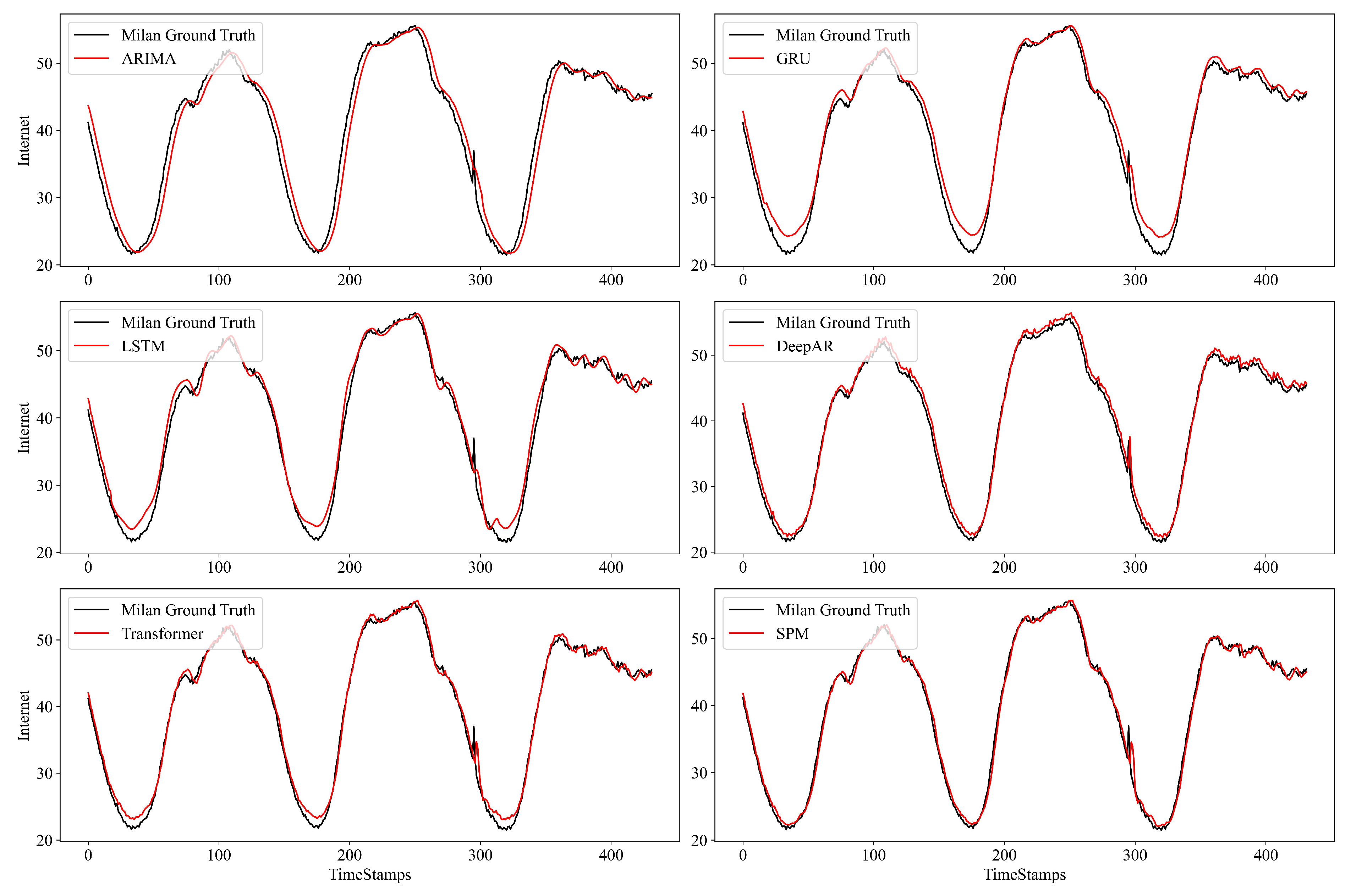
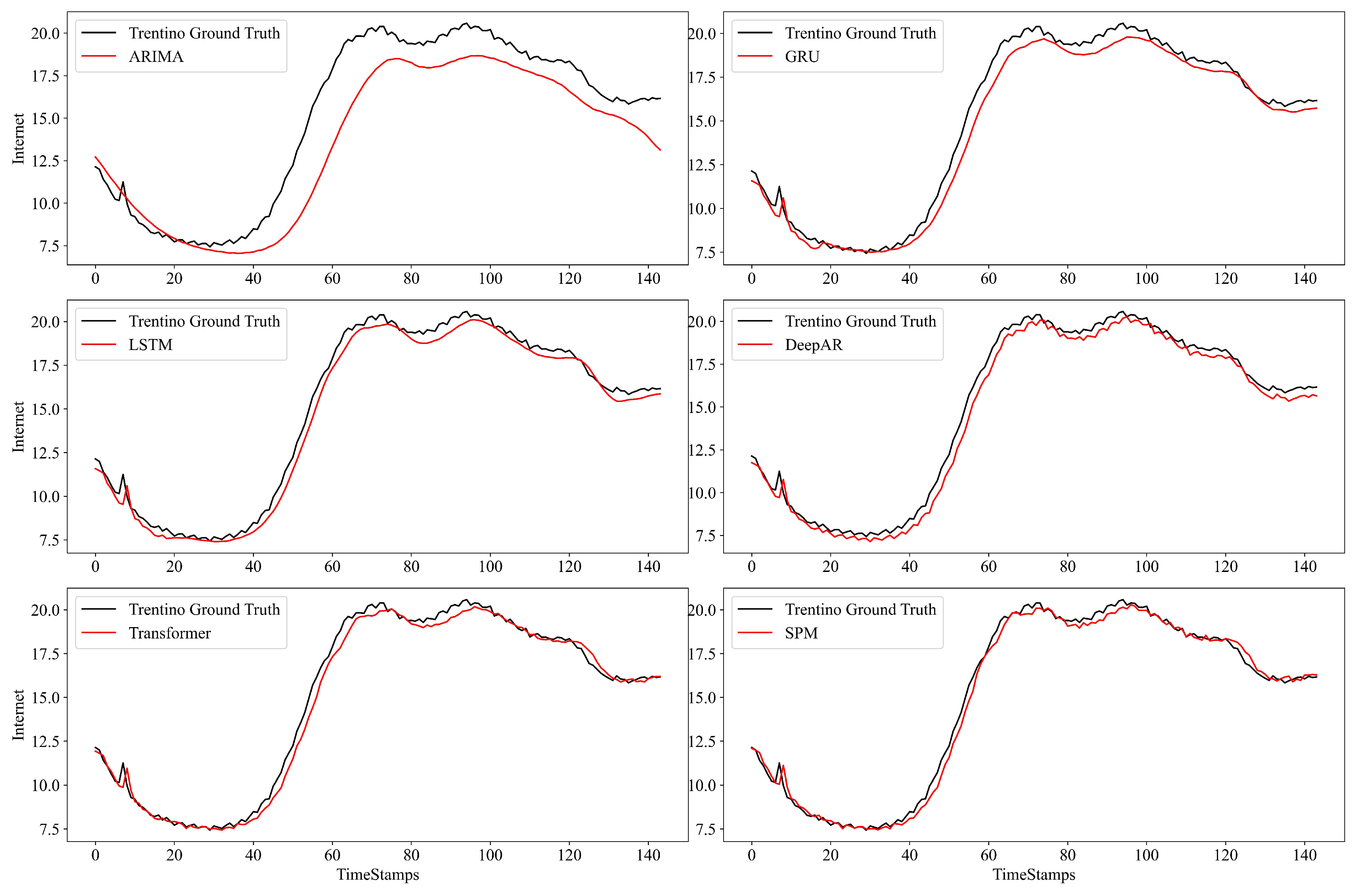
4.2. Evaluation Results

Table 2. Experimental results of RMSE ($\times {10}^{-2}$) on the Milan dataset.

Methods	$\mathit{\tau }$ = 144	$\mathit{\tau }$ = 432	$\mathit{\tau }$ = 1008
ARIMA	190.1470	196.6632	206.1349
GRU	99.6861	150.1390	142.0568
LSTM	107.0977	131.5001	152.1568
DeepAR	89.4358	74.2318	87.7861
Transformer	79.8580	87.7893	126.4511
SPM	49.1054	58.4251	67.1300

Bolded indicates the optimal value, underlined denotes sub-optimal value.

,

Table 3. Experimental results of MAE on the Milan dataset.

Methods	$\mathit{\tau }$ = 144	$\mathit{\tau }$ = 432	$\mathit{\tau }$ = 1008
ARIMA	1.3847	1.5369	1.6408
GRU	0.7939	1.1959	1.1203
LSTM	0.8931	1.0615	1.1814
DeepAR	0.5981	0.5570	0.6963
Transformer	0.6378	0.6637	0.9250
SPM	0.3839	0.3785	0.4782

Bolded indicates the optimal value, underlined denotes sub-optimal value.

,

Table 4. Experimental results of $R^2$ on the Milan dataset.

Methods	$\mathit{\tau }$ = 144	$\mathit{\tau }$ = 432	$\mathit{\tau }$ = 1008
ARIMA	0.8777	0.8249	0.8128
GRU	0.9163	0.8803	0.7832
LSTM	0.9546	0.8183	0.8365
DeepAR	0.9790	0.9546	0.9177
Transformer	0.9849	0.8072	0.6995
SPM	0.9901	0.9630	0.9578

Bolded indicates the optimal value, underlined denotes sub-optimal value.

,

Table 5. Experimental results of RMSE ($\times {10}^{-2}$) on the Trentino dataset.

Methods	$\mathit{\tau }$ = 144	$\mathit{\tau }$ = 432	$\mathit{\tau }$ = 1008
ARIMA	89.1283	112.846	120.8139
GRU	73.7290	93.2989	130.0032
LSTM	54.3140	114.9338	112.9086
DeepAR	36.9362	57.4856	80.1257
Transformer	31.3617	118.3934	153.0669
SPM	25.4240	51.8640	57.3931

Bolded indicates the optimal value, underlined denotes sub-optimal value.

,

Table 6. Experimental results of MAE on the Trentino dataset.

Methods	$\mathit{\tau }$ = 144	$\mathit{\tau }$ = 432	$\mathit{\tau }$ = 1008
ARIMA	0.6029	0.7877	0.8477
GRU	0.5470	0.6848	0.9567
LSTM	0.4299	0.8825	0.7772
DeepAR	0.2453	0.3924	0.6811
Transformer	0.2356	0.8722	0.9705
SPM	0.1933	0.3794	0.3902

Bolded indicates the optimal value, underlined denotes sub-optimal value.

and

Table 7. Experimental results of $R^2$ on the Trentino dataset.

Methods	$\mathit{\tau }$ = 144	$\mathit{\tau }$ = 432	$\mathit{\tau }$ = 1008
ARIMA	0.8612	0.7758	0.7344
GRU	0.9050	0.8467	0.6924
LSTM	0.9485	0.7674	0.7680
DeepAR	0.9762	0.9418	0.8832
Transformer	0.9829	0.7532	0.5736
SPM	0.9887	0.9527	0.9401

Bolded indicates the optimal value, underlined denotes sub-optimal value.

demonstrate the comparison results of SPM and baseline methods on two datasets, respectively. From the table, three observations can be found.

(1)

The performance of the classical model (e.g., ARIMA) is generally lower than that of the NN-based approaches, because such classical approaches generally rely on the mean value of history;

(2)

Transformer has effective performance when the prediction step is short ($\tau$ = 144). However, as the prediction step increases ($\tau$ = 432, 1008), the Transformer pays attention to all the features. It will generate a quadratic complexity, causing its inference speed to be slow. In addition, the key attention feature will also be affected by most other non-critical attention features, resulting in performance degradation, which is lower than the DeepAR;

(3)

SPM can decrease the interference of other non-critical attention information and focus on more key attention information, which can effectively improve the prediction performance. For instance, on the Milian dataset ($\tau$ = 1008), SPM achieves RMSE reductions of 52.7%, 55.9%, and 23.5%, compared with GRU, LSTM, and DeepAR respectively. Moreover, compared with Transformer, SPM reduces the prediction MAE and RMSE by 48.3% and 42.9%, respectively. When measured by $R^2$, the average $R^2$ of SPM at different prediction steps is about 0.1142 and 0.1553 higher than the sub-optimal baseline in the two datasets, respectively.

The NTP results are illustrated in Figure 4 and Figure 5. We plot NTP results for $\tau$ = 432 on Milan and $\tau$ = 144 on Trentino datasets, with similar results for other prediction steps. It can be seen that SPM can achieve the optimal NTP accuracy with respect to the baseline approaches. On average, when measured by MAE, SPM outperforms the sub-optimal method by 33.0% and 21.3% in two datasets respectively.

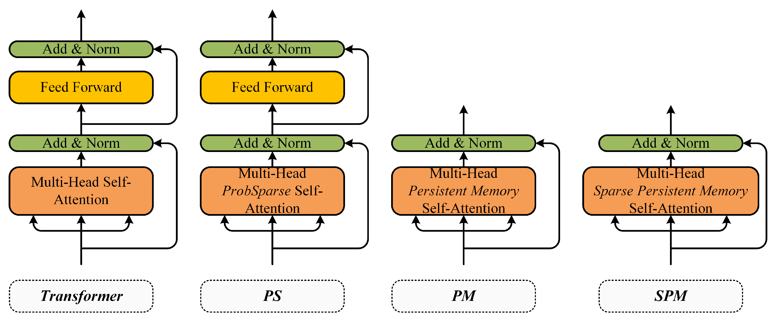
4.3. Ablation Evaluation

To further verify the temporal performance of SPM, the ablation baselines are tested in the same experimental environment. The encoder architecture of the ablation methods are demonstrated in Figure 6.

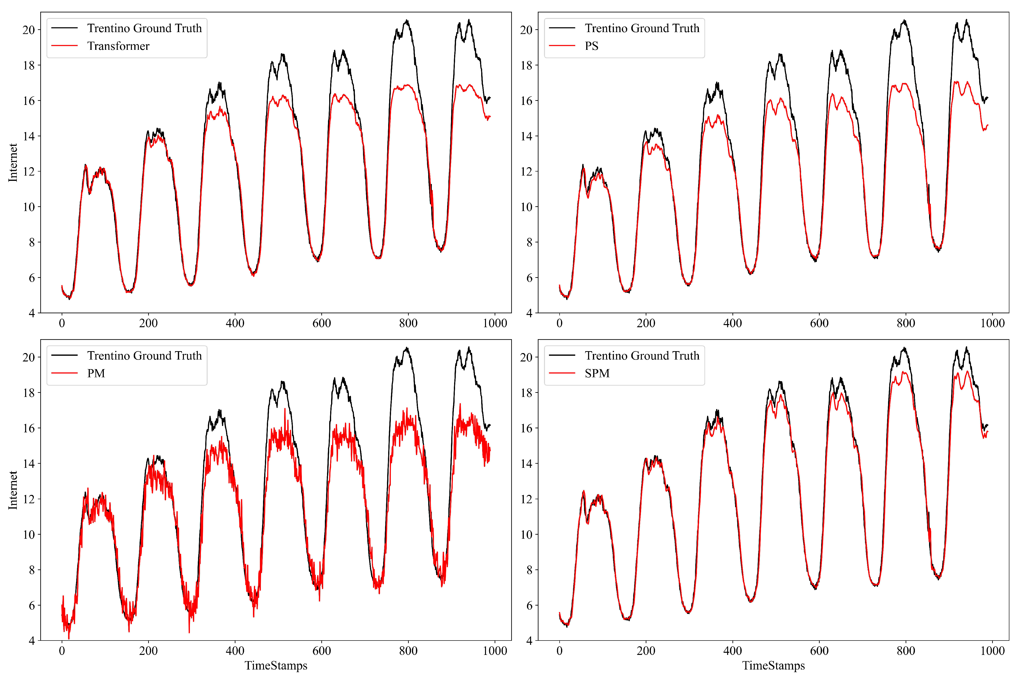
• Transformer, an improved prediction model based on vanilla Transformer;
• PS, or ProbSparse Transformer, Ablation model, using the ProbSparse self-attention layer to replace the vanilla self-attention layer;
• PM, or Persistent Memory Transformer, Ablation model, using the persistent memory self-attention layer structure, removing the feed-forward sub-layer;
• SPM, the proposed symmetric model in this paper.

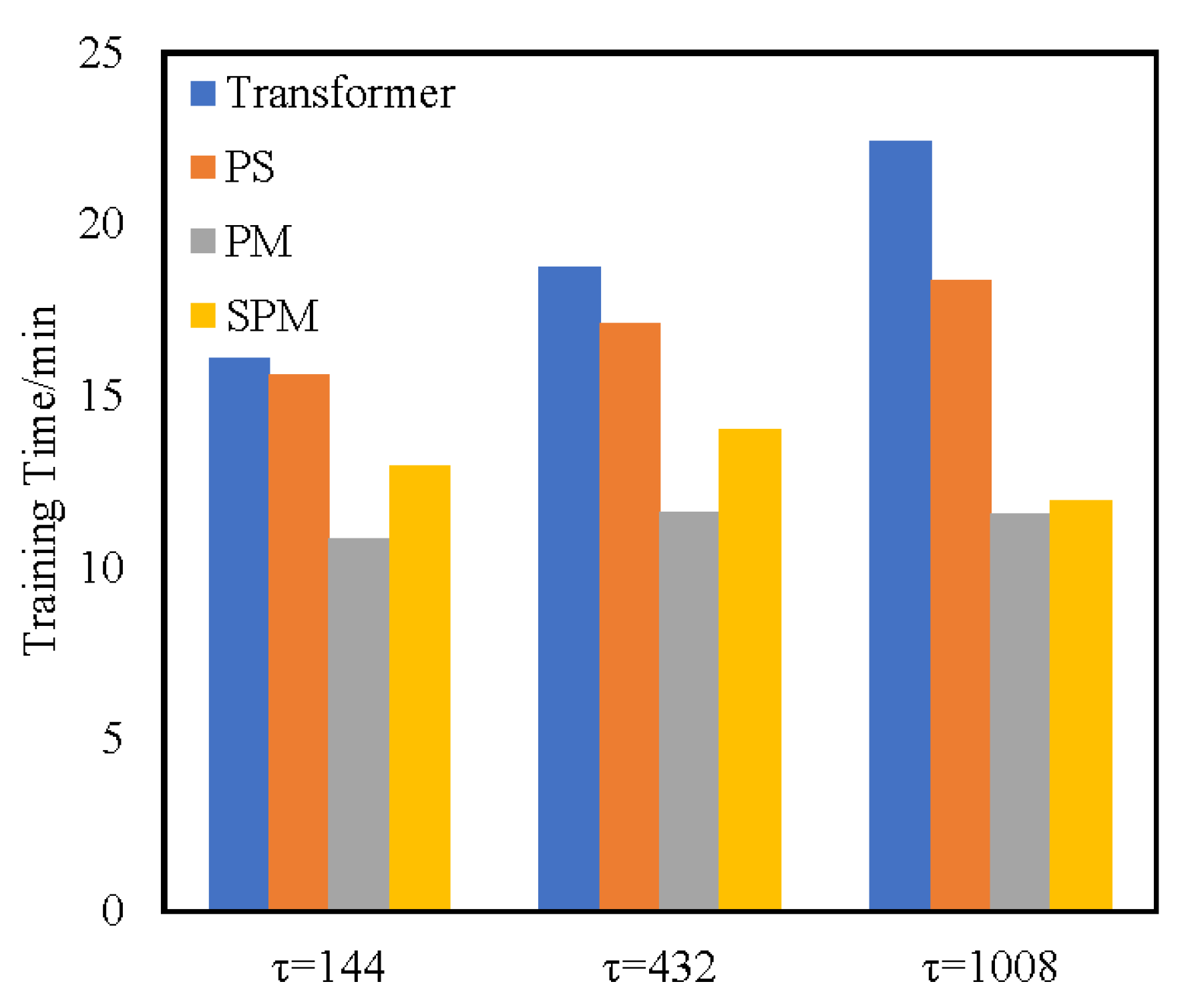
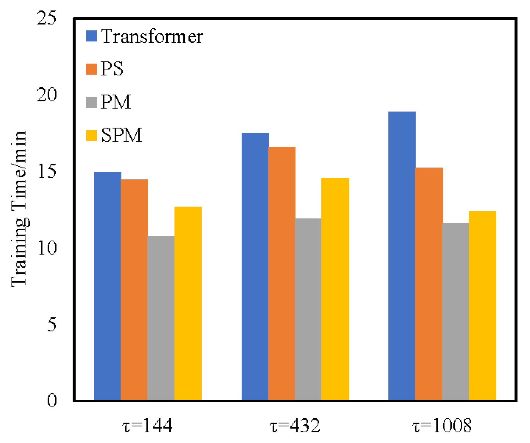
4.3.1. Time Complexity Analysis

The SPM is an improvement based on the vanilla Transformer. The existing work mainly analyzes the time complexity of the two main parts, which includes the self-attention layer and the feed-forward layer. The vanilla Transformer has both $O\left(L^{2}d\right)$ in two parts [29]. The PS adopts the ProbSparse self-attention layer, and the complexity of the self-attention part is $O(LdlogL)$ [30]. The PM removes the feed-forward layer, and the complexity of feed-forward is $O\left(0\right)$ [31]. In the sparse persistent memory self-attention layer, the SPM adopts the sparse query $\mathbf{Q}s$ to calculate the self-attention, the complexity is $O(max(L,l)dlogL)$. Moreover, in the feed-forward layer, the SPM removes the feed-forward, and thus the complexity is $O\left(0\right)$. The complexity comparison results are shown in

Table 8. Comparison of the time complexity.

Model	Self-Attention Layer	Feed-Forward Layer
Transformer	$O\left(L^{2}d\right)$	$O\left(L^{2}d\right)$
PS	$O(LdlogL)$	$O\left(L^{2}d\right)$
PM	$O\left(L^{2}d\right)$	$O\left(0\right)$
SPM	$O\left(\max \right(L,l)dlogL)$	$O\left(0\right)$

, where l is the dimension of the added attention layer.

4.3.2. Ablation Evaluation Results of Temporal Performance

The temporal experimental results are demonstrated in Figure 7 and Figure 8. From the figure, three observations can be found.

(1)

The PS Transformer replaces the vanilla attention layer with the ProbSparse self-attention layer. In terms of time performance, the complexity of the ProbSparse self-attention layer has been proved to be lower than that of the original attention layer. Therefore, the training time of the PS Transformer model is shorter than that of the Transformer model.

(2)

PM Transformer adopts the structure of the PM self-attention layer, which eliminates the feed-forward sub-layer and has low complexity. In terms of time performance, although the complexity of the self-attention layer is $O\left(L^{2}d\right)$, the calculation method of self-attention is direct and does not calculate other factors. Therefore, the training time of PM is lower than that of SPM models.

(3)

SPM utilizes the SPM self-attention layer to obtain key attention information in the form of a sparse query matrix and carries out persistent memory for key attention information to retain the key attention information in a new attention layer. When calculating SPM attention, two attention fragments are calculated by branches and the attention weight is concatenated. Although such a fragmented structure has been shown to be beneficial for accuracy, it could decrease the efficiency because it is unfriendly for devices with strong parallel computing powers such as GPU. It also introduces extra overheads such as kernel launching and synchronization [36]. However, PM uses a simple single-branch calculation method, which can fully make use of the parallel computing powers of GPU and has high training efficiency. Thus, although the theoretical time complexity of SPM has reached a good level, the actual training time may be longer than that of PM. Compared with other methods, SPM removes the high complexity component of the feed-forward layer, and thus the time performance is in sub-optimal performance. Compared with Transformer, the training time of SPM is reduced by 22.2% and 30.4% on two real-world datasets, respectively. Compared with the baseline approaches, the $R^2$ evaluation metric is also optimal on two datasets.

4.3.3. Ablation Evaluation Results of Prediction Performance

The experimental results are demonstrated in

Table 9. Ablation experimental results of RMSE ($\times {10}^{-2}$) on the Milan dataset.

Methods	$\mathit{\tau }$ = 144	$\mathit{\tau }$ = 432	$\mathit{\tau }$ = 1008
Transformer	79.8580	87.7893	126.4511
PS	84.8511	92.1521	117.6370
PM	112.8224	136.8528	162.4517
SPM	49.1054	58.4251	67.1300

Bolded indicates the optimal value, underlined denotes sub-optimal value.

,

Table 10. Ablation experimental results of MAE on the Milan dataset.

Methods	$\mathit{\tau }$ = 144	$\mathit{\tau }$ = 432	$\mathit{\tau }$ = 1008
Transformer	0.6378	0.6637	0.9250
PS	0.6752	0.6837	0.9108
PM	0.8354	0.8909	1.2974
SPM	0.3839	0.3785	0.4782

Bolded indicates the optimal value, underlined denotes sub-optimal value.

,

Table 11. Ablation experimental results of $R^2$ on the Milan dataset.

Methods	$\mathit{\tau }$ = 144	$\mathit{\tau }$ = 432	$\mathit{\tau }$ = 1008
Transformer	0.9849	0.8072	0.6995
PS	0.9766	0.8275	0.7558
PM	0.9620	0.7752	0.5437
SPM	0.9901	0.9630	0.9578

Bolded indicates the optimal value, underlined denotes sub-optimal value.

,

Table 12. Ablation experimental results of RMSE ($\times {10}^{-2}$) on the Trentino dataset.

Methods	$\mathit{\tau }$ = 144	$\mathit{\tau }$ = 432	$\mathit{\tau }$ = 1008
Transformer	31.3617	118.3934	153.0669
PS	39.0264	111.9865	137.9754
PM	49.6851	127.8553	188.6106
SPM	25.4240	51.8640	57.3931

Bolded indicates the optimal value, underlined denotes sub-optimal value.

,

Table 13. Ablation experimental results of MAE on the Trentino dataset.

Methods	$\mathit{\tau }$ = 144	$\mathit{\tau }$ = 432	$\mathit{\tau }$ = 1008
Transformer	0.2356	0.8722	0.9705
PS	0.3035	0.8279	0.8083
PM	0.3336	0.9653	1.2941
SPM	0.1933	0.3794	0.3902

Bolded indicates the optimal value, underlined denotes sub-optimal value.

and

Table 14. Ablation experimental results of $R^2$ on the Trentino dataset.

Methods	$\mathit{\tau }$ = 144	$\mathit{\tau }$ = 432	$\mathit{\tau }$ = 1008
Transformer	0.9829	0.7532	0.5736
PS	0.9734	0.7792	0.6535
PM	0.9569	0.7121	0.3525
SPM	0.9887	0.9527	0.9401

Bolded indicates the optimal value, underlined denotes sub-optimal value.

. From the table, three observations can be found.

(1)

The PS Transformer replaces the vanilla self-attention layer with the ProbSparse self-attention layer. Sparse attention will only lead to the loss of partial attention information and can retain some key attention information. Therefore, the performance of RMSE and MAE evaluation indicators is not significantly reduced compared to the Transformer model, and still maintains a certain prediction accuracy;

(2)

The PM Transformer removes the feed-forward layer directly. PM calculates all the attention weights and cannot distinguish the key attention values. Moreover, there is no feed-forward sub-layer to further extract the key features, resulting in its poor prediction performance;

(3)

SPM utilizes the SPM self-attention layer, obtains key attention information in the form of a sparse query matrix, and carries out persistent memory for key attention information, so as to retain key attention information in the new attention layer, thus obtaining higher prediction accuracy.

The NTP results are illustrated in Figure 9. We plot NTP results for $\tau =1008$ on Trentino dataset, with similar results for other prediction steps. It can be seen that compared with the ablation methods, SPM can achieve the best NTP performance.

5. Conclusions

This paper focused on the prediction of network traffic. Most existing methods (e.g., Transformer) have high predictive accuracy but also have high complexity. This paper proposed the SPM attention mechanism, which can greatly capture and persistently memorize the sparse primary features of network traffic. Based on SPM attention, we propose the symmetric SPM encoder and decoder structure, which removes the feed-forward sub-layer, further reduces the model complexity, and utilizes the sparse primary features to predict network traffic accurately. By doing so, the MAE is reduced by 33.0% and 21.3%, respectively, compared with the sub-optimal method on two real-world datasets. When measured by temporal performance, the training time of SPM is reduced by 22.2% and 30.4%, respectively, compared with Transformer. Meanwhile, the results of RMSE and $R^2$ are also optimal.

SPM only considers the temporal characteristics of network traffic, which improves the temporal performance and prediction performance to some extent, but it may also fail to properly and accurately represent the given data. The development of networks makes traffic have more complex spatio-temporal characteristics. Due to the mutual influence of the geographical structure of network nodes, only considering the temporal characteristics of network traffic may be inaccurate in reality, thus the data representation ability and prediction performance of SPM may be potentially degraded. For future works, we will introduce the research on spatio-temporal traffic prediction in the network space, and extract the complex spatio-temporal characteristics of network traffic to improve the accuracy performance. Moreover, some promising fuzzy learning techniques [37,38,39,40] can be adopted to reduce the model complexity and further improve the prediction performance of the proposed method.

References

1. Li, R.; Zhao, Z.; Zhou, X.; Palicot, J.; Zhang, H. The prediction analysis of cellular radio access network traffic: From entropy theory to networking practice. IEEE Commun. Mag. 2014, 52, 234–240. [Google Scholar] [CrossRef]
2. Xu, Y.; Yin, F.; Xu, W.; Lin, J.; Cui, S. Wireless traffic prediction with scalable gaussian process: Framework, algorithms, and verification. IEEE J. Sel. Areas Commun. 2019, 37, 1291–1306. [Google Scholar] [CrossRef] [Green Version]
3. Zhang, C.; Dang, S.; Shihada, B.; Alouini, M.-S. Dual attention-based federated learning for wireless traffic prediction. In Proceedings of the IEEE INFOCOM 2021—IEEE Conference on Computer Communications, Vancouver, BC, Canada, 10–13 May 2021; pp. 1–10. [Google Scholar] [CrossRef]
4. Klaine, P.V.; Imran, M.A.; Onireti, O.; Souza, R.D. A survey of machine learning techniques applied to self-organizing cellular networks. IEEE Commun. Surv. Tutor. 2017, 19, 2392–2431. [Google Scholar] [CrossRef] [Green Version]
5. Xu, F.; Lin, Y.; Huang, J.; Wu, D.; Shi, H.; Song, J.; Li, Y. Big data driven mobile traffic understanding and forecasting: A time series approach. IEEE Trans. Serv. Comput. 2016, 9, 796–805. [Google Scholar] [CrossRef]
6. Hwang, S.-Y.; Shin, D.-J.; Kim, J.-J. Systematic review on identification and prediction of deep learning-based cyber security technology and convergence fields. Symmetry 2022, 14, 683. [Google Scholar] [CrossRef]
7. Abadi, A.; Rajabioun, T.; Ioannou, P.A. Traffic flow prediction for road transportation networks with limited traffic data. IEEE Trans. Intell. Transp. Syst. 2014, 16, 653–662. [Google Scholar] [CrossRef]
8. Abbasi, M.; Shahraki, A.; Taherkordi, A. Deep learning for network traffic monitoring and analysis (NTMA): A survey. Comput. Commun. 2021, 170, 19–41. [Google Scholar] [CrossRef]
9. Zhang, C.; Zhang, H.; Qiao, J.; Yuan, D.; Zhang, M. Deep transfer learning for intelligent cellular traffic prediction based on cross-domain big data. IEEE J. Sel. Areas Commun. 2019, 37, 1389–1401. [Google Scholar] [CrossRef]
10. Wang, S.; Nie, L.; Li, G.; Wu, Y.; Ning, Z. A multitask learning-based network traffic prediction approach for SDN-enabled industrial internet of things. IEEE Trans. Ind. Inform. 2022, 18, 7475–7483. [Google Scholar] [CrossRef]
11. Ariyo, A.A.; Adewumi, A.O.; Ayo, C.K. Stock price prediction using the ARIMA model. In Proceedings of the 2014 UKSim-AMSS 16th International Conference on Computer Modelling and Simulation, Cambridge, UK, 26–28 March 2014; pp. 106–112. [Google Scholar] [CrossRef] [Green Version]
12. Zare Moayedi, H.; Masnadi-Shirazi, M.A. ARIMA model for network traffic prediction and anomaly detection. In Proceedings of the 2008 International Symposium on Information Technology, Kuala Lumpur, Malaysia, 26–28 August 2008; pp. 1–6. [Google Scholar] [CrossRef]
13. Li, Y.-H.; Wu, T.-X.; Zhai, D.-W.; Zhao, C.-H.; Zhou, Y.-F.; Qin, Y.-G.; Su, J.-S.; Qin, H. Hybrid decision based on DNN and DTC for model predictive torque control of PMSM. Symmetry 2022, 14, 693. [Google Scholar] [CrossRef]
14. Lohrasbinasab, I.; Shahraki, A.; Taherkordi, A.; Delia Jurcut, A. From statistical- to machine learning-based network traffic prediction. Trans. Emerg. Telecommun. Technol. 2022, 33, e4394. [Google Scholar] [CrossRef]
15. Cui, H.; Yao, M.Y.; Zhang, M.K.; Sun, F.; Liu, M.Y. Network traffic prediction based on Hadoop. In Proceedings of the 2014 International Symposium on Wireless Personal Multimedia Communications (WPMC), Sydney, Australia, 7–10 September 2014; pp. 29–33. [Google Scholar]
16. Li, C.; Tang, G.; Xue, X.; Saeed, A.; Hu, X. Short-term wind speed interval prediction based on ensemble GRU model. IEEE Trans. Sustain. Energy 2020, 11, 1370–1380. [Google Scholar] [CrossRef]
17. Zhang, C.; Patras, P. Long-term mobile traffic forecasting using deep spatio-temporal neural networks. In Proceedings of the Eighteenth ACM International Symposium on Mobile Ad Hoc Networking and Computing, Los Angeles, CA, USA, 26–29 June 2018; pp. 231–240. [Google Scholar]
18. Balraj, E.; Harini, R.M.; SB, S.P.; Janani, S. A DNN based LSTM model for predicting future energy consumption. In Proceedings of the 2022 International Conference on Applied Artificial Intelligence and Computing (ICAAIC), Salem, India, 9–11 May 2022; pp. 1667–1671. [Google Scholar]
19. Bi, J.; Zhang, X.; Yuan, H.; Zhang, J.; Zhou, M. A hybrid prediction method for realistic network traffic with temporal convolutional network and LSTM. IEEE Trans. Autom. Sci. Eng. 2022, 19, 1869–1879. [Google Scholar] [CrossRef]
20. Wu, N.; Green, B.; Ben, X.; O’Banion, S. Deep transformer models for time series forecasting: The influenza prevalence case. arXiv 2020, arXiv:2001.08317. [Google Scholar]
21. Yuan, X.; Chen, N.; Wang, D.; Xie, G.; Zhang, D. Traffic prediction models of traffics at application layer in metro area network. J. Comput. Res. Dev. 2009, 46, 434–442. [Google Scholar]
22. Jiang, M.; Wu, C.; Zhang, M.; Hu, D. Research on the comparison of time series models for network traffic prediction. Acta Electronica Sin. 2009, 37, 2353–2358. [Google Scholar] [CrossRef]
23. Nie, L.; Wang, X.; Wang, S.; Ning, Z.; Obaidat, M.S.; Sadoun, B.; Li, S. Network traffic prediction in industrial internet of things backbone networks: A multitask learning mechanism. IEEE Trans. Ind. Inform. 2021, 17, 7123–7132. [Google Scholar] [CrossRef]
24. Jozefowicz, R.; Zaremba, W.; Sutskever, I. An empirical exploration of recurrent network architectures. In Proceedings of the International Conference on Machine Learning, Beijing, China, 21–26 June 2014; pp. 2342–2350. [Google Scholar]
25. Cui, Z.; Ke, R.; Pu, Z.; Wang, Y. Stacked bidirectional and unidirectional LSTM recurrent neural network for forecasting network-wide traffic state with missing values. Transp. Res. Part C Emerg. Technol. 2020, 118, 102674. [Google Scholar] [CrossRef]
26. Fu, R.; Zhang, Z.; Li, L. Using LSTM and GRU neural network methods for traffic flow prediction. In Proceedings of the 2016 31st Youth Academic Annual Conference of Chinese Association of Automation (YAC), Wuhan, China, 11–13 November 2016; pp. 324–328. [Google Scholar]
27. Salinas, D.; Flunkert, V.; Gasthaus, J.; Januschowski, T. DeepAR: Probabilistic forecasting with autoregressive recurrent networks. Int. J. Forecast. 2020, 36, 1181–1191. [Google Scholar] [CrossRef]
28. Vaswani, A.; Shazeer, N.; Parmar, N.; Uszkoreit, J.; Jones, L.; Gomez, A.N.; Kaiser, Ł.; Polosukhin, I. Attention is all you need. In Proceedings of the Advances in Neural Information Processing Systems, Long Beach, CA, USA, 4–9 December 2017; pp. 5998–6008. [Google Scholar]
29. Li, S.; Jin, X.; Xuan, Y.; Zhou, X.; Chen, W.; Wang, Y.-X.; Yan, X. Enhancing the locality and breaking the memory bottleneck of transformer on time series forecasting. In Proceedings of the Advances in Neural Information Processing Systems, Vancouver, BC, Canada, 8–14 December 2019; pp. 5243–5253. [Google Scholar]
30. Zhou, H.; Zhang, S.; Peng, J.; Zhang, S.; Li, J.; Xiong, H.; Zhang, W. Informer: Beyond efficient transformer for long sequence time-series forecasting. In Proceedings of the AAAI Conference on Artificial Intelligence, Virtually, 2–9 February 2021; Volume 35, pp. 11106–11115. [Google Scholar] [CrossRef]
31. Sukhbaatar, S.; Grave, E.; Lample, G.; Jegou, H.; Joulin, A. Augmenting self-attention with persistent memory. arXiv 2019, arXiv:1907.01470. [Google Scholar]
32. Bao, Y.-X.; Shi, Q.; Shen, Q.-Q.; Cao, Y. Spatial-Temporal 3D Residual Correlation Network for Urban Traffic Status Prediction. Symmetry 2022, 14, 33. [Google Scholar] [CrossRef]
33. Barlacchi, G.; De Nadai, M.; Larcher, R.; Casella, A.; Chitic, C.; Torrisi, G.; Antonelli, F.; Vespignani, A.; Pentland, A.; Lepri, B. A multi-source dataset of urban life in the city of Milan and the province of Trentino. Sci. Data 2015, 2, 150055. [Google Scholar] [CrossRef] [PubMed] [Green Version]
34. Kingma, D.P.; Ba, J. Adam: A method for stochastic optimization. arXiv 2014, arXiv:1412.6980. [Google Scholar]
35. Ali, A.; Hassanein, H.S. Time-series prediction for sensing in smart greenhouses. In Proceedings of the GLOBECOM 2020-2020 IEEE Global Communications Conference, Taipei, Taiwan, 7–11 December 2020; pp. 1–6. [Google Scholar]
36. Ma, N.; Zhang, X.; Zheng, H.-T.; Sun, J. ShuffleNet V2: Practical Guidelines for Efficient CNN Architecture Design. In Proceedings of the European Conference on Computer Vision (ECCV), Munich, Germany, 8–14 September 2018; Springer: Cham, Switzerland, 2018; pp. 122–138. [Google Scholar]
37. Kalaycı, T.A.; Asan, U. Improving classification performance of fully connected layers by fuzzy clustering in transformed feature space. Symmetry 2022, 14, 658. [Google Scholar] [CrossRef]
38. Tang, Y.; Pan, Z.; Pedrycz, W.; Ren, F.; Song, X. Viewpoint-based kernel fuzzy clustering with weight information granules. IEEE Trans. Emerg. Top. Comput. Intell. 2022, 2022, 1–15. [Google Scholar] [CrossRef]
39. Tang, Y.; Ren, F.; Pedrycz, W. Fuzzy c-means clustering through SSIM and patch for image segmentation. Appl. Soft Comput. 2020, 87, 105928. [Google Scholar] [CrossRef]
40. Yang, J.-Q.; Chen, C.-H.; Li, J.-Y.; Liu, D.; Li, T.; Zhan, Z.-H. Compressed-encoding particle swarm optimization with fuzzy learning for large-scale feature selection. Symmetry 2022, 14, 1142. [Google Scholar] [CrossRef]
Figure 1. Architecture of SPM-based NTP model.
Symmetry 14 02319 g001
Figure 2. The calculation process of Sparse Query Block.
Symmetry 14 02319 g002
Figure 3. The calculating progress of SPM self-attention.
Symmetry 14 02319 g003
Figure 4. The network traffic prediction results of the Milan dataset on the prediction step τ = 432.
Symmetry 14 02319 g004
Figure 5. The network traffic prediction results of the Trentino dataset on the prediction step τ = 144.
Symmetry 14 02319 g005
Figure 6. The encoder architecture of ablation methods.
Symmetry 14 02319 g006
Figure 7. Comparison of the training time of the ablation models on the Milan datasets.
Symmetry 14 02319 g007
Figure 8. Comparison of the training time of the ablation models on the Trentino datasets.
Symmetry 14 02319 g008
Figure 9. The network traffic prediction results of the Trentino dataset on the prediction step τ = 1008.
Symmetry 14 02319 g009