If the random variable
Y has pdf given by
where
is a pdf of the random variable following a BSAP distribution given in (
14), with location parameter
, scale parameter
and censorship constant
c. The model in (
18) will be denoted by
, where
. It follows from (
18) that, if
, the CBSN model is obtained, while, for
, the censored alpha-power model (or alpha-power tobit model) by Martínez-Flórez et al. [
5] is followed. When
and
, the usual tobit or censored normal model is obtained.
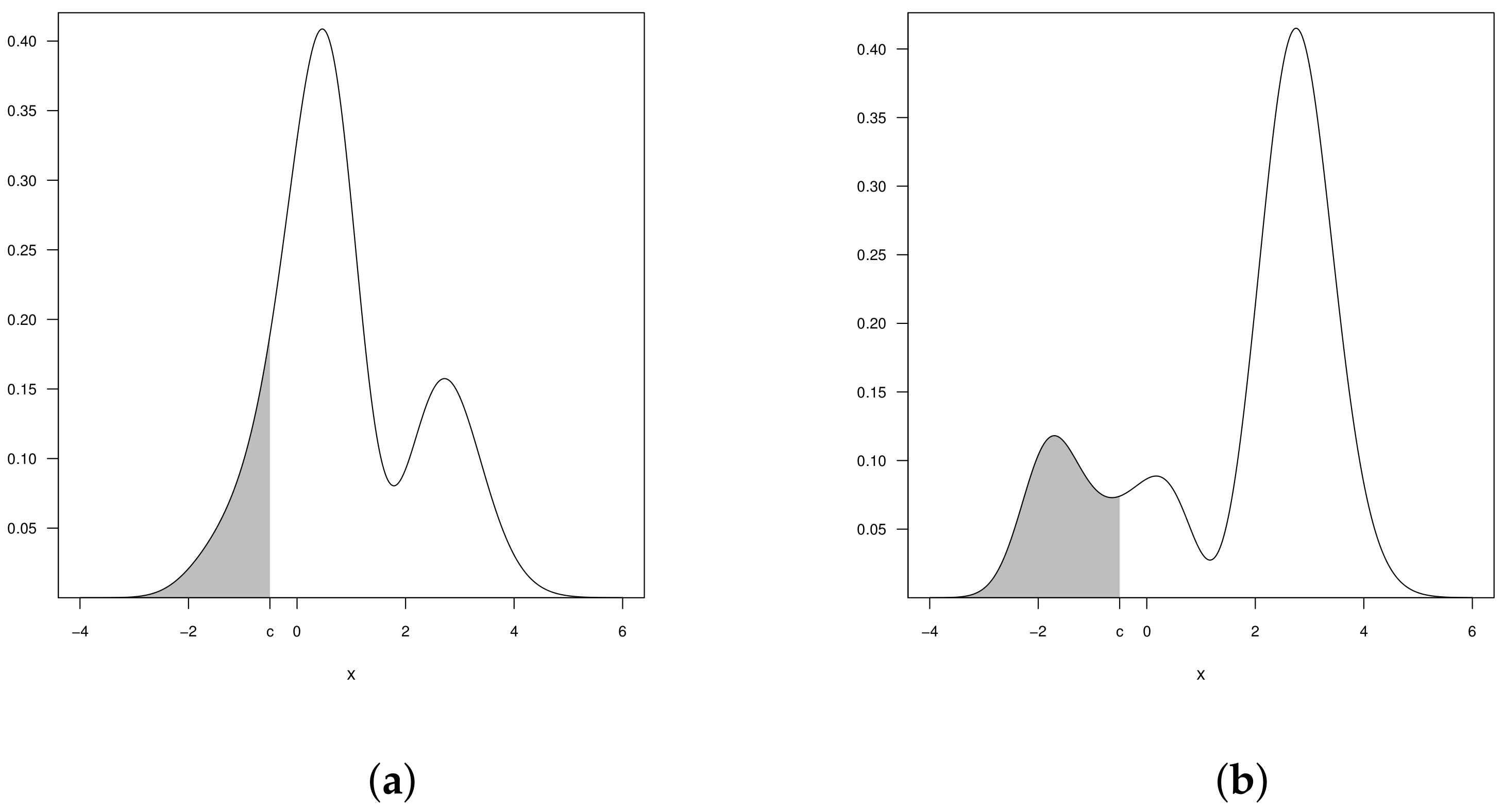
It can also see that, for
, it follows an asymmetric bimodal alpha-power model similar to CBSN model. Then, the CBSAP model can fit trimodal, bimodal or unimodal data set. The
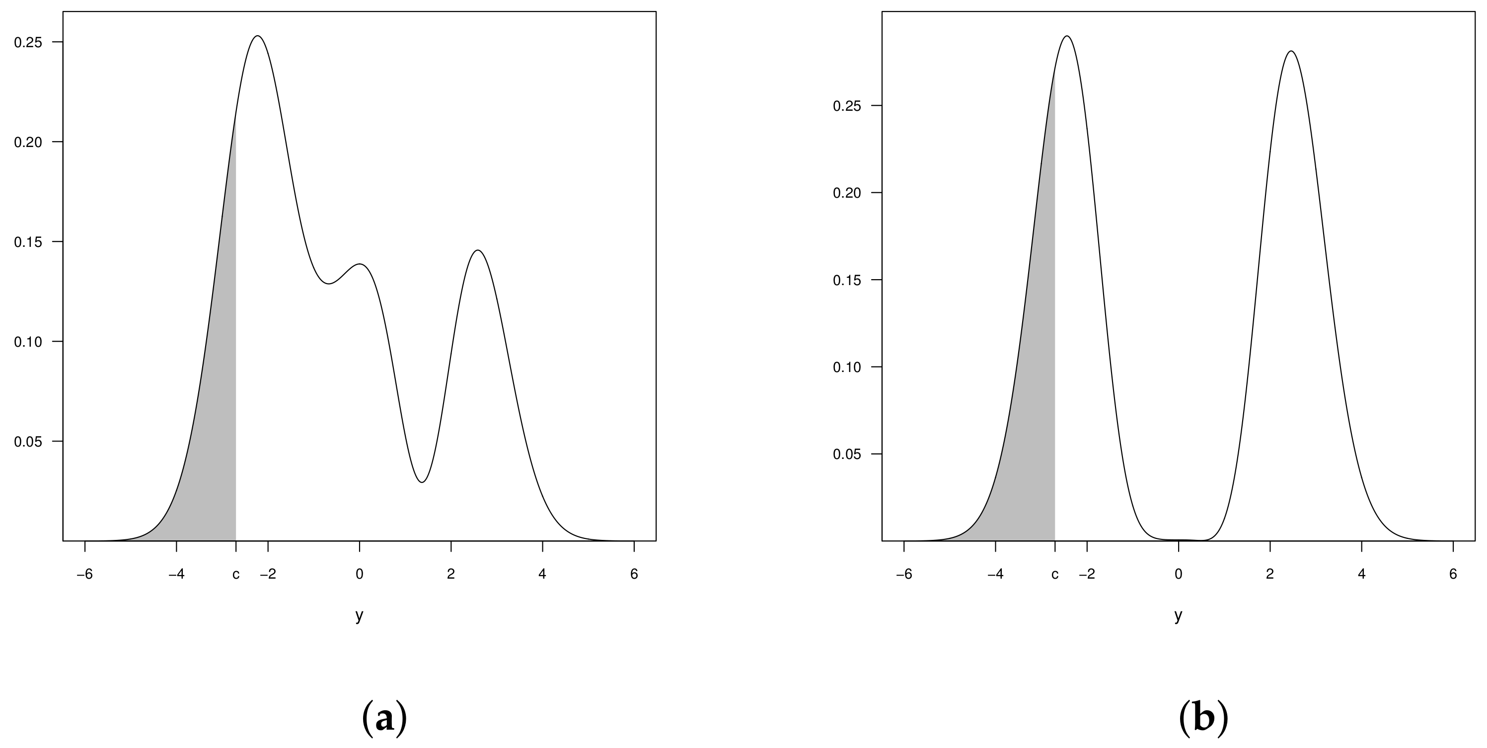
Figure 2 shows the graphs of the pdf of
with censorship point
, and for some values of the parameter
.
3.1. Inference for the CBSAP Model
This section discusses the parameters estimation of the vector
of the CBSAP distribution. In addition, the elements of the observed and expected information matrices are determined. Let
, a random sample of size
n from
with
, in which, there is
censored observations, and
uncensored observations. The likelihood function for
is given by
with
and
. The log-likelihood function obtained from (
20) is given by
Thus, by differentiating the log-likelihood function with respect to each of the parameters, the following score functions are obtained
By equating to zero the score functions (
21)–(
24) and solving the resulting system of equations, we obtain the maximum likelihood estimators (MLEs) of
,
,
and
, which can be obtained by numerical method such as the Newton–Raphson type procedure. Details about the theory of iterative methods to obtain the optimal solution to the system of equations can be found in Jäntschi et al. [
23].
The elements of the observed information matrix can be obtained by taking the second partial derivatives of the log-likelihood function and multiplying by −1, that is,
with
, and will be denoted by
. This elements are given in the
Appendix B.
Under certain regularity conditions, the elements of the Fisher information matrix can be calculated as
with
,
,
and
, and it will be denoted as
. The Cramér-Rao bound states that the inverse of the Fisher information is a lower bound on the variance of any unbiased estimator. Thus, we can find a lower bound for the standard errors (SE) of the MLEs as the root of the diagonal elements of the observed Fisher information matrix. The elements of the expected and observed Fisher information are given in the
Appendix B. For
y
the CBSAP model is reduced to the tobit model. In this case, following Martínez-Flórez et al. [
22] it can be seen that expected information matrix of the CBSAP model, say
is non-singular.
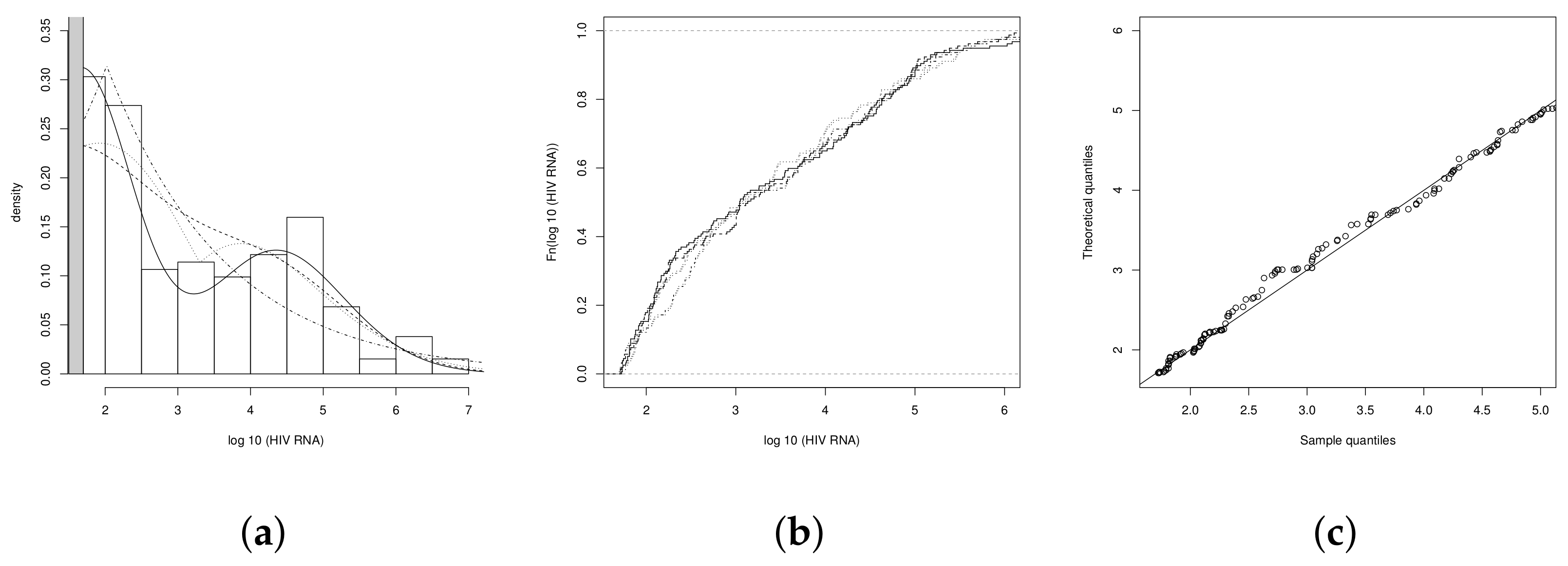
3.2. Model for Positive Data
Distributions with location and scale parameters for modeling positive data are not common in practice, among these, we find the log-normal model, log-skew-normal model by Azzalini et al. [
24] and log-power-normal model by Martínez-Flórez et al. [
25]. All these distributions, despite being very good tools to model this type of data, it can only be used in cases where the data distribution is unimodal, that is, they can not always be implemented in fields such as economics, health, engineering and many others, where the data present bimodality or multimodality. An initial proposal to model multimodal data is the mixture of unimodal distributions, for example, mixture of normals. However, many authors have developed new proposals that allow taking into account the asymmetry present in the data as well as their multimodality, see, for example, Elal-Olivero [
17], Bolfarine et al. [
10], Gómez et al. [
9], Shafiei et al. [
21].
We now present an extension of the beta-skew alpha-power model for modeling positive data, which is called the log-beta-skew alpha-power distribution and is denoted by LBSAP. This extension is introduced in the usual form of the location-scale models such as log-normal, log-skew-normal or log-power normal, that is, a random variable
X follows the LBSAP distribution if its logarithm follows the BSAP. Let
, where
and
are location and scale parameters, respectively, the pdf of
Y is given by
where
, with
and
. It follows that, the cdf for the location and scale version of
is given by the same expression of the cdf for the BSAP model with
. Occurs the same for the survival function, while, for the Hazard function, additionally it must be divided by
t, that is,
where
is the Hazard function of the
model with
.
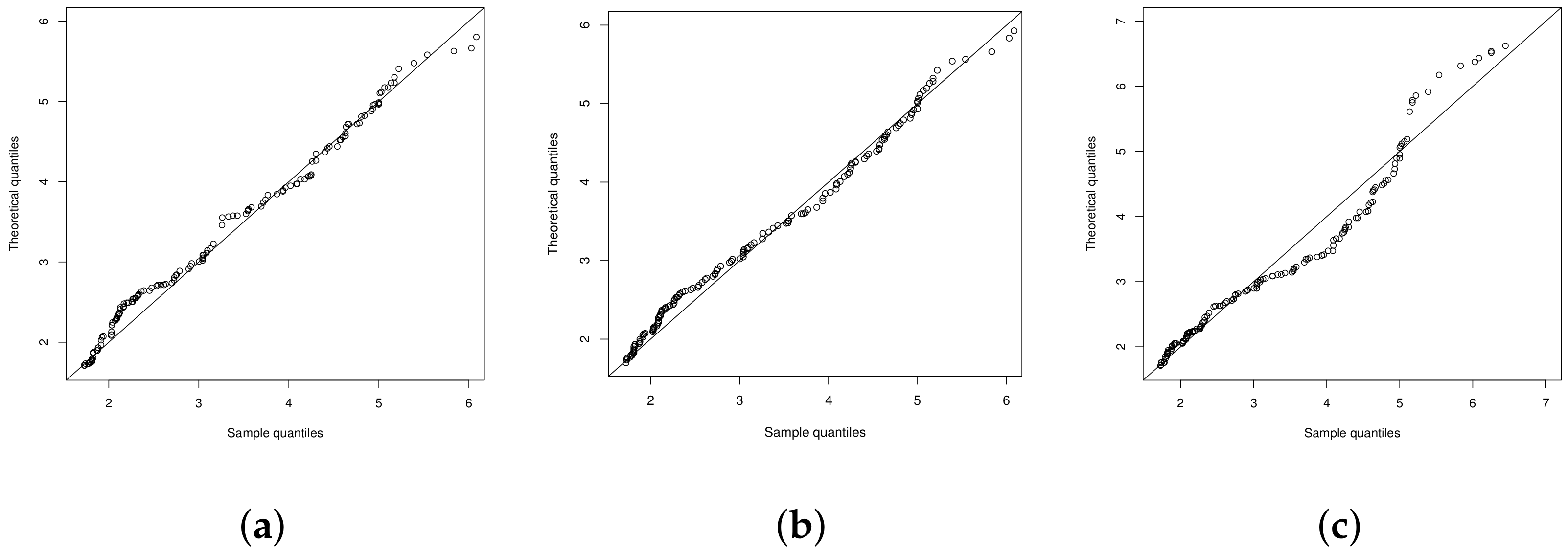
It follows that, if , the log-beta-skew-normal (LBSN) model is obtained, whereas, if and , then, it follows the log-normal model. From the properties that the BSAP model, it follows that the extension for positive data, that is, the LBSAP model can also fit data sets of up to three modes, even being bimodal or unimodal (case of the log-normal model). The moments of this distribution do not have a closed form and they are obtained directly from the definition by using numerical methods. The estimation of its parameters can be approached through the maximum likelihood method.
Let
a random sample of size
with
and
. Letting
for
, the log-likelihood function can be expressed as
Deriving the log-likelihood function with respect to each parameter and letting
, the following elements of the score function are obtained
The system of non-linear equations resulting from equating the first order derivatives to zero (score equations) does not have a closed solution, so it must be solved by using numerical methods. Thus, the maximum likelihood estimator for
can be obtained numerically via iterative algorithms such as, the Newton–Raphson or quasi-Newton. The elements of the observed and expected Fisher information matrix are obtained directly from the respective elements of the BSAP model, see Martínez-Flórez et al. [
22], by using
instead of
, hence, the matrix
of the
is non-singular. Thus, the covariances matrix of the estimators vector of the LBSAP distribution is given by
. Then, by the asymptotic convergence property of the maximum likelihood estimators, it follows
where
.
The study of the distribution for censored data is followed naturally from the results for the BSAP model. Suppose that
has a LBSAP distribution and we have a random sample
, where only the values greater than the constant
c are registered. Moreover, for values
, only the value of
c is recorded. Therefore, for
the observed values are written as
then, the result is a left-censored random sample LBSAP. The random variable
Y has pdf given by
where
is the pdf of a random variable with LBSAP distribution in the standard version, and
is the cdf of the Log BSN model. The model in (
32) is denoted by
, with
. Estimation for the parameters vector is carried out in a similar way as for the censored
model by Martínez-Flórez et al. [
22], where the score functions and the information matrices have the same structure and it is only necessary to change
instead of
and
instead of
.


