Tensor-Based Adaptive Filtering Algorithms

Abstract

Tensor-based signal processing methods are usually employed when dealing with multidimensional data and/or systems with a large parameter space. In this paper, we present a family of tensor-based adaptive filtering algorithms, which are suitable for high-dimension system identification problems. The basic idea is to exploit a decomposition-based approach, such that the global impulse response of the system can be estimated using a combination of shorter adaptive filters. The algorithms are mainly tailored for multiple-input/single-output system identification problems, where the input data and the channels can be grouped in the form of rank-1 tensors. Nevertheless, the approach could be further extended for single-input/single-output system identification scenarios, where the impulse responses (of more general forms) can be modeled as higher-rank tensors. As compared to the conventional adaptive filters, which involve a single (usually long) filter for the estimation of the global impulse response, the tensor-based algorithms achieve faster convergence rate and tracking, while also providing better accuracy of the solution. Simulation results support the theoretical findings and indicate the advantages of the tensor-based algorithms over the conventional ones, in terms of the main performance criteria.

1. Introduction

Nowadays, adaptive filtering algorithms represent powerful signal processing tools, which are widely used in many important applications [1]. Due to their capabilities to work in nonstationary environments and to process real-time data, these algorithms can provide efficient solutions for system identification problems [2], interference cancellation scenarios [3], and adaptive control processes [4].

In these frameworks, the least-mean-square (LMS) and the recursive least-squares (RLS) are the most popular categories of adaptive filtering algorithms [5]. The main advantage of the LMS-based algorithms consists of a lower computational complexity, as compared to their counterparts from the RLS family. Nevertheless, the latter ones are able to provide a faster convergence rate. On the other hand, the LMS algorithms are more sensitive to the character of the input data, e.g., when dealing with nonstationary or highly correlated inputs.

Currently, the interest for developing efficient algorithms for high-dimension system identification problems is increasing, while the solutions are mainly related to a tensorial approach and multilinear forms [6,7,8,9,10,11,12,13,14,15]. The gain of such methods is usually twofold, in terms of both performance and complexity. Linearly separable systems that are modeled based on the decomposition of rank-1 tensors can be exploited in the context of different applications. Among them, we can mention channel equalization [10,16], array beamforming [14,17], nonlinear acoustic echo cancellation [18,19], and source separation [11,20].

Basically, when dealing with a large parameter space, the system identification problem can be solved by using a decomposition into lower dimension structures, tensorized together. This kind of decomposition into two such smaller structures (i.e., bilinear forms) has been used before, and the initial system identification problem was addressed using different tools, such as an iterative version of the Wiener filter [21], adaptive algorithms [22,23], and the Kalman filter [24]. Furthermore, the trilinear forms are related to the decomposition of third-order tensors [8,15,25].

Recently, the iterative version of the Wiener filter was proposed for the identification of multilinear forms [26], aiming to provide a generalization of the previously developed solutions for bilinear/trilinear forms. In this way, the problem is addressed based on the decomposition of higher-order tensors, thus providing a general framework for efficiently solving high-dimension system identification problems. Nevertheless, the Wiener solution inherits some limitations, e.g., estimation of the statistics, matrix inversion operation, and stationarity assumption [5].

In this paper, we present a family of tensor-based adaptive filtering algorithms, which are able to overcome the previously mentioned limitations of the multilinear iterative Wiener filter. At this point, we are not centered on particular applications of these methods. The main goal of the current work is to provide a unified theoretical framework for developing such tensor-based algorithms that could be further developed in the context of specific applications. Moreover, the approach could be exploited beyond the identification of rank-1 tensors, aiming at efficient estimation methods for more general forms of long length impulse responses. It should be noted that such realistic impulse responses cannot be modeled as rank-1 tensors, but could own some specific characteristics that would facilitate an efficient tensor-based decomposition approach. For example, the sparseness character of the system could be considered, aiming to efficiently exploit the decomposition-based approach in conjunction with low-rank approximation methods. Therefore, the tensor-based algorithms presented in this paper could be further extended in this context.

The remainder of the paper is structured as follows. In Section 2, the system model is presented and the decomposition-based approach is introduced. The proposed algorithms are developed in Section 3 and Section 4, covering both the LMS and RLS families. A brief discussion concerning the identification of higher rank tensors is given in Section 5. Next, Section 6 provides extensive simulation results in the context of system identification. Finally, Section 7 outlines the conclusions and the main lines of our future works.

2. System Model

Let us consider a real-valued multiple-input/single-output (MISO) system, whose output at discrete-time index n can be written as

$$\begin{array}{cc}\hfill y\left(n\right)& =\sum _{l_1=1}^{L_1}\sum _{l_2=1}^{L_2}\cdots \sum _{l_N=1}^{L_N}{x}_{l_1{l}_2\dots l_N}\left(n\right)h_{1,l_1}{h}_{2,l_2}\cdots h_{N,l_N},\hfill \end{array}$$

(1)

with the N individual channels being characterized by the following vectors:

$$\begin{array}{cc}\hfill {\mathbf{h}}_i& ={\left[h_{i,1}{h}_{i,2}\cdots h_{i,L_i}\right]}^T,\hfill \end{array}$$

(2)

each one of length $L_i,i=1,2,\dots ,N$, where the superscript ${}^T$ is the transpose operator. We can group the input signals from (1) into a tensor $\mathcal{X}\left(n\right)\in {\mathbb{R}}^{L_1\times L_2\times \cdots \times L_N}$, with the elements ${\left(\mathcal{X}\right)}_{l_1{l}_2\dots l_N}\left(n\right)=x_{l_1{l}_2\dots l_N}\left(n\right)$. Hence, the output equation becomes

$$\begin{array}{cc}\hfill y\left(n\right)& =\mathcal{X}\left(n\right){\times }_1{\mathbf{h}}_1^T{\times }_2{\mathbf{h}}_2^T{\times }_3\cdots {\times }_N{\mathbf{h}}_N^T,\hfill \end{array}$$

(3)

where ${\times }_i,i=1,2,\dots ,N$ denotes the mode-i product [20]. In this way, $y\left(n\right)$ can be considered a multilinear form, because it represents a linear function of each of the vectors ${\mathbf{h}}_i,i=1,2,\dots ,N$, provided that the other $N-1$ vectors are kept fixed. Thus, it may be regarded as an extension of the bilinear form [21]. Next, we consider the tensor $\mathcal{H}\in {\mathbb{R}}^{L_1\times L_2\times \cdots \times L_N}$, with the elements ${\left(\mathcal{H}\right)}_{l_1,l_2,\dots ,l_N}=h_{1,l_1}{h}_{2,l_2}\cdots h_{N,l_N}$. This tensor can also be expressed as

$$\begin{array}{cc}\hfill \mathcal{H}& ={\mathbf{h}}_1\circ {\mathbf{h}}_2\circ \cdots \circ {\mathbf{h}}_N,\hfill \end{array}$$

(4)

where ∘ denotes the outer product. The outer product of two vectors is defined as ${\mathbf{h}}_1\circ {\mathbf{h}}_2={\mathbf{h}}_1{\mathbf{h}}_2^T$, with the elements ${\left({\mathbf{h}}_1\circ {\mathbf{h}}_2\right)}_{i,j}=h_{1,i}{h}_{2,j}$. The relation between the Kronecker product of two vectors and the corresponding outer product is ${\mathbf{h}}_2\otimes {\mathbf{h}}_1=\mathrm{vec}\left({\mathbf{h}}_1\circ {\mathbf{h}}_2\right)$. Furthermore, we have

$$\begin{array}{cc}\hfill \mathrm{vec}\left(\mathcal{H}\right)& ={\mathbf{h}}_N\otimes {\mathbf{h}}_{N-1}\otimes \cdots \otimes {\mathbf{h}}_1,\hfill \end{array}$$

(5)

where ⊗ represents the Kronecker product, whereas $\mathrm{vec}(·)$ denotes the vectorization operation, i.e.,

$$\begin{array}{cc}\hfill \mathrm{vec}\left(\mathcal{H}\right)& =\left[\begin{array}{c}\mathrm{vec}\left({\mathbf{H}}_{::\dots :1}\right)\\ \mathrm{vec}\left({\mathbf{H}}_{::\dots :2}\right)\\ ⋮\\ \mathrm{vec}\left({\mathbf{H}}_{::\dots :L_N}\right)\end{array}\right],\hfill \end{array}$$

(6)

$$\begin{array}{cc}\hfill \mathrm{vec}\left({\mathbf{H}}_{::\dots :l_i}\right)& =\left[\begin{array}{c}\mathrm{vec}\left({\mathbf{H}}_{::\dots :1,i}\right)\\ \mathrm{vec}\left({\mathbf{H}}_{::\dots :2,i}\right)\\ ⋮\\ \mathrm{vec}\left({\mathbf{H}}_{::\dots :L_{N-1,i}}\right)\end{array}\right],\hfill \end{array}$$

(7)

where ${\mathbf{H}}_{::\dots :l_i}\in {\mathbb{R}}^{L_1\times L_2\times \cdots \times L_{N-1}},i=1,2,\dots ,N$ are the frontal slices of $\mathcal{H}$. Consequently, the output signal can be re-written as

$$\begin{array}{cc}\hfill y\left(n\right)& ={\mathrm{vec}}^T\left(\mathcal{H}\right)\mathrm{vec}\left[\mathcal{X}\left(n\right)\right],\hfill \end{array}$$

(8)

with

$$\begin{array}{cc}\hfill \mathrm{vec}\left[\mathcal{X}\left(n\right)\right]& =\left[\begin{array}{c}\mathrm{vec}\left[{\mathbf{X}}_{::\dots :1}\left(n\right)\right]\\ \mathrm{vec}\left[{\mathbf{X}}_{::\dots :2}\left(n\right)\right]\\ ⋮\\ \mathrm{vec}\left[{\mathbf{X}}_{::\dots :L_N}\left(n\right)\right]\end{array}\right]=\mathbf{x}\left(n\right),\hfill \end{array}$$

(9)

where ${\mathbf{X}}_{::\dots :l_i}\left(n\right)\in {\mathbb{R}}^{L_1\times L_2\times \cdots \times L_{N-1}},i=1,2,\dots ,N$ are the frontal slices of $\mathcal{X}\left(n\right)$ and $\mathbf{x}\left(n\right)$ is the input vector of length $L_1{L}_2\cdots L_N$. Let us denote the global impulse response as

$$\begin{array}{cc}\hfill \mathbf{g}& =\mathrm{vec}\left(\mathcal{H}\right)={\mathbf{h}}_N\otimes {\mathbf{h}}_{N-1}\otimes \cdots \otimes {\mathbf{h}}_1,\hfill \end{array}$$

(10)

of length $L_1{L}_2\cdots L_N$. An important observation is that the decomposition in (10) does not yield a unique set of estimates of the individual components. For example, let us consider N real-valued constants $c_i$, with $i=1,2,\dots ,N$, such that ${\prod }_{i=1}^N{c}_i=1$. Therefore,

$$\begin{array}{cc}\hfill c_N{\mathbf{h}}_N\otimes c_{N-1}{\mathbf{h}}_{N-1}\otimes \cdots \otimes c_1{\mathbf{h}}_1& ={\mathbf{h}}_N\otimes {\mathbf{h}}_{N-1}\otimes \cdots \otimes {\mathbf{h}}_1.\hfill \end{array}$$

(11)

However, as we can notice, no scaling ambiguity appears from the identification of the global system $\mathbf{g}$.

Next, using (8)–(10), $y\left(n\right)$ can be expressed as

$$y\left(n\right)={\mathbf{g}}^T\mathbf{x}\left(n\right).$$

(12)

In this context, the goal is to identify the global impulse response $\mathbf{g}$ (or, equivalently, the individual components ${\mathbf{h}}_i,i=1,2,\dots ,N$), using the desired (or reference) signal:

$$\begin{array}{cc}\hfill d\left(n\right)& ={\mathbf{g}}^T\mathbf{x}\left(n\right)+w\left(n\right),\hfill \end{array}$$

(13)

where $w\left(n\right)$ represents the measurement noise, that is not correlated with the input signals. The desired signal’s variance is

$$\begin{array}{cc}\hfill {\sigma }_d^2& ={\mathbf{g}}^{T}E\left[\mathbf{x}\left(n\right){\mathbf{x}}^T\left(n\right)\right]\mathbf{g}+{\sigma }_w^2\hfill \\ \hfill & ={\mathbf{g}}^T\mathbf{R}\mathbf{g}+{\sigma }_w^2,\hfill \end{array}$$

(14)

where $E[·]$ denotes mathematical expectation, $\mathbf{R}=E\left[\mathbf{x}\left(n\right){\mathbf{x}}^T\left(n\right)\right]$, and ${\sigma }_w^2=E\left[w^2\left(n\right)\right]$.

At this moment, we can introduce the error signal:

$$\begin{array}{cc}\hfill e\left(n\right)& =d\left(n\right)-{\widehat{\mathbf{g}}}^T\mathbf{x}\left(n\right),\hfill \end{array}$$

(15)

where $\widehat{\mathbf{g}}$ is an estimate of the global impulse response. Using (15), the mean-squared error (MSE) criterion can be defined as

$$\begin{array}{cc}\hfill J\left(\widehat{\mathbf{g}}\right)& =E\left[e^2\left(n\right)\right]={\sigma }_d^2-2{\widehat{\mathbf{g}}}^T\mathbf{p}+{\widehat{\mathbf{g}}}^T\mathbf{R}\widehat{\mathbf{g}},\hfill \end{array}$$

(16)

where $\mathbf{p}=E\left[\mathbf{x}\left(n\right)d\left(n\right)\right]$ is the cross-correlation vector between $\mathbf{x}\left(n\right)$ and $d\left(n\right)$. Consequently, the purpose is the minimization of $J\left(\widehat{\mathbf{g}}\right)$, for which a very popular solution is provided by the Wiener filter [5]:

$$\begin{array}{cc}\hfill {\widehat{\mathbf{g}}}_{\mathrm{W}}& ={\mathbf{R}}^{-1}\mathbf{p}.\hfill \end{array}$$

(17)

In the context of multilinear forms, the iterative Wiener filter derived recently in [26] uses the global impulse response decomposition. The optimization criterion is applied using a block coordinate descent approach on the individual components [27]. As compared to the conventional Wiener solution from (17), the proposed iterative Wiener filter for multilinear forms yields a better performance, especially in the case when the estimation of the statistics (i.e., $\mathbf{R}$ and $\mathbf{p}$) is made using a small amount of data.

3. Tensor-Based LMS Algorithms

The matrix inversion and the statistics estimation needed when using the Wiener solutions presented before could be unsuitable in real-world scenarios (e.g., when dealing with nonstationary environments and/or requiring real-time processing). Consequently, it may be more practical to use adaptive filters, and among them, the LMS algorithm is one of the simplest and most practical solutions [7,28].

First, let us consider the estimated impulse responses of the channels, ${\widehat{\mathbf{h}}}_i\left(n\right)$, with $i=1,2,\dots ,N$. Therefore, we may define the corresponding a priori error signals:

$$\begin{array}{cc}\hfill e_{{\widehat{\mathbf{h}}}_i}\left(n\right)& =d\left(n\right)-{\widehat{\mathbf{h}}}_i^T(n-1){\mathbf{x}}_{{\widehat{\mathbf{h}}}_i}\left(n\right),\hfill \end{array}$$

(18)

with $i=1,2,\dots ,N$, where

$$\begin{array}{cc}\hfill {\mathbf{x}}_{{\widehat{\mathbf{h}}}_i}\left(n\right)& =\left[{\widehat{\mathbf{h}}}_N(n-1)\otimes {\widehat{\mathbf{h}}}_{N-1}(n-1)\otimes \cdots \otimes {\widehat{\mathbf{h}}}_{i+1}(n-1)\otimes {\mathbf{I}}_{L_i}\right.\hfill \\ \hfill & \otimes {\widehat{\mathbf{h}}}_{i-1}(n-1)\otimes {\left.\cdots \otimes {\widehat{\mathbf{h}}}_2(n-1)\otimes {\widehat{\mathbf{h}}}_1(n-1)\right]}^T\mathbf{x}\left(n\right),\hfill \end{array}$$

(19)

with ${\mathbf{I}}_{L_i},i=1,2,\dots ,N$ being the identity matrices of sizes $L_i\times L_i$. It is easy to check that $e_{{\widehat{\mathbf{h}}}_1}\left(n\right)=e_{{\widehat{\mathbf{h}}}_2}\left(n\right)=\cdots =e_{{\widehat{\mathbf{h}}}_N}\left(n\right)$. Consequently, the LMS updates of the individual filters result in

$$\begin{array}{cc}\hfill {\widehat{\mathbf{h}}}_i\left(n\right)& ={\widehat{\mathbf{h}}}_i(n-1)-\frac{{\mu }_i}{2}\times \frac{\partial e_{{\widehat{\mathbf{h}}}_i}^2\left(n\right)}{\partial {\widehat{\mathbf{h}}}_i(n-1)}\hfill \\ \hfill & ={\widehat{\mathbf{h}}}_i(n-1)+{\mu }_i{\mathbf{x}}_{{\widehat{\mathbf{h}}}_i}\left(n\right)e_{{\widehat{\mathbf{h}}}_i}\left(n\right),\hfill \end{array}$$

(20)

where ${\mu }_i>0,i=1,2,\dots ,N$ are the step-size parameters. Relations (20) define the tensor-based LMS (LMS-T) algorithm. The initialization of the algorithm could be

$$\begin{array}{cc}\hfill {\widehat{\mathbf{h}}}_1\left(0\right)& =\left[\begin{array}{c}1\hfill \\ {\mathbf{0}}_{L_1-1}\hfill \end{array}\right],\hfill \end{array}$$

(21)

$$\begin{array}{cc}\hfill {\widehat{\mathbf{h}}}_j\left(0\right)& =\frac{1}{L_j}{\mathbf{1}}_{L_j},j=2,3,\dots ,N,\hfill \end{array}$$

(22)

where ${\mathbf{0}}_P$ and ${\mathbf{1}}_P$ are two vectors of length P, whose all elements are equal to zero and one, respectively. We should also note that the classical “all-zeros” initialization used in most of the conventional adaptive filtering algorithms cannot be used in this case, due to the connection between the individual filters. In other words, using ${\widehat{\mathbf{h}}}_i\left(0\right)={\mathbf{0}}_{L_i},i=1,2,\dots ,N$ would “freeze” the updates (20) of the LMS-T algorithm, due to (19).

Finally, the estimate of the global system is obtained as

$$\begin{array}{cc}\hfill \widehat{\mathbf{g}}\left(n\right)& ={\widehat{\mathbf{h}}}_N\left(n\right)\otimes {\widehat{\mathbf{h}}}_{N-1}\left(n\right)\otimes \cdots \otimes {\widehat{\mathbf{h}}}_1\left(n\right).\hfill \end{array}$$

(23)

The global impulse response may also be identified using the conventional LMS algorithm [5]:

$$\begin{array}{cc}\hfill \widehat{\mathbf{g}}\left(n\right)& =\widehat{\mathbf{g}}(n-1)+\mu \mathbf{x}\left(n\right)e\left(n\right),\hfill \end{array}$$

(24)

$$\begin{array}{cc}\hfill e\left(n\right)& =d\left(n\right)-\widehat{\mathbf{g}}(n-1)\mathbf{x}\left(n\right),\hfill \end{array}$$

(25)

where $\mu$ is the global step-size parameter. According to (18), (19) and (23), it can be noticed that $e\left(n\right)=e_{{\widehat{\mathbf{h}}}_i}\left(n\right),i=1,2,\dots ,N$. However, the update (24) involves an adaptive filter of length $L={\prod }_{i=1}^N{L}_i$, while the LMS-T algorithm combines the solutions of N shorter filters of lengths $L_i$, with $i=1,2,\dots ,N$. Since the global performance of any adaptive algorithm is highly influenced by the length of the filter, the LMS-T algorithm should own improved features as compared to the conventional LMS counterpart. Simulation results provided in Section 6 support this aspect.

The convergence analysis of the LMS-T algorithm is not a straightforward task. The main challenge is related to the connection between the individual filters. According to (18)–(20), the coefficients of the i-th filter ($i=1,2,\dots ,N$) at time index n depend on the coefficients of the other $N-1$ individual filters from the previous time index ($n-1$). Based on the analogy with bilinear forms [7,22], the stability of the LMS-T algorithm is guaranteed for $0<{\mu }_i<2/{\sum }_{i=1}^N{\mathbf{x}}_{{\widehat{\mathbf{h}}}_i}^T\left(n\right){\mathbf{x}}_{{\widehat{\mathbf{h}}}_i}\left(n\right)$, assuming that ${\mu }_1={\mu }_2=\cdots ={\mu }_N$. This setup is also used by the tensor LMS algorithm proposed by Rupp and Schwarz in [7]. On the other hand, taking into account the well-known compromise between the convergence rate and misadjustment, this condition could be too restrictive if targeting different adaptation modes (i.e., different step-sizes) for the individual filters. Consequently, a detailed convergence analysis of the LMS-T algorithm is considered for future works.

Nevertheless, the selection of the step-sizes represents an important challenge when setting the parameters of the LMS-T algorithm. It can be noticed that, in (20), the step-size parameters are constant. A good compromise between convergence speed and misadjustment needs to be considered when choosing their values. Nevertheless, in nonstationary environments, it could be more useful to choose variable step-size (i.e., time-dependent) parameters. Consequently, the updates for the LMS algorithm should be reformulated as

$$\begin{array}{cc}\hfill {\widehat{\mathbf{h}}}_i\left(n\right)& ={\widehat{\mathbf{h}}}_i(n-1)+{\mu }_i\left(n\right){\mathbf{x}}_{{\widehat{\mathbf{h}}}_i}\left(n\right)e_{{\widehat{\mathbf{h}}}_i}\left(n\right),\hfill \end{array}$$

(26)

with $i=1,2,\dots ,N$. Next, we define the a posteriori error signals:

$$\begin{array}{cc}\hfill {\epsilon }_{{\widehat{\mathbf{h}}}_i}\left(n\right)& =d\left(n\right)-{\widehat{\mathbf{h}}}_i^T\left(n\right){\mathbf{x}}_{{\widehat{\mathbf{h}}}_i}\left(n\right),\hfill \end{array}$$

(27)

with $i=1,2,\dots ,N$. By replacing (20) in (27), then forcing the a posteriori error signals to zero, we obtain

$$\begin{array}{cc}\hfill e_{{\widehat{\mathbf{h}}}_i}\left(n\right)\left[1-{\mu }_i\left(n\right){\mathbf{x}}_{{\widehat{\mathbf{h}}}_i}^T\left(n\right){\mathbf{x}}_{{\widehat{\mathbf{h}}}_i}\left(n\right)\right]& =0,\hfill \end{array}$$

(28)

for $i=1,2,\dots ,N$. By assuming that $e_{{\widehat{\mathbf{h}}}_i}\left(n\right)\ne 0,i=1,2,\dots ,N$, the expressions of the time-dependent step-sizes result as

$$\begin{array}{cc}\hfill {\mu }_i\left(n\right)& =\frac{1}{{\mathbf{x}}_{{\widehat{\mathbf{h}}}_i}^T\left(n\right){\mathbf{x}}_{{\widehat{\mathbf{h}}}_i}\left(n\right)}.\hfill \end{array}$$

(29)

We also need to introduce some regularization constants ${\delta }_i>0,i=1,2,\dots ,N$ in the denominators of the above expressions [29], in order to achieve a robust adaptation. Moreover, in order to obtain a good compromise between convergence rate and steady-state misadjustment, the normalized step-size parameters $0<{\alpha }_i\le 1,i=1,2,\dots ,N$ are used. Hence, the update equations of the tensor-based normalized LMS (NLMS-T) algorithm are obtained as

$$\begin{array}{cc}\hfill {\widehat{\mathbf{h}}}_i\left(n\right)& ={\widehat{\mathbf{h}}}_i(n-1)+\frac{{\alpha }_i{\mathbf{x}}_{{\widehat{\mathbf{h}}}_i}\left(n\right)e_{{\widehat{\mathbf{h}}}_i}\left(n\right)}{{\delta }_i+{\mathbf{x}}_{{\widehat{\mathbf{h}}}_i}^T\left(n\right){\mathbf{x}}_{{\widehat{\mathbf{h}}}_i}\left(n\right)},\hfill \end{array}$$

(30)

with $i=1,2,\dots ,N$, while the global impulse response results similar to (23). Similarly, the individual impulse responses may be initialized using (21)–(22). The NLMS-T algorithm is summarized in Algorithm 1.

Algorithm 1: NLMS-T algorithm.

Initialization:       Set ${\widehat{\mathbf{h}}}_i\left(0\right),i=1,2,\dots ,N$, based on (21)–(22)       Set $0<{\alpha }_i\le 1,{\delta }_i>0,i=1,2,\dots ,N$       For n = 1,2,…, number of iterations:       Compute ${\mathbf{x}}_{{\widehat{\mathbf{h}}}_i}\left(n\right),i=1,2,\dots ,N$, based on (19)       $e_{{\widehat{\mathbf{h}}}_i}\left(n\right)=d\left(n\right)-{\widehat{\mathbf{h}}}_i^T(n-1){\mathbf{x}}_{{\widehat{\mathbf{h}}}_i}\left(n\right)$, for any $i=1,2,\dots ,N$       ${\widehat{\mathbf{h}}}_i\left(n\right)={\widehat{\mathbf{h}}}_i(n-1)+\frac{{\alpha }_i{\mathbf{x}}_{{\widehat{\mathbf{h}}}_i}\left(n\right)e_{{\widehat{\mathbf{h}}}_i}\left(n\right)}{{\delta }_i+{\mathbf{x}}_{{\widehat{\mathbf{h}}}_i}^T\left(n\right){\mathbf{x}}_{{\widehat{\mathbf{h}}}_i}\left(n\right)},i=1,2,\dots ,N$       $\widehat{\mathbf{g}}\left(n\right)={\widehat{\mathbf{h}}}_N\left(n\right)\otimes {\widehat{\mathbf{h}}}_{N-1}\left(n\right)\otimes \cdots \otimes {\widehat{\mathbf{h}}}_1\left(n\right)$

Another way to identify the global impulse response is to use the conventional normalized LMS (NLMS) algorithm [5], defined by

$$\begin{array}{cc}\hfill \widehat{\mathbf{g}}\left(n\right)& =\widehat{\mathbf{g}}(n-1)+\frac{\alpha \mathbf{x}\left(n\right)e\left(n\right)}{\delta +{\mathbf{x}}^T\left(n\right)\mathbf{x}\left(n\right)},\hfill \end{array}$$

(31)

where $0<\alpha \le 1$ denotes the normalized step-size parameter, $\delta >0$ is the regularization constant, and $e\left(n\right)$ was defined in (25). Nevertheless, similar to the previous discussion related to the LMS-T and LMS algorithms, the NLMS-T uses N adaptive filters of lengths $L_i,i=1,2,\dots ,N$, while the length of the conventional NLMS filter is $L={\prod }_{i=1}^N{L}_i$.

4. Tensor-Based RLS Algorithm

The main advantage of the RLS-based algorithms consists of a faster convergence rate, as compared to the LMS family. This gain is more apparent for correlated input signals. On the other hand, the price to pay is a higher computational complexity. In this context, the tensor-based algorithms could be more advantageous. In the following, we exploit this approach in the case of the RLS algorithm.

Let us consider the context of (13) and (15), where we apply the least-squares error criterion [5]. As a result, the conventional RLS algorithm can be derived following the minimization of the cost function:

$$\begin{array}{cc}\hfill J\left[\widehat{\mathbf{g}}\left(n\right)\right]& =\sum _{k=1}^n{\lambda }^{n-k}{\left[d\left(k\right)-{\widehat{\mathbf{g}}}^T\left(n\right)\mathbf{x}\left(k\right)\right]}^2,\hfill \end{array}$$

(32)

where $0<\lambda \le 1$ is the forgetting factor of the algorithm. Equivalently, using (19), the cost function (32) can be reformulated in N alternative ways, following the optimization procedure of the individual impulse responses, i.e.,

$$\begin{array}{cc}\hfill J_{{\widehat{\mathbf{h}}}_N,{\widehat{\mathbf{h}}}_{N-1},\dots ,{\widehat{\mathbf{h}}}_{i+1},{\widehat{\mathbf{h}}}_{i-1},\dots ,{\widehat{\mathbf{h}}}_2,{\widehat{\mathbf{h}}}_1}\left[{\widehat{\mathbf{h}}}_i\left(n\right)\right]& =\sum _{k=1}^n{\lambda }_i^{n-k}{\left[d\left(k\right)-{\widehat{\mathbf{h}}}_i^T\left(n\right){\mathbf{x}}_{{\widehat{\mathbf{h}}}_i}\left(k\right)\right]}^2,\hfill \end{array}$$

(33)

with $i=1,2,\dots ,N$, where the ${\lambda }_i$’s are the individual forgetting factors. These cost functions are further processed following a multilinear optimization strategy [27]. In other words, we consider that $N-1$ components are fixed, while the optimization procedure is related to the remaining one. Therefore, following the minimization of (33) with respect to ${\widehat{\mathbf{h}}}_i\left(n\right)$, for $i=1,2,\dots ,N$, we obtain a set of normal equations:

$$\begin{array}{cc}\hfill {\mathbf{R}}_i\left(n\right){\widehat{\mathbf{h}}}_i\left(n\right)& ={\mathbf{p}}_i\left(n\right),\hfill \end{array}$$

(34)

where

$$\begin{array}{cc}\hfill {\mathbf{R}}_i\left(n\right)& =\sum _{k=1}^n{\lambda }_i^{n-k}{\mathbf{x}}_{{\widehat{\mathbf{h}}}_i}\left(k\right){\mathbf{x}}_{{\widehat{\mathbf{h}}}_i}^T\left(k\right)\hfill \end{array}$$

$$\begin{array}{cc}\hfill & ={\lambda }_i{\mathbf{R}}_i(n-1)+{\mathbf{x}}_{{\widehat{\mathbf{h}}}_i}\left(n\right){\mathbf{x}}_{{\widehat{\mathbf{h}}}_i}^T\left(n\right),\hfill \\ \hfill {\mathbf{p}}_i\left(n\right)& =\sum _{k=1}^n{\lambda }_i^{n-k}{\mathbf{x}}_{{\widehat{\mathbf{h}}}_i}\left(k\right)d\left(k\right)\hfill \end{array}$$

(35)

$$\begin{array}{cc}\hfill & ={\lambda }_i{\mathbf{p}}_i(n-1)+{\mathbf{x}}_{{\widehat{\mathbf{h}}}_i}\left(n\right)d\left(n\right),\hfill \end{array}$$

(36)

with $i=1,2,\dots ,N$. Solving (34), we obtain N update relations related to the individual filters, which result in

$$\begin{array}{cc}\hfill {\widehat{\mathbf{h}}}_i\left(n\right)& ={\widehat{\mathbf{h}}}_i(n-1)+{\mathbf{R}}_i^{-1}\left(n\right){\mathbf{x}}_{{\widehat{\mathbf{h}}}_i}\left(n\right)e_{{\widehat{\mathbf{h}}}_i}\left(n\right)\hfill \\ \hfill & ={\widehat{\mathbf{h}}}_i(n-1)+{\mathbf{k}}_i\left(n\right)e_{{\widehat{\mathbf{h}}}_i}\left(n\right),\hfill \end{array}$$

(37)

for $i=1,2,\dots ,N$, where ${\mathbf{k}}_i\left(n\right)={\mathbf{R}}_i^{-1}\left(n\right){\mathbf{x}}_{{\widehat{\mathbf{h}}}_i}\left(n\right)$ are the Kalman gain vectors. Furthermore, we can use (18) to compute the error signal.

An important issue is related to the inverse of the matrices ${\mathbf{R}}_i\left(n\right),i=1,2,\dots ,N$. This can be efficiently addressed based on the matrix inversion lemma, which is also known as the Woodbury matrix identity [5]. This states that having the matrices $\mathbf{A}$, $\mathbf{B}$, $\mathbf{C}$, $\mathbf{D}$, and $\mathbf{E}$ (with consistent sizes), such that $\mathbf{A}=\mathbf{B}+\mathbf{C}\mathbf{D}\mathbf{E}$, the inverse of this matrix results in ${\mathbf{A}}^{-1}={\mathbf{B}}^{-1}-{\mathbf{B}}^{-1}\mathbf{C}{\left({\mathbf{D}}^{-1}+\mathbf{E}\mathbf{B}{\mathbf{C}}^{-1}\right)}^{-1}\mathbf{E}{\mathbf{B}}^{-1}$. Consequently, in (35), we can associate $\mathbf{A}={\mathbf{R}}_i\left(n\right)$, $\mathbf{B}={\lambda }_i{\mathbf{R}}_i(n-1)$, $\mathbf{C}={\mathbf{x}}_{{\widehat{\mathbf{h}}}_i}\left(n\right)$, $\mathbf{D}=1$, and $\mathbf{E}={\mathbf{x}}_{{\widehat{\mathbf{h}}}_i}^T\left(n\right)$, thus resulting the following updates:

$$\begin{array}{cc}\hfill {\mathbf{R}}_i^{-1}\left(n\right)& =\frac{1}{{\lambda }_i}\left[{\mathbf{I}}_{L_i}-{\mathbf{k}}_i\left(n\right){\mathbf{x}}_{{\widehat{\mathbf{h}}}_i}^T\left(n\right)\right]{\mathbf{R}}_i^{-1}(n-1),\hfill \end{array}$$

(38)

with $i=1,2,\dots ,N$. The stability of such an update is guaranteed if the matrix ${\mathbf{R}}_i(n-1)$ is nonsingular and $0<{\lambda }_i\le 1,i=1,2,\dots ,N$. Consequently, the initialization should be ${\mathbf{R}}_i^{-1}\left(0\right)={\xi }_i^{-1}{\mathbf{I}}_{L_i},i=1,2,\dots ,N$, where ${\xi }_i$ is a positive constant.

Furthermore, the evaluation of the Kalman gain vectors results in

$$\begin{array}{cc}\hfill {\mathbf{k}}_i\left(n\right)& =\frac{{\mathbf{R}}_i^{-1}(n-1){\mathbf{x}}_{{\widehat{\mathbf{h}}}_i}\left(n\right)}{{\lambda }_i+{\mathbf{x}}_{{\widehat{\mathbf{h}}}_i}^T\left(n\right){\mathbf{R}}_i^{-1}(n-1){\mathbf{x}}_{{\widehat{\mathbf{h}}}_i}\left(n\right)},\hfill \end{array}$$

(39)

for $i=1,2,\dots ,N$. For initialization, we can follow the same rule from (21)–(22), while the global impulse response is obtained using (23). The resulting tensor-based RLS (RLS-T) algorithm is provided in Algorithm 2.

Algorithm 2: RLS-T algorithm.

Initialization:       Set ${\widehat{\mathbf{h}}}_i\left(0\right),i=1,2,\dots ,N$, based on (21)–(22)       ${\mathbf{R}}_i^{-1}\left(0\right)={\xi }_i^{-1}{\mathbf{I}}_{L_i},{\xi }_i>0,i=1,2,\dots ,N$       ${\lambda }_i=1-\frac{1}{K{L}_i},K\ge 1,i=1,2,\dots ,N$       For n = 1, 2,…, number of iterations:       Compute ${\mathbf{x}}_{{\widehat{\mathbf{h}}}_i}\left(n\right),i=1,2,\dots ,N$, based on (19)       $e_{{\widehat{\mathbf{h}}}_i}\left(n\right)=d\left(n\right)-{\widehat{\mathbf{h}}}_i^T(n-1){\mathbf{x}}_{{\widehat{\mathbf{h}}}_i}\left(n\right)$, for any $i=1,2,\dots ,N$       ${\mathbf{k}}_i\left(n\right)=\frac{{\mathbf{R}}_i^{-1}(n-1){\mathbf{x}}_{{\widehat{\mathbf{h}}}_i}\left(n\right)}{{\lambda }_i+{\mathbf{x}}_{{\widehat{\mathbf{h}}}_i}^T\left(n\right){\mathbf{R}}_i^{-1}(n-1){\mathbf{x}}_{{\widehat{\mathbf{h}}}_i}\left(n\right)},i=1,2,\dots ,N$       ${\widehat{\mathbf{h}}}_i\left(n\right)={\widehat{\mathbf{h}}}_i(n-1)+{\mathbf{k}}_i\left(n\right)e_{{\widehat{\mathbf{h}}}_i}\left(n\right),i=1,2,\dots ,N$       ${\mathbf{R}}_i^{-1}\left(n\right)=\frac{1}{{\lambda }_i}\left[{\mathbf{I}}_{L_i}-{\mathbf{k}}_i\left(n\right){\mathbf{x}}_{{\widehat{\mathbf{h}}}_i}^T\left(n\right)\right]{\mathbf{R}}_i^{-1}(n-1),i=1,2,\dots ,N$       $\widehat{\mathbf{g}}\left(n\right)={\widehat{\mathbf{h}}}_N\left(n\right)\otimes {\widehat{\mathbf{h}}}_{N-1}\left(n\right)\otimes \cdots \otimes {\widehat{\mathbf{h}}}_1\left(n\right)$

The convergence of the RLS-T algorithm can be assessed in terms of its conversion factors [5], based on the evaluation of the a posteriori errors. Using the update (37) in (27) and taking (15) into account, we obtain

$$\begin{array}{cc}\hfill {\epsilon }_{{\widehat{\mathbf{h}}}_i}\left(n\right)& =\left[1-{\mathbf{k}}_i^T\left(t\right){\mathbf{x}}_{{\widehat{\mathbf{h}}}_i}\left(n\right)\right]e_{{\widehat{\mathbf{h}}}_i}\left(n\right)\hfill \\ \hfill & ={\gamma }_i\left(n\right)e_{{\widehat{\mathbf{h}}}_i}\left(n\right),\hfill \end{array}$$

(40)

where ${\gamma }_i\left(n\right)=1-{\mathbf{k}}_i^T\left(t\right){\mathbf{x}}_{{\widehat{\mathbf{h}}}_i}\left(n\right),i=1,2,\dots ,N$ are the conversion factors. Next, replacing (39) into the expressions of the corresponding conversion factors, we obtain

$$\begin{array}{c}\hfill {\gamma }_i\left(n\right)=\frac{1}{1+{\lambda }_i^{-1}{\mathbf{x}}_{{\widehat{\mathbf{h}}}_i}^T\left(n\right){\mathbf{R}}_i^{-1}(n-1){\mathbf{x}}_{{\widehat{\mathbf{h}}}_i}\left(n\right)},\end{array}$$

(41)

for $i=1,2,\dots ,N$. Since ${\mathbf{R}}_i^{-1}(n-1)$ is a positive-definite matrix, we have ${\mathbf{x}}_{{\widehat{\mathbf{h}}}_i}^T\left(n\right){\mathbf{R}}_i^{-1}(n-1){\mathbf{x}}_{{\widehat{\mathbf{h}}}_i}\left(n\right)\ge 0$. Consequently, $0<{\gamma }_i\left(n\right)\le 1$, so that $|{\epsilon }_{{\widehat{\mathbf{h}}}_i}\left(n\right)|\le |e_{{\widehat{\mathbf{h}}}_i}\left(n\right)|$, for any $i=1,2,\dots ,N$. Therefore, the RLS-T algorithm is convergent.

Using the conventional RLS algorithm [5] for the estimation of the global impulse response could be prohibitive for large values of L, since the computational complexity order would be $\mathcal{O}\left(L^2\right)$. On the other hand, the computational complexity of the RLS-T algorithm is proportional to ${\sum }_{i=1}^N\mathcal{O}\left(L_i^2\right)$, which could be much more advantageous when $L_i\ll L$. In addition, since the RLS-T operates with shorter filters, improved performance is expected, as compared to the conventional RLS algorithm. This is also supported by the simulation results provided in Section 6.

5. Beyond the Identification of Rank-1 Tensors

The tensor-based algorithms developed in Section 3 and Section 4 are designed based the model presented in Section 2, so that they are suitable for the identification of rank-1 tensors. The optimization approach can be formulated in terms of the minimization of the system misalignment, which can be defined as

$$\begin{array}{cc}\hfill \mathcal{M}\left(\mathcal{H}\right)& =\frac{\parallel \mathcal{H}-{\widehat{\mathbf{h}}}_1\left(n\right)\circ {\widehat{\mathbf{h}}}_2\left(n\right)\circ \cdots \circ {\widehat{\mathbf{h}}}_N{\left(n\right)\parallel }_{\mathrm{F}}}{{\parallel \mathcal{H}\parallel }_{\mathrm{F}}},\hfill \end{array}$$

(42)

where ${\parallel ·\parallel }_{\mathrm{F}}$ denotes the Frobenius norm and $\mathcal{H}$ is defined in (4). Alternatively, (42) can also be expressed as

$$\begin{array}{cc}\hfill \mathcal{M}\left(\mathbf{g}\right)& =\frac{\parallel \mathbf{g}-{\widehat{\mathbf{h}}}_N\left(n\right)\otimes \cdots \otimes {\widehat{\mathbf{h}}}_2\left(n\right)\otimes {\widehat{\mathbf{h}}}_1{\left(n\right)\parallel }_2}{{\parallel \mathbf{g}\parallel }_2},\hfill \end{array}$$

(43)

where ${∥·∥}_2$ is the ${\ell }_2$ norm and $\mathbf{g}$ is given in (10).

As we can notice in (4), $\mathcal{H}$ is a rank-1 tensor [20], so that its individual components ${\mathbf{h}}_i,i=1,2,\dots ,N$ form the global impulse response $\mathbf{g}$ from (10), which represents a perfectly separable system. This repetitive (but not periodic) structure can result if a certain impulse response is followed by its reflections, e.g., as in wireless transmissions [7]. In addition, an external noise could also corrupt such impulse responses. However, even in this case, the tensor-based adaptive algorithms can efficiently model the separable part of the system, as will be shown in the last set of experiments reported in Section 6.

Nevertheless, the next goal is to extend the ideas behind the tensor-based algorithms for the identification of more general forms of impulse responses. This problem can be formulated in terms of identifying a higher rank tensor. It is known that the rank (R) of a tensor ${\mathcal{H}}_R$ is defined as the minimum number of rank-1 tensors that generate ${\mathcal{H}}_R$ as their sum, i.e.,

$$\begin{array}{cc}\hfill {\mathcal{H}}_R& =\sum _{r=1}^R{\mathbf{h}}_{1,r}\circ {\mathbf{h}}_{2,r}\circ \cdots \circ {\mathbf{h}}_{N,r},\hfill \end{array}$$

(44)

which represents the canonical polyadic decomposition (CPD) of the tensor [20]. Consequently, the optimization problem can be reformulated in terms of minimizing

$$\begin{array}{cc}\hfill \mathcal{M}\left({\mathcal{H}}_R\right)& =\frac{\parallel {\mathcal{H}}_R-{\sum }_{r=1}^R{\widehat{\mathbf{h}}}_{1,r}\left(n\right)\circ {\widehat{\mathbf{h}}}_{2,r}\left(n\right)\circ \cdots \circ {\widehat{\mathbf{h}}}_{N,r}{\left(n\right)\parallel }_{\mathrm{F}}}{\parallel {\mathcal{H}}_R{\parallel }_{\mathrm{F}}}\hfill \end{array}$$

(45)

or, alternatively,

$$\begin{array}{cc}\hfill \mathcal{M}\left(\underline{\mathbf{h}}\right)& =\frac{\parallel \underline{\mathbf{h}}-{\sum }_{r=1}^R{\widehat{\mathbf{h}}}_{N,r}\left(n\right)\otimes \cdots \otimes {\widehat{\mathbf{h}}}_{2,r}\left(n\right)\otimes {\widehat{\mathbf{h}}}_{1,r}{\left(n\right)\parallel }_2}{\parallel \underline{\mathbf{h}}{\parallel }_2},\hfill \end{array}$$

(46)

where ${\widehat{\mathbf{h}}}_{i,r}\left(n\right)$ represents the estimate of ${\mathbf{h}}_{i,r},i=1,2,\dots ,N$ and $\underline{\mathbf{h}}=\mathrm{vec}\left({\mathcal{H}}_R\right)={\sum }_{r=1}^R{\mathbf{h}}_{N,r}\otimes \cdots \otimes {\mathbf{h}}_{2,r}\otimes {\mathbf{h}}_{1,r}$.

Furthermore, in many real-world applications, we could exploit low-rank approximation methods in conjunction with tensor-based decompositions. In other words, we can use the approximation:

$$\begin{array}{c}\hfill \underline{\mathbf{h}}\approx \sum _{r=1}^P{\mathbf{h}}_{N,r}\otimes \cdots \otimes {\mathbf{h}}_{2,r}\otimes {\mathbf{h}}_{1,r},\end{array}$$

(47)

with $P<R$, so that an estimate of the impulse response can be obtained as

$$\begin{array}{c}\hfill \underline{\widehat{\mathbf{h}}}\left(n\right)=\sum _{r=1}^P{\widehat{\mathbf{h}}}_{N,r}\left(n\right)\otimes \cdots \otimes {\widehat{\mathbf{h}}}_{2,r}\left(n\right)\otimes {\widehat{\mathbf{h}}}_{1,r}\left(n\right).\end{array}$$

(48)

In our recent works [30,31], we approached these ideas in the two-dimensional case (i.e., $N=2$), by exploiting the singular value decomposition (SVD) of the system matrix (i.e., a second-order tensor). The framework was the echo cancellation problem, where the low-rank approximation fits very well, since the system matrix is never really full rank (due to the reflections and sparseness in the system).

For example, let us consider a single-input/single-output (SISO) system identification problem, where the reference signal is obtained as

$$\begin{array}{cc}\hfill \underline{d}\left(n\right)& ={\underline{\mathbf{h}}}^T\underline{\mathbf{x}}\left(n\right)+w\left(n\right),\hfill \end{array}$$

(49)

where $\underline{\mathbf{h}}$ (of length $\underline{L}$) is the unknown impulse response, $\underline{\mathbf{x}}\left(n\right)$ contains the most recent $\underline{L}$ time samples of the zero-mean input signal, and $w\left(n\right)$ is the additive noise (similar to (13)). In addition, we consider that $\underline{L}={\underline{L}}_1{\underline{L}}_2$, with ${\underline{L}}_1\ge {\underline{L}}_2$, so that the impulse response can be decomposed as

$$\begin{array}{cc}\hfill \underline{\mathbf{h}}& ={\left[\begin{array}{cccc}{\mathbf{s}}_1^T& {\mathbf{s}}_2^T& \cdots & {\mathbf{s}}_{{\underline{L}}_2}^T\end{array}\right]}^T,\hfill \end{array}$$

(50)

where ${\mathbf{s}}_l,l=1,2,\dots ,{\underline{L}}_2$ are ${\underline{L}}_2$ impulse responses, each of them having the length ${\underline{L}}_1$. Furthermore, the impulse response could be reshaped in a matrix form (of size ${\underline{L}}_1\times {\underline{L}}_2$), i.e.,

$$\begin{array}{cc}\hfill \underline{\mathbf{H}}& =\left[\begin{array}{cccc}{\mathbf{s}}_1& {\mathbf{s}}_2& \cdots & {\mathbf{s}}_{{\underline{L}}_2}\end{array}\right].\hfill \end{array}$$

(51)

As outlined before, if the rank of this matrix is $\mathrm{rank}\left(\underline{\mathbf{H}}\right)=P<{\underline{L}}_2$, the impulse response $\underline{\mathbf{h}}$ can be decomposed as

$$\begin{array}{cc}\hfill \underline{\mathbf{h}}& =\sum _{p=1}^P{\mathbf{h}}_{2,p}\otimes {\mathbf{h}}_{1,p},\hfill \end{array}$$

(52)

where ${\mathbf{h}}_{1,p}$ and ${\mathbf{h}}_{2,p}$ (with $p=1,2,\dots ,P$) are impulse responses of lengths ${\underline{L}}_1$ and ${\underline{L}}_2$, respectively.

Consequently, the impulse response of the adaptive filter could also be decomposed as

$$\begin{array}{cc}\hfill \underline{\widehat{\mathbf{h}}}\left(n\right)& =\sum _{p=1}^P{\widehat{\mathbf{h}}}_{2,p}\left(n\right)\otimes {\widehat{\mathbf{h}}}_{1,p}\left(n\right),\hfill \end{array}$$

(53)

where ${\widehat{\mathbf{h}}}_{1,p}\left(n\right)$ and ${\widehat{\mathbf{h}}}_{2,p}\left(n\right)$ have the lengths ${\underline{L}}_1$ and ${\underline{L}}_2$, respectively, while the error signal is evaluated as

$$\begin{array}{cc}\hfill \underline{e}\left(n\right)& =\underline{d}\left(n\right)-{\underline{\widehat{\mathbf{h}}}}^T(n-1)\underline{\mathbf{x}}\left(n\right).\hfill \end{array}$$

(54)

Following the least-squares error criterion [5] and taking (53) and (54) into account, the cost functions can be defined as

$$\begin{array}{cc}\hfill J_{{\underline{\widehat{\mathbf{h}}}}_2}\left[{\underline{\widehat{\mathbf{h}}}}_1\left(n\right)\right]& =\sum _{k=1}^n{\underline{\lambda }}_1^{n-k}{\left[\underline{d}\left(k\right)-{\underline{\widehat{\mathbf{h}}}}_1^T\left(n\right){\underline{\mathbf{x}}}_2\left(k\right)\right]}^2,\hfill \end{array}$$

(55)

$$\begin{array}{cc}\hfill J_{{\underline{\widehat{\mathbf{h}}}}_1}\left[{\underline{\widehat{\mathbf{h}}}}_2\left(n\right)\right]& =\sum _{k=1}^n{\underline{\lambda }}_2^{n-k}{\left[\underline{d}\left(k\right)-{\underline{\widehat{\mathbf{h}}}}_2^T\left(n\right){\underline{\mathbf{x}}}_1\left(k\right)\right]}^2,\hfill \end{array}$$

(56)

where ${\underline{\lambda }}_1$ and ${\underline{\lambda }}_2$ represent the forgetting factors, and

$$\begin{array}{cc}\hfill {\underline{\widehat{\mathbf{h}}}}_1\left(n\right)& ={\left[\begin{array}{cccc}{\widehat{\mathbf{h}}}_{1,1}^T\left(n\right)& {\widehat{\mathbf{h}}}_{1,2}^T\left(n\right)& \cdots & {\widehat{\mathbf{h}}}_{1,P}^T\left(n\right)\end{array}\right]}^T,\hfill \\ \hfill {\underline{\mathbf{x}}}_2\left(n\right)& ={\left[\begin{array}{cccc}{\mathbf{x}}_{2,1}^T\left(n\right)& {\mathbf{x}}_{2,2}^T\left(n\right)& \cdots & {\mathbf{x}}_{2,P}^T\left(n\right)\end{array}\right]}^T,\hfill \\ \hfill {\mathbf{x}}_{2,p}\left(n\right)& ={\left[{\widehat{\mathbf{h}}}_{2,p}(n-1)\otimes {\mathbf{I}}_{{\underline{L}}_1}\right]}^T\underline{\mathbf{x}}\left(n\right),p=1,2,\dots ,P,\hfill \\ \hfill {\underline{\widehat{\mathbf{h}}}}_2\left(n\right)& ={\left[\begin{array}{cccc}{\widehat{\mathbf{h}}}_{2,1}^T\left(n\right)& {\widehat{\mathbf{h}}}_{2,2}^T\left(n\right)& \cdots & {\widehat{\mathbf{h}}}_{2,P}^T\left(n\right)\end{array}\right]}^T,\hfill \\ \hfill {\underline{\mathbf{x}}}_1\left(n\right)& ={\left[\begin{array}{cccc}{\mathbf{x}}_{1,1}^T\left(n\right)& {\mathbf{x}}_{1,2}^T\left(n\right)& \cdots & {\mathbf{x}}_{1,P}^T\left(n\right)\end{array}\right]}^T,\hfill \\ \hfill {\mathbf{x}}_{1,p}\left(n\right)& ={\left[{\mathbf{I}}_{{\underline{L}}_2}\otimes {\widehat{\mathbf{h}}}_{1,p}(n-1)\right]}^T\underline{\mathbf{x}}\left(n\right),p=1,2,\dots ,P.\hfill \end{array}$$

Based on the minimization of (55) and (56) with respect to ${\underline{\widehat{\mathbf{h}}}}_1\left(n\right)$ and ${\underline{\widehat{\mathbf{h}}}}_2\left(n\right)$, respectively, we obtain the RLS algorithm based on the nearest Kronecker product decomposition, namely, RLS-NKP [31]. This algorithm represents an extension of the RLS algorithm for bilinear forms (RLS-BF) developed in [23], while the RLS-BF is a particular case of the RLS-T algorithm for $N=2$.

Nevertheless, for a higher-order tensor ($N\ge 3$), the problem becomes more complicated. In this context, the higher-order SVD (HOSVD) of the tensor can be exploited [32,33]. However, handling the rank of a higher-order tensor is a more challenging issue. For example, the rank of a matrix can never be larger than the minimum of its dimensions, while the rank of the tensor ${\mathcal{H}}_R\in {\mathbb{R}}^{L_1\times L_2\times \cdots \times L_N}$ can be greater than $\min \{L_1,L_2,\dots ,L_N\}$. The development of the tensor-based adaptive algorithms presented in this paper could be a preliminary step toward the generalization of the approach beyond the identification of rank-1 tensors.

6. Simulation Results

Simulations are performed in the context of the MISO system identification problem described in Section 2 and the SISO scenario presented in Section 5. In the first case (MISO scenario), the input signals are either white Gaussian noises or highly-correlated AR(1) processes. The latter ones are obtained by passing white Gaussian noises through a first-order system having the transfer function $1/\left(1-0.99z^{-1}\right)$. The input signals form the tensor $\mathcal{X}\left(n\right)$. The additive noise $w\left(n\right)$ is white and Gaussian, with the variance equal to ${\sigma }_w^2=0.01$. In the second case (SISO scenario in the framework of echo cancellation), the input signal is either a highly-correlated AR(1) process or a speech sequence, while the measurement noise is generated such that the echo-to-noise ratio (ENR) is 20 dB.

In different real-world applications, we could also encounter data (i.e., input signals and/or external noises) with heavy-tail distributions [34,35,36]. In order to cope with such challenging scenarios, the adaptive algorithms should be further equipped with additional control and robustness mechanisms. For example, the sign-based algorithms [37,38,39] proved to be efficient under impulsive interferences. However, in this paper, we do not investigate tensor-based versions of these algorithms, but only focus on the basic adaptive filtering algorithms of the LMS and RLS families.

Most of our experiments are performed in the context of the MISO system identification problem (Section 2), using two different orders of the system, i.e., $N=4$ and $N=5$, while the individual impulse responses ${\mathbf{h}}_i,i=1,2,\dots ,N$ are generated as follows. The first impulse response (${\mathbf{h}}_1$) contains the first 16 coefficients of the first network echo path specified in the ITU-T G168 Recommendation [40], so that its length is $L_1=16$. The second impulse response (${\mathbf{h}}_2$) is randomly generated using a Gaussian distribution and its length is set to $L_2=8$. The other impulse responses follow an exponential decay based on the rule $h_{j,l_j}=a_j^{l_j-1}$, with $j=3,4,5$ and $a_j$ taking the values 0.9, 0.5, and 0.1, respectively. Their lengths are set to $L_3=L_4=4$ and $L_5=2$. Consequently, the global impulse responses $\mathbf{g}$ that result based on (10) have the lengths 2048 and 4096, for $N=4$ and $N=5$, respectively. Furthermore, the corresponding tensor $\mathcal{H}$ is given by (4). For example, when $N=4$, the individual impulse responses ${\mathbf{h}}_1$, ${\mathbf{h}}_2$, ${\mathbf{h}}_3$, and ${\mathbf{h}}_4$, together with the resulting global impulse response $\mathbf{g}={\mathbf{h}}_4\otimes {\mathbf{h}}_3\otimes {\mathbf{h}}_2\otimes {\mathbf{h}}_1$, are depicted in Figure 1. Another set of experiments is dedicated to a more general case, in which the impulse response of the system is obtained as $\mathbf{h}=\mathbf{g}+\mathbf{f}$, where $\mathbf{f}$ is randomly generated using a Gaussian distribution. In this scenario, the tensor-based adaptive filters are able to model only the decomposable part of the system (i.e., the impulse response $\mathbf{g}$), while $\mathbf{f}$ acts like an additional noise.

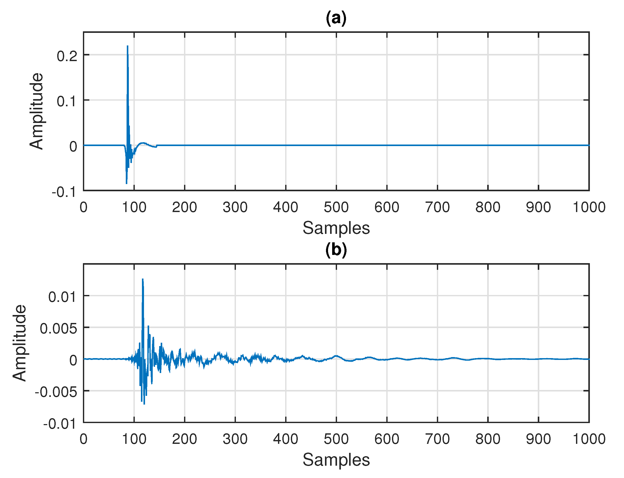
In the last set of experiments, two echo paths are considered in the context of an SISO system identification problem (i.e., echo cancellation scenario), following the discussion from Section 5. The length of both impulse responses is $\underline{L}=1000$. The first echo path (shown in Figure 2a) is a network impulse response from the ITU-T G168 Recommendation [40], i.e., the first cluster padded with zeros up to the length $\underline{L}$. The second echo path (depicted in Figure 2b) is a measured acoustic impulse response, which is available on-line at www.comm.pub.ro/plant (accessed on 5 March 2021).

In most of the experimental scenarios (i.e., MISO system identification), the proposed tensor-based algorithms, namely, LMS-T, NLMS-T, and RLS-T, are mainly compared to their conventional counterparts, i.e., LMS, NLMS, and RLS, respectively. In addition, in some of the experiments, the tensor LMS algorithm [7] is included in comparisons. In the last set of experiments (i.e., SISO system identification), the RLS-NKP [31] is compared to the conventional RLS algorithm.

In most of the experiments (i.e., MISO scenario), the performance measure is the normalized misalignment (in dB) for the identification of the global impulse response, which is evaluated as $20{\log }_{10}\left[{∥\mathbf{g}-\widehat{\mathbf{g}}\left(n\right)∥}_2/{∥\mathbf{g}∥}_2\right]$. In the second to last sets of experiments, this performance measure is evaluated as $20{\log }_{10}\left[{∥\mathbf{h}-\widehat{\mathbf{g}}\left(n\right)∥}_2/{∥\mathbf{h}∥}_2\right]$. In order to test the tracking capabilities of the algorithms, we also introduce an abrupt change of the system (in the middle of each simulation), by changing the sign of the coefficients of ${\mathbf{h}}_1$. Finally, in the last set of experiments (i.e., SISO scenario), the normalized misalignment is evaluated as $20{\log }_{10}\left[{∥\underline{\mathbf{h}}-\underline{\widehat{\mathbf{h}}}\left(n\right)∥}_2/{∥\underline{\mathbf{h}}∥}_2\right]$, according to the notation from Section 5. Here, we also introduce an abrupt change of the impulse response in the middle of each simulation, by changing the sign of the coefficients of $\underline{\mathbf{h}}$.

In the first set of experiments, we evaluate the performance of the LMS-T and LMS algorithms. The main challenge related to these algorithms is the selection of their step-size parameters. For example, in the case of the conventional LMS algorithm, the theoretical upper bound for its step-size is given by $2/\left(L{\sigma }_x^2\right)$, where ${\sigma }_x^2$ is the variance of the input signal [5]. However, for stability reasons, this value should be lower in practice. In our experiments, we set the step-sizes of the LMS-T and LMS algorithms in order to reach similar misalignment levels, so that we can fairly compare their performance in terms of the convergence rate and tracking. Furthermore, the largest step-size of the conventional LMS algorithm is set close to its stability limit, in order to provide the fastest convergence mode of the algorithm. Clearly, since the LMS-T algorithm combines the solutions of much shorter filters (of lengths $L_i,i=1,2,\dots ,N$), the corresponding values of its step-sizes are larger as compared to the step-size of the conventional LMS counterpart (with the length $L={\prod }_{i=1}^N{L}_i$).

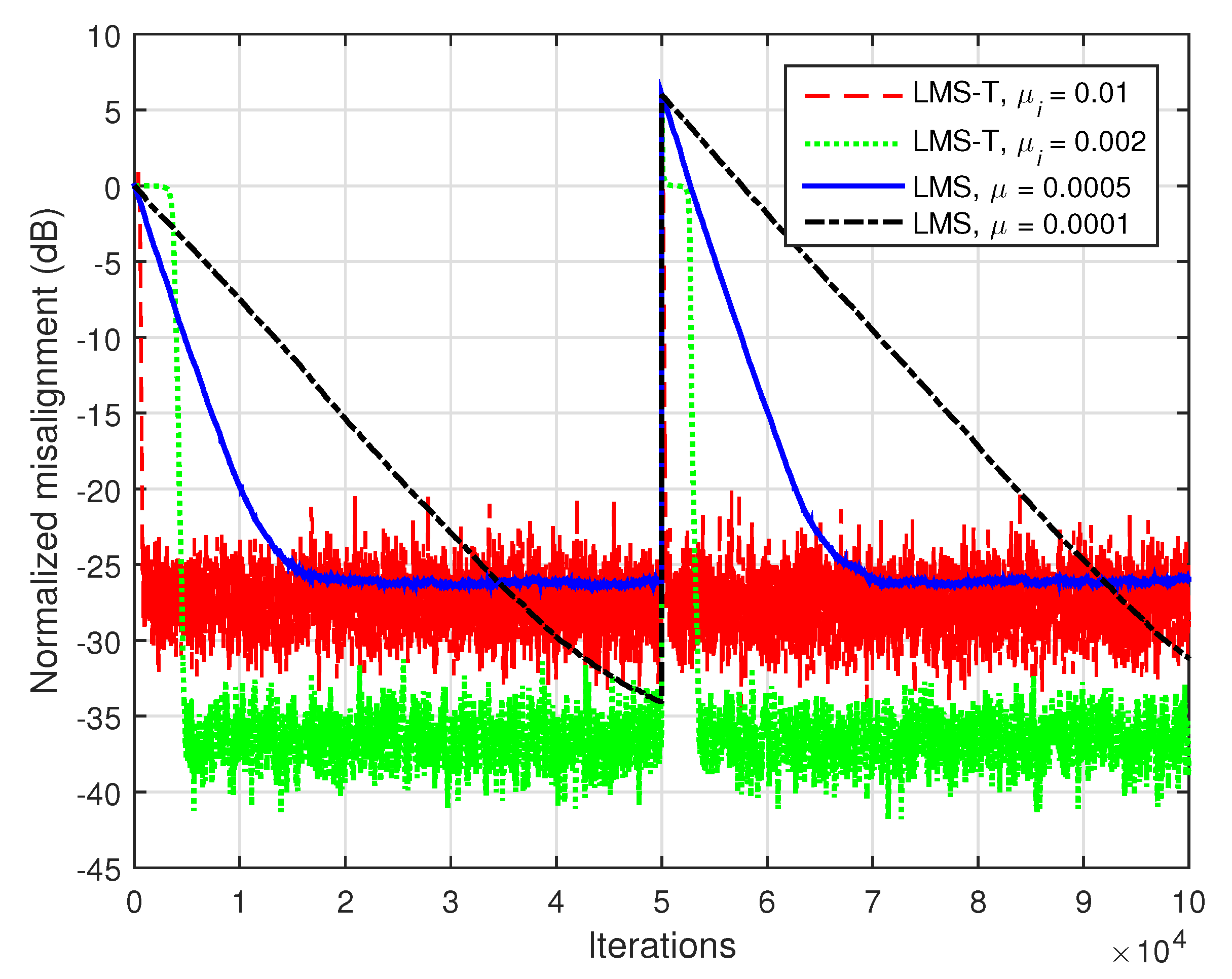
In Figure 3, we consider $N=4$ and we use white Gaussian noises as input signals. In this case, the length of the global impulse response is $L=2048$. As expected, a lower value of the step-size improves the misalignment but pays with a slower convergence rate and tracking. This is valid for both LMS-T and LMS algorithms. However, the LMS-T algorithm converges and tracks significantly faster than its conventional counterpart.

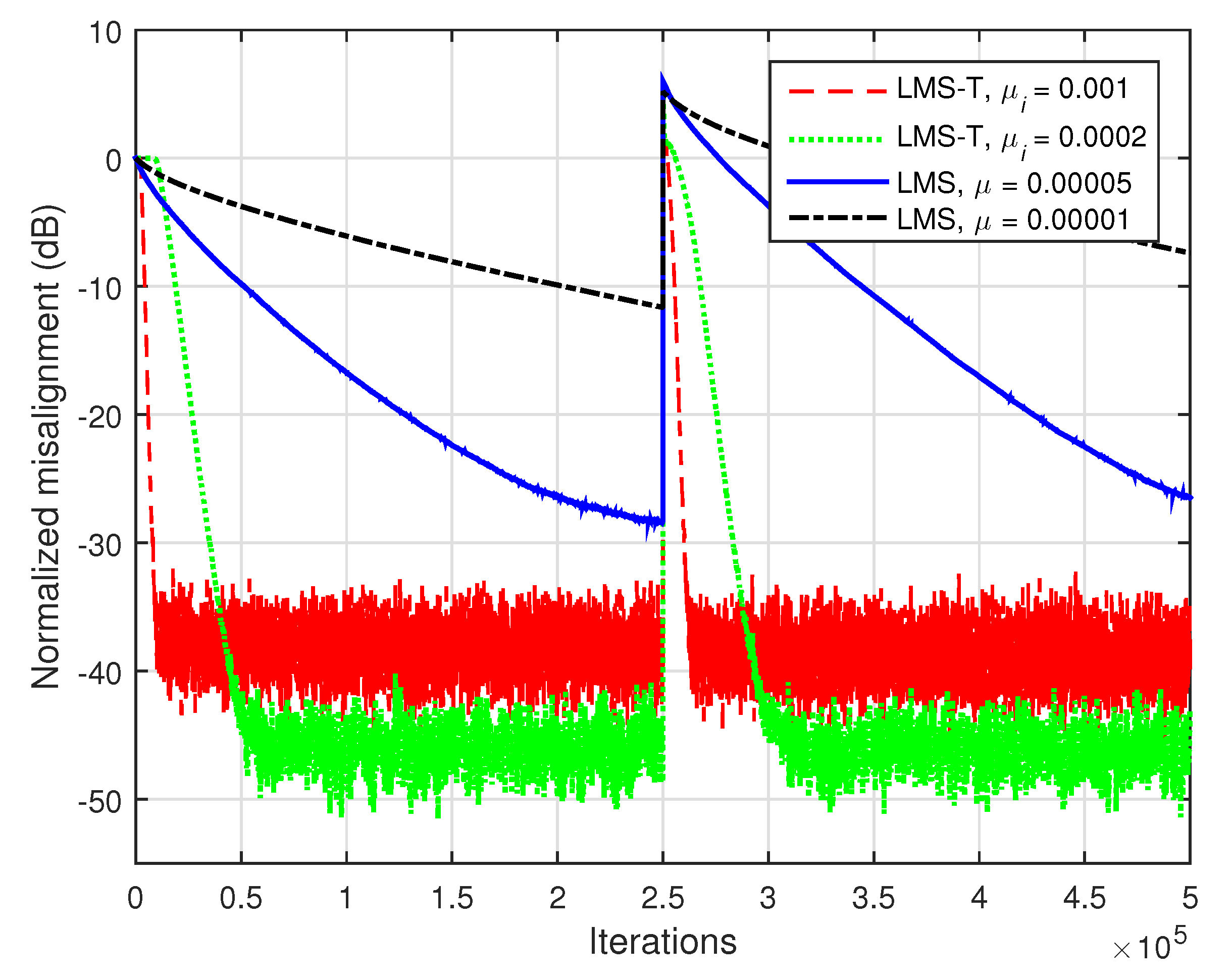
The gain is much more apparent in case of highly-correlated inputs. Such a scenario is considered in Figure 4, where $N=4$ and the input signals are AR(1) processes. As we can notice, the proposed LMS-T outperforms the conventional LMS algorithm in terms of both convergence rate/tracking and misalignment.

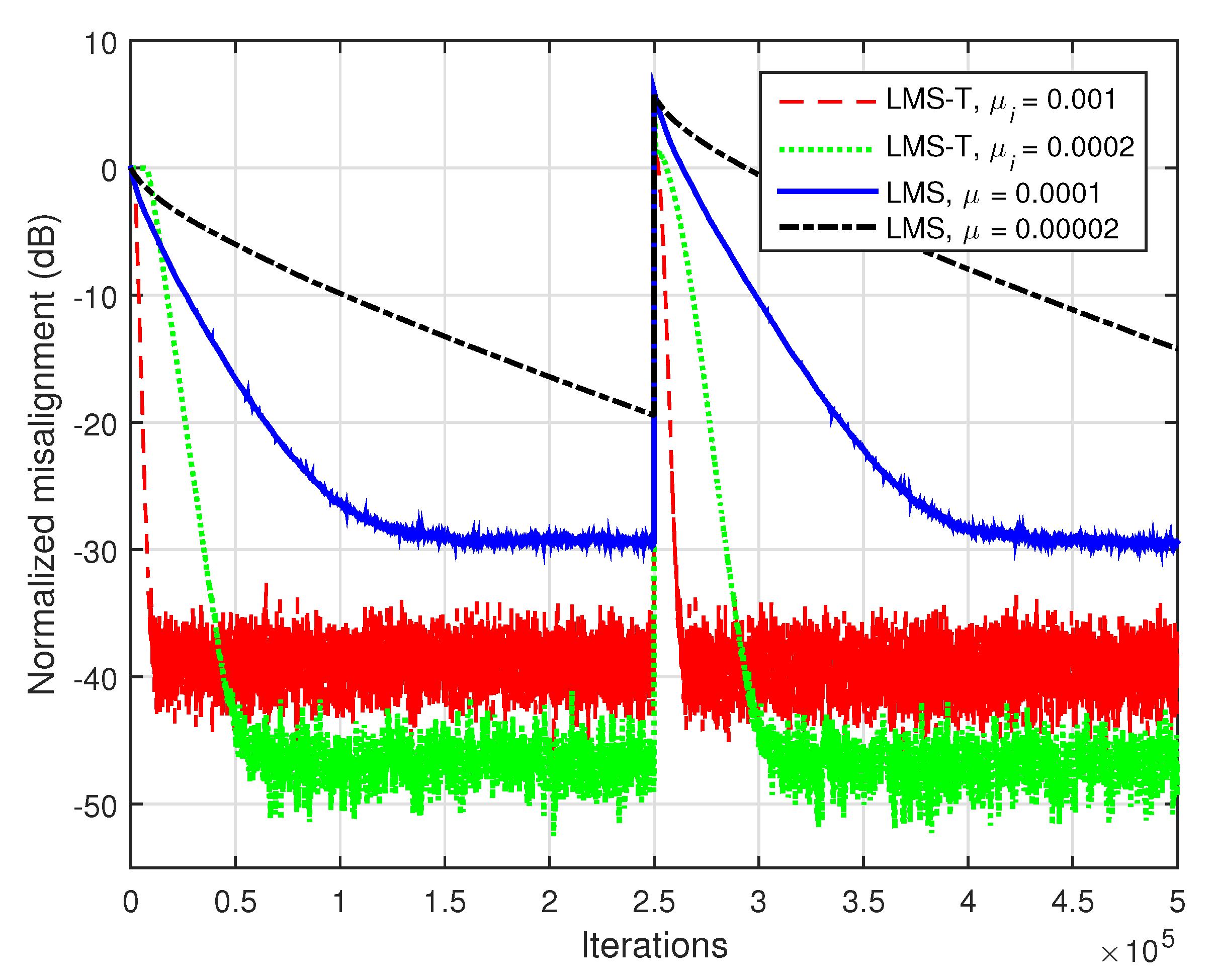
The performance gain of the LMS-T algorithm increases for higher orders, in comparison with the conventional LMS algorithm. This is supported in Figure 5, where the input signals are AR(1) processes and $N=5$, so that the length of the global impulse response is $L=4096$. The identification of such a long impulse response (especially using correlated inputs) is challenging for any conventional adaptive algorithm, highly influencing the convergence rate, tracking, and accuracy of the solution. It can be noticed that the LMS-T algorithm outperforms by far its conventional counterpart, in terms of all these performance criteria.

The second set of experiments is dedicated to the normalized versions, i.e., the NLMS-T and NLMS algorithms. The main advantage of these algorithms is related to the selection of the normalized step-sizes and, consequently, to their ability to operate in nonstationary conditions (related to the input and/or the environment). For example, the fastest convergence mode of the conventional NLMS algorithm is obtained when the normalized step-size is set to 1 [5]. Based on the theoretical findings related to the bilinear algorithms [22], setting the normalized step-sizes of the NLMS-T algorithm such that their sum is equal to 1 could lead to the same value of the misalignment as the conventional NLMS algorithm with the fastest convergence mode.

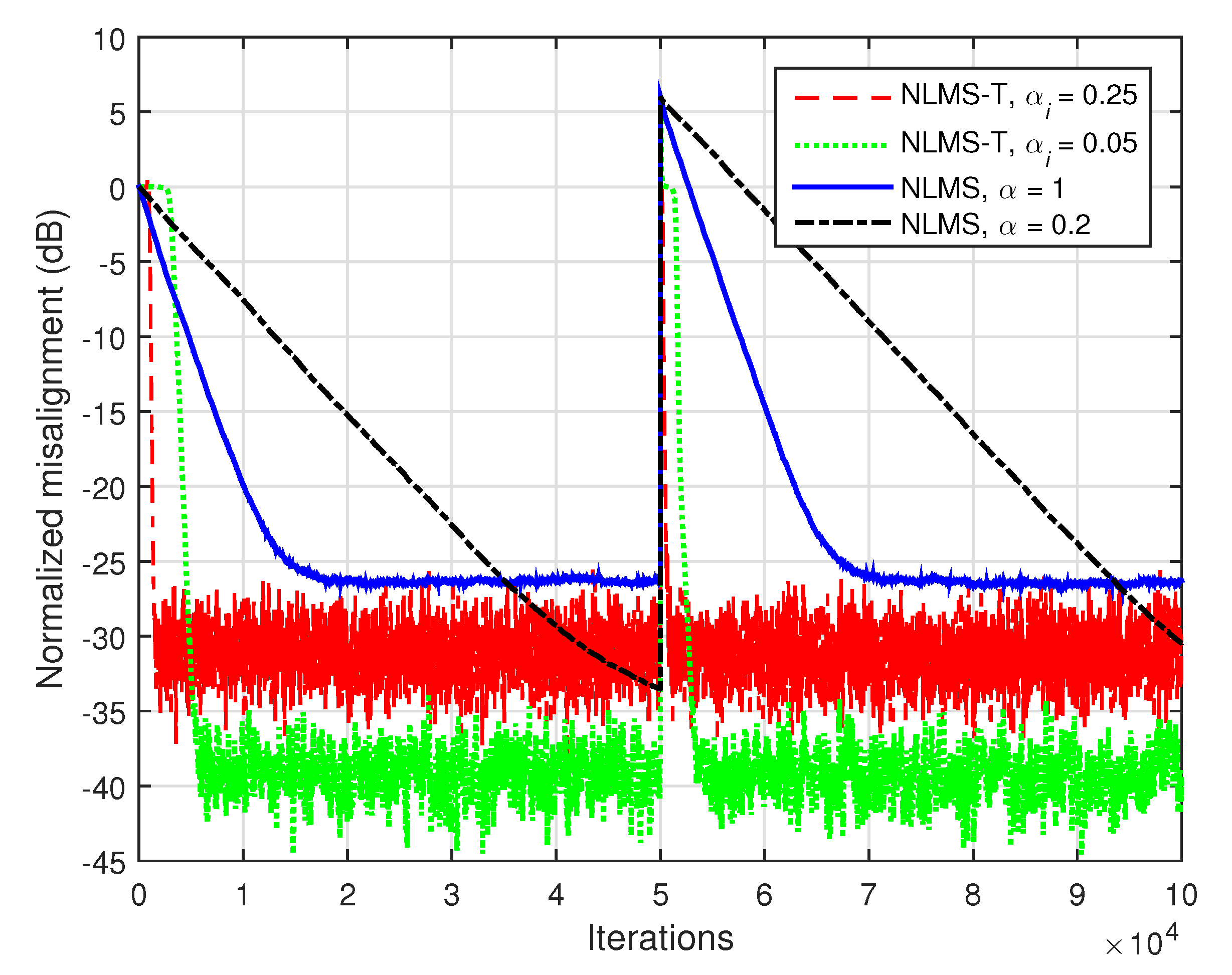
In Figure 6, the input signals are white Gaussian noises and $N=4$. Hence, the impulse responses are those indicated in Figure 1, with the global impulse response of length $L=2048$. The conclusions of this experiment are similar to those obtained in the case of the LMS algorithms (related to Figure 3). Most important, the NLMS-T algorithm significantly outperforms the conventional NLMS algorithm is terms of the convergence rate and tracking, especially for lower values of the normalized step-sizes.

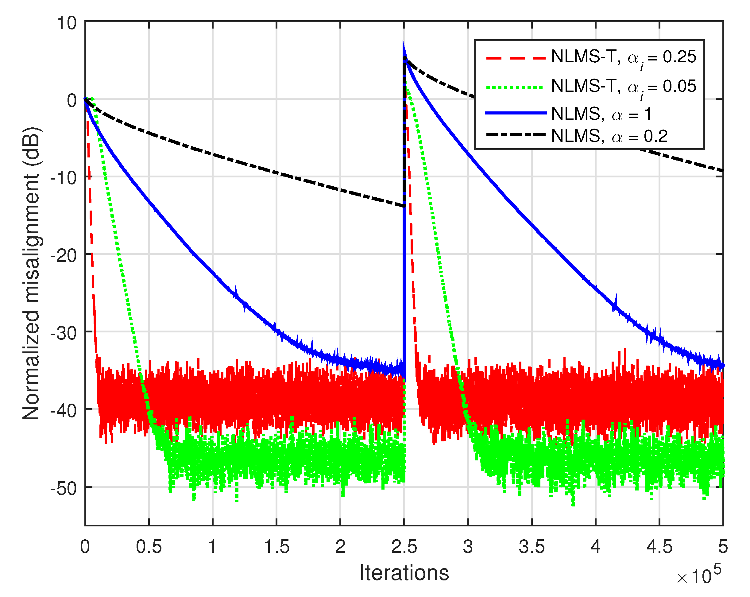
In addition, when the input signals are correlated, the gain of the proposed NLMS-T algorithm is even more apparent. This can be noticed in Figure 7, where the input signals are AR(1) processes. As we can see from this figure, the fastest convergence mode of the conventional NLMS algorithm is outperformed by far even by the NLMS-T algorithm using the lower normalized step-sizes.

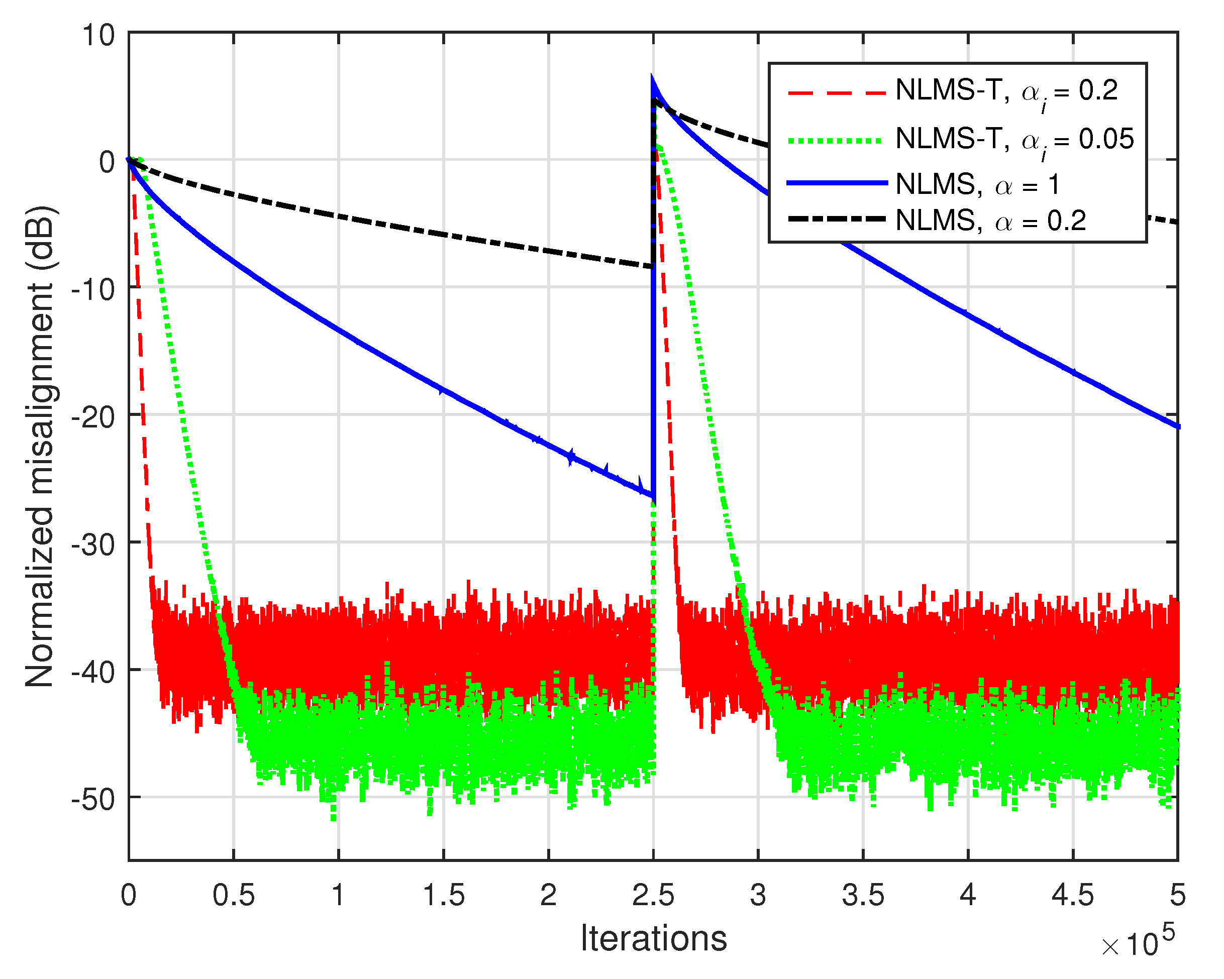
Increasing the system order also outlines the performance gain of the NLMS-T algorithm. This aspect is supported in Figure 8, where $N=5$ and the global impulse response has the length $L=4096$. As we can notice, the fastest convergence mode of the conventional NLMS algorithm does not reach the steady-state before the system changes, while the NLMS-T algorithm converges (and tracks) much faster, despite the values of its normalized step-sizes.

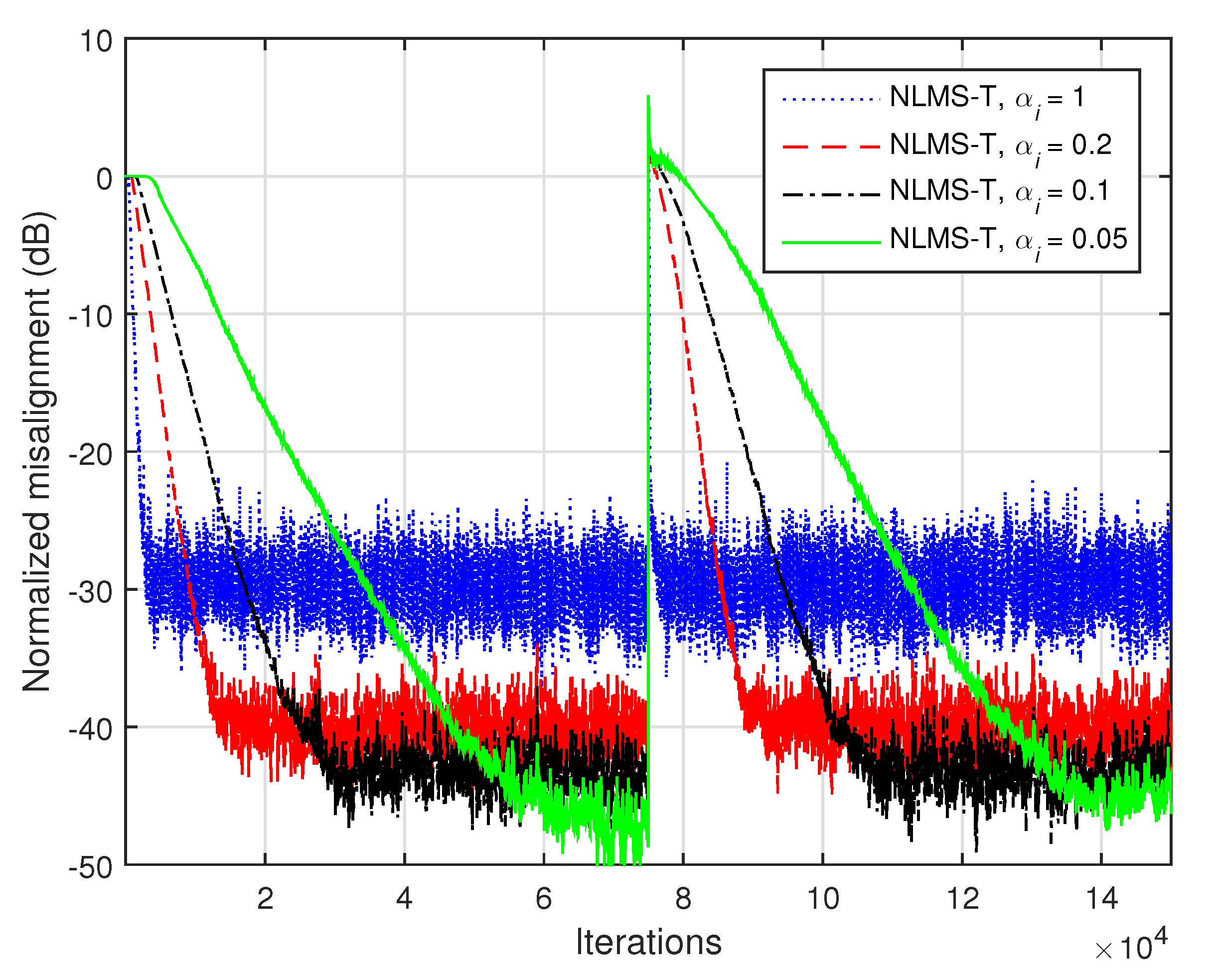
The influence of the normalized step-sizes on the performance of the NLMS-T algorithm is analyzed in Figure 9, where the input signals are AR(1) processes and $N=4$. As expected, higher values of the normalized step-sizes improve the convergence rate and tracking but increase the misalignment.

In the previous experiment, we used equal values of ${\alpha }_i$ ($i=1,2,\dots ,N$) for the individual filters. However, since these filters have different lengths, an alternative strategy would be to set different values of the normalized step-sizes for each individual filter. Such a scenario is considered in Figure 10, where we set ${\alpha }_1=0.25$ for the first filter (of length $L_1$), while varying the other normalized step-sizes ${\alpha }_j,j=2,3,4$. The other conditions are the same as in the previous experiment, i.e., $N=4$ and AR(1) inputs. We can notice the same compromise in terms of the main performance criteria (convergence rate/tracking versus misalignment). Consequently, several strategies to set these parameters can be adopted in different contexts, taking into account that the convergence features are mainly influenced by the longest individual filter [22].

The third set of experiments is dedicated to the RLS-based algorithms. The performance of these algorithms is mainly influenced by the forgetting factors [41]. In the case of the conventional RLS algorithm [5], the value of this parameter is usually set as $\lambda =1-1/\left(KL\right)$, where $K\ge 1$. A higher value of the forgetting factor (i.e., closer to 1) improves the misalignment, but significantly slows down the tracking reaction. A natural choice is to set the forgetting factors of the RLS-T algorithm using a similar strategy, such that ${\lambda }_i=1-1/\left(K{L}_i\right),i=1,2,\dots ,N$. Nevertheless, depending on the character and requirements of a particular application, different other strategies can be considered. For example, one can set all the forgetting factors equal to that associated to the longest filter. However, analyzing the impact of different strategies for the selection of the forgetting factors is beyond the scope of this paper.

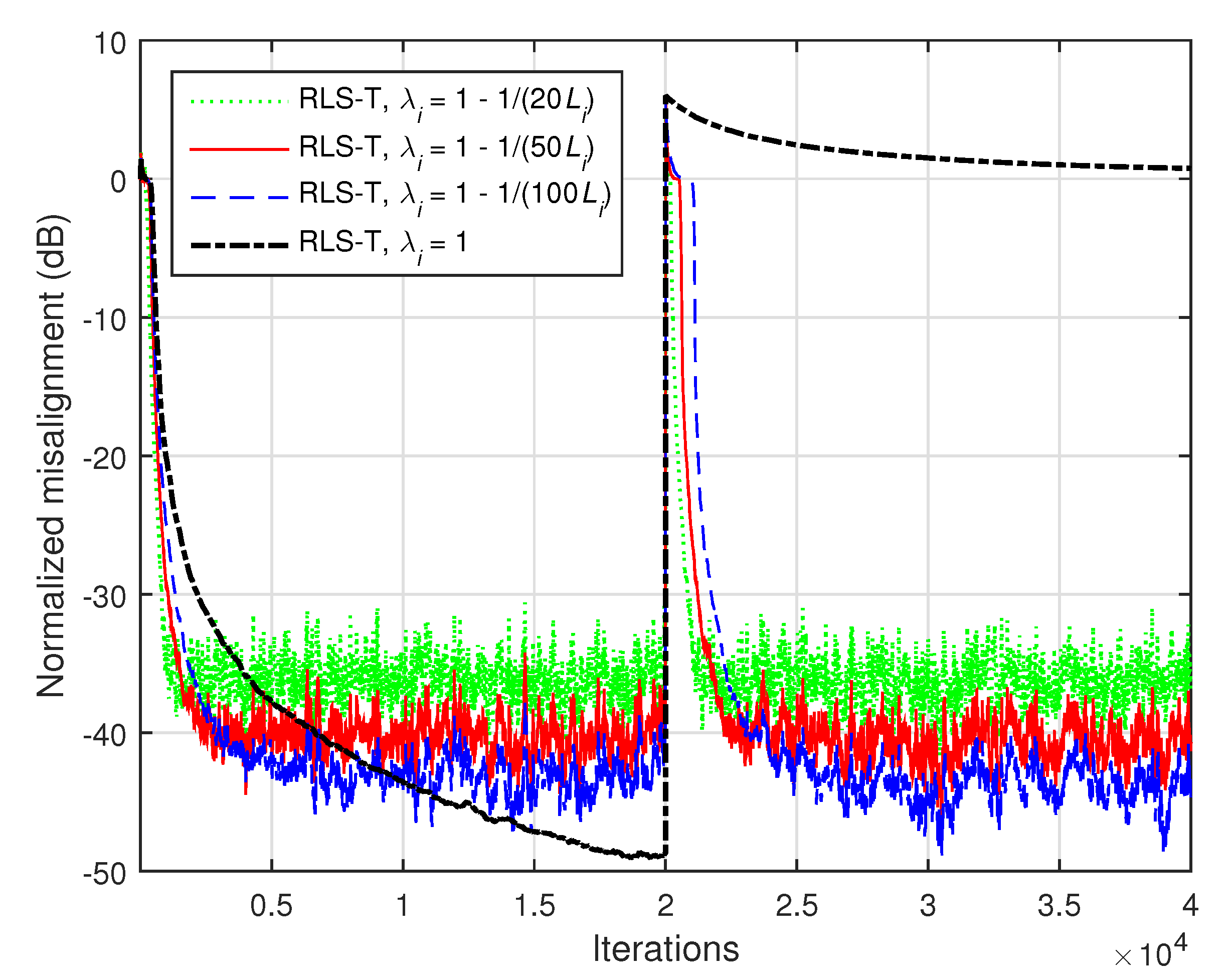
The influence of the forgetting factors on the performance of the proposed RLS-T algorithm is investigated in Figure 11. In this simulation, the input signals are white Gaussian noises and the system order is $N=4$ (i.e., the impulse responses from Figure 1). The forgetting factors are set based on the previous rule, i.e., ${\lambda }_i=1-1/\left(K{L}_i\right),i=1,2,\dots ,N$, using different values of K. As expected, increasing the values of the forgetting factors reduces the tracking capability of the algorithm but improves its accuracy by achieving a lower steady-state misalignment. Clearly, the lowest misalignment is obtained for ${\lambda }_i=1,i=1,2,\dots ,N$ (i.e., $K\to \infty$), while this produces the slowest tracking reaction.

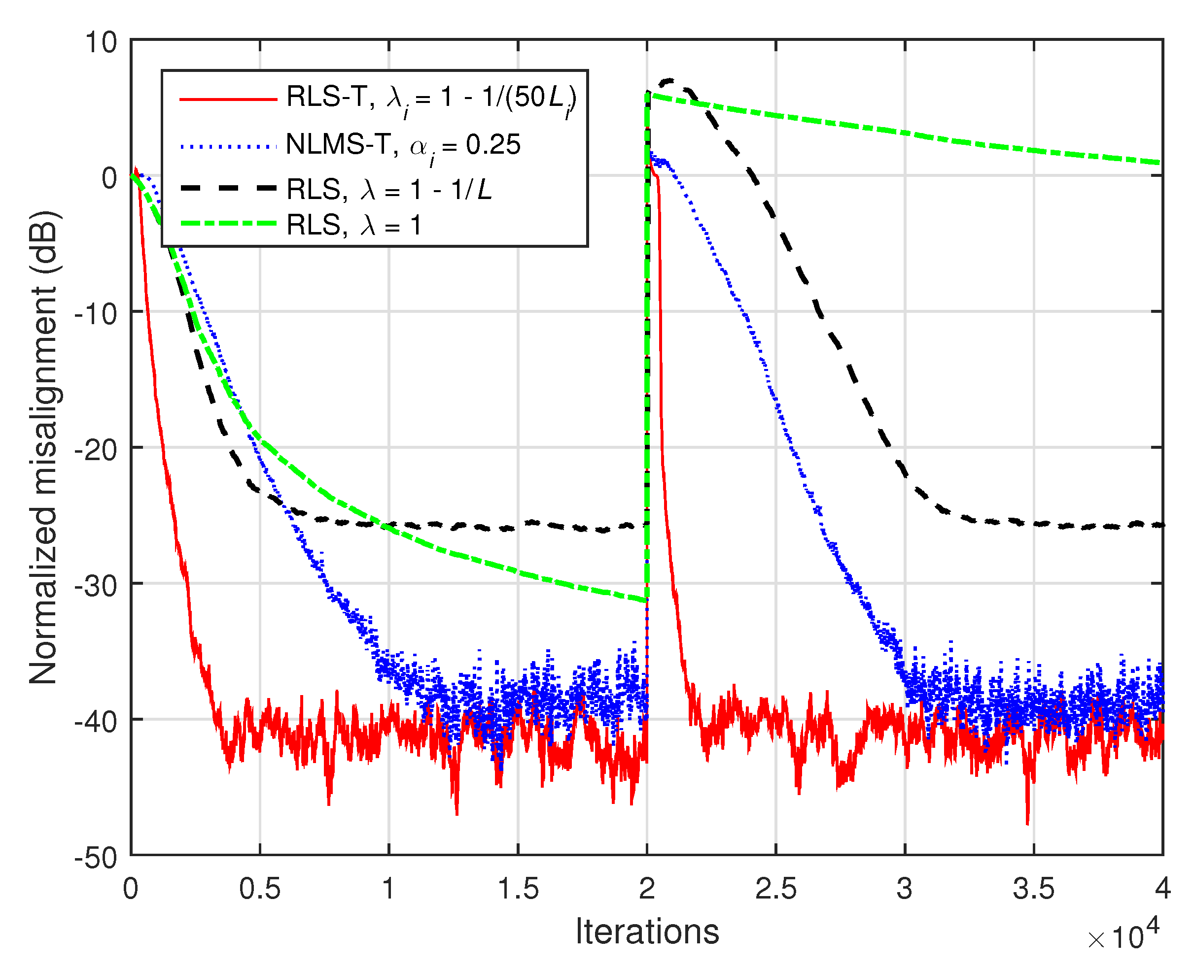
The computational complexity of the conventional RLS algorithm (which is proportional to $L^2$) makes it prohibitive for the identification of long length impulse responses, especially in real-time applications and taking into account the implementation costs. On the other hand, due to the decomposition feature and the operation with shorter impulse responses, the proposed RLS-T algorithm could be more suitable in such scenarios. In addition, due to the fact that the filter’s length has an influence on the main performance criteria (e.g., convergence rate/tracking and accuracy), the RLS-T algorithm outperforms its conventional counterpart. This is supported in Figure 12, where the conventional RLS algorithm is used as benchmark. Furthermore, the NLMS-T algorithm is introduced in comparisons. In this simulation, the input signals are AR(1) processes and $N=4$, while the length of the global impulse response is $L=2048$. As we can notice, the initial convergence rate of the conventional RLS algorithm using a lower value of the forgetting factor ($\lambda =1-1/L$) is similar to that obtained by the NLMS-T algorithm. On the other hand, the tracking reaction of the RLS algorithm is slower as compared to the NLMS-T algorithm, while its steady-state misalignment is higher. A lower misalignment level could be achieved by the RLS algorithm with the maximum forgetting factor (i.e., $\lambda =1$), but paying with the slowest tracking capability. It can be noticed that the proposed RLS-T algorithm clearly outperforms all the other algorithms involved in comparisons.

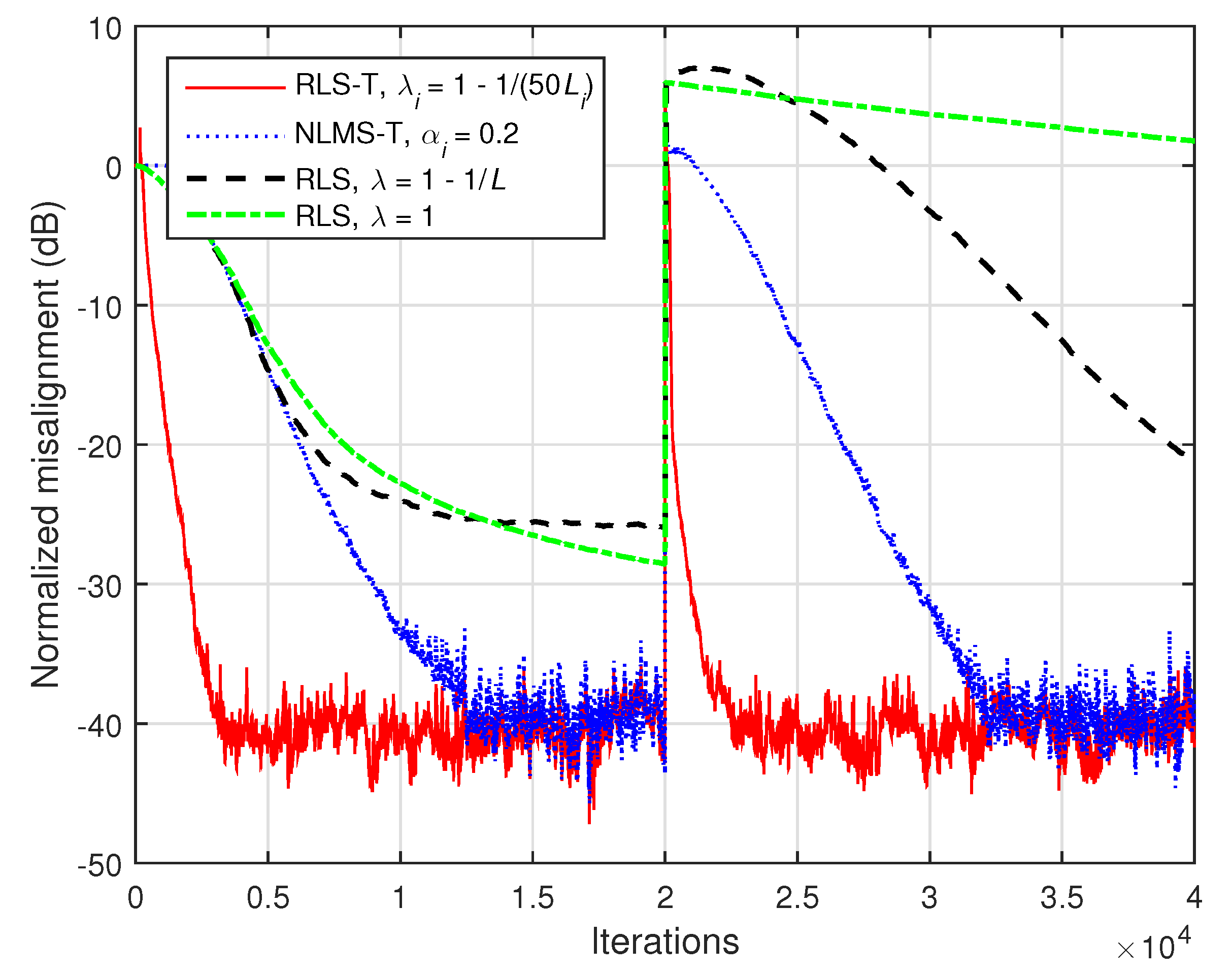
Next, the previous algorithms are compared in a more challenging scenario, using $N=5$ and $L=4096$, while the input signals are AR(1) processes. Such a filter length is excessively high for the conventional RLS algorithm. The results provided in Figure 13 show that the NLMS-T algorithm outperforms the conventional RLS algorithm in this scenario. As expected, the RLS-T algorithm achieves a faster convergence rate and tracking reaction as compared to the NLMS-T algorithm.

We should also outline that in the last two simulations (Figure 12 and Figure 13), the main parameters of the RLS-T and NLMS-T algorithms (i.e., ${\lambda }_i$ and ${\alpha }_i$, respectively) are set to achieve the same steady-state misalignment level. However, as previously shown in Figure 11, using higher values for the forgetting factors of the RLS-T algorithm would further improve the misalignment level, paying with a slightly reduced convergence rate and tracking.

In the next set of experiments, we consider a more general scenario where the impulse response of the system is not perfectly separable. Hence, it is generated as $\mathbf{h}=\mathbf{g}+\mathbf{f}$, where $\mathbf{g}$ is obtained as described in the beginning of this section (e.g., see Figure 1), while $\mathbf{f}$ is randomly generated (with Gaussian distribution) and its variance is set to $\zeta {∥\mathbf{g}∥}_2/L$, where $\zeta >0$. Clearly, a higher value of $\zeta$ makes the separation more challenging. In this set of experiments, we consider AR(1) processes as inputs. In addition, we include in comparisons a counterpart of the NLMS-T algorithm, i.e., the tensor LMS developed in [7]. The step-sizes of this algorithm are evaluated as ${\mu }_i\left(n\right)={\alpha }_i/\left[{\delta }_i+{\sum }_{i=1}^N{\mathbf{x}}_{{\widehat{\mathbf{h}}}_i}^T\left(n\right){\mathbf{x}}_{{\widehat{\mathbf{h}}}_i}\left(n\right)\right],i=1,2,\dots ,N$, while the NLMS-T algorithm is updated based on (30). In the following experiments, we used the same values of ${\alpha }_i$ and ${\delta }_i$ for both algorithms. As a benchmark, we also evaluate the performance of the conventional RLS algorithm using $\lambda =1-1/L$.

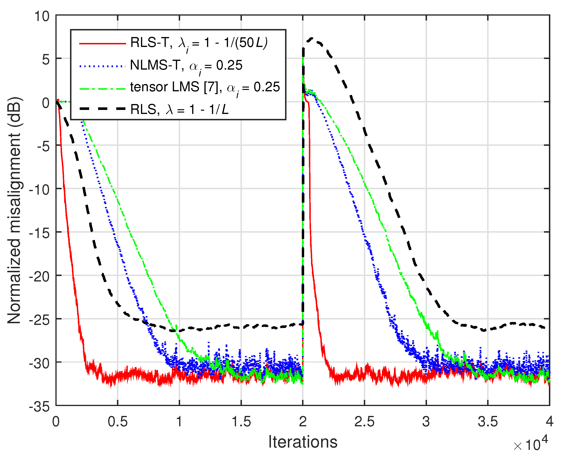
First, in Figure 14, we consider $N=4$ and $\zeta =0.001$. As we can notice, the misalignment of the tensor-based algorithms increases in this case (e.g., as compared to the results reported in Figure 12), since the nonseparable part of the system cannot be modeled. However, the RLS-T algorithm still achieves a faster convergence rate as compared to the conventional RLS algorithm. The convergence rate of the tensor LMS algorithm [7] is slightly slower as compared to the NLMS-T algorithm, while reaching a similar misalignment level. We can also notice that both algorithms outperform the conventional RLS algorithm in terms of tracking.

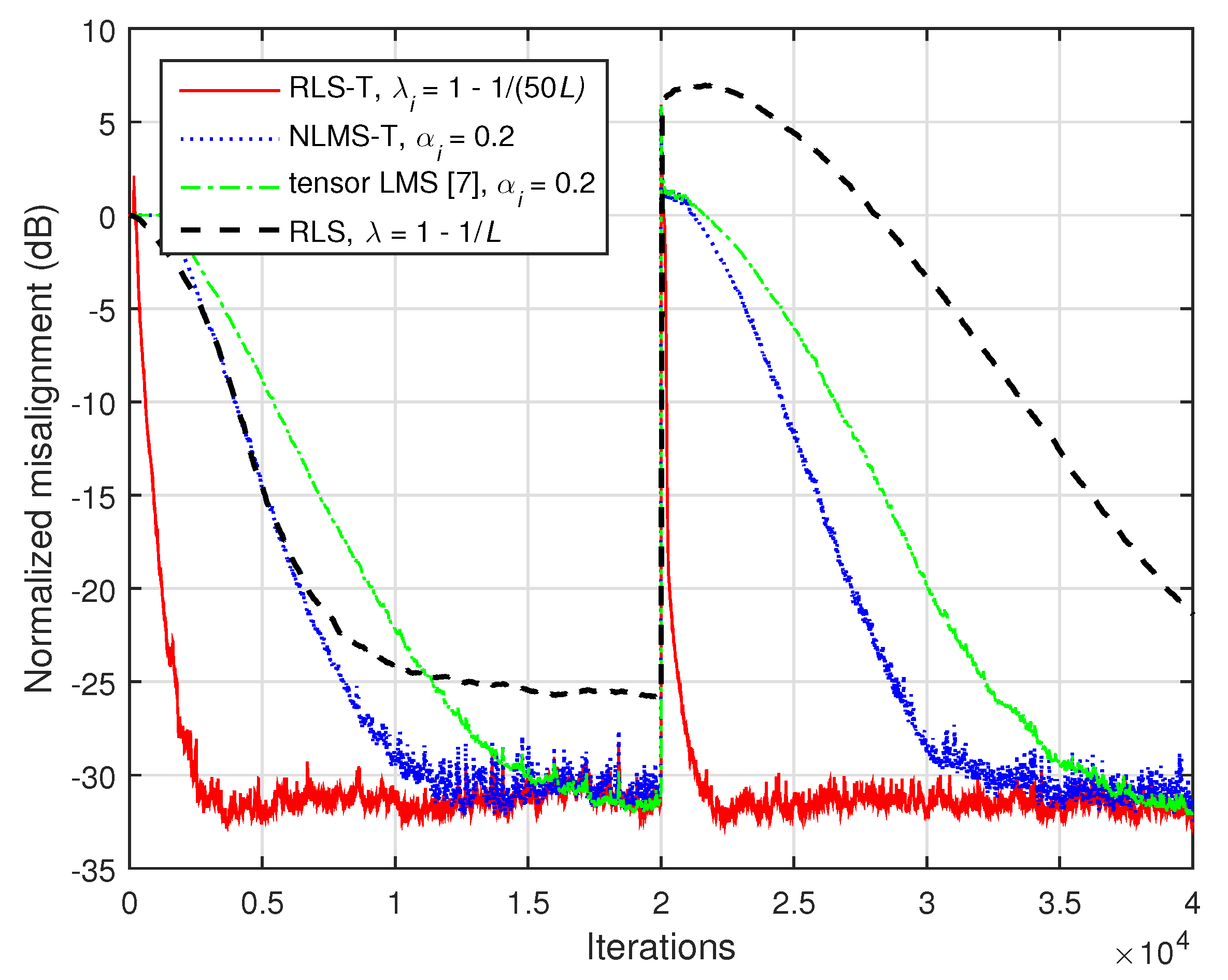
The gain is even more apparent for a higher order of the system, as supported in Figure 15, where $N=5$ and $\zeta =0.001$. Here, we can also notice that the performance of the NLMS-T algorithm is improved as compared to the tensor LMS algorithm [7], in terms of both convergence rate and tracking. As expected, the RLS-T algorithm outperforms by far all the other algorithms.

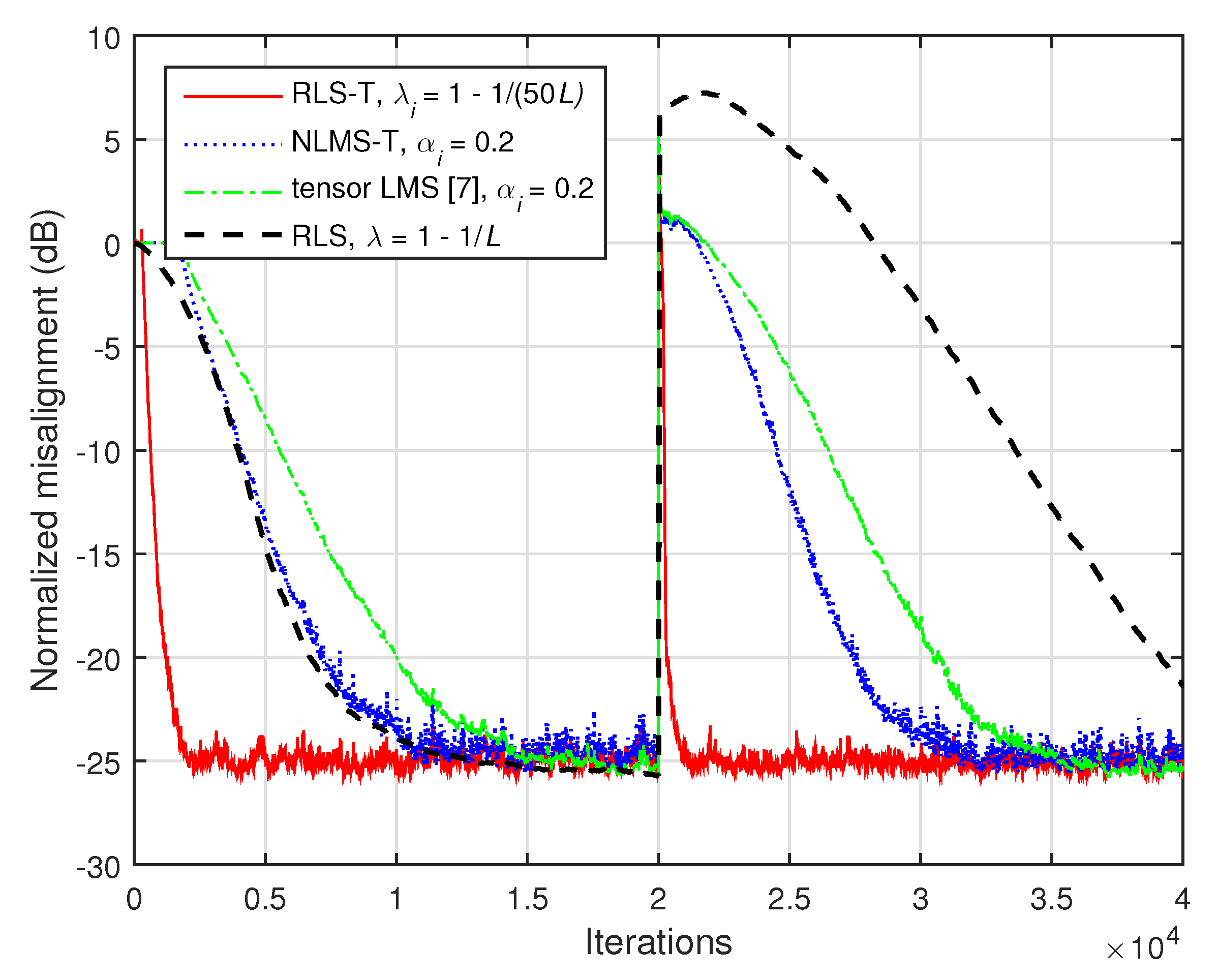
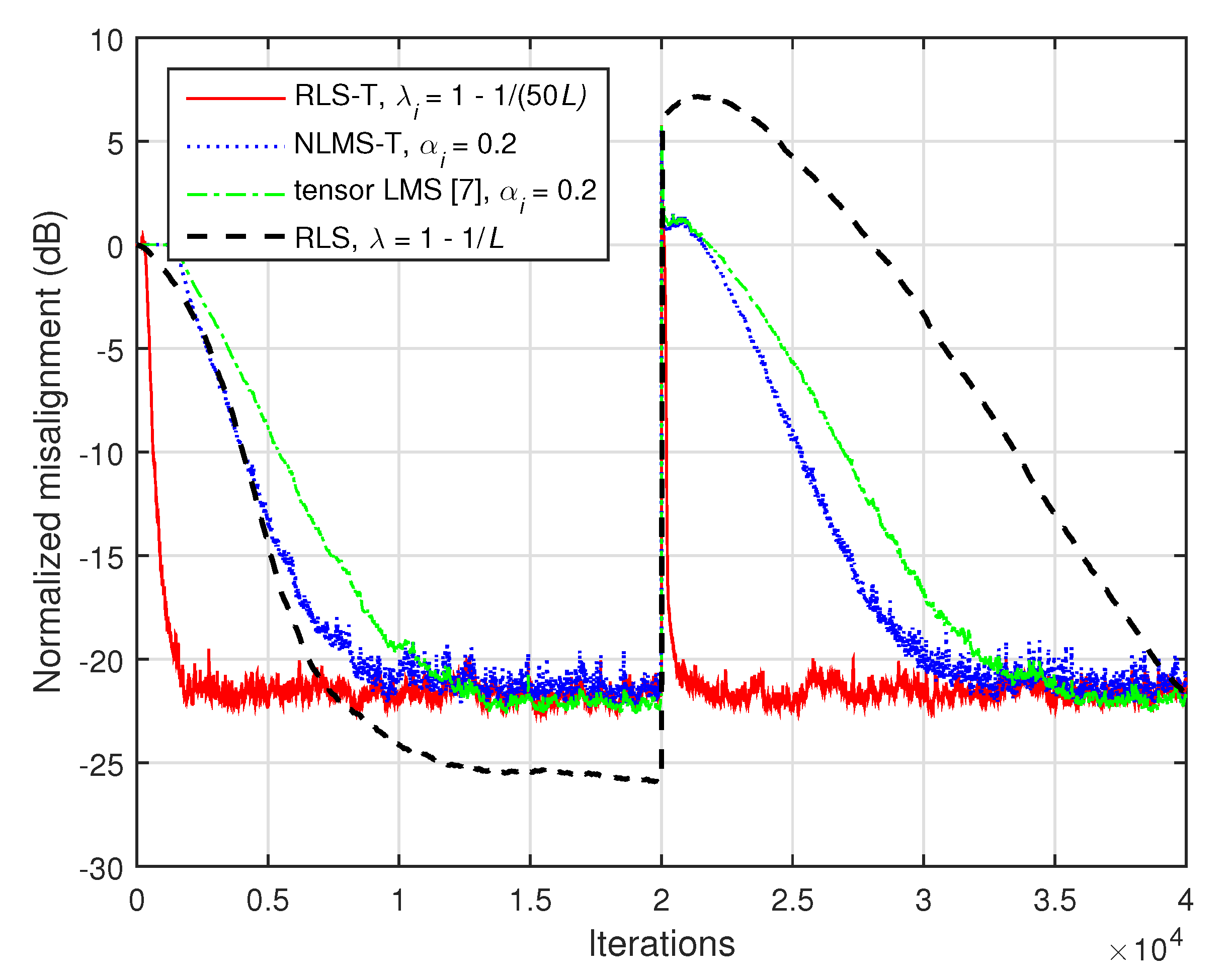
Further, in Figure 16 and Figure 17, the previous experiment is repeated, but using $\zeta =0.005$ and $\zeta =0.01$, respectively. Since the influence of the nonseparable part of the system is higher in these cases, the tensor-based algorithms reach a higher misalignment level. On the other hand, they still outperform the conventional RLS algorithm, especially in terms of the tracking capability.

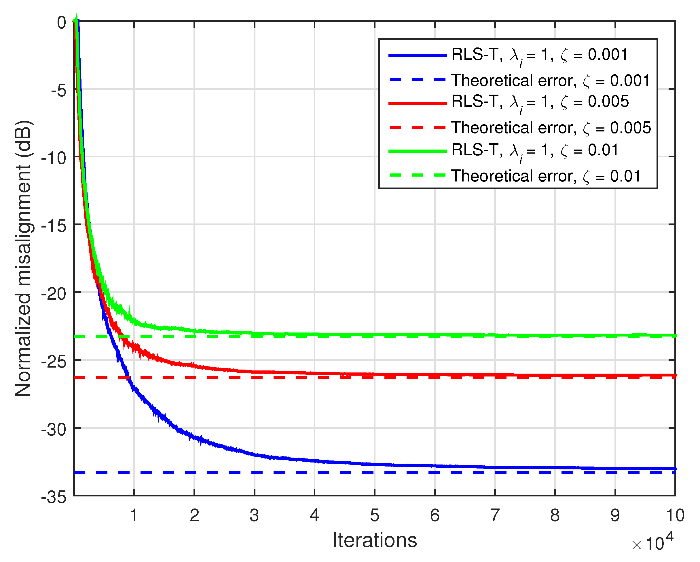
The nonseparable part of the system acts like an additional noise (which cannot be modeled based on the rank-1 decomposition), thus influencing the accuracy of the solution provided by the tensor-based algorithms. In this case, the theoretical error (in terms of the normalized misalignment) results in $20{\log }_{10}\left[{∥\mathbf{f}∥}_2/{∥\mathbf{h}∥}_2\right]$. In order to outline this behavior, we evaluate the performance of the RLS-T algorithm using ${\lambda }_i=1,i=1,2,\dots ,N$, for different values of $\zeta$. It is known that the RLS-based algorithms using the maximum value of the forgetting factor reach the lowest misalignment level, i.e., the highest accuracy of the solution [5,41]. In Figure 18, the input signals are AR(1) processes, $N=5$, and $L=4096$, while the theoretical errors are marked with dashed lines and appropriate colors. As expected, the error increases with the value of $\zeta$, while the misalignment of the RLS-T algorithm matches very well the theoretical threshold in each case. The overall behavior is similar to the under-modeling scenario [42], where the length of the adaptive filter is shorter as compared to the length of the unknown impulse response. Therefore, the “tail” of the impulse response that cannot be modeled acts like an additional noise, also increasing the misalignment level.

The last set of experiments is dedicated to the SISO system identification problem described in Section 5, which aims to go beyond the rank-1 decomposition approach. This represents the main motivation for future developments of the tensor-based adaptive filtering algorithms. In this framework, the RLS-NKP [31] is basically an extension of the RLS-T algorithm for $N=2$, which is suitable for the identification of more general forms of impulse responses. In these experiments, we consider an echo cancellation scenario, using the echo paths from Figure 2 (of length $\underline{L}={\underline{L}}_1{\underline{L}}_2=1000$). The RLS-NKP algorithm uses ${\underline{L}}_1=40$ and ${\underline{L}}_2=25$, while its forgetting factors are set to ${\underline{\lambda }}_1=1-1/\left(10P{\underline{L}}_1\right)$ and ${\underline{\lambda }}_2=1-1/\left(10P{\underline{L}}_2\right)$, with $P<{\underline{L}}_2$. Similarly, for a fair comparison, the forgetting factor of the conventional RLS algorithm is set to $\lambda =1-1/\left(10\underline{L}\right)$. Nevertheless, the computational complexity of the conventional benchmark is proportional to $\mathcal{O}\left({\underline{L}}^2\right)=\mathcal{O}\left({\underline{L}}_1^2{\underline{L}}_2^2\right)$, while the RLS-NKP algorithm requires a computational amount of $\mathcal{O}[{\left(P{\underline{L}}_1\right)}^2+{\left(P{\underline{L}}_2\right)}^2]$, which is much more advantageous for $P\ll {\underline{L}}_2$.

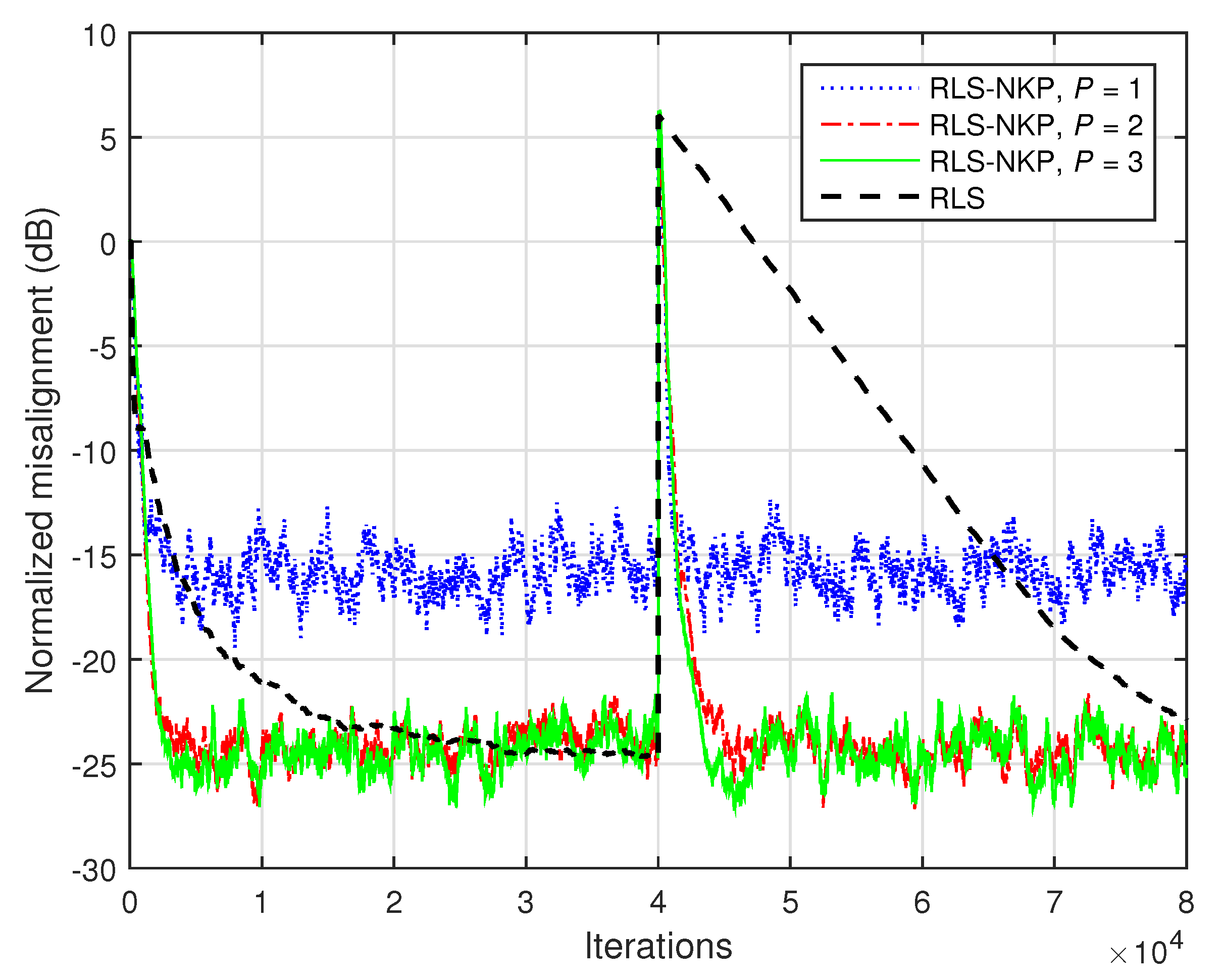
In Figure 19, the identification of the network impulse response from Figure 2a is evaluated. The input signal is a highly correlated AR(1) process and $\mathrm{ENR}=20$ dB. The RLS-NKP algorithm uses different values of $P\ll {\underline{L}}_2$. As shown in Section 5, this algorithm combines the estimates of two shorter filters of length $P{\underline{L}}_1$ and $P{\underline{L}}_2$, while the conventional RLS algorithm involves a single (long) adaptive filter of length $\underline{L}={\underline{L}}_1{\underline{L}}_2$. Consequently, the tracking reaction of the RLS algorithm is much slower as compared to the RLS-NKP, as we can notice in Figure 19. Furthermore, it should be noticed that a very small value of P (e.g., $P=2$) leads to an accuracy of the solution (i.e., misalignment level) similar to the conventional RLS algorithm. On the other hand, the computational complexity of the RLS-NKP algorithm is much lower in this case.

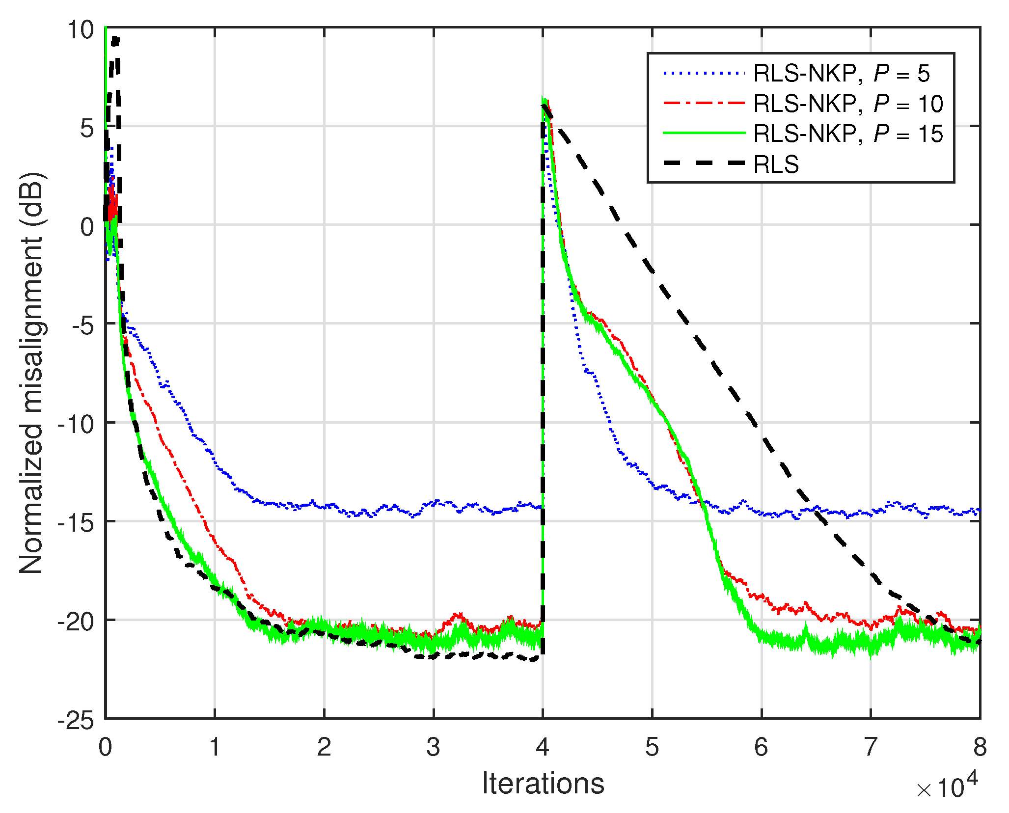
The previous experiment is repeated in Figure 20 but uses the acoustic impulse response from Figure 2b. As expected, the low-rank approximation is more challenging in this case, since the matrix $\underline{\mathbf{H}}$ is closer to full-rank. Consequently, the value of P should be increased. However, a moderate value of P (as compared to ${\underline{L}}_2$) is sufficient for the RLS-NKP algorithm, in order to reach a misalignment level close to the conventional RLS algorithm, while outperforming its counterpart in terms of the tracking capabilities.

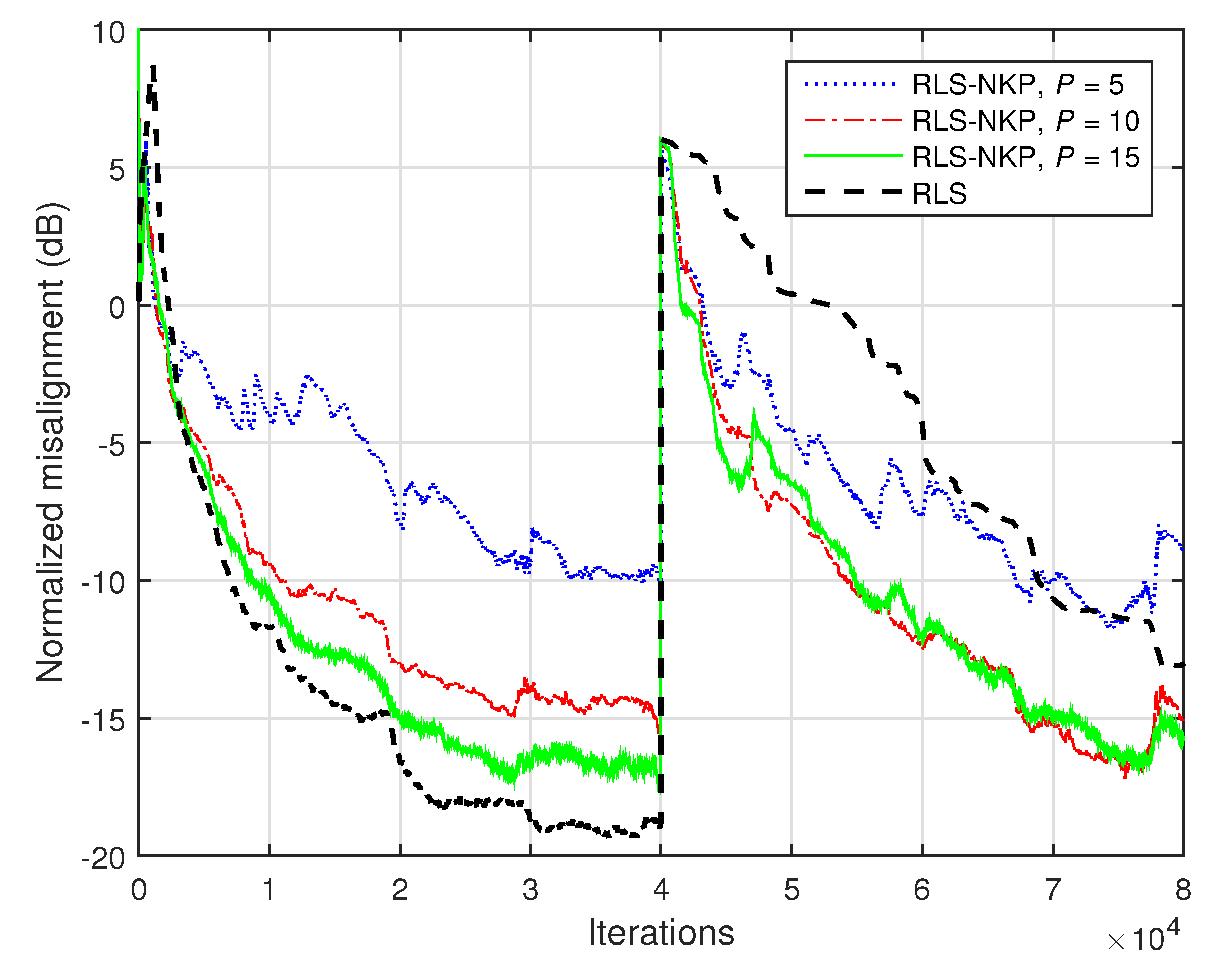
Finally, in Figure 21, the identification of the acoustic impulse response from Figure 2b is evaluated when using a speech signal as input. The nonstationary character of the speech signal represents a challenge for any adaptive algorithm. Nevertheless, the tracking capability of the RLS-NKP is still better as compared to the conventional RLS algorithm.

As explained in Section 5, the RLS-NKP exploits a low-rank approximation approach and represents an extension of the RLS-T algorithm for $N=2$. Thus, it is efficient for the identification of more general forms of impulse responses, in the context of SISO scenarios. On the other hand, the RLS-T algorithm is developed based on the decomposition of rank-1 tensors, in the framework of a MISO system identification problem. Therefore, it is suitable when dealing with linearly separable systems, e.g., [8,10,14], even affected by a nonseparable part. Concluding, an extension of the RLS-T algorithm for higher-rank ($R\ge 3$) and higher-order tensors ($N\ge 3$) could inherit the advantages of the decomposition-based approach and the applicability features of the low-rank approximation method.

7. Conclusions and Future Works

In this paper, we have presented a family of tensor-based adaptive filtering algorithms, targeting an efficient way to solve high-dimension MISO system identification problems. The main feature of this solution is the decomposition-based approach, which allows us to deal with the individual components of a high-order tensor, instead of following the conventional approach that only focuses on the identification of the system global impulse response. In other words, the tensor-based algorithms combine the solutions of N shorter filters (where N is the tensor order) in order to estimate the global impulse response. Consequently, since the filter length influences the performance of any adaptive algorithm, the proposed solutions outperform the conventional methods in terms of the main performance criteria, thus providing faster convergence rate/tracking and lower misadjustment.

The resulting tensor-based algorithms, namely, LMS/NLMS-T and RLS-T, have been built on the two main categories of adaptive filters, which are based on the minimization of the mean-squared error and least-squares criteria, respectively. Among them, the RLS-T algorithm outperforms its LMS-based counterparts, especially in terms of convergence rate and tracking. In perspective, the RLS-T algorithm could be combined with line searching techniques (e.g., the dichotomous coordinate descent iterations), in order to further improve its computational efficiency. Furthermore, it would be interesting to explore a solution based on different combinations of adaptive filters, thus using different types of algorithms to model the individual components that form the global estimate. In this way, we could further exploit the particularities and advantages of each category of adaptive algorithms, in order to improve the overall performance. Furthermore, extending the approach in case of higher rank tensors could lead to improved identification methods, which could be efficiently applied when dealing with more general forms of impulse responses, especially of long length.