Integration of Dirac’s Efforts to Construct a Quantum Mechanics Which is Lorentz-Covariant


1
Center for Fundamental Physics, University of Maryland, College Park, MD 20742, USA
2
Department of Radiology, New York University, New York, NY 10016, USA
*
Author to whom correspondence should be addressed.
†
Both authors contributed equally to this work.
Symmetry 2020, 12(8), 1270; https://doi.org/10.3390/sym12081270
Submission received: 24 June 2020
/
Revised: 16 July 2020
/
Accepted: 29 July 2020
/
Published: 1 August 2020
(This article belongs to the Section Physics)
Abstract
:The lifelong efforts of Paul A. M. Dirac were to construct localized quantum systems in the Lorentz covariant world. In 1927, he noted that the time-energy uncertainty should be included in the Lorentz-covariant picture. In 1945, he attempted to construct a representation of the Lorentz group using a normalizable Gaussian function localized both in the space and time variables. In 1949, he introduced his instant form to exclude time-like oscillations. He also introduced the light-cone coordinate system for Lorentz boosts. Also in 1949, he stated the Lie algebra of the inhomogeneous Lorentz group can serve as the uncertainty relations in the Lorentz-covariant world. It is possible to integrate these three papers to produce the harmonic oscillator wave function which can be Lorentz-transformed. In addition, Dirac, in 1963, considered two coupled oscillators to derive the Lie algebra for the generators of the de Sitter group, which has ten generators. It is proven possible to contract this group to the inhomogeneous Lorentz group with ten generators, which constitute the fundamental symmetry of quantum mechanics in Einstein’s Lorentz-covariant world.
Keywords:
Dirac’s relativistic quantum mechanics; Lorentz-covariant harmonic oscillators; special relativity from the Heisenberg bracketsPACS:
03.65.Fd; 03.67.-a; 05.30.-d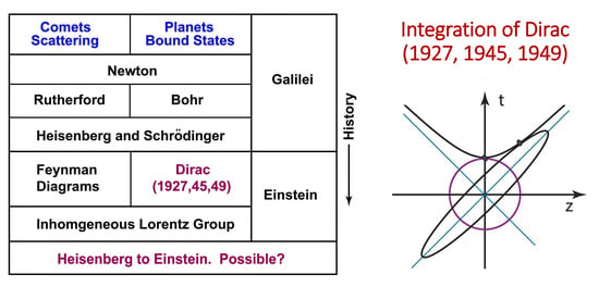
1. Introduction
Since 1973 [1], the present authors have been publishing papers on the harmonic oscillator wave functions which can be Lorentz-boosted, leading to a number of books [2,3,4,5]. We noticed that the Gaussian form of the wave function undergoes an elliptic space-time deformation when Lorentz-boosted, leading to the correct proton form factor behavior for large momentum transfers.
It was then noted that the harmonic oscillator functions exhibit the contraction and orthogonality properties quite consistent with known rules of special relativity and quantum mechanics [6,7].
In 1977, using the Lorentz-covariant wave functions, the present authors showed that Gell-Mann’s quark model [8] for the hadron at rest and Feynman’s parton model for fast-moving hadrons [9] are two different manifestations of one Lorentz-covariant entity [10,11].
In 1979 [12], it was shown that the oscillator system we constructed can be used for a representation of the Lorentz group, particularly Wigner’s -like little group for massive particles [13]. More recently, it was shown that these oscillator wave functions can serve as squeezed states of light and Gaussian entanglement [14,15,16].
In 1983, it became known that, if the speed of a spin-1 particle reaches that of light, the component of spin in the direction of its momentum remains invariant as its helicity, but the spin components perpendicular to the momentum become one gauge degree of freedom [17,18]. Indeed, this result allows us to include our oscillator-based quark-parton picture as further content of Einstein’s [11], as shown in Table 1.
The purpose of the present paper is to show that the harmonic oscillator wave functions we have studied since 1973 can serve another purpose. It is possible to obtain this covariant form of relativistic extended particles by integrating the three papers Dirac wrote, as indicated in Table 1.
- In 1927, Dirac pointed out that the time-energy uncertainty should be considered if the system is to be Lorentz-covariant [19].
- In 1945, Dirac said the Gaussian form could serve as a representation of the Lorentz group [20].
- In 1949, when Dirac introduced both his instant form of quantum mechanics and his light-cone coordinate system [21], he clearly stated that finding a representation of the inhomogeneous Lorentz group was the task of Lorentz-covariant quantum mechanics.
- In 1963, Dirac used the symmetry of two coupled oscillators to construct the group [22].
In the fourth paper published in 1963, Dirac considered two coupled oscillators using step-up and step-down operators. He then constructed the Lie algebra (closed set of commutation relations for the generators) of the de Sitter group, also known as , using ten quadratic forms of those step-up and step-down operators. The harmonic oscillator is a language of quantum mechanics while the de Sitter group is a language of the Lorentz group or Einstein’s special relativity. Thus, his 1963 paper [22] provides the first step toward a unified view of quantum mechanics and special relativity.
In spite of all those impressive aspects, the above-listed papers are largely unknown in the physics world. The reason is that there are soft spots in those papers. Dirac firmly believed that one can construct physical theories only by constructing beautiful mathematics [23]. His Dirac equation is a case in point. Indeed, all of his papers are like poems [24]. They are mathematical poems. However, there are things he did not do.
First, his papers do not contain any graphical illustrations. For instance, his light-cone coordinate system could be illustrated as a squeeze transformation, but he did not draw a picture [21]. When he talked about the Gaussian function [20] in the space-time variables, he could have used a circle in the two-dimensional space of the longitudinal and time-like variables.
Second, Dirac seldom made reference to his own earlier papers. In his 1945 paper [20], there is a distribution along the time-like variable, but he did not mention his earlier paper of 1927 [19] where the time-energy uncertainty was discussed. In his 1949 paper, when he proposed his instant form, he eliminated all time-like excitations, but he forgot to mention his c-number time-energy uncertainty relation he formulated in his earlier paper of 1927 [19].
Dirac’s wife was Eugene Wigner’s younger sister. Dirac thus had many occasions to meet his brother-in-law. Dirac sometimes quoted Wigner’s paper on the inhomogeneous Lorentz group [13], but without making any serious references, in spite of the fact that Wigner’s -like little group is the same as his own instant form mentioned in his 1949 paper [21].
Paul A. M. Dirac is an important person in the history of physics. It is thus important to examine what conclusions we can draw if we integrate all of those papers by closing up their soft spots.
In Section 2, we list four important papers Dirac published from 1927 to 1963 [19,20,21,22]. We then point out his original ideas contained therein.
In 1971 [25], Feynman, Kislinger, and Ravndal published a paper saying that although quantum field theory works for scattering problems with running waves, harmonic oscillators may be useful for studying bound states in the relativistic world. They then formulated a Lorentz-invariant differential equation separable into a Klein–Gordon equation for a free hadron, and a Lorentz-invariant oscillator equation for the bound state of the quarks. However, their solution of the oscillator equation is not normalizable and is physically meaningless. In Section 3 we discuss their paper.
In Section 4, we construct normalizable harmonic oscillator wave functions. These wave functions are not Lorentz-invariant, because the shape of the wave function changes as it is Lorentz-boosted. However, the wave function is Lorentz-covariant under Lorentz transformations. It is shown further that these Lorentz-covariant wave functions constitute a representation of Wigner’s -like little group for massive particles [13].
In Section 5, the covariant oscillator wave functions are applied to hadrons moving with relativistic speed. It is noted that the wave function becomes squeezed along Dirac’s light-cone system [21]. It is shown that this squeeze property is responsible for the dipole cut-off behavior of the proton form factor [26]. It is shown further that Gell-Mann’s quark model [8] and Feynman’s parton model [9,27] are two limiting cases of one Lorentz-covariant entity, as in the case of Einstein’s [10,11].
In Section 6, it is shown that the two-variable covariant harmonic oscillator wave function can serve as the formula for two-photon coherent states commonly called squeezed states of light [14]. It is then noted that Dirac, in his 1963 paper [22], constructed the Lie algebra of two-photon states with ten generators. Dirac noted further that these generators satisfy the Lie algebra of the de Sitter group.
The de Sitter group is a Lorentz group applicable to three space-like dimensions and two time-like dimensions. There are ten generators for this group. If we restrict ourselves to one of the time-variables, it becomes the familiar Lorentz group with three rotation and three boost generators. These six generators lead to the Lorentz group familiar to us. The remaining four generators are for three Lorentz boosts with respect to the second time variable and one rotation generator between the two time variables.
In Section 7, we contract these last four generators into four space-time translation generators. Thus, it is possible to transform Dirac’s group to the inhomogeneous Lorentz group [28,29]. In this way, we show that quantum mechanics and special relativity share the same symmetry ground. Based on Dirac’s four papers listed in this section, we venture to say that this was Dirac’s ultimate purpose.
2. Dirac’s Efforts to Make Quantum Mechanics Lorentz-Covariant
Paul A. M. Dirac made it his lifelong effort to formulate quantum mechanics so that it would be consistent with special relativity. In this section, we review four of his major papers on this subject. In each of these papers, Dirac points out fundamental difficulties in this problem.
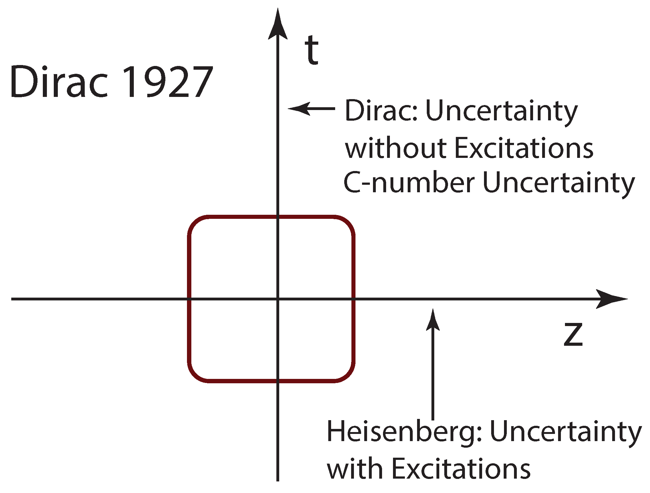
Dirac noted, in 1927 [19], that the emission of photons from atoms is a manifestation of the uncertainty relation between the time and energy variables. He also noted that, unlike the uncertainty relation of Heisenberg which allows quantum excitations, the time or energy axis has no excitations along it. Hence, when attempting to combine these two uncertainty relations in the Lorentz-covariant world, there remains the serious difficulty that the space and time variables are linearly mixed.
Subsequently in 1945 [20], Dirac, using the four-dimensional harmonic oscillator attempted to construct, using the oscillator wave functions, a representation of the Lorentz group. When he did this, however, the wave functions which resulted did not appear to be Lorentz-covariant.
Using the ten generators of the inhomogeneous Lorentz group Dirac in 1949 [21], constructed from them three forms of relativistic dynamics. However, after imposing subsidiary conditions necessitated by the existing form of quantum mechanics, he found inconsistencies in all three of the forms he considered.
In 1963 [22], Dirac constructed a representation of the de Sitter group. To accomplish this, he used two coupled harmonic oscillators in the form of step-up and step-down operators. Thus Dirac constructed a beautiful algebra. He did not, however, attempt to exploit the physical contents of his algebra.
In spite of the shortcomings mentioned above, it is indeed remarkable that Dirac worked so tirelessly on this important subject. We are interested in combining all of his works to achieve his goal of making quantum mechanics consistent with special relativity. Let us review the contents of these papers in detail, by transforming Dirac’s formulae into geometrical figures.
2.1. Dirac’s C-Number Time-Energy Uncertainty Relation
It was Wigner who in 1972 [30] drew attention to the fact that the time-energy uncertainty relation, known from the transition time and line broadening in atomic spectroscopy, existed before 1927. This occurred even before the uncertainty principle that Heisenberg formulated in 1927. Also in 1927 [19], Dirac studied the uncertainty relation which was applicable to the time and energy variables. When the uncertainty relation was formulated by Heisenberg, Dirac considered the possibility of whether a Lorentz-covariant uncertainty relation could be formed out of the two uncertainty relations [19].
Dirac then noted that the time variable is a c-number and thus there are no excitations along the time-like direction. However, there are excitations along the space-like longitudinal direction starting from the position-momentum uncertainty. Since the space and time coordinates are mixed up for moving observers, Dirac wondered how this space-time asymmetry could be made consistent with Lorentz covariance. This was indeed a major difficulty.
Dirac, however, never addressed, even in his later papers, the separation in time variable or the time interval. On the other hand, the Bohr radius, which measures the distance between the proton and electron is an example of Heisenberg’s uncertainty relation, applicable to space separation variables.
In his 1949 paper [21] Dirac discusses his instant form of relativistic dynamics. Thus Dirac came back to this question of the space-time asymmetry, in his 1949 paper. There he addresses indirectly the possibility of freezing three of the six parameters of the Lorentz group, and hence only working with the remaining three parameters. Wigner, in this 1939 paper [2,13] already presented this idea. He had observed in that paper that his little groups with three independent parameters dictated the internal space-time symmetries of particles.
2.2. Dirac’s Four-Dimensional Oscillators
Since the language of special relativity is the Lorentz group, and harmonic oscillators provide a start for the present form of quantum mechanics, Dirac, during the second World War, considered the possibility of using harmonic oscillator wave functions to construct representations of the Lorentz group [20]. He considered that, by constructing representations of the Lorentz group using harmonic oscillators, he might be able to make quantum mechanics Lorentz-covariant.
Thus in his 1945 paper [20], Dirac considers the Gaussian form
The x and y variables can be dropped from this expression, as we are considering a Lorentz boost only along the z direction. Therefore we can write the above equation as:
Since is an invariant quantity, the above expression may seem strange for those who believe in Lorentz invariance.
In his 1927 paper [19] Dirac proposed the time-energy uncertainty relation, but observed that. because time is a c-number, there are no excitations along the time axis. Hence the above expression is consistent with this earlier paper.
If we look carefully at Figure 1, we see that this figure is a pictorial illustration of Dirac’s Equation (2). There is localization in both space and time coordinates. Dirac’s fundamental question, illustrated in Figure 2, would then be how to make this figure covariant. Dirac stops there. However, this is not the end of his story.
2.3. Dirac’s Light-Cone Coordinate System
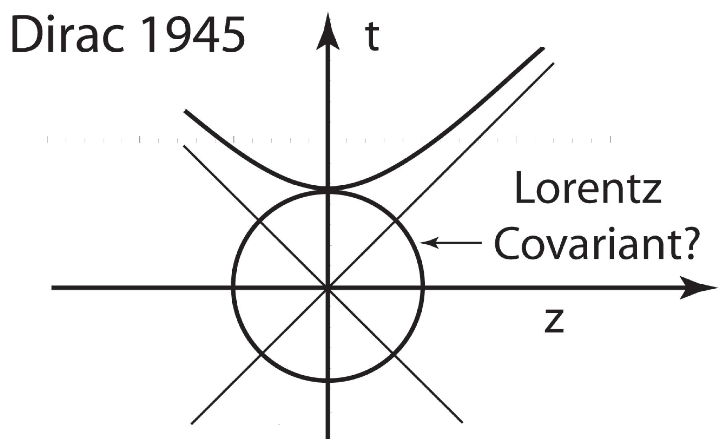
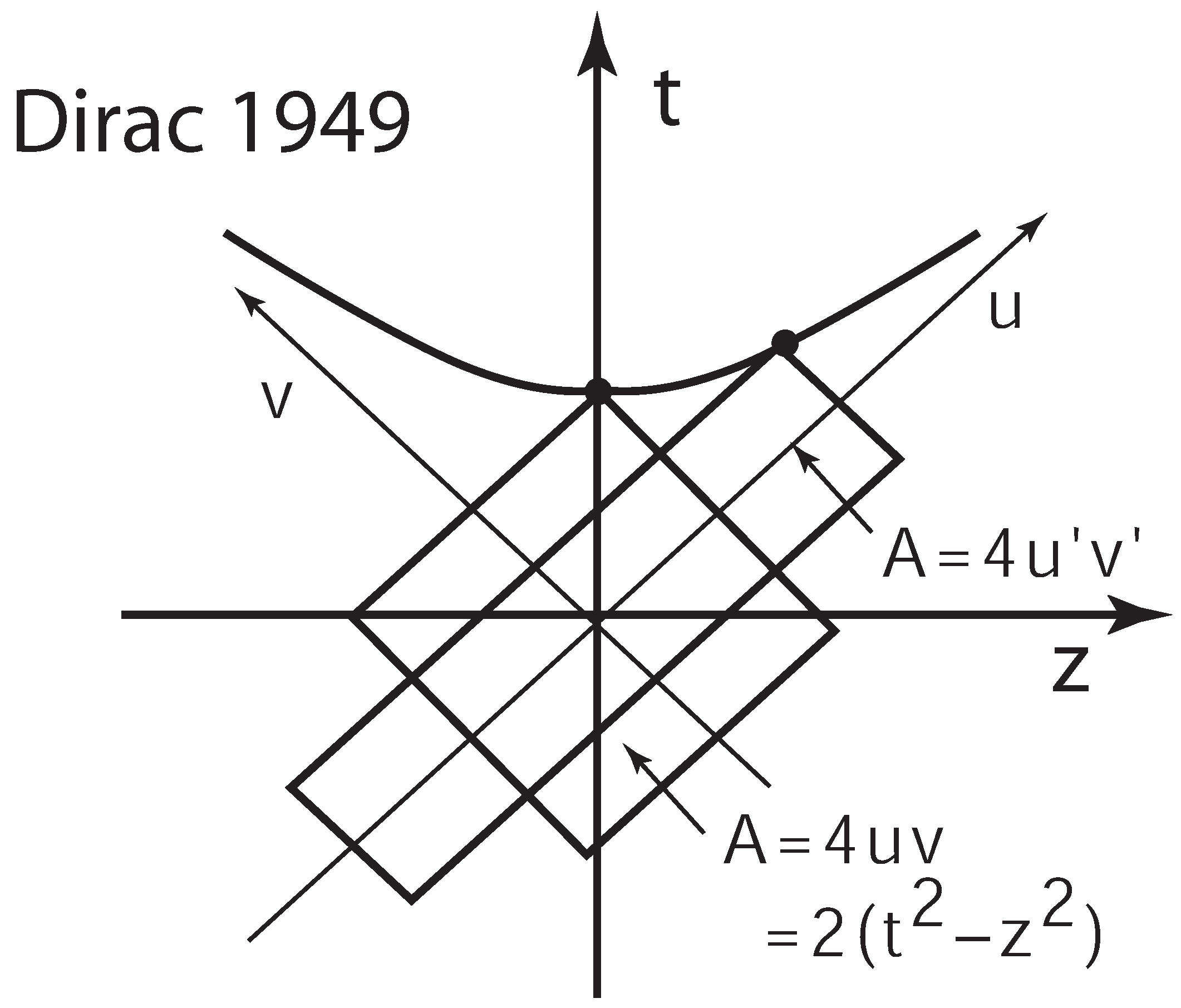
The Reviews of Modern Physics, in 1949, celebrated Einstein’s 70th birthday by publishing a special issue. In this issue was included Dirac’s paper entitled Forms of Relativistic Dynamics [21]. Here Dirac introduced his light-cone coordinate system. In this system a Lorentz boost is seen to be a squeeze transformation, where one axis expands while the other contracts in such a way that their product remains invariant as shown in Figure 3.
When boosted along the z direction, the system is transformed into the following form:
Dirac defined his light-cone variables as [21]
Then the form of the boost transformation of Equation (3) becomes
It is then apparent that u variable becomes expanded, but the v variable becomes contracted. We illustrate this in Figure 3. The product then becomes:
which remains invariant. The Lorentz boost is therefore, in Dirac’s picture, a squeeze transformation.
Dirac also introduced his 1949 paper his instant form of relativistic quantum mechanics. This has the condition
What did his approximate equality mean? In this paper, we interpret the nature of the time-energy uncertainty relation in terms of his c-number. Furthermore, it could mean that it is, for the massive particle is the three-dimensional rotation group, Wigner’s little group, without the time-like direction.
Additionally, Dirac stated that constructing a representation of the inhomogeneous Lorentz group, was necessary to construct a relativistic quantum mechanics. The inhomogeneous Lorentz group has ten generators, four space-time translation generators, three rotation generators, and three boost generators, which satisfy a closed set of commutation relations.
It is now clear that Dirac was interested in using harmonic oscillators to construct a representation of the inhomogeneous Lorentz group. In 1979, together with another author, the present authors published a paper on this oscillator-based representation [12]. We regret that we did not mention there Dirac’s earlier efforts along this line.
3. Scattering and Bound States
From the three papers written by Dirac [19,20,21], let us find out what he really had in mind. In physical systems, there are scattering and bound states. Throughout his papers, Dirac did not say he was mainly interested in localized bound systems. Let us clarify this issue using the formalism of Feynman, Kislinger, and Ravndal [25].
We are quite familiar with the Klein–Gordon equation for a free particle in the Lorentz-covariant world. We shall use the four-vector notations
Then the Klein–Gordon equation becomes
The solution of this equation takes the familiar form
In 1971, Feynman et al. [25] considered two particles a and b bound together by a harmonic oscillator potential, and wrote down the equation
The bound state of these two particles is one hadron. The constituent particles are called quarks. We can then define the four-coordinate vector of the hadron as
and the space-time separation four-vector between the quarks as
Then Equation (11) becomes
This differential equation can then be separated into
with
where and satisfy their own equations:
and
Here, the wave function then takes the form
where are for the hadronic momentum, and
Here the hadronic mass M is determined by the parameter , which is the eigenvalue of the differential equation for given in Equation (18).
Considering Feynman diagrams based on the S-matrix formalism, quantum field theory has been quite successful. It is, however, only useful for physical processes where, after interaction, one set of free particles becomes another set of free particles. The questions of localized probability distributions and their covariance under Lorentz transformations is not addressed by quantum field theory. In order to tackle this problem and address these questions, Feynman et al. suggested harmonic oscillators [25]. In Figure 4, we illustrate this idea.
However, for their wave function , Feynman et al. uses a Lorentz-invariant exponential form
This wave function increases as t becomes large. This is not an acceptable wave function. They overlooked the normalizable exponential form given by Dirac in Equation (1). They also overlooked the form in the paper of Fujimura et al. [31] which was quoted in their own paper.
Thus, we are interested in fixing this problem and thus constructing Lorentz-covariant oscillator wave functions satisfying both the rules of quantum mechanics and the rules of special relativity.
4. Lorentz-Covariant Picture of Quantum Bound States
In 1939, Wigner considered internal space-time symmetries of particles in the Lorentz-covariant world [13]. For this purpose, he considered the subgroups of the Lorentz group for a given four-momentum of the particle. For the massive particle, the internal space-time symmetry is defined for when the particle is at rest, and its symmetry is dictated by the three-dimensional rotation group, which allows us to define the particle spin as a dynamical variable, as indicated in Table 1.
Let us go to the wave function of Equation (19). This wave function is for the internal coordinates of the hadron, and the exponential form defines the hadron momentum. Thus, the symmetry of Wigner’s little group is applicable to the wave function .
This situation is like the case of the Dirac equation for a free particle. Its solution is a plane wave times the four-component Dirac spinor describing the spin orientation and its Lorentz covariance. This separation of variables for the present case of relativistic extended particles is illustrated in Figure 4. With this understanding let us write the Lorentz-invariant differential equation as
Here, the variables are for the spatial separation between the quarks, like the Bohr radius in the hydrogen atom. The time variable t is the time separation between the quarks. This variable is very strange, because it does not exist in the present forms of quantum mechanics and quantum field theory. Paul A. M. Dirac did not mention this time separation in any of his papers quoted here. Yet, it plays the major role in the Lorentz-covariant world, because the spatial separation (like the Bohr radius) picks up a time-like component when the system is Lorentz-boosted [32].
In his 1927 paper [19], Dirac mentioned the c-number time-energy uncertainty relation, and he used in his 1949 paper for his instant form of relativistic dynamics. When he wrote down a Gaussian function with as the exponent, he should have meant and z are for the space separation and t for the time separation, since otherwise the system becomes zero in the remote future and remote past.
With this understanding, we are dealing here with the solution of the differential equation of the form
where satisfy the oscillator differential equation
The form of Equation (23) tells us there are no time-like excitations. This equation is the Schrödinger equation for the three-dimensional harmonic oscillator and its solutions are well known.
If we use the three-dimensional spherical coordinate system, the solution will give the spin or internal angular momentum and the orientation of the bound-state hadron [12]. This spherical form is for the symmetry of Wigner’s little group for massive particles. The Lorentz-invariant Casimir operators are given in Ref. [12].
If we are interested in Lorentz-boosting the wave function, we note that the original wave equation of Equation (22) is separable in all four variables. If the Lorentz boost is made along the z direction, the wave functions along the x and y directions remain invariant, and thus can be separated. We can study only the longitudinal and time-like components. Thus the differential equation of Equation (22) is reduced to
The solution of this differential equation takes the form
where is the Hermite polynomial. There are no excitations in t, therefore it is restricted to the ground state. For simplicity, we ignore the normalization constant.
If this wave function is Lorentz-boosted along the z direction, the z and t variables in this expression should be replaced according to
According to the light-cone coordinate system introduced by Dirac in 1949 [20], this transformation can be written as
Thus the Lorentz-boosted wave function becomes
without the normalization constant.
It is possible to write this wave function using the one-dimensional normalized oscillator functions and as
The most interesting case is the expansion of the ground state. The normalized wave function is then
The Lorentz-boost property of this form is illustrated in Figure 5. The expansion in the harmonic oscillator wave functions takes the form
This expression is the key formula for two-photon coherent states or squeezed states of light [14]. We shall return to this two-photon problem in Section 6.
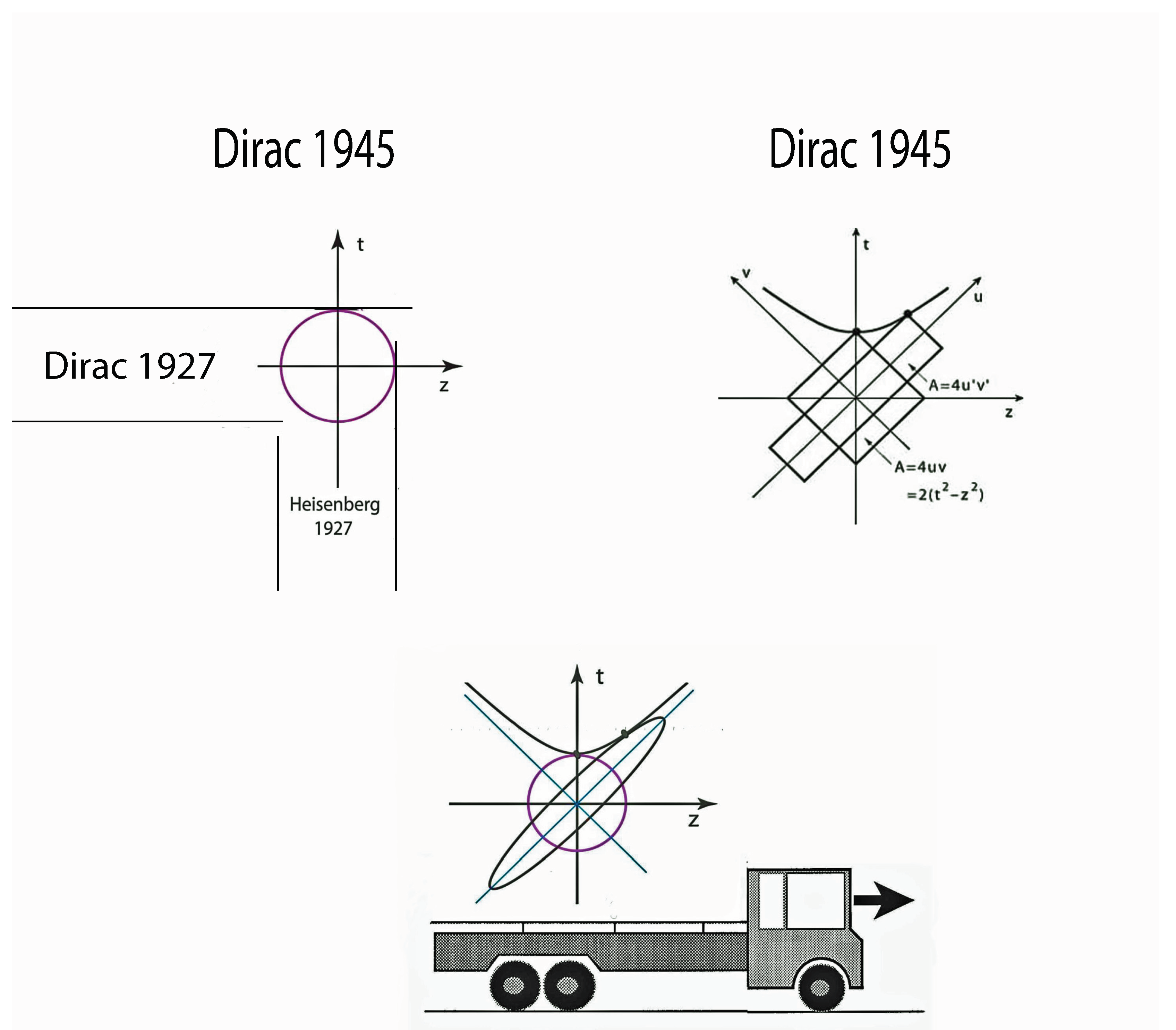
As for the wave function , this is the localized wave function Dirac was considering in his papers of 1927 and 1945. If Figure 2 and Figure 3 are combined, we end up with an ellipse as a squeezed circle as shown in Figure 5.
Indeed, one of the most controversial issues in high-energy physics is explained by this squeezed circle. The bound-state quantum mechanics of protons, which are known to be bound states of quarks, are often assumed to be the same as that of the hydrogen atom. Then how would the proton look to an observer on a train becomes the question. According to Feynman [9,27], when the speed of the train becomes close to that of light, the proton appears like a collection of partons. However, the properties of Feynman’s partons are quite different from the properties of the quarks. This issue shall be discussed in more detail in Section 5.
5. Lorentz-Covariant Quark Model
Early successes in the quark model include the calculation of the ratio of the neutron and proton magnetic moments [34], and the hadronic mass spectra [25,35]. These are based on hadrons at rest. We are interested in this paper how the hadrons in the quark model appear to observers in different Lorentz frames.
These days, modern particle accelerators routinely produce protons moving with speeds very close to that of light. Thus, the question is therefore whether the covariant wave function developed in Section 4 can explain the observed phenomena associated with those protons moving with relativistic speed.
The idea that the proton or neutron has a space-time extension had been developed long before Gell-Mann’s proposal for the quark model [8]. Yukawa [36] developed this idea as early as 1953, and his idea was followed up by Markov [37], and by Ginzburg and Man’ko [38].
Since Einstein formulated his special relativity for point particles, it has been and still is a challenge to formulate a theory for particles with space-time extensions. The most naive idea would be to study rigid spherical objects, and there were many papers on this subjects. But we do not know where that story stands these days. We can however replace these extended rigid bodies by extended wave packets or standing waves, thus by localized probability entities. Then what are the constituents within those localized waves? The quark model gives the natural answer to this question.
Hofstadter and McAllister [39], by using electron-proton scattering to measure the charge distribution inside the proton, made the first experimental discovery of the non-zero size of the proton. If the proton were a point particle, the scattering amplitude would just be a Rutherford formula. However, Hofstadter and MacAllister found a tangible departure from this formula which can only be explained by a spread-out charge distribution inside the proton.
In this section, we are interested in how well the bound-state picture developed in Section 4 works in explaining relativistic phenomena of those protons. In Section 5.1 we study in detail how the Lorentz squeeze discussed in Section 4 can explain the behavior of electron-proton scattering as the momentum transfer becomes relativistic.
Second, we note that the proton is regarded as a bound state of the quarks sharing the same bound-state quantum mechanics with the hydrogen atom. However, it appears as a collection of Feynman’s partons. Thus, it is a great challenge to see whether one Lorentz-covariant formula can explain both the static and light-like protons. We shall discuss this issue in Section 5.2.
One hundred years ago, Einstein and Bohr met occasionally to discuss physics. Bohr was interested in how the election orbit looks and Einstein was worrying about how things look to moving observers. Did they ever talk about how the hydrogen atom appears to moving observers? In Section 5.3, we briefly discuss this issue.
It is possible to conclude from the previous discussion that the Lorentz boost might increase the uncertainty. To deal with this, in Section 5.4, we address the issue of the uncertainty relation when the oscillator wave functions are Lorentz-boosted.
5.1. Proton Form Factor
Using the Born approximation for non-relativistic scattering, we see what effect the charge distribution has on the scattering amplitude. When electrons are scattered from a fixed charge distribution with a density of , the scattering amplitude becomes:
Here we use and which is the momentum transfer. We can reduce this amplitude to:
The density function’s Fourier transform is given by which can be written as:
This above quantity is called the form factor and it describes the charge distribution in terms of the momentum transfer which can be normalized by:
Therefore, from Equation (35), F(0) = 1. the scattering amplitude of Equation (33) becomes the Rutherford formula for Coulomb scattering if the density function, corresponding to a point charge, is a delta function, , for all values of . Increasing values of , which are deviations from Rutherford scattering, give a measure of the charge distribution. Hofstadter’s experiment, which scattered electrons from a proton target, found this precisely [39].
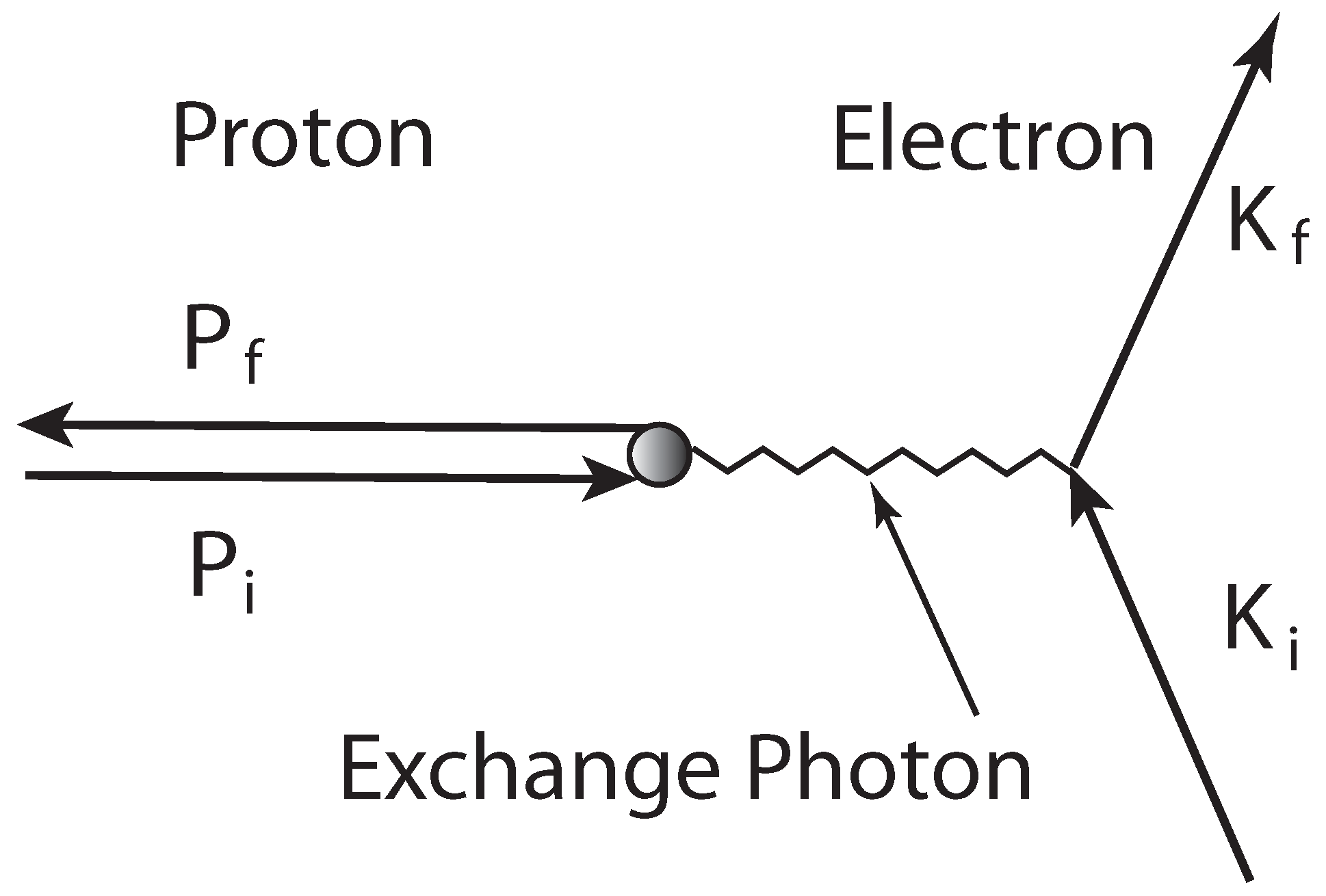
When the energy of the incoming electron becomes higher, it is necessary to take into account the recoil effect of target proton. It then requires that the problem be formulated in the Lorentz-covariant framework. It is generally agreed that quantum electrodynamics can describe electrons and their electromagnetic interaction by using Feynman diagrams for practical calculations. When using perturbation, a power series of the fine structure constant is used to expand the scattering amplitude. Therefore, the lowest order in can, using the diagram given in Figure 6, describe the scattering of an electron by a proton.
Many textbooks on elementary particle physics [40,41] give the corresponding matrix element as the form:
where the initial and final four-momenta of the proton and electron, respectively, are given by and . The Dirac spinor for the initial proton is , while the (four-momentum transfer, , is
If the proton were a point particle like the electron, the would be , but for a particle, like the proton, with space-time extension, it is . The virtual photon being exchanged between the electron and the proton produces the factor in Equation (37). For the particles involved in the scattering process this quantity is positive for physical values of the four-momenta in the metric we use.
From the definition of the form factor given in Equation (35), we can make a relativistic calculation of the form factor. The density function, which depends only on the target particle, is proportional to . The wave function for quarks inside the proton is . This expression is a special case of the more general form
where the initial and final wave function of the target atom is given by and . The form factor of Equation (35) can then be written as
The required Lorentz generalization, starting from this expression, can be made using the relativistic wave functions for hadrons.
By replacing each quantity in the expression of Equation (35) by its relativistic counterpart we should be able to see the details of the transition to relativistic physics. If we go back to the Lorentz frame in which the momenta of the incoming and outgoing nucleons have equal magnitude but opposite signs, we obtain
This kinematical condition is illustrated in Figure 6.
We call the Lorentz frame in which the above condition holds the Breit frame. As illustrated in Figure 6, there is no loss of generality if the proton comes in along the z direction before the collision and goes out along the negative z direction after the scattering process. The four vector, , ín this frame, has no time-like component. The Lorentz-invariant form, , can thus replace the exponential factor . The covariant harmonic oscillator wave functions discussed in this paper can be used for the wave functions for the protons, assuming that the nucleons are in the ground state. Then the integral in the evaluation of Equation (35), which includes the time-like direction and is thus four-dimensional, is the only difference between the non-relativistic and relativistic cases. The exponential factor, which does not depend on the time-separation variable, therefore, is not affected by the integral in the time-separation variable.
We can now consider the integral:
where is the velocity parameter () for the incoming proton, and the wave function , from Equation (31), takes the form:
We can, now, after the above decomposition of the wave functions, perform the integrations in the x and y variables trivially. We can, after dropping these trivial factors, write the product of the two wave functions as
Now the z and t variables are separated. Since the t integral in Equation (42), as the exponential factor in Equation (35), does not depend on t, it can also be trivially performed. Then integral of Equation (42) can be written as
Here the z component of the momentum of the incoming proton is P. The variable , which is the (momentum transfer, now become . The hadronic material, which is distributed along the longitudinal direction, has indeed became contracted [42].
We note that can be written as
where M is the proton mass. This equation tells us that when , while it becomes one as becomes infinity.
The evaluation of the above integral for in Equation (45) leads to
For the above expression becomes 1. It decreases as
as assumes large values.
So far the calculation has been performed for an oscillator bound state of two quarks. The proton, however, consists of three quarks. As shown in the paper of Feynman et al. [25], the problem becomes a product of two oscillator modes. Thus, the three-quark system is a straightforward generalization of the above calculation. As a result, the form factor becomes;
which is 1 at , and decreases as
as assumes large values. This form factor function has the required dipole-cut-off behavior, which has been observed in high-energy laboratories. This calculation was carried first by Fujimura et al. in 1970 [31].
Let us re-examine the above calculation. If we replace by zero in Equation (45) and ignore the elliptic deformation of the wave functions, will become
which will lead to an exponential cut-off of the form factor. This is not what we observe in laboratories.
In order to gain a deeper understanding of the above-mentioned correlation, let us study the case using the momentum-energy wave functions:
If we ignore, as before, the transverse components, we can write as [2]
The above overlap integral has been sketched in Figure 7. The two wave functions overlap completely in the plane if or . The wave functions become separated when P increases. Because of the elliptic or squeeze deformation, seen in Figure 7, they maintain a small overlapping region. In the non-relativistic case, there is no overlapping region, because the deformation is not taken into account, as seen in Figure 7. The slower decrease in is, therefore, more precisely given in the relativistic calculation than in the non-relativistic calculation.
Although our interest has been in the space-time behavior of the hadronic wave function, it must be noted that quarks are spin-1/2 particles. This fact must be taken into consideration. This spin effect manifests itself prominently in the baryonic mass spectra. Here we are concerned with the relativistic effects, therefore, it is necessary to construct a relativistic spin wave function for the quarks. The result of this relativistic spin wave function construction for the quark wave function should be a hadronic spin wave function. In the case of nucleons, the quark spins should be combined in a manner to generate the form factor of Equation (44).
Naively we could use free Dirac spinors for the quarks. However, it was shown by Lipes [43] that using free-particle Dirac spinors leads to a wrong behavior of the form factor. Lipes’ result, however, does not cause us any worry, as quarks in a hadron are not free particles. Thus we have to find suitable mechanism in which quark spins, coupled to orbital motion, are taken into account. This is a difficult problem and is a nontrivial research problem, and further study is needed along this direction [44].
In 1960, Frazer and Fulco calculated the form factor using the technique of dispersion relations [26]. In so doing they had to assume the existence of the so-called meson, which was later found experimentally, and which subsequently played a pivotal role in the development of the quark model.
Even these days, the form factor calculation occupies a very important place in recent theoretical models, such as quantum chromodynamics (QCD) lattice theory [45] and the Faddeev equation [46]. However, it is still noteworthy that Dirac’s form of Lorentz-covariant bound states leads to the essential dipole cut-off behavior of the proton form factor.
5.2. Feynman’S Parton Picture
As we did in Section 5.1, we continue using the Gaussian form for the wave function of the proton. If the proton is at rest, the z and t variables are separable, and the time-separation can be ignored, as we do in non-relativistic quantum mechanics. If the proton moves with a relativistic speed, the wave function is squeezed as described in Figure 5. If the speed reaches that of light, the wave function becomes concentrated along positive light cone with . The question then is whether this property can explain the parton picture of Feynman when a proton moves with a speed close to that of light.
It was Feynman who, in 1969, observed that a fast-moving proton can be regarded as a collection of many partons. The properties of these partons appear to be quite different from those of the quarks [2,9,27]. For example, while the number of quarks inside a static proton is three, the number of partons appears to be infinite in a rapidly moving proton. The following systematic observations were made by Feynman:
- When protons move with velocity close to that of light, the parton picture is valid.
- Partons behave as free independent particles when the interaction time between the quarks becomes dilated.
- Partons have a widespread distribution of momentum as the proton moves quickly.
- There seems to be an infinite number of partons or a number much larger than that of quarks.
The question is whether the Lorentz-squeezed wave function produced in Figure 5 can explain all of these peculiarities.
Each of the above phenomena appears as a paradox, when the proton is believed to be a bound state of the quarks. This is especially true of (b) and (c) together. We can ask how a free particle can have a wide-spread momentum distribution.
To resolve this paradox, we construct the momentum-energy wave function corresponding to Equation (31). We can construct two independent four-momentum variables [25] if the quarks have the four-momenta and .
Since P is the total four-momentum, it is the four-momentum of the proton. The four-momentum separation between the quarks is measured by q. We can then write the light-cone variables as
This results in the momentum-energy wave function
Since the harmonic oscillator is being used here, it is easily seen that the above momentum-energy wave function has the identical mathematical form to that of the space-time wave function of Equation (31) and that these wave functions also have the same Lorentz squeeze properties. Though discussed extensively in the literature [2,10,11], these mathematical forms and Lorentz squeeze properties are illustrated again in Figure 8 of the present paper.
We can see from the figure, that both wave functions behave like those for the static bound state of quarks when the proton is at rest with . However, it can also be seen that as increases, the wave functions become concentrated along their respective positive light-cone axes as they become continuously squeezed. If we look at the z-axis projection of the space-time wave function, we see that, as the proton speed approaches that of the speed of light, the width of the quark distribution increases. Thus, to the observer in the laboratory, the position of each quark appears widespread. Thus the quarks appear like free particles.
If we look at the momentum-energy wave function we see that it is just like the space-time wave function. As the proton speed approaches that of light, the longitudinal momentum distribution becomes wide-spread. In non-relativistic quantum mechanics we expect that the width of the momentum distribution is inversely proportional to that of the position wave function. This wide-spread longitudinal momentum distribution thus contradicts our expectation from non-relativistic quantum mechanics. Our expectation is that free quarks must have a sharply defined momenta, not a wide-spread momentum distribution.
However, as the proton is boosted, the space-time width and the momentum-energy width increase in the same direction. This is because of our Lorentz-squeezed space-time and momentum-energy wave functions. If we look at Figure 5 and Figure 8 we see that is the effect of Lorentz covariance described in these figures. One of the quark-parton puzzles is thus resolved [2,10,11].
Another puzzling problem is that quarks are coherent when the proton is at rest but the partons appear as incoherent particles. We could ask whether this means that Lorentz boost coherence is destroyed. Obviously, the answer to this question is NO. The resolution to this puzzle is given below.
When the proton is boosted, its matter becomes squeezed. The result is that the wave function for the proton becomes, along the positive light-cone axis, concentrated in the elliptic region. The major axis is expanded in length by , and, as a consequence, the minor axis is contracted by .
Therefore we see that, among themselves, the interaction time of the quarks becomes dilated. As the wave function becomes wide-spread, the ends of the harmonic oscillator well increase in distance from each other. Universally observed in high-energy experiments, it was Feynman [9] who first observed this effect. The oscillation period thus increase like [27,47].
Since the external signal, on the other hand, is moving in the direction opposite to the direction of the proton, it travels along the negative light-cone axis with . As the proton contracts along the negative light-cone axis, the interaction time decreases by . Then the ratio of the interaction time to the oscillator period becomes . Each proton, produced by the Fermilab accelerator, used to have an energy of . This then means the ratio is . Because this is such small number, the external signal cannot sense, inside the proton, the interaction of the quarks among themselves.
5.3. Historical Note
The hydrogen atom played a pivotal role in the development of quantum mechanics. Niels Bohr devoted much of his life to understanding the electron orbit of the hydrogen atom. Bohr met Einstein occasionally to talk about physics. Einstein’s main interest was how things look to moving observers. Then, did they discuss how the hydrogen atom looks to a moving observer?
If they discussed this problem, there are no records. If they did not, they are excused. At their time, the hydrogen atom moving with a relativistic speed was not observable, and thus beyond the limit of their scope. Even these days, this atom with total charge zero cannot be accelerated.
After 1950, high-energy accelerators started producing protons moving with relativistic speeds. However, the proton is not a hydrogen atom. On the other hand, Hofstadter’s experiment [39] showed that the proton is not a point particle. In 1964, Gell-Mann produced the idea that the proton is a bound-state of more fundamental particles called quarks. It is assumed that the proton and the hydrogen share the same quantum mechanics in binding their constituent particles. Thus, we can study the moving hydrogen atom by studying the moving proton. This historical approach is illustrated in Figure 9.
Paul A. M. Dirac was interested in constructing localized wave functions that can be Lorentz boosted. He wrote three papers [19,20,21]. If we integrate his ideas, it is possible to construct the covariant oscillator wave function discussed in this paper. Figure 10 tells where this integration stands in the history of physics.
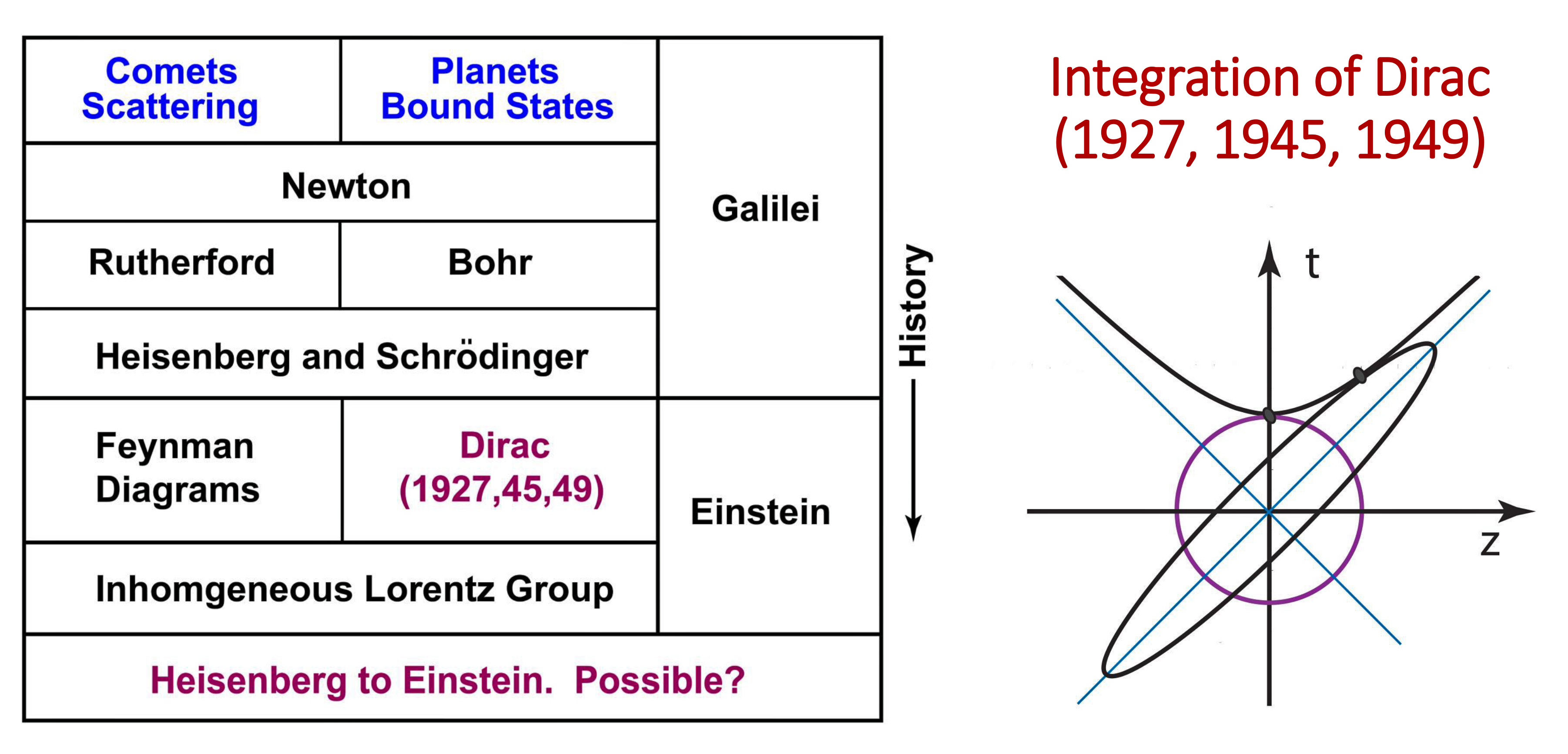
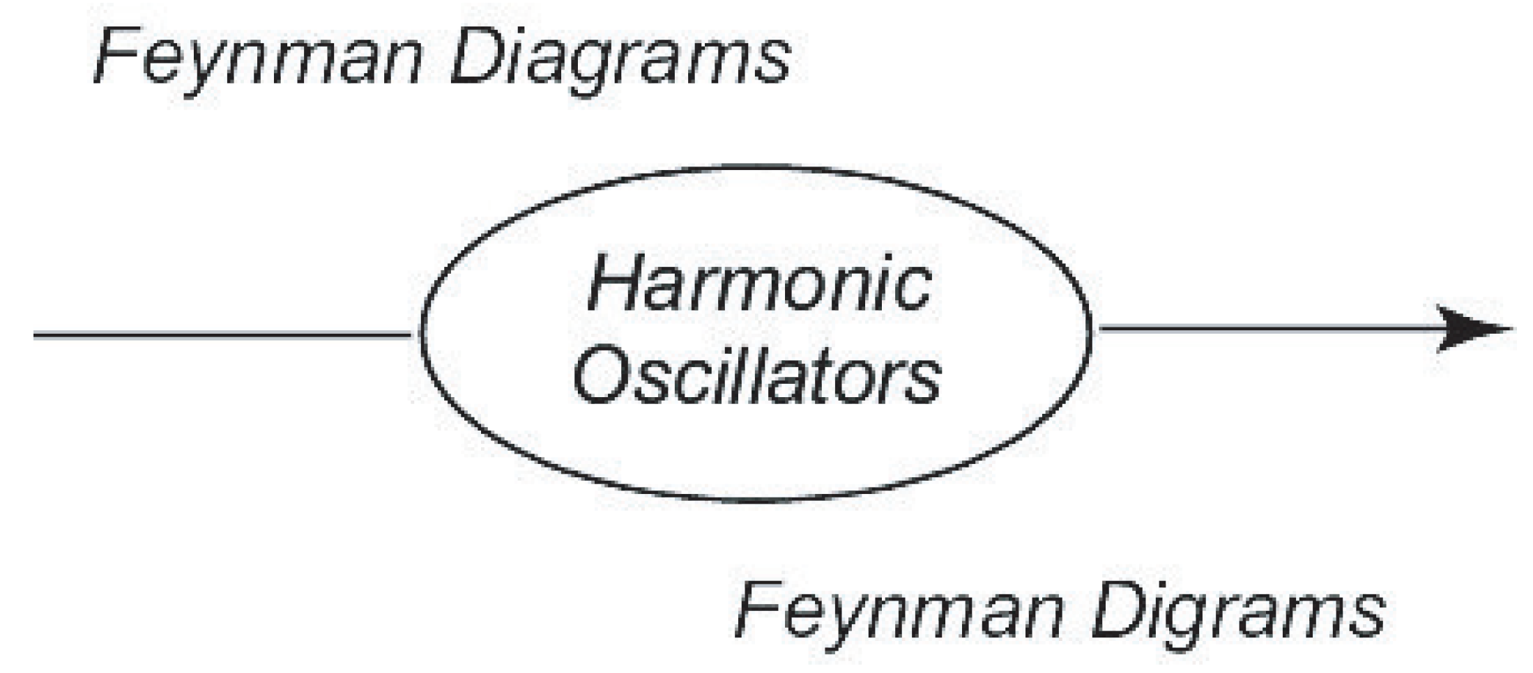
In constructing quantum mechanics in the Lorentz-covariant world, the present form of quantum field theory is quite successful in scattering problems where all participating particles are free in the remote past and the remote future. The bound states are different, and Feynman suggested Lorentz-covariant harmonic oscillators for studying this problem [25]. Yes, quantum field theory and the covariant harmonic oscillators use quite different mathematical forms. Yet, they share the same set of physical principles [48]. They are both the representations of the inhomogeneous Lorentz group. We note that Dirac in his 1949 paper [21] said that we can build relativistic dynamics by constructing representations of the inhomogeneous Lorentz group. In Figure 10, both Feynman diagrams and the covariant oscillator (integration of Dirac’s papers) share the Lie algebra of the inhomogeneous Lorentz group. This figure leads to the idea of whether the Lie algebra of quantum mechanics can lead to that of the inhomogeneous Lorentz group. We shall discuss this question in Section 7.
Since the time of Bohr and Einstein, attempts have been made to construct Lorentz-covariant bound states within the framework of quantum mechanics and special relativity. In recent years, there have been laudable efforts to construct a non-perturbative approach to quantum field theory, where particles are in a bound state and thus are not free in the remote past and remote future [49]. If and when this approach produces localized probability distributions which can Lorentz-boosted, it should explain both the quark model (at rest) and its parton picture in the limit of large speed.
In recent years, there have been efforts to represent the observation of movements inside materials using Dirac electric states [50] as well as to use relativistic methods to understand atomic and molecular structure [51]. There have also been efforts to provide covariant formulation of the electrodynamics of nonlinear media [52].
5.4. Lorentz-Invariant Uncertainty Products
In the harmonic oscillator regime, the energy-momentum wave functions take the same mathematical form, and the uncertainty relation in terms of the uncertainty products is well understood. However, in the present case, the oscillator wave functions are deformed when Lorentz-boosted, as shown in Figure 8. According to this figure, both the space-time and momentum-energy wave functions become spread along their longitudinal directions. Does this mean that the Lorentz boost increases the uncertainty?
In order to address this question, let us write the momentum-energy wave function as a Fourier transformation of the space-time wave function:
The transverse x and y components are not included in this expression. The exponent of this expression can be written as
with
as given earlier in Equations (4) and (55).
In terms of these variables, the Fourier integral takes the form
In this case, the variable is conjugate to , and to . Let us go back to Figure 8. The major (minor) axis of the space-time ellipse is conjugate to the minor (major) axis of the momentum-energy ellipse. Thus the uncertainty products
remain invariant under the Lorentz boost.
6. O(3,2) Symmetry Derivable from Two-Photon States
In this section we start with the paper Dirac published in 1963 on the symmetries from two harmonic oscillators [22]. Since the step-up and step-down operators in the oscillator system are equivalent to the creation and annihilation operators in the system of photons, Dirac was working with the system of two photons which is of current interest [5,53,54,55].
In the oscillator system the step-up and step-down operators are:
with
In terms of these operators, Heisenberg’s uncertainty relations can be written as
with
With these sets of operators, Dirac constructed three generators of the form
and three more of the form
These and operators satisfy the commutation relations
This set of commutation relations is identical to the Lie algebra of the Lorentz group where and are three rotation and three boost generators respectively. This set of commutators is the Lie algebra of the Lorentz group with three rotation and three boost generators.
In addition, with the harmonic oscillators, Dirac constructed another set consisting of
They then satisfy the commutation relations
Together with the relation given in Equation (68), and produce another Lie algebra of the Lorentz group. Like , the operators act as boost generators.
In order to construct a closed set of commutation relations for all the generators, Dirac introduced an additional operator
Then the commutation relations are
It was then noted by Dirac that the three sets of commutation relations given in Equations (68), (70) and (72) form the Lie algebra for the de Sitter group. This group applies to space of , which is five-dimensional. In this space, the three space-like coordinates are , and the time-like variables are given by t and s. Therefore, these generators are five-by-five matrices. The three rotation generators for the space-like coordinates are given in Table 2. The three boost generators with respect to the time variable t are given in Table 3. Table 4 contains three boost operators with respect to the second time variable s and the rotation generator between the two time variables t and s.
It is indeed remarkable, as Dirac stated in his paper [22], that the space-time symmetry of the (3 + 2) de Sitter group is the result of this two-oscillator system. What is even more remarkable is that we can derive, from quantum optics, this two-oscillator system. In the two-photon system in optics, where i can be 1 or 2, and act as the annihilation and creation operators.
It is possible to construct, with these two sets of operators, two-photon states [5]. Yuen, as early as 1976 [14], used the two-photon state generated by
This leads to the two-mode coherent state. This is also known as the squeezed state.
It was later that Yurke, McCall, and Klauder, in 1986 [56], investigated two-mode interferometers. In their study of two-mode states, they started with given in Equation (73). Then they considered that the following two additional operators,
were needed in one of their interferometers. These three Hermitian operators from Equations (73) and (74) have the following commutation relations
Yurke et al. called this device the interferometer. The group is isomorphic to the group or the Lorentz group applicable to two space-like and one time-like dimensions.
In addition, in the same paper [56], Yurke et al. discussed the possibility of constructing another interferometer exhibiting the symmetry generated by
These generators satisfy the closed set of commutation relations
given in Equation (66). This is the Lie algebra for the three-dimensional rotation group. Yurke et al. called this optical device the interferometer.
We are then led to ask whether it is possible to construct a closed set of commutation relations with the six Hermitian operators from Equations (75) and (76). It is not possible. We have to add four additional operators, namely
There are now ten operators. They are precisely those ten Dirac constructed in his paper of 1963 [22].
It is indeed remarkable that Dirac’s algebra is produced by modern optics. This algebra produces the Lorentz group applicable to three space-like and two time-like dimensions.
The algebra of harmonic oscillators given in Equation (64) is Heisenberg’s uncertainty relations in a two-dimensional space. The de Sitter group is basically a language of special relativity. Does this mean that Einstein’s special relativity can be derived from the Heisenberg brackets? We shall examine this problem in Section 7.
7. Contraction of O(3, 2) to the Inhomogeneous Lorentz Group
According to Section 6, the group has an subgroup with six generators plus four additional generators. The inhomogeneous Lorentz group also contains one Lorentz group as its subgroup plus four space-time translation generators. The question arises whether the four generators in Table 4 can be converted into the four translation generators. The purpose of this section is to prove this is possible according to the group contraction procedure introduced first by Inönü and Wigner [57].
In their paper Inönü and Wigner introduced the procedure for transforming the Lorentz group into the Galilei group. This procedure is known as group contraction [57]. In this section, we use the same procedure to contract the group into the inhomogeneous Lorentz group which is the group plus four translations.
Let us introduce the contraction matrix
This matrix expands the axes, and contracts s axis as becomes small. Yet, the and matrices given in Table 2 and Table 3 remain invariant:
These matrices have zero elements in the fifth row and fifth column.
On the other hand, the matrices in Table 4 are different. Let us choose . The same algebra leads to the elements and its inverse, as shown in this equation:
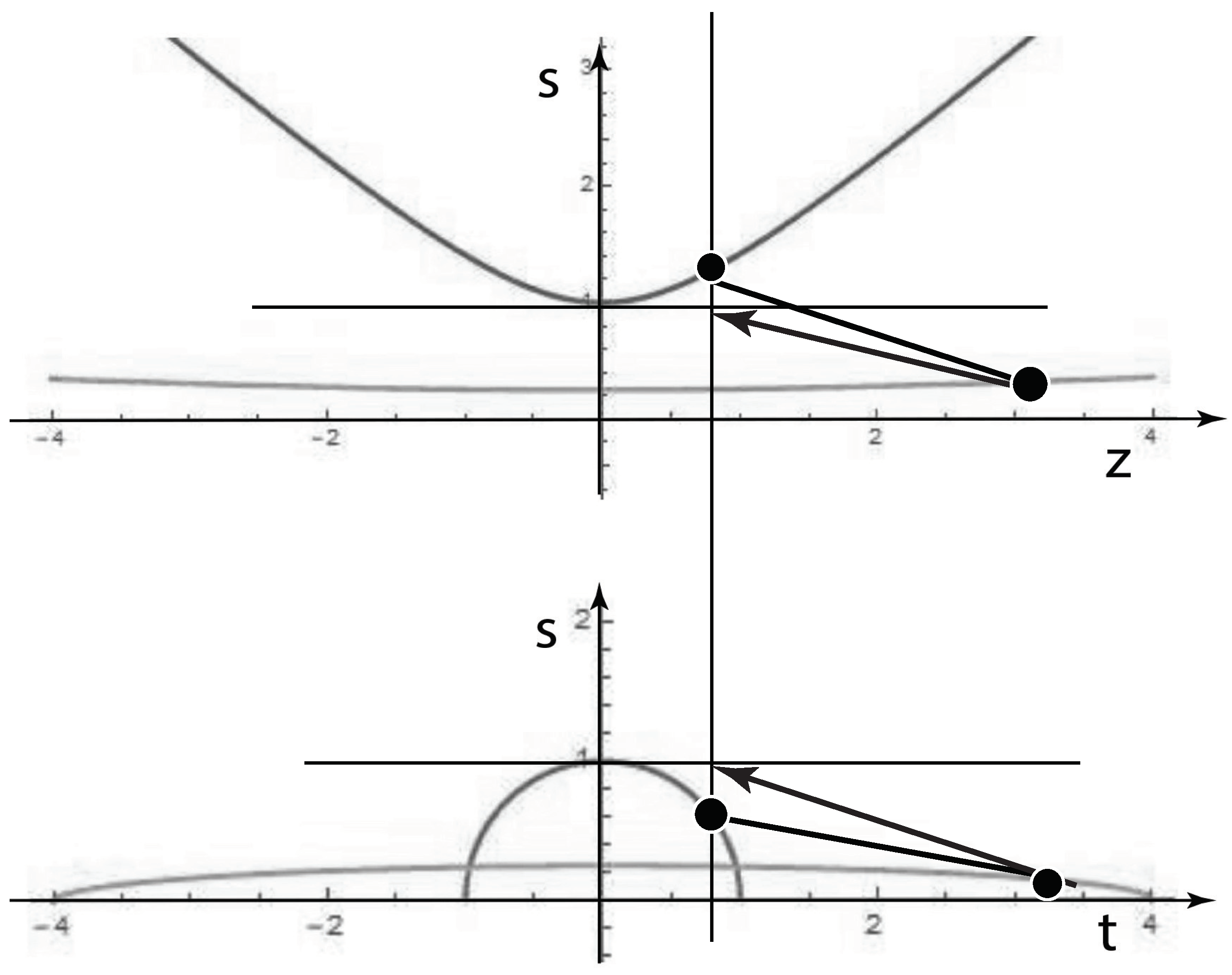
The second line of this equation tells us that becomes zero in the limit of small . If we make the inverse transformation, result is . We can perform the same algebra to arrive at the the results given in Table 5. According to this table, and become contracted to the generators of the space-time translations. In other words, the de Sitter group can be contracted to the inhomogeneous Lorentz group.
If this matrix is applied to the five-vector of , it becomes . If becomes very small, the s axis contracts while the four others expand. As becomes very small, approaches zero and can be replaced by , since both of them are zero. We are replacing zero by another zero, as shown here:
This contraction procedure is indicated in Figure 11.
Indeed, the five-vector serves as the space-time five-vector of the inhomogeneous Lorentz group. The transformation matrix applicable to this five-vector consists of that of the Lorentz group in its first four row and columns. Let us see how the generators and generate translations. First of all, in terms of these generators, the transformation matrix takes the form
If this matrix is applied to the five-vector , the result is the translation:
The five-by-five matrix of Equation (84) indeed performs the translations.
Let us go to Table 5 again. The four differential forms of the translation generators correspond to the four-momentum satisfying the equation . This is of course Einstein’s .
8. Concluding Remarks
Since 1973, the present authors have been publishing papers on the harmonic oscillator wave functions which can be Lorentz-boosted. The covariant harmonic oscillator plays roles in understanding some of the properties in high-energy particle physics. This covariant oscillator can also be used as a representation of Wigner’s little group for massive particles.
More recently, the oscillator wave function was shown to provide basic mathematical tools for two-photon coherent states known as the squeezed state of light [5].
In this paper, we have provided a review of our past efforts, with the purpose of integrating the papers Paul A. M. Dirac wrote in his lifelong efforts to make quantum mechanics compatible with Einstein’s special relativity which produced the Lorentz-covariant energy-momentum relation. It is interesting to note that Einstein’s special relativity is derivable from Heisenberg’s expression of the uncertainty relation.
Author Contributions
Both of the authors participated in developing the material presented in this paper and in writing the manuscript. All authors have read and agreed to the published version of the manuscript.
Funding
There is no extra funding for this paper.
Conflicts of Interest
The authors declare no conflict of interest.
References
- Kim, Y.S.; Noz, M.E. Covariant harmonic oscillators and the quark model. Phys. Rev. D 1973, 8, 3521–3627. [Google Scholar] [CrossRef]
- Kim, Y.S.; Noz, M.E. Theory and Applications of the Poincaré Group; Reidel: Dordrecht, The Netherlands, 1986. [Google Scholar]
- Başkal, S.; Kim, Y.S.; Noz, M.E. Physics of the Lorentz Group, IOP Concise Physics; Morgan & Claypool Publisher: San Rafael, CA, USA; IOP Publishing: Bristol, UK, 2015. [Google Scholar]
- Kim, Y.S.; Noz, M.E. New Perspectives on Einstein’s E = mc2; World Scientific: Singapore, 2018. [Google Scholar]
- Başkal, S.; Kim, Y.S.; Noz, M.E. Mathematical Devices for Optical Sciences; IOP Publishing: Bristol, UK, 2019. [Google Scholar]
- Ruiz, M.J. Orthogonality relations for covariant harmonic oscillator wave functions. Phys. Rev. D 1974, 10, 4306–4307. [Google Scholar] [CrossRef]
- Kim, Y.S.; Noz, M.E.; Oh, S.H. A simple method for illustrating the difference between the homogeneous and inhomogeneous Lorentz groups. Am. J. Phys. 1979, 47, 892–897. [Google Scholar] [CrossRef]
- Gell-Mann, M. A Schematic Model of Baryons and Mesons. Phys. Lett. 1964, 8, 214–215. [Google Scholar] [CrossRef]
- Feynman, R.P. Very High-Energy Collisions of Hadrons. Phys. Rev. Lett. 1969, 23, 1415–1417. [Google Scholar] [CrossRef] [Green Version]
- Kim, Y.S.; Noz, M.E. Covariant harmonic oscillators and the parton picture. Phys. Rev. D 1977, 15, 335–338. [Google Scholar] [CrossRef]
- Kim, Y.S. Observable gauge transformations in the parton picture. Phys. Rev. Lett. 1989, 63, 348–351. [Google Scholar] [CrossRef]
- Kim, Y.S.; Noz, M.E.; Oh, S.H. Representations of the Poincaré group for relativistic extended hadrons. J. Math. Phys. 1979, 20, 1341–1344. [Google Scholar] [CrossRef] [Green Version]
- Wigner, E. On unitary representations of the inhomogeneous Lorentz group. Ann. Math. 1939, 40, 149–204. [Google Scholar] [CrossRef]
- Yuen, H.P. Two-photon coherent states of the radiation field. Phys. Rev. A 1976, 13, 2226–2243. [Google Scholar] [CrossRef] [Green Version]
- Kim, Y.S.; Noz, M.E. Coupled oscillators, entangled oscillators, and Lorentz-covariant harmonic oscillators. J. Opt. B Quantum Semiclass. Opt. 2005, 7, S458–S467. [Google Scholar] [CrossRef]
- Başkal, S.; Kim, Y.S.; Noz, M.E. Harmonic Oscillators and Space Time Entanglement. Symmetry 2016, 8, 55. [Google Scholar] [CrossRef] [Green Version]
- Han, D.; Kim, Y.S.; Son, D. Gauge transformations as Lorentz-boosted rotations. Phys. Lett. B 1983, 131, 327–329. [Google Scholar] [CrossRef]
- Kim, Y.S.; Wigner, E.P. Space-time geometry of relativistic-particles. J. Math. Phys. 1990, 31, 55–60. [Google Scholar] [CrossRef]
- Dirac, P.A.M. The Quantum Theory of the Emission and Absorption of Radiation. Proc. R. Soc. (Lond.) 1927, A114, 243–265. [Google Scholar]
- Dirac, P.A.M. Unitary Representations of the Lorentz Group. Proc. R. Soc. (Lond.) 1945, A183, 284–295. [Google Scholar]
- Dirac, P.A.M. Forms of Relativistic Dynamics. Rev. Mod. Phys. 1949, 21, 392–399. [Google Scholar] [CrossRef] [Green Version]
- Dirac, P.A.M. A Remarkable Representation of the 3 + 2 de Sitter Group. J. Math. Phys. 1963, 4, 901–909. [Google Scholar] [CrossRef]
- Dirac, P.A.M. Can equations of motion be used in high energy physics? Phys. Today 1970, 23, 29–31. [Google Scholar] [CrossRef]
- Farmelo, G. The Strangest Man, the Hidden Life of Paul Dirac, Mystic of Atom; Basic Books: New York, NY, USA, 2009. [Google Scholar]
- Feynman, R.P.; Kislinger, M.; Ravndal, F. Current Matrix Elements from a Relativistic Quark Model. Phys. Rev. D 1971, 3, 2706–2732. [Google Scholar] [CrossRef] [Green Version]
- Frazer, W.; Fulco, J. Effect of a Pion-Pion Scattering Resonance on Nucleon Structure. Phys. Rev. Lett. 1960, 2, 365–368. [Google Scholar] [CrossRef] [Green Version]
- Bjorken, J.D.; Paschos, E.A. Electron-Proton and γ-Proton Scattering and the Structure of the Nucleon. Phys. Rev. 1969, 185, 1975–1982. [Google Scholar] [CrossRef]
- Başkal, S.; Kim, Y.S.; Noz, M.E. Poincaré Symmetry from Heisenberg’s Uncertainty Relations. Symmetry 2019, 11, 409. [Google Scholar] [CrossRef] [Green Version]
- Başkal, S.; Kim, Y.S.; Noz, M.E. Einstein’s E = mc2 derivable from Heisenberg’s Uncertainty Relations. Quantum Rep. 2019, 1, 236–251. [Google Scholar] [CrossRef] [Green Version]
- Wigner, E.P. On the Time-Energy Uncertainty Relation. In Aspects of Quantum Theory; Salam, A., Wigner, E.P., Eds.; Cambridge University Press: London, UK, 1972; pp. 237–247. [Google Scholar]
- Fujimura, K.; Kobayashi, T.; Namiki, M. Nucleon Electromagnetic Form Factors at High Momentum Transfers in an Extended Particle Model Based on the Quark Model. Prog. Theor. Phys. 1970, 43, 73–79. [Google Scholar] [CrossRef] [Green Version]
- Kim, Y.S.; Noz, M.E. The Question of Simultaneity in Relativity and Quantum Mechanics. In Quantum Theory: Reconsideration of Foundations–3; Adenier, G., Khrennikov, A., Nieuwenhuizen, T.M., Eds.; American Institute of Physics: College Park, MD, USA, 2006; Volume 810, pp. 168–178. [Google Scholar]
- Rotbart, F.C. Complete orthogonality relations for the covariant harmonic oscillator. Phys. Rev. D 1981, 23, 3078–3080. [Google Scholar] [CrossRef]
- Beg, M.A.B.; Lee, B.W.; Pais, A. SU(6) and Electromagnetic Interactions. Phys. Rev. Lett. 1964, 13, 514–517. [Google Scholar] [CrossRef]
- Greenberg, O.W.; Resnikoff, M. Symmetric Quark Model of Baryon Resonances. Phys. Rev. 1967, 163, 1844–1851. [Google Scholar] [CrossRef]
- Yukawa, H. Structure and Mass Spectrum of Elementary Particles. I. General Considerations. Phys. Rev. 1953, 91, 415–416. [Google Scholar] [CrossRef] [Green Version]
- Markov, M. On Dynamically Deformable Form Factors in the Theory of Particles. Suppl. Nuovo Cim. 1956, 3, 760–772. [Google Scholar] [CrossRef]
- Ginzburg, V.L.; Man’ko, V.I. Relativistic oscillator models of elementary particles. Nucl. Phys. 1965, 74, 577–588. [Google Scholar] [CrossRef]
- Hofstadter, R.; McAllister, R.W. Electron Scattering from the Proton. Phys. Rev. 1955, 98, 217–218. [Google Scholar] [CrossRef] [Green Version]
- Frazer, W. Elementary Particle Physics; Prentice Hall: Englewood Cliffs, NJ, USA, 1966. [Google Scholar]
- Itzykson, C.; Zuber, J.B. Quantum Field Theory; McGraw-Hill: New York, NY, USA, 1980. [Google Scholar]
- Licht, A.L.; Pagnamenta, A. Wave Functions and Form Factors for Relativistic Composite Particles I. Phys. Rev. D 1970, 2, 1150–1156. [Google Scholar] [CrossRef]
- Lipes, R. Electromagnetic Excitations of the Nucleon in a Relativistic Quark Model. Phys. Rev. D 1972, 5, 2849–2863. [Google Scholar] [CrossRef]
- Henriques, A.B.; Keller, B.H.; Moorhouse, R.G. General three-spinor wave functions and the relativistic quark model. Ann. Phys. (NY) 1975, 93, 125–151. [Google Scholar] [CrossRef]
- Matevosyan, H.H.; Thomas, A.W.; Miller, G.A. Study of lattice QCD form factors using the extended Gari-Krumpelmann model. Phys. Rev. C 2005, 72, 065204. [Google Scholar] [CrossRef] [Green Version]
- Alkofer, R.; Holl, A.; Kloker, M.; Karssnigg, A.; Roberts, C.D. On Nucleon Electromagnetic Form Factors. Few-Body Syst. 2005, 37, 1–31. [Google Scholar] [CrossRef] [Green Version]
- Hussar, P.E. Valons and harmonic oscillators. Phys. Rev. D 1981, 23, 2781–2783. [Google Scholar] [CrossRef]
- Han, D.; Kim, Y.S.; Noz, M.E. Physical principles in quantum field theory and in covariant harmonic oscillator formalism. Found. Phys. 1981, 11, 895–905. [Google Scholar] [CrossRef] [Green Version]
- Strocchi, F. An Introduction to Non-Perturbative. In Foundations of Quantum Field Theory Oxford Science Publications; Oxford Science Publications: Oxford, UK, 2013. [Google Scholar]
- Park, J.W.; Kim, H.S.; Brumme, T.; Heine, T.; Yeom, H.W. Artificial relativistic molecules. Nat. Commun. 2020, 11, 815. [Google Scholar] [CrossRef] [Green Version]
- Grant, I. Relativistic Atomic Structure. In Springer Handbook of Atomic, Molecular, and Optical Physics; Drake, G., Ed.; Springer: New York, NY, USA, 2006. [Google Scholar]
- Hartemann, F.; Toffano, Z. Relativistic electrodynamics of continuous media. Phys. Rev. A 1990, 41, 5066–5073. [Google Scholar] [CrossRef] [PubMed]
- Dodonov, V.V.; Man’ko, V.I. Theory of Nonclassical States of Light; Taylor: London, UK; Francis: New York, NY, USA, 2003. [Google Scholar]
- Saleh, B.E.A.; Teich, M.C. Fundamentals of Photonics, 2nd ed.; Wiley Series in Pure and Applied Optics; Wiley Interscience: Hoboken, NJ, USA, 2007. [Google Scholar]
- Walls, D.F.; Milburn, G.J. Quantum Optics, 2nd ed.; Springer: Berlin, Germany, 2008. [Google Scholar]
- Yurke, B.S.; McCall, S.L.; Klauder, J.R. SU(2) and SU(1,1) interferometers. Phys. Rev. A 1986, 33, 4033–4054. [Google Scholar] [CrossRef] [PubMed]
- Inönü, E.; Wigner, E.P. On the Contraction of Groups and their Representations. Proc. Natl. Acad. Sci. USA 1953, 39, 510–524. [Google Scholar] [CrossRef] [PubMed] [Green Version]
Figure 1.
Quantum mechanics represented in terms of space-time. As can be seen, there are no excitations along the time-like direction, but quantum excitations along the space-like longitudinal direction are allowed.
Figure 1.
Quantum mechanics represented in terms of space-time. As can be seen, there are no excitations along the time-like direction, but quantum excitations along the space-like longitudinal direction are allowed.

Figure 2.
Dirac’s four-dimensional oscillators localized in a closed space-time region. This is not a Lorentz-invariant concept. How about Lorentz covariance?
Figure 2.
Dirac’s four-dimensional oscillators localized in a closed space-time region. This is not a Lorentz-invariant concept. How about Lorentz covariance?

Figure 3.
The light-cone coordinate system pictured with a Lorentz boost. Not only does the boost squeeze the square into a rectangle, but it traces a point along the hyperbola.
Figure 3.
The light-cone coordinate system pictured with a Lorentz boost. Not only does the boost squeeze the square into a rectangle, but it traces a point along the hyperbola.

Figure 4.
Feynman, in an effort to combine quantum mechanics with special relativity, gave us this roadmap. Feynman’s diagrams provide, in Einstein’s world, a satisfactory resolution for scattering states. Thus they work for running waves. Feynman suggested that harmonic oscillators should be used as a first step for representing standing waves trapped inside an extended hadron.

Figure 5.
Lorentz covariance of the internal the wave function of Equation (31). Synthesizing Figure 2 and Figure 3, we obtain a squeezed circle as shown in this figure. This figure thus integrates Dirac’s three papers [19,20,21].

Figure 6.
Electron-proton scattering in the Breit frame. The outgoing momentum of the proton is opposite in sign but equal in magnitude to that of the incoming proton.
Figure 6.
Electron-proton scattering in the Breit frame. The outgoing momentum of the proton is opposite in sign but equal in magnitude to that of the incoming proton.

Figure 7.
The momentum-energy wave functions are Lorentz squeezed in the form factor calculation. The two wave functions become separated as the momentum transfer increases. However, in the relativistic case, the wave functions maintain an overlapping region. In the non-relativistic calculation, the wave functions become completely separated. The unacceptable behavior of the form factor is caused by this lack of overlapping region.

Figure 8.
Lorentz-squeezed wave functions in space-time and in momentum-energy variables. Both wave functions become concentrated along their respective positive light-cone axes as the speed of the proton approaches that of light. All the peculiarities of Feynman’s parton picture are presented in these light-cone concentrations.

Figure 9.
Bohr and Einstein, and then Gell-Mann and Feynman. There are no records indicating that Bohr and Einstein discussed how the hydrogen looks to moving observers. After 1950, with particle accelerators, the physics world started producing protons with relativistic speeds. Furthermore, the proton became a bound state sharing the same quantum mechanics with the hydrogen atom. The problem of fast-moving hydrogen became that of the proton. How would the proton appear when it moves with a speed close to that of light? This is the quark-parton puzzle.

Figure 10.
Scattering and bound states. These days, Feynman diagrams are used for scattering problems. For bound-state problems, it is possible to construct Lorentz-covariant harmonic oscillators by integrating the papers written by Dirac. Feynman diagrams and the covariant oscillators are both two different representations of the inhomogeneous Lorentz group. Then is it possible to derive Einstein’s special relativity from the Heisenberg brackets? This problem is addressed in Section 6 and Section 7.

Figure 11.
Contraction of to the inhomogeneous Lorentz group. The extra time variable s becomes a constant, as shown by a flat line in this figure.
Figure 11.
Contraction of to the inhomogeneous Lorentz group. The extra time variable s becomes a constant, as shown by a flat line in this figure.


Table 1.
Lorentz covariance of particles both massive and massless. The little group of Wigner unifies, for massive and massless particles, the internal space-time symmetries. The challenge for us is to find another unification: that which unifies, in the physics of the high-energy realm, both the quark and parton pictures. In this paper, we achieve this purpose by integrating Dirac’s three papers. A similar table was published in Ref. [11].
| Massive, Slow | COVARIANCE | Massless, Fast | |
|---|---|---|---|
| Energy-Momentum | Einstein’s | ||
| Internal | |||
| Space-time | Wigner’s | Gauge | |
| Symmetry | Little Groups | Transformation | |
| Relativistic | Integration | ||
| Extended | Quark Model | of Dirac’s papers | Parton Model |
| Particles | 1927, 1945, 1949 |
Table 2.
Three generators of the rotations in the five-dimensional space of . The time-like s and t coordinates are not affected by the rotations in the three-dimensional space of .
Table 2.
Three generators of the rotations in the five-dimensional space of . The time-like s and t coordinates are not affected by the rotations in the three-dimensional space of .
| Generators | Differential | Matrix | |||
|---|---|---|---|---|---|
Table 3.
Three generators of Lorentz boosts with respect the time variable t. The s coordinate is not affected by these boosts.
Table 3.
Three generators of Lorentz boosts with respect the time variable t. The s coordinate is not affected by these boosts.
| Generators | Differential | Matrix | |||
|---|---|---|---|---|---|
Table 4.
The group has four additional generators. Note that the generators in this table have non-zero elements only in the fifth row and the fifth column. This is unlike those given in Table 2 and Table 3. Here the s variable is contained in every differential operator.
| Generators | Differential | Matrix | |||
|---|---|---|---|---|---|
Table 5.
Here the generators of translations are given in the four-dimensional Minkowski space. It is of interest to convert the four generators in the group in Table 4 into the four translation generators.
Table 5.
Here the generators of translations are given in the four-dimensional Minkowski space. It is of interest to convert the four generators in the group in Table 4 into the four translation generators.
| Generators | Differential | Matrix | |||
|---|---|---|---|---|---|
© 2020 by the authors. Licensee MDPI, Basel, Switzerland. This article is an open access article distributed under the terms and conditions of the Creative Commons Attribution (CC BY) license (http://creativecommons.org/licenses/by/4.0/).
Share and Cite
MDPI and ACS Style
Kim, Y.S.; Noz, M.E. Integration of Dirac’s Efforts to Construct a Quantum Mechanics Which is Lorentz-Covariant. Symmetry 2020, 12, 1270. https://doi.org/10.3390/sym12081270
AMA Style
Kim YS, Noz ME. Integration of Dirac’s Efforts to Construct a Quantum Mechanics Which is Lorentz-Covariant. Symmetry. 2020; 12(8):1270. https://doi.org/10.3390/sym12081270
Chicago/Turabian StyleKim, Young S., and Marilyn E. Noz. 2020. "Integration of Dirac’s Efforts to Construct a Quantum Mechanics Which is Lorentz-Covariant" Symmetry 12, no. 8: 1270. https://doi.org/10.3390/sym12081270
Note that from the first issue of 2016, this journal uses article numbers instead of page numbers. See further details here.