Unsupervised Anomaly Detection Approach for Time-Series in Multi-Domains Using Deep Reconstruction Error


Abstract
:1. Introduction
- We propose the novel RE-ADTS method to detect anomalies in time-series by the unsupervised mode.
- RE-ADTS can be used in both batch and real-time anomaly detections.
- By automatically determining the window width, the RE-ADTS can be directly applied in various domains without manual configuration.
- We evaluated 10 publicly available state-of-the-art outlier detection methods on 52 benchmark time-series datasets. The RE-ADTS gave a higher performance than the compared methods in most cases.
2. Related Work
3. Proposed Method
3.1. Autoregressive Based Deep Autoencoder Model for Time-Series Reconstruction
3.2. Reconstruction Error Based Anomaly Identification
4. Experimental Study
4.1. Evaluation Metrics
4.2. Experimental Dataset
4.3. Parameter Tuning for RE-ADTS
4.4. Parameter Tuning for the Compared Algorithms
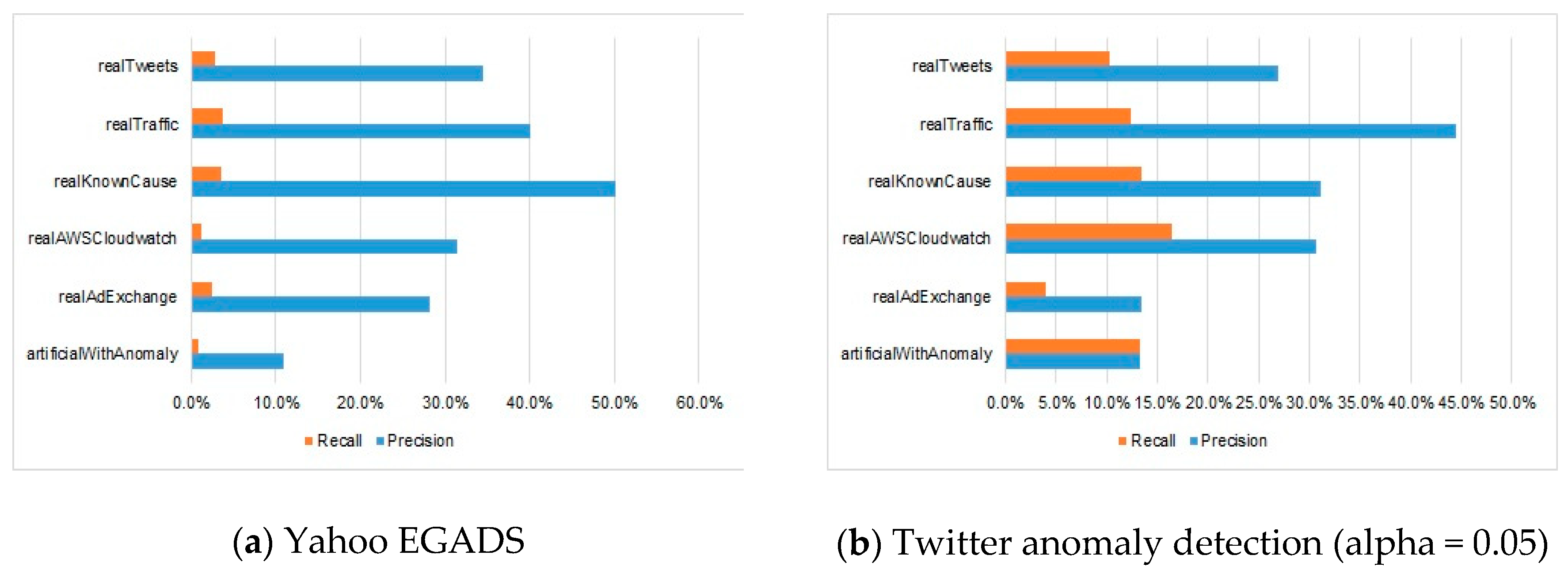
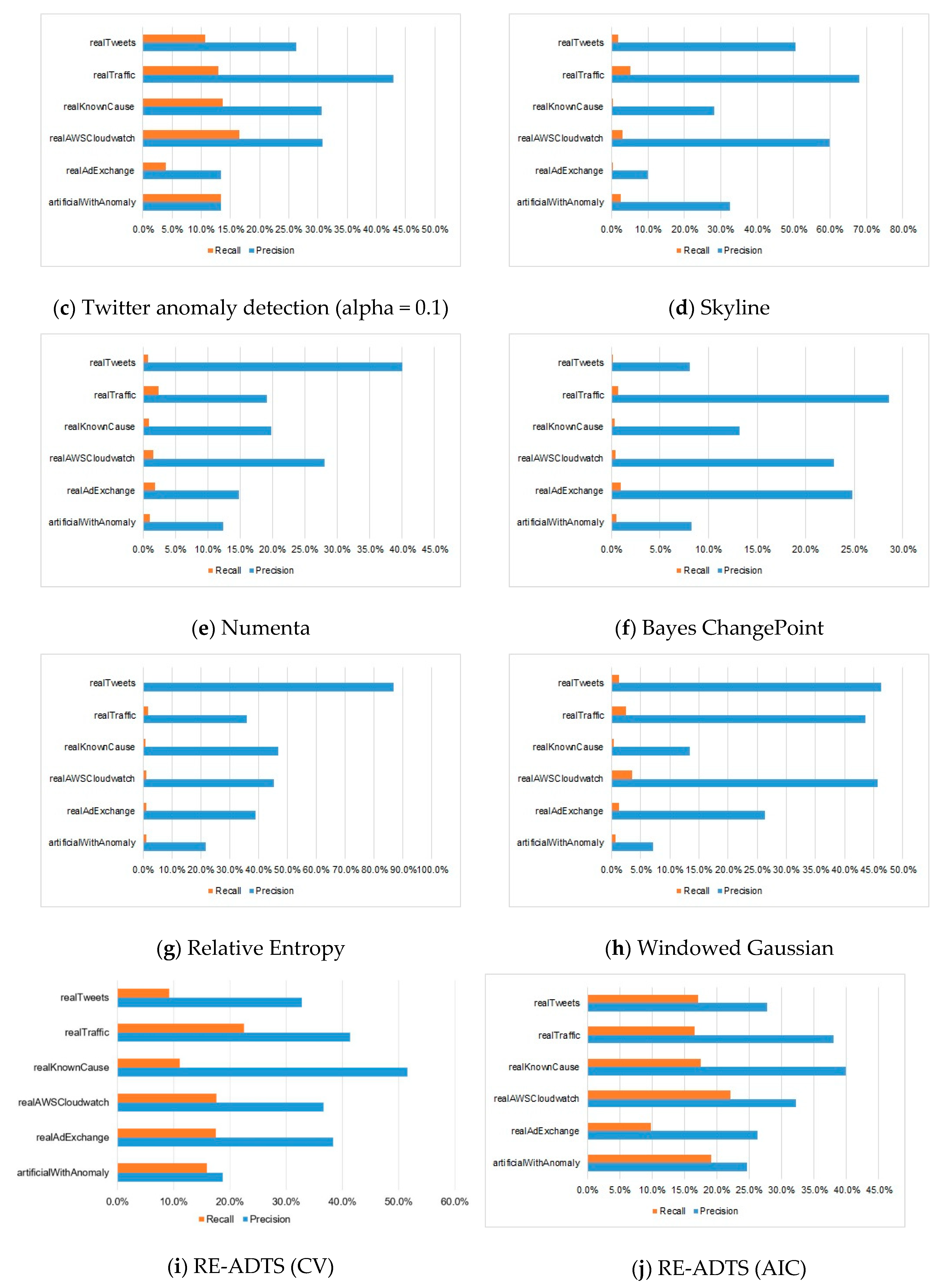
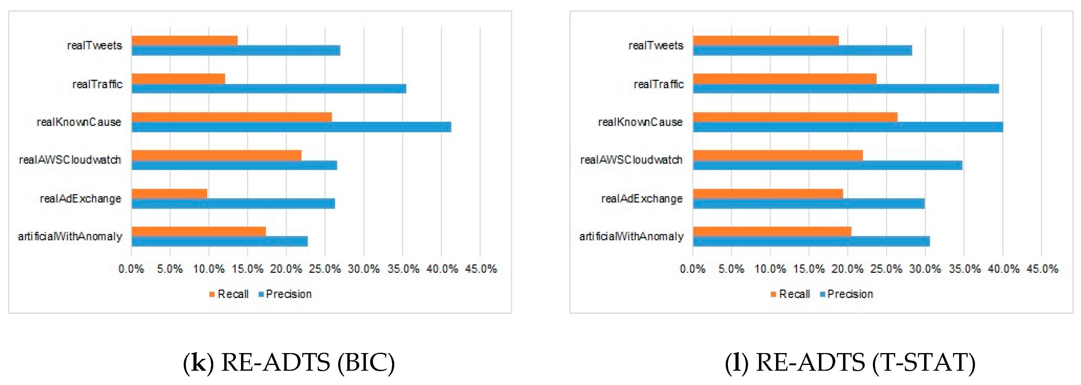
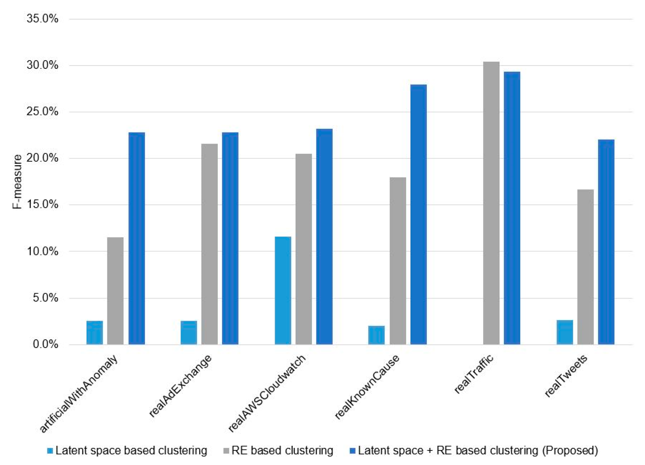
5. Experimental Results
6. Analysis and Discussion
7. Conclusions
Author Contributions
Funding
Conflicts of Interest
Appendix A

| Time-Series | Window = 5 | Window = 35 | Optimal Window (CV) | Optimal Window (AIC) | Optimal Window (BIC) | Optimal Window (T-STAT) |
|---|---|---|---|---|---|---|
| artificialWithAnomaly | 0.167091 | 0.209617 | 0.162341 | 0.207444 | 0.16837 | 0.227983 |
| realAdExchange | 0.126176 | 0.2148 | 0.211831 | 0.141578 | 0.141578 | 0.228147 |
| realAWSCloudwatch | 0.178616 | 0.243467 | 0.187829 | 0.219898 | 0.203431 | 0.231805 |
| realKnownCause | 0.203928 | 0.207285 | 0.165002 | 0.236576 | 0.284842 | 0.279474 |
| realTraffic | 0.199751 | 0.338372 | 0.281897 | 0.225306 | 0.178785 | 0.293361 |
| realTweets | 0.140052 | 0.182146 | 0.142444 | 0.195971 | 0.179773 | 0.220609 |
Appendix B

Appendix C


References
- Chandola, V.; Banerjee, A.; Kumar, V. Anomaly detection: A survey. ACM Comput. Surv. 2009, 41, 1–58. [Google Scholar] [CrossRef]
- Tan, P.N.; Steinbach, M.; Kumar, V. Anomaly Detection. In Introduction to Data Mining; Goldstein, M., Harutunian, K., Smith, K., Eds.; Pearson Education, Inc.: Boston, MA, USA, 2006; pp. 651–680. [Google Scholar]
- Goldstein, M.; Uchida, S. A comparative evaluation of unsupervised anomaly detection algorithms for multivariate data. PLoS ONE 2016, 11, e0152173. [Google Scholar] [CrossRef] [Green Version]
- Ramaswamy, S.; Rastogi, R.; Shim, K. Efficient algorithms for mining outliers from large data sets. In Proceedings of the 2000 ACM SIGMOD International Conference on Management of Data, Dallas, TX, USA, 16–18 May 2000. [Google Scholar]
- Breunig, M.M.; Kriegel, H.P.; Ng, R.T.; Sander, J. LOF: Identifying density-based local outliers. In Proceedings of the 2000 ACM SIGMOD International Conference on Management of Data, Dallas, TX, USA, 16–18 May 2000. [Google Scholar]
- He, Z.; Xu, X.; Deng, S. Discovering cluster-based local outliers. Pattern Recognit. Lett. 2003, 24, 1641–1650. [Google Scholar] [CrossRef]
- Gao, Y.; Yang, T.; Xu, M.; Xing, N. An unsupervised anomaly detection approach for spacecraft based on normal behavior clustering. In Proceedings of the Fifth International Conference on Intelligent Computation Technology and Automation, Zhangjiajie, China, 12–14 January 2012. [Google Scholar]
- Jiang, S.; Song, X.; Wang, H.; Han, J.J.; Li, Q.H. A clustering-based method for unsupervised intrusion detections. Pattern Recognit. Lett. 2006, 27, 802–810. [Google Scholar] [CrossRef]
- Li, M.; Yu, X.; Ryu, K.H.; Lee, S.; Theera-Umpon, N. Face recognition technology development with Gabor, PCA and SVM methodology under illumination normalization condition. Clust. Comput. 2018, 21, 1117–1126. [Google Scholar] [CrossRef]
- Rousseeuw, P.J.; Hubert, M. Anomaly detection by robust statistics. Data Min. Knowl. Discov. 2018, 8, e1236. [Google Scholar] [CrossRef] [Green Version]
- Hoffmann, H. Kernel PCA for novelty detection. Pattern Recognit. 2018, 40, 863–874. [Google Scholar] [CrossRef]
- Kwitt, R.; Hofmann, U. Robust methods for unsupervised PCA-based anomaly detection. In Proceedings of the IEEE/IST Workshop on Monitoring, Attack Detection and Mitigation, Tuebingen, Germany, 28–29 September 2006. [Google Scholar]
- Schölkopf, B.; Williamson, R.; Smola, A.; Shawe-Taylor, J.; Platt, J. Support Vector Method for Novelty Detection. Adv. Neural Inf. Process. Syst. 2000, 12, 582–588. [Google Scholar]
- Amer, M.; Goldstein, M.; Abdennadher, S. Enhancing One-class Support Vector Machines for Unsupervised Anomaly Detection. In Proceedings of the ACM SIGKDD Workshop on Outlier Detection and Description, Chicago, IL, USA, 1 August 2013. [Google Scholar]
- Ma, J.; Perkins, S. Time-series novelty detection using one-class support vector machines. In Proceedings of the International Joint Conference on Neural Networks, Portland, OR, USA, 20–24 July 2003. [Google Scholar] [CrossRef]
- Packard, N.H.; Crutchfield, J.P.; Farmer, J.D.; Shaw, R.S. Geometry from a time series. Phys. Rev. Lett. 1980, 45, 712. [Google Scholar] [CrossRef]
- Hu, M.; Ji, Z.; Yan, K.; Guo, Y.; Feng, X.; Gong, J.; Dong, L. Detecting anomalies in time series data via a meta-feature based approach. IEEE Access 2018, 6, 27760–27776. [Google Scholar] [CrossRef]
- Basu, S.; Meckesheimer, M. Automatic outlier detection for time series: An application to sensor data. Knowl. Inf. Syst. 2007, 11, 137–154. [Google Scholar] [CrossRef]
- Kieu, T.; Yang, B.; Jensen, C.S. Outlier detection for multidimensional time series using deep neural networks. In Proceedings of the 19th IEEE International Conference on Mobile Data Management (MDM), Aalborg, Denmark, 26–28 June 2018. [Google Scholar]
- Munir, M.; Siddiqui, S.A.; Dengel, A.; Ahmed, S. Deepant: A deep learning approach for unsupervised anomaly detection in time series. IEEE Access 2018, 7, 1991–2005. [Google Scholar] [CrossRef]
- Skyline. Available online: https://github.com/etsy/skyline (accessed on 26 November 2019).
- Laptev, N.; Amizadeh, S.; Flint, I. Generic and scalable framework for automated time-series anomaly detection. In Proceedings of the 21th ACM SIGKDD International Conference on Knowledge Discovery and Data Mining, Sydney, Australia, 10–13 August 2015. [Google Scholar]
- AnomalyDetection R package. Available online: https://github.com/twitter/AnomalyDetection (accessed on 26 November 2019).
- Rosner, B. Percentage points for a generalized ESD many-outlier procedure. Technometrics 1983, 25, 165–172. [Google Scholar] [CrossRef]
- Ahmad, S.; Lavin, A.; Purdy, S.; Agha, Z. Unsupervised real-time anomaly detection for streaming data. Neurocomputing 2017, 262, 134–147. [Google Scholar] [CrossRef]
- Amarbayasgalan, T.; Lee, J.Y.; Kim, K.R.; Ryu, K.H. Deep Autoencoder Based Neural Networks for Coronary Heart Disease Risk Prediction. In Heterogeneous Data Management, Polystores, and Analytics for Healthcare; Springer: Los Angeles, CA, USA, 2019; Volume 11721, pp. 237–248. [Google Scholar]
- Batbaatar, E.; Li, M.; Ryu, K.H. Semantic-Emotion Neural Network for Emotion Recognition from Text. IEEE Access 2019, 7, 111866–111878. [Google Scholar] [CrossRef]
- Munkhdalai, L.; Munkhdalai, T.; Park, K.H.; Amarbayasgalan, T.; Erdenebaatar, E.; Park, H.W.; Ryu, K.H. An End-to-End Adaptive Input Selection with Dynamic Weights for Forecasting Multivariate Time Series. IEEE Access 2019, 7, 99099–99114. [Google Scholar] [CrossRef]
- Amarbayasgalan, T.; Jargalsaikhan, B.; Ryu, K.H. Unsupervised novelty detection using deep autoencoders with density based clustering. Appl. Sci. 2018, 8, 1468. [Google Scholar] [CrossRef] [Green Version]
- Kraslawski, A.; Turunen, I. European Symposium on Computer Aided Process Engineering-13: 36th European Symposium of the Working Party on Computer Aided Process Engineering; Elsevier: Oxford, UK, 2003; pp. 462–463. [Google Scholar]
- Autoregressive Model. Available online: https://en.wikipedia.org/wiki/Autoregressive_model (accessed on 26 November 2019).
- Akaike, H. A new look at the statistical model identification. IEEE Trans. Autom. Control 1974, 19, 716–723. [Google Scholar] [CrossRef]
- Statsmodels. Available online: https://www.statsmodels.org/stable/generated/statsmodels.tsa.ar_model.AR.fit.html (accessed on 7 July 2020).
- Ding, J.; Tarokh, V.; Yang, Y. Model selection techniques: An overview. IEEE Signal Process. Mag. 2018, 35, 16–34. [Google Scholar] [CrossRef] [Green Version]
- Kim, H.; Hirose, A. Unsupervised Fine Land Classification Using Quaternion Autoencoder-Based Polarization Feature Extraction and Self-Organizing Mapping. IEEE Trans. Geosci. Remote Sens. 2017, 56, 1839–1851. [Google Scholar] [CrossRef]
- Ester, M.; Kriegel, H.P.; Sander, J.; Xu, X. A Density-Based Algorithm for Discovering Clusters in Large Spatial Databases with Noise. In Proceedings of the Second International Conference on Knowledge Discovery and Data Mining, Portland, OR, USA, 2–4 August 1996. [Google Scholar]
- Jin, C.H.; Na, H.J.; Piao, M.; Pok, G.; Ryu, K.H. A Novel DBSCAN-based Defect Pattern Detection and Classification Framework for Wafer Bin Map. IEEE Trans. Semicond. Manuf. 2019, 32, 286–292. [Google Scholar] [CrossRef]
- Otsu, N. A Threshold Selection Method from Gray-Level Histograms. IEEE Trans. Syst. Man Cybern. 1979, 9, 62–66. [Google Scholar] [CrossRef] [Green Version]
- Hanley, J.A.; McNeil, B.J. The meaning and use of the area under a receiver operating characteristic (ROC) curve. Radiology 1982, 143, 29–36. [Google Scholar] [CrossRef] [PubMed] [Green Version]
- Home of the HTM Community. Available online: https://www.numenta.org/ (accessed on 26 November 2019).
- Kingma, D.P.; Ba, J. Adam: A method for stochastic optimization. In Proceedings of the 3rd International Conference for Learning Representations, San Diego, CA, USA, 7–9 May 2014. [Google Scholar]
- Adams, R.P.; MacKay, D.J. Bayesian online changepoint detection. arXiv 2017, arXiv:0710.3742. [Google Scholar]
- Wang, C.; Viswanathan, K.; Choudur, L.; Talwar, V.; Satterfield, W.; Schwan, K. Statistical techniques for Online Anomaly Detection in Data Centers. In Proceedings of the 12th IFIP/IEEE International Symposium on Integrated Network Management (IM 2011) and Workshops, Dublin, Ireland, 23–27 May 2011. [Google Scholar]


| Time-Series | CV | AIC | BIC | T-STAT |
|---|---|---|---|---|
| Artificial With Anomaly | 21 | 21 | 11 | 27 |
| realAdExchange | 23 | 18 | 14 | 20 |
| realAWSCloudwatch | 19 | 22 | 14 | 25 |
| realKnownCause | 21 | 24 | 28 | 33 |
| realTraffic | 19 | 9 | 4 | 21 |
| realTweets | 18 | 29 | 17 | 34 |
| Time-Series | Yahoo EGADS | Twitter Anomaly Detection (alpha = 0.05) | Twitter Anomaly Detection (alpha = 0.1) | Skyline | Numenta | Bayes ChangePoint | Relative Entropy | Windowed Gaussian | RE-ADTS (CV) | RE-ADTS (AIC) | RE-ADTS (BIC) | RE-ADTS (T-STAT) | |||||||||||||
|---|---|---|---|---|---|---|---|---|---|---|---|---|---|---|---|---|---|---|---|---|---|---|---|---|---|
| P. | R. | P. | R. | P. | R. | P. | R. | P. | R. | P. | R. | P. | R. | P. | R. | P. | R. | P. | R. | P. | R. | P. | R. | ||
| artificialWithAnomaly | art_daily_flatmiddle | 0.0 | 0.0 | 9.4 | 9.4 | 9.4 | 9.4 | 0.0 | 0.0 | 13.3 | 0.50 | 7.4 | 0.50 | 37.5 | 2.23 | 0.0 | 0.00 | 10.0 | 0.74 | 7.84 | 4.0 | 0.0 | 0.0 | 8.8 | 0.7 |
| art_daily_jumpsdown | 0.0 | 0.0 | 2.0 | 2.0 | 2.0 | 2.0 | 0.0 | 0.0 | 0.0 | 0.00 | 8.0 | 0.50 | 16.7 | 0.74 | 0.0 | 0.00 | 7.79 | 4.71 | 3.7 | 2.0 | 3.7 | 1.7 | 8.3 | 3.7 | |
| art_daily_jumpsup | 0.0 | 0.0 | 28.8 | 28.8 | 28.8 | 28.8 | 95.2 | 14.6 | 30.0 | 1.49 | 8.0 | 0.50 | 47.8 | 2.73 | 0.0 | 0.00 | 38.4 | 33.0 | 49.2 | 31.0 | 86.0 | 27.5 | 71.0 | 32.8 | |
| art_daily_nojump | 0.0 | 0.0 | 1.7 | 1.7 | 1.7 | 1.7 | 0.0 | 0.0 | 0.0 | 0.00 | 3.8 | 0.25 | 0.0 | 0.00 | 0.0 | 0.00 | 7.78 | 3.47 | 0.0 | 0.0 | 0.0 | 0.0 | 8.0 | 5.0 | |
| art_increase_spike_density | 0.0 | 0.0 | 11.7 | 11.7 | 11.7 | 11.7 | 100 | 0.2 | 6.1 | 0.50 | 10.0 | 0.99 | 0.0 | 0.00 | 0.0 | 0.00 | 12.5 | 7.94 | 11.8 | 23.8 | 11.3 | 26.1 | 11.3 | 26.1 | |
| art_load_balancer_spikes | 65.5 | 4.7 | 26.3 | 26.3 | 26.3 | 26.3 | 0.0 | 0.0 | 25.0 | 3.97 | 12.5 | 0.25 | 27.3 | 0.74 | 42.9 | 4.47 | 35.6 | 45.6 | 75.3 | 53.8 | 35.6 | 48.9 | 76.1 | 54.6 | |
| Average | 10.9 | 0.8 | 13.3 | 13.3 | 13.3 | 13.3 | 32.5 | 2.5 | 12.4 | 1.08 | 8.3 | 0.50 | 21.5 | 1.08 | 7.1 | 0.74 | 18.7 | 15.9 | 24.6 | 19.1 | 22.8 | 17.4 | 30.6 | 20.5 | |
| realAdExchange | exchange-2_cpc | 7.7 | 0.6 | 0.0 | 0.0 | 0.0 | 0.0 | 0.0 | 0.0 | 0.0 | 0.0 | 0.0 | 0.0 | 15.4 | 1.23 | 0.0 | 0.0 | 0.0 | 0.0 | 0.0 | 0.0 | 0.0 | 0.0 | 0.0 | 0.0 |
| exchange-2_cpm | 37.5 | 1.9 | 9.8 | 6.8 | 9.8 | 6.8 | 0.0 | 0.0 | 13.3 | 2.5 | 40.0 | 1.2 | 0.0 | 0.0 | 0.0 | 0.0 | 50.0 | 0.62 | 20.4 | 6.17 | 20.4 | 6.17 | 20.4 | 6.17 | |
| exchange-3_cpc | 36.4 | 5.2 | 21.3 | 8.5 | 21.3 | 8.5 | 0.0 | 0.0 | 12.5 | 2 | 50.0 | 1.3 | 42.9 | 1.96 | 55.6 | 3.27 | 59.5 | 49.0 | 39.5 | 11.1 | 39.5 | 11.1 | 60.2 | 48.4 | |
| exchange-3_cpm | 11.1 | 0.7 | 2.3 | 0.7 | 2.3 | 0.7 | 0.0 | 0.0 | 8.3 | 1.3 | 20.0 | 0.7 | 33.3 | 1.31 | 25.0 | 0.65 | 32.0 | 16.3 | 28.2 | 15.7 | 28.2 | 15.7 | 27.9 | 15.7 | |
| exchange-4_cpc | 30.8 | 2.4 | 28.6 | 4.8 | 28.6 | 4.8 | 0.0 | 0.0 | 21.4 | 1.8 | 16.7 | 1.2 | 75.0 | 1.82 | 33.3 | 1.82 | 51.4 | 32.7 | 33.3 | 12.1 | 33.3 | 12.1 | 34.9 | 32.1 | |
| exchange-4_cpm | 46.2 | 3.7 | 18.5 | 3 | 18.5 | 3.0 | 60.0 | 1.8 | 33.3 | 3.7 | 22.2 | 1.2 | 66.7 | 1.22 | 44.4 | 2.44 | 37.0 | 6.10 | 35.9 | 14.0 | 35.9 | 14.0 | 36.5 | 14.0 | |
| Average | 28.3 | 2.4 | 13.4 | 3.8 | 13.4 | 4.1 | 10.0 | 0.3 | 14.8 | 1.9 | 24.8 | 0.9 | 38.9 | 1.3 | 26.4 | 1.4 | 38.3 | 17.4 | 26.2 | 9.9 | 26.2 | 9.9 | 30.0 | 19.4 | |
| realAWSCloudwatch | ec2_cpu_utilization_5f5533 | 50.0 | 0.5 | 100 | 0.2 | 100 | 0.2 | 100 | 0.2 | 43.8 | 1.7 | 50.0 | 0.2 | 77.8 | 1.74 | 0.0 | 0.0 | 96.6 | 14.1 | 86.2 | 20.1 | 86.2 | 20.1 | 86.5 | 20.6 |
| ec2_cpu_utilization_24ae8d | 31.8 | 1.7 | 10.4 | 10.4 | 10.4 | 10.4 | 40.0 | 0.5 | 23.5 | 1 | 23.5 | 1.0 | 33.3 | 0.25 | 11.8 | 0.5 | 18.7 | 9.70 | 28.9 | 3.23 | 28.9 | 3.23 | 28.9 | 3.23 | |
| ec2_cpu_utilization_53ea38 | 37.1 | 3.2 | 38.9 | 3.5 | 44.4 | 5.0 | 0.0 | 0.0 | 14.3 | 1 | 18.8 | 0.7 | 50 | 0.75 | 28.6 | 0.5 | 84.3 | 6.72 | 19.2 | 27.1 | 19.2 | 27.1 | 19.2 | 27.1 | |
| ec2_cpu_utilization_77c1ca | 0.0 | 0.0 | 17.4 | 17.4 | 17.4 | 17.4 | 60 | 1.5 | 11.5 | 1.5 | 0.0 | 0.0 | 11.1 | 0.5 | 0.0 | 0.0 | 0.0 | 0.0 | 14.3 | 37.5 | 16.4 | 31.5 | 18.8 | 14.6 | |
| ec2_cpu_utilization_825cc2 | 0.0 | 0.0 | 79.1 | 30.9 | 79.1 | 30.9 | 100 | 8.7 | 52.2 | 3.5 | 50.0 | 0.6 | 88.9 | 2.33 | 97.3 | 10.5 | 74.0 | 33.2 | 69.9 | 37.3 | 73.9 | 33.8 | 69.3 | 38.2 | |
| ec2_cpu_utilization_ac20cd | 0.0 | 0.0 | 46.2 | 46.2 | 46.2 | 46.2 | 71.4 | 5.0 | 27.3 | 1.5 | 50.0 | 0.2 | 31.6 | 1.49 | 78.1 | 6.2 | 32.7 | 48.6 | 30.4 | 43.7 | 31.4 | 45.7 | 30.4 | 43.7 | |
| ec2_cpu_utilization_fe7f93_ | 27.0 | 2.5 | 15.4 | 15.3 | 15.4 | 15.3 | 42.1 | 5.9 | 13.5 | 1.2 | 20.0 | 0.5 | 33.3 | 0.74 | 54.5 | 1.48 | 15.3 | 13.0 | 23.4 | 15.8 | 9.52 | 17.8 | 31.5 | 18.5 | |
| ec2_disk_write_bytes_1ef3de | 13.9 | 1.1 | 13.3 | 13.3 | 13.3 | 13.3 | 20.9 | 1.9 | 15.4 | 1.3 | 11.8 | 0.4 | 27.3 | 0.63 | 12.9 | 1.9 | 17.1 | 10.7 | 14.2 | 6.98 | 15.1 | 13.5 | 14.4 | 16.7 | |
| ec2_disk_write_bytes_c0d644 | 24.0 | 1.5 | 18.4 | 18.3 | 18.4 | 18.3 | 75.0 | 1.5 | 29.8 | 3.5 | 0.0 | 0.0 | 50.0 | 1.73 | 38.2 | 3.21 | 35.2 | 4.44 | 38.5 | 13.6 | 24.1 | 16 | 37.8 | 11.9 | |
| ec2_network_in_5abac7 | 41.0 | 3.0 | 21.6 | 21.5 | 21.6 | 21.5 | 29.2 | 1.5 | 30.6 | 2.3 | 5.3 | 0.2 | 0.0 | 0.0 | 80.0 | 0.99 | 38.3 | 24.0 | 37.8 | 29.1 | 0.0 | 0.0 | 38.4 | 29.7 | |
| ec2_network_in_257a54 | 100 | 1.5 | 18.9 | 18.9 | 18.9 | 18.9 | 100 | 1.2 | 60.0 | 1.5 | 0.0 | 0.0 | 75.0 | 0.74 | 23.8 | 4.01 | 0.0 | 0.0 | 0.0 | 0.0 | 21.2 | 32.7 | 0.0 | 0.0 | |
| elb_request_count_8c0756 | 39.0 | 2.0 | 32.1 | 2.2 | 26.3 | 2.5 | 80.0 | 1.0 | 17.4 | 1 | 16.7 | 0.7 | 20.0 | 0.3 | 50.0 | 0.25 | 62.2 | 15.1 | 40.2 | 17.9 | 27.1 | 9.0 | 50.0 | 17.4 | |
| grok_asg_anomaly | 17.0 | 0 | 8.4 | 8.4 | 8.4 | 8.4 | 40.0 | 3.4 | 34.6 | 1.9 | 27.3 | 0.6 | 62.5 | 1.1 | 92.0 | 14.8 | 7.42 | 13.5 | 5.7 | 10.1 | 6.1 | 10.8 | 5.6 | 10.0 | |
| iio_us-east-1_i-a2eb1cd9 | 0.0 | 0.0 | 32.3 | 15.9 | 32.3 | 16.7 | 0.0 | 0.0 | 0.0 | 0.0 | 0.0 | 0.0 | 0.0 | 0.0 | 0.0 | 0.0 | 0.0 | 0.0 | 18.5 | 4.0 | 35.1 | 15.9 | 37.1 | 10.3 | |
| rds_cpu_utilization_cc0c53 | 100 | 0.0 | 32.8 | 32.8 | 32.8 | 32.8 | 100 | 10.9 | 37.5 | 1.5 | 20.0 | 0.2 | 77.8 | 1.8 | 98.0 | 12.4 | 31.5 | 74.8 | 31.7 | 74.9 | 31.8 | 74.9 | 31.7 | 74.9 | |
| rds_cpu_utilization_e47b3b | 22.0 | 0.0 | 7.2 | 7.2 | 7.2 | 7.2 | 100 | 5.7 | 36.4 | 1 | 50.0 | 0.5 | 87.5 | 1.8 | 66.7 | 0.5 | 71.6 | 13.1 | 56.4 | 13.2 | 0.0 | 0.0 | 57.1 | 14.9 | |
| Average | 31.4 | 1.2 | 30.8 | 16.4 | 30.7 | 16.6 | 59.9 | 3.1 | 28.0 | 1.6 | 22.9 | 0.4 | 45.4 | 0.1 | 45.7 | 3.6 | 36.6 | 17.6 | 32.2 | 22.2 | 26.6 | 22.0 | 34.8 | 22.0 | |
| realKnownCause | ambient_temperature_system_failure | 89.0 | 9.0 | 0.0 | 0.0 | 0.0 | 0.0 | 0.0 | 0.0 | 20.5 | 1.1 | 0.0 | 0.0 | 11.1 | 0.41 | 0.0 | 0.0 | 48.1 | 14.3 | 40.4 | 20.4 | 43.0 | 19.1 | 40.4 | 20.4 |
| cpu_utilization_asg_misconfiguration | 0.0 | 0.0 | 23.4 | 28.2 | 23.4 | 28.2 | 0.0 | 0.0 | 38.9 | 0.9 | 7.3 | 0.5 | 66.7 | 0.8 | 0.0 | 0.0 | 43.1 | 2.74 | 35.4 | 25.4 | 47.8 | 76.1 | 39.2 | 79.5 | |
| ec2_request_latency_system_failure | 38.0 | 5.0 | 93.3 | 4.0 | 93.3 | 4.0 | 100 | 1.4 | 47.6 | 2.9 | 28.6 | 0.6 | 100 | 1.45 | 88.9 | 2.4 | 97.0 | 9.54 | 35.6 | 19.9 | 47.8 | 9.6 | 45.6 | 19.7 | |
| machine_ temperature_system_failure | 100 | 5.0 | 80.0 | 40.4 | 76.2 | 42.0 | 97.0 | 1.4 | 0.0 | 0.0 | 20.0 | 0.0 | 64.3 | 0.79 | 0.0 | 0.0 | 83.4 | 39.2 | 82.5 | 26.4 | 66.6 | 46.4 | 74.8 | 36.6 | |
| nyc_taxi_labeled_5 | 89.0 | 2.0 | 0.0 | 0.0 | 0.0 | 0.0 | 0.0 | 0.0 | 21.2 | 0.7 | 0.0 | 0.0 | 76.9 | 0.97 | 0.0 | 0.0 | 68.5 | 3.57 | 62.3 | 15.7 | 65.2 | 19.2 | 67.3 | 17.3 | |
| rogue_agent_key_hold | 17.0 | 1.0 | 13.3 | 13.2 | 13.3 | 13.2 | 0.0 | 0.0 | 5.26 | 0.5 | 25.0 | 1.1 | 8.33 | 0.53 | 0.0 | 0.0 | 3.43 | 3.68 | 13.8 | 9.0 | 8.6 | 4.8 | 5.8 | 7.4 | |
| rogue_agent_key_updown | 18.0 | 1.0 | 8.5 | 8.5 | 8.5 | 8.5 | 0.0 | 0.0 | 5.56 | 0.2 | 11.8 | 0.4 | 0.0 | 0.0 | 5.3 | 0.2 | 16.9 | 4.53 | 9.5 | 6.3 | 9.7 | 6.5 | 7.1 | 4.6 | |
| Average | 50.1 | 3.5 | 31.2 | 13.5 | 30.7 | 13.7 | 28.1 | 0.4 | 19.9 | 0.9 | 13.2 | 0.4 | 46.8 | 0.7 | 13.5 | 0.4 | 51.5 | 11.1 | 39.9 | 17.6 | 41.3 | 25.9 | 40.0 | 26.5 | |
| realTraffic | occupancy_6005 | 12.5 | 0.0 | 14.3 | 1.3 | 15.4 | 1.7 | 50.0 | 0.4 | 6.25 | 0.4 | 0.0 | 0.0 | 4.6 | 0.42 | 0.0 | 0.0 | 25.5 | 10.4 | 14.4 | 13 | 14.6 | 7.5 | 13.6 | 15.5 |
| occupancy_t4013 | 58.3 | 6.0 | 78.6 | 4.4 | 73.3 | 4.4 | 100 | 4.0 | 26.3 | 2.0 | 0.0 | 0.0 | 57.1 | 3.2 | 75.0 | 1.2 | 64.9 | 25.2 | 34.5 | 11.6 | 35.5 | 10.8 | 38.7 | 26.8 | |
| speed_6005 | 17.6 | 3.0 | 60.0 | 1.3 | 60.0 | 1.3 | 100 | 1.3 | 17.4 | 1.7 | 33.3 | 0.4 | 28.6 | 0.8 | 50.0 | 0.4 | 16.2 | 5.86 | 27.8 | 8.4 | 26.7 | 8.4 | 30.1 | 14.2 | |
| speed_7578 | 88.9 | 7.0 | 62.0 | 26.7 | 58.6 | 29.3 | 82.6 | 16.4 | 26.9 | 6.0 | 75.0 | 2.6 | 44.4 | 3.5 | 84.6 | 9.5 | 61.8 | 51.7 | 80.0 | 44.8 | 83.9 | 22.4 | 79.7 | 44.0 | |
| speed_t4013 | 53.3 | 6.0 | 55.1 | 10.8 | 50.8 | 12.0 | 94.4 | 6.8 | 34.5 | 4.0 | 75.0 | 1.2 | 54.5 | 2.4 | 87.5 | 5.6 | 56.5 | 41.6 | 57.1 | 16.0 | 36.6 | 18.0 | 58.3 | 38.0 | |
| TravelTime_387 | 28.0 | 3.0 | 24.8 | 24.9 | 24.8 | 24.9 | 50.0 | 7.2 | 14.8 | 1.6 | 0.0 | 0.0 | 50.0 | 1.2 | 8.3 | 0.4 | 30.3 | 9.64 | 32.4 | 14.1 | 30.4 | 9.6 | 32.4 | 14.1 | |
| TravelTime_451 | 22.2 | 1.8 | 17.1 | 17.1 | 17.1 | 17.1 | 0.0 | 0.0 | 7.4 | 0.9 | 16.7 | 0.5 | 12.5 | 0.5 | 0.0 | 0.0 | 33.7 | 12.9 | 20.2 | 8.3 | 20.2 | 8.3 | 24.2 | 13.8 | |
| Average | 40.1 | 3.8 | 44.6 | 12.3 | 42.9 | 12.9 | 68.2 | 5.2 | 19.1 | 2.4 | 28.6 | 0.7 | 36.0 | 1.7 | 43.6 | 2.4 | 41.3 | 22.4 | 38.1 | 16.6 | 35.4 | 12.1 | 39.6 | 23.8 | |
| realTweets | Twitter_volume_AAPL | 49.3 | 4.2 | 39.4 | 24.2 | 38.8 | 25.0 | 66.4 | 4.7 | 47.1 | 1 | 12.8 | 0.3 | 100 | 0.31 | 58.3 | 2.6 | 40.5 | 9.95 | 31.6 | 13.9 | 35.7 | 10.7 | 38.7 | 14.5 |
| Twitter_volume_AMZN | 38.7 | 2.9 | 38.8 | 2.5 | 37.6 | 2.8 | 32.6 | 0.9 | 30.8 | 0.5 | 18.2 | 0.3 | 100 | 0.25 | 31.3 | 0.6 | 38.5 | 10.1 | 32.3 | 18.5 | 35.1 | 16.4 | 31.5 | 23.0 | |
| Twitter_volume_CRM | 68.7 | 3.6 | 53.9 | 8.6 | 52.2 | 9.7 | 73.5 | 1.6 | 50 | 0.5 | 6.38 | 0.2 | 100 | 0.19 | 83.3 | 0.6 | 55.0 | 18.5 | 38.6 | 24.4 | 41.4 | 22.9 | 40.2 | 24.3 | |
| Twitter_volume_CVS | 37.5 | 2.4 | 11.6 | 12.1 | 11.6 | 12.1 | 55.6 | 0.7 | 48 | 0.8 | 0.0 | 0.0 | 100 | 0.26 | 51.2 | 1.4 | 38.2 | 13.3 | 36.2 | 12.6 | 21.5 | 12.8 | 37.1 | 17.9 | |
| Twitter_volume_FB | 9.6 | 0.8 | 10.8 | 3.0 | 10.6 | 3.3 | 17.9 | 0.4 | 26.3 | 0.3 | 15 | 0.4 | 75.0 | 0.19 | 22.2 | 0.4 | 12.3 | 2.78 | 15.3 | 11.7 | 15.3 | 8.7 | 16.1 | 12.7 | |
| Twitter_volume_GOOG | 28.7 | 5.4 | 33.7 | 9.1 | 31.6 | 10.1 | 59.7 | 2.8 | 30.3 | 0.7 | 10.8 | 0.3 | 80.0 | 0.28 | 65.7 | 1.6 | 49.4 | 13.4 | 35.5 | 24.0 | 34.2 | 18.4 | 32.5 | 23.1 | |
| Twitter_volume_IBM | 25.7 | 1.6 | 18.1 | 3.6 | 17.8 | 3.7 | 22.4 | 1.1 | 41.7 | 0.6 | 13 | 0.4 | 62.5 | 0.31 | 34.1 | 0.9 | 18.4 | 4.59 | 18.7 | 16.0 | 18.2 | 14.2 | 18.6 | 16.0 | |
| Twitter_volume_KO | 33.6 | 2.3 | 22.0 | 6.9 | 21.8 | 7.6 | 42.5 | 2.3 | 28.6 | 0.4 | 2.22 | 0.1 | 50.0 | 0.06 | 36.1 | 1.4 | 18.8 | 5.99 | 17.7 | 9.33 | 17.3 | 7.3 | 17.6 | 9.5 | |
| Twitter_volume_PFE | 30.9 | 2.9 | 17.7 | 17.7 | 17.7 | 17.7 | 100 | 0.3 | 44.4 | 0.5 | 0.0 | 0.0 | 100 | 0.19 | 33.3 | 0.4 | 32.3 | 6.99 | 28.2 | 21.0 | 26.6 | 16.6 | 28.3 | 20.7 | |
| Twitter_volume_UPS | 22.5 | 1.5 | 22.6 | 14.5 | 22.6 | 14.5 | 34.3 | 4.4 | 52.7 | 1.8 | 2.17 | 0.1 | 100 | 0.57 | 47.1 | 3.6 | 23.8 | 5.74 | 23.1 | 19.6 | 23.6 | 9.7 | 21.8 | 26.2 | |
| Average | 34.5 | 2.8 | 26.9 | 10.2 | 26.3 | 10.6 | 50.5 | 1.9 | 40.0 | 0.7 | 8.1 | 0.2 | 86.8 | 0.3 | 46.3 | 1.4 | 32.7 | 9.15 | 27.7 | 17.1 | 26.9 | 13.8 | 28.2 | 18.8 | |
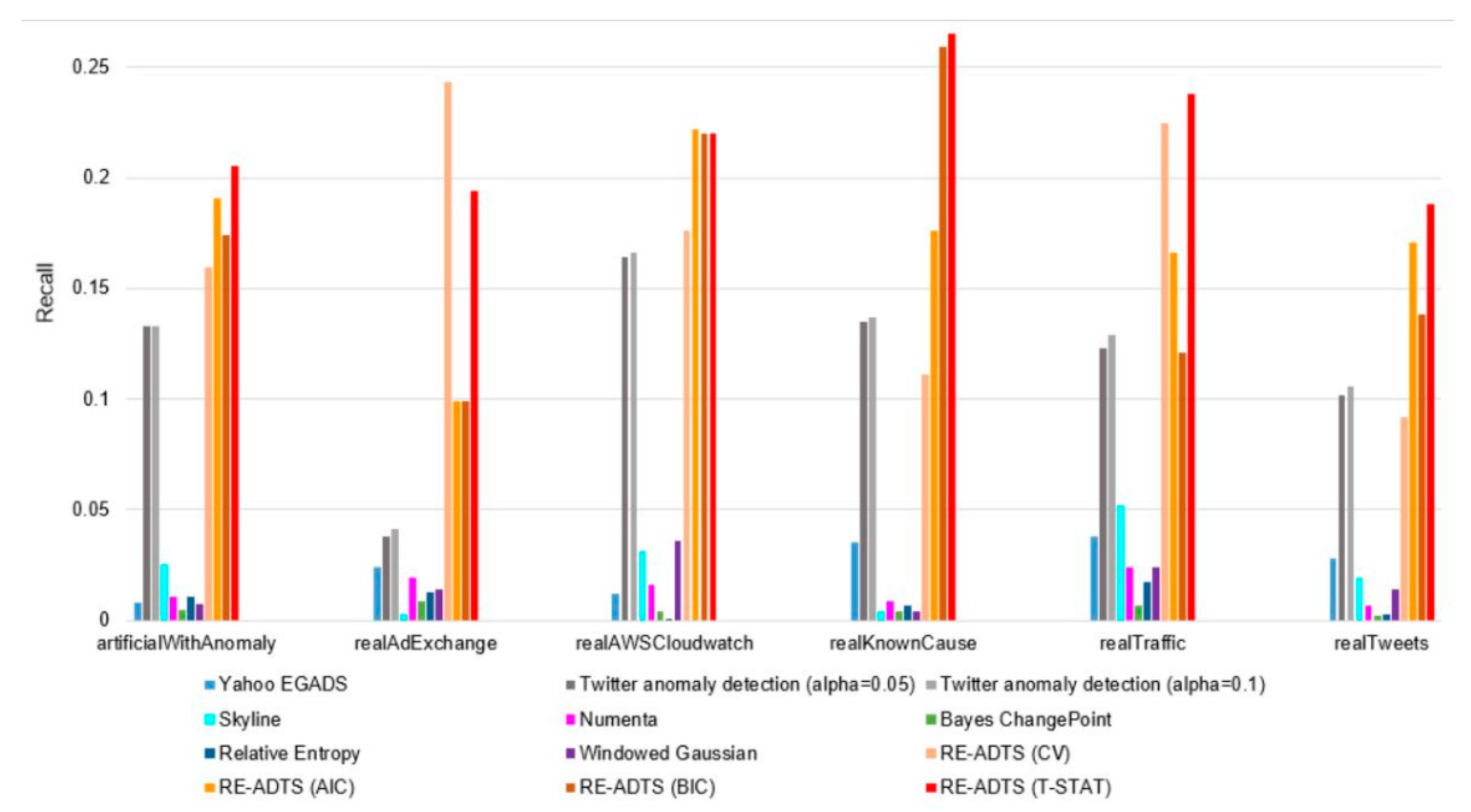
| Time-Series | Yahoo EGADS | Twitter Anomaly Detection (alpha = 0.05) | Twitter Anomaly Detection (alpha = 0.1) | Skyline | Numenta | Bayes ChangePoint | Relative Entropy | Windowed Gaussian | RE-ADTS (CV) | RE-ADTS (AIC) | RE-ADTS (BIC) | RE-ADTS (T-STAT) |
|---|---|---|---|---|---|---|---|---|---|---|---|---|
| artificialWithAnomaly | 1.5 | 13.3 | 13.3 | 4.3 | 1.9 | 0.9 | 2 | 1.3 | 16.2 | 20.7 | 16.8 | 22.8 |
| realAdExchange | 4.4 | 5.8 | 5.8 | 0.6 | 3.3 | 1.8 | 2.4 | 2.6 | 21.1 | 14.2 | 14.2 | 22.8 |
| realAWSCloudwatch | 2.2 | 17.9 | 18.1 | 5.7 | 3 | 0.8 | 1.9 | 6.4 | 18.7 | 22 | 20.3 | 23.2 |
| realKnownCause | 6.4 | 15.5 | 15.6 | 0.8 | 1.7 | 0.7 | 1.4 | 0.7 | 16.5 | 23.7 | 28.5 | 27.9 |
| realTraffic | 6.9 | 15.8 | 16.3 | 9.1 | 4.2 | 1.3 | 3.2 | 4.5 | 28.1 | 22.5 | 17.9 | 29.3 |
| realTweets | 5.1 | 13.2 | 13.7 | 3.6 | 1.4 | 0.4 | 0.5 | 2.6 | 14.2 | 20.8 | 18 | 22.1 |
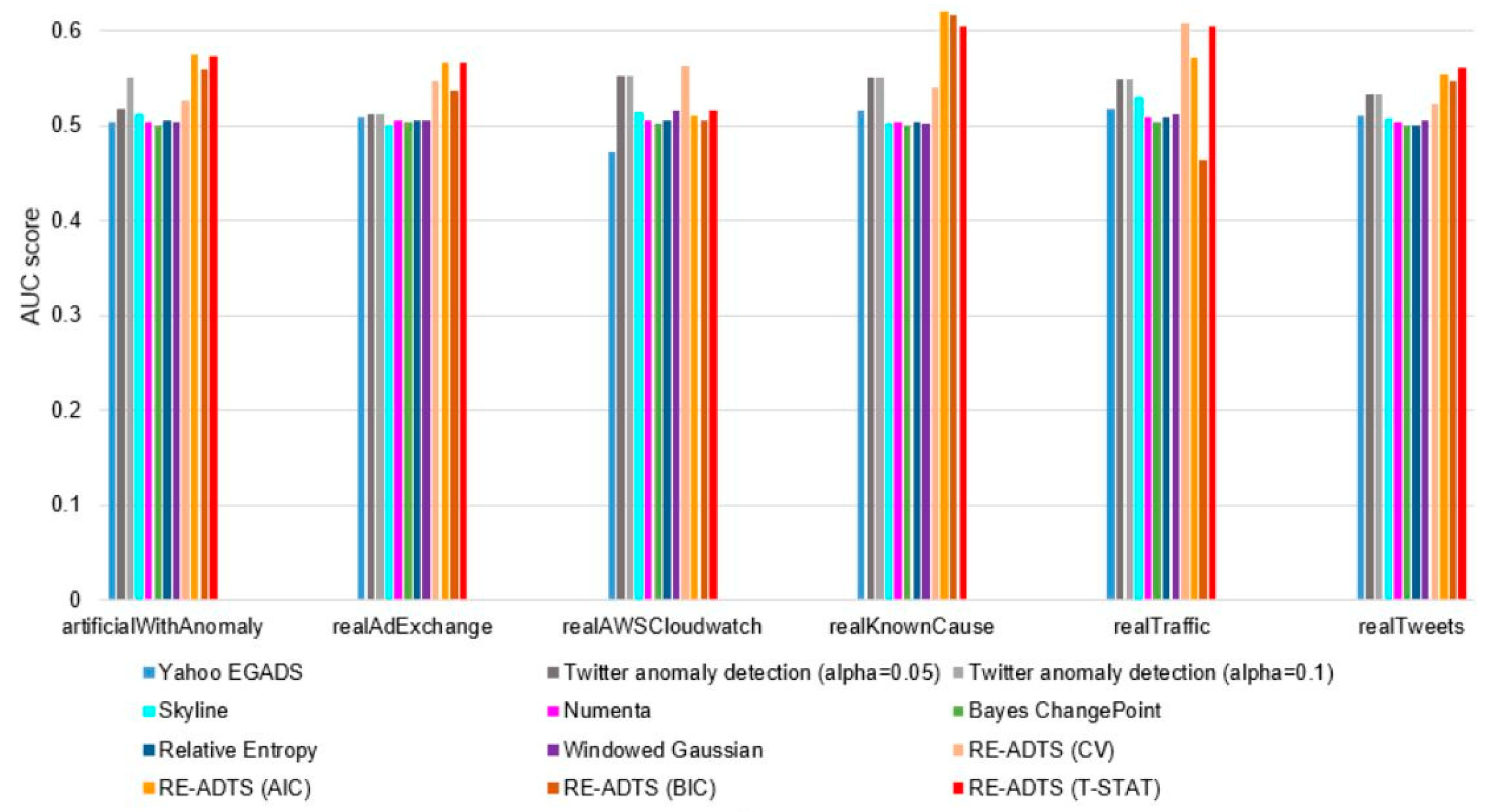
| Time-Series | Yahoo EGADS | Twitter Anomaly Detection (alpha = 0.05) | Twitter Anomaly Detection (alpha = 0.1) | Skyline | Numenta | Bayes ChangePoint | Relative Entropy | Windowed Gaussian | RE-ADTS (CV) | RE-ADTS (AIC) | RE-ADTS (BIC) | RE-ADTS (T-STAT) |
|---|---|---|---|---|---|---|---|---|---|---|---|---|
| artificialWithAnomaly | 50.4 | 51.8 | 55.0 | 51.3 | 50.4 | 50.1 | 50.5 | 50.3 | 52.6 | 57.5 | 56.0 | 57.3 |
| realAdExchange | 50.9 | 51.2 | 51.3 | 50.1 | 50.6 | 50.3 | 50.5 | 50.6 | 54.7 | 56.7 | 53.7 | 56.7 |
| realAWSCloudwatch | 47.2 | 55.3 | 55.3 | 51.4 | 50.6 | 50.2 | 50.5 | 51.6 | 56.3 | 51.0 | 50.5 | 51.6 |
| realKnownCause | 51.6 | 55.0 | 55.1 | 50.2 | 50.4 | 50.1 | 50.3 | 50.2 | 53.9 | 62.0 | 61.6 | 60.4 |
| realTraffic | 51.8 | 54.9 | 54.9 | 52.9 | 50.9 | 50.3 | 50.9 | 51.3 | 60.7 | 57.2 | 46.3 | 60.5 |
| realTweets | 51.1 | 53.3 | 53.3 | 50.8 | 50.3 | 50.1 | 50.1 | 50.6 | 52.3 | 55.5 | 54.7 | 56.1 |
| Time-Series | ContextOSE | Numenta | NumentaTM | Skyline | Twitter Anomaly Detection | DeepAnT | RE-ADTS (T-STAT) | |||||||||||||||
|---|---|---|---|---|---|---|---|---|---|---|---|---|---|---|---|---|---|---|---|---|---|---|
| P. | R. | F. | P. | R. | F. | P. | R. | F. | P. | R. | F. | P. | R. | F. | P. | R. | F. | P. | R. | F. | ||
| realAdExchange | exchange-2_cpc | 0.500 | 0.006 | 0.012 | 0.000 | 0.000 | 0.000 | 0.000 | 0.000 | 0.000 | 0.000 | 0.000 | 0.000 | 0.000 | 0.000 | 0.000 | 0.030 | 0.330 | 0.055 | 0.000 | 0.000 | 0.000 |
| exchange-3_cpc | 0.750 | 0.020 | 0.039 | 1.000 | 0.013 | 0.026 | 1.000 | 0.007 | 0.014 | 0.000 | 0.000 | 0.000 | 1.000 | 0.020 | 0.039 | 0.710 | 0.030 | 0.058 | 0.487 | 0.725 | 0.583 | |
| realAWSCloudwatch | ec2_cpu_utilization_5f5533 | 1.000 | 0.005 | 0.010 | 1.000 | 0.007 | 0.014 | 1.000 | 0.010 | 0.020 | 1.000 | 0.002 | 0.004 | 1.000 | 0.002 | 0.004 | 1.000 | 0.010 | 0.020 | 0.086 | 0.960 | 0.158 |
| rds_cpu_utilization_cc0c53 | 1.000 | 0.005 | 0.010 | 1.000 | 0.002 | 0.004 | 1.000 | 0.002 | 0.004 | 1.000 | 0.100 | 0.182 | 0.620 | 0.012 | 0.024 | 1.000 | 0.030 | 0.058 | 0.317 | 0.749 | 0.445 | |
| realKnownCause | ambient_temperature_system_failure | 0.330 | 0.001 | 0.002 | 0.420 | 0.004 | 0.008 | 0.500 | 0.006 | 0.012 | 0.000 | 0.000 | 0.000 | 0.000 | 0.000 | 0.000 | 0.260 | 0.060 | 0.098 | 0.314 | 0.377 | 0.343 |
| cpu_utilization_asg_misconfiguration | 0.120 | 0.001 | 0.002 | 0.640 | 0.018 | 0.035 | 0.520 | 0.010 | 0.020 | 0.000 | 0.000 | 0.000 | 0.740 | 0.010 | 0.020 | 0.630 | 0.360 | 0.458 | 0.228 | 0.977 | 0.370 | |
| ec2_request_latency_system_failure | 1.000 | 0.009 | 0.018 | 1.000 | 0.009 | 0.018 | 1.000 | 0.009 | 0.018 | 1.000 | 0.014 | 0.028 | 1.000 | 0.020 | 0.039 | 1.000 | 0.040 | 0.077 | 0.161 | 0.656 | 0.258 | |
| machine_ temperature_system_failure | 1.000 | 0.001 | 0.002 | 0.580 | 0.004 | 0.008 | 0.270 | 0.004 | 0.008 | 0.970 | 0.010 | 0.020 | 1.000 | 0.020 | 0.039 | 0.800 | 0.001 | 0.002 | 0.564 | 0.690 | 0.621 | |
| nyc_taxi_labeled_5 | 1.000 | 0.002 | 0.004 | 0.770 | 0.007 | 0.014 | 0.850 | 0.006 | 0.012 | 0.000 | 0.000 | 0.000 | 0.000 | 0.000 | 0.000 | 1.000 | 0.002 | 0.004 | 0.266 | 0.472 | 0.340 | |
| rogue_agent_key_hold | 0.330 | 0.005 | 0.010 | 1.000 | 0.005 | 0.010 | 0.500 | 0.005 | 0.010 | 0.000 | 0.000 | 0.000 | 0.000 | 0.000 | 0.000 | 0.340 | 0.050 | 0.087 | 0.054 | 0.179 | 0.083 | |
| rogue_agent_key_updown | 0.000 | 0.000 | 0.000 | 0.140 | 0.002 | 0.004 | 0.000 | 0.000 | 0.000 | 0.000 | 0.000 | 0.000 | 0.110 | 0.002 | 0.004 | 0.011 | 0.001 | 0.002 | 0.119 | 0.045 | 0.066 | |
| realTraffic | occupancy_6005 | 0.500 | 0.004 | 0.008 | 0.330 | 0.004 | 0.008 | 0.200 | 0.004 | 0.008 | 0.500 | 0.004 | 0.008 | 0.500 | 0.004 | 0.008 | 0.500 | 0.004 | 0.008 | 0.162 | 0.285 | 0.206 |
| occupancy_t4013 | 1.000 | 0.008 | 0.016 | 0.400 | 0.008 | 0.016 | 0.660 | 0.008 | 0.016 | 1.000 | 0.040 | 0.077 | 1.000 | 0.020 | 0.039 | 1.000 | 0.036 | 0.069 | 0.328 | 0.492 | 0.394 | |
| speed_6005 | 0.500 | 0.004 | 0.008 | 0.660 | 0.008 | 0.016 | 0.250 | 0.008 | 0.016 | 1.000 | 0.010 | 0.020 | 1.000 | 0.010 | 0.020 | 1.000 | 0.008 | 0.016 | 0.298 | 0.268 | 0.282 | |
| speed_7578 | 0.570 | 0.030 | 0.057 | 0.660 | 0.030 | 0.057 | 0.600 | 0.020 | 0.039 | 0.860 | 0.160 | 0.270 | 1.000 | 0.010 | 0.020 | 1.000 | 0.070 | 0.131 | 0.413 | 0.713 | 0.523 | |
| speed_t4013 | 1.000 | 0.008 | 0.016 | 1.000 | 0.010 | 0.020 | 0.800 | 0.010 | 0.020 | 1.000 | 0.060 | 0.113 | 1.000 | 0.010 | 0.020 | 1.000 | 0.080 | 0.148 | 0.396 | 0.624 | 0.484 | |
| TravelTime_387 | 0.600 | 0.010 | 0.020 | 0.250 | 0.004 | 0.008 | 0.330 | 0.004 | 0.008 | 0.620 | 0.070 | 0.126 | 0.200 | 0.004 | 0.008 | 1.000 | 0.004 | 0.008 | 0.221 | 0.245 | 0.233 | |
| TravelTime_451 | 1.000 | 0.005 | 0.010 | 1.000 | 0.005 | 0.010 | 0.000 | 0.000 | 0.000 | 0.000 | 0.000 | 0.000 | 0.000 | 0.000 | 0.000 | 1.000 | 0.009 | 0.018 | 0.000 | 0.000 | 0.000 | |
| RealTweets | Twitter_volume_GOOG | 0.750 | 0.002 | 0.004 | 0.360 | 0.003 | 0.006 | 0.380 | 0.005 | 0.010 | 0.590 | 0.020 | 0.039 | 0.810 | 0.010 | 0.020 | 0.750 | 0.010 | 0.020 | 0.228 | 0.377 | 0.284 |
| Twitter_volume_IBM | 0.370 | 0.002 | 0.004 | 0.150 | 0.002 | 0.004 | 0.220 | 0.005 | 0.010 | 0.220 | 0.010 | 0.019 | 0.500 | 0.009 | 0.018 | 0.500 | 0.005 | 0.010 | 0.196 | 0.269 | 0.227 | |
© 2020 by the authors. Licensee MDPI, Basel, Switzerland. This article is an open access article distributed under the terms and conditions of the Creative Commons Attribution (CC BY) license (http://creativecommons.org/licenses/by/4.0/).
Share and Cite
Amarbayasgalan, T.; Pham, V.H.; Theera-Umpon, N.; Ryu, K.H. Unsupervised Anomaly Detection Approach for Time-Series in Multi-Domains Using Deep Reconstruction Error. Symmetry 2020, 12, 1251. https://doi.org/10.3390/sym12081251
Amarbayasgalan T, Pham VH, Theera-Umpon N, Ryu KH. Unsupervised Anomaly Detection Approach for Time-Series in Multi-Domains Using Deep Reconstruction Error. Symmetry. 2020; 12(8):1251. https://doi.org/10.3390/sym12081251
Chicago/Turabian StyleAmarbayasgalan, Tsatsral, Van Huy Pham, Nipon Theera-Umpon, and Keun Ho Ryu. 2020. "Unsupervised Anomaly Detection Approach for Time-Series in Multi-Domains Using Deep Reconstruction Error" Symmetry 12, no. 8: 1251. https://doi.org/10.3390/sym12081251