A Novel Method for Detection of Tuberculosis in Chest Radiographs Using Artificial Ecosystem-Based Optimisation of Deep Neural Network Features


 , , and
Abstract
:1. Introduction
2. Material and Methods
2.1. Feature Extraction Using Convolutional Neural Networks
- Chi-square is applied to remove the features which have a high correlation values by computing the dependence between them. It is calculated between each feature for all classes, as in Equation (1):where and refer to the actual and the expected feature value, respectively.
- Tree-based classifier is used to calculate feature importance to improve the classification since it has high accuracy, good robustness, and is simple [45].
2.2. Feature Selection Using Artificial Ecosystem-Based Optimization
- Production Procedure: according to the followed procedure in [41], the selection of the producer position is performed in a random way and the corresponding producer is the worst. However, the best solution represented by the decomposer can be modeled as following:where t and are the current iteration and total number of iterations, respectively. and represents the upper and the lower boundaries of the search space. and are arbitrary variables in the interval [0,1] and d is a the weight parameter. donates a solution that generated randomly in the search space.
- Consumption procedure: in such a procedure, the first user feeds to the other user with a lower level of energy or on a producer. Each set of users known as omnivores, vegetarian or herbivores, and carnivores has its mechanism in modernizing its position as follows:
- (a)
- The herbivores locations can be modernized just with respect to the producers:where represents the location of the producer and K represents a parameter for the consumption, it is determined using the levy flight by the following equations:where is a variable generated using the normal distribution with the zero mean and the unit variance.
- (b)
- The update process of the carnivores is performed through the arbitrary customer with several levels of the energy which has an index . Such procedure can be modeled as:where is function used to generate random integer number in .
- (c)
- The position update of omnivores are depends on the producer and as well as the randomly chosen consumer with high level of energy index as framed follows:
- Decomposition process: This represents the last phase in the biological system in which each agent passes on and the remaining parts are separated. This step refers to the exploitation of AEO and it is formulated as in [41]:In Equation (7), the parameter D refers to the decomposition factor, h and e represent the weight parameters. is random number generated from [0,1].
| Algorithm 1 The AEO algorithm steps [41]. |
Inputs: N the number of solution and : total number of iterations. Generate initial ecosystem X (solutions). Compute the fitness value , and is the best solution. .
repeat Update using Equation (2). ▹ Production for do ▹ Consumption if then Update using Equation (3), ▹ Herbivore else if then Update using Equation (6), ▹ Omnivore else Update using Equation (5), ▹ Carnivore Compute the fitness of each . Find the best solution . ▹ Decomposition Update using Equation (7). Compute the fitness of each . Update the best solution . . until () Return . |
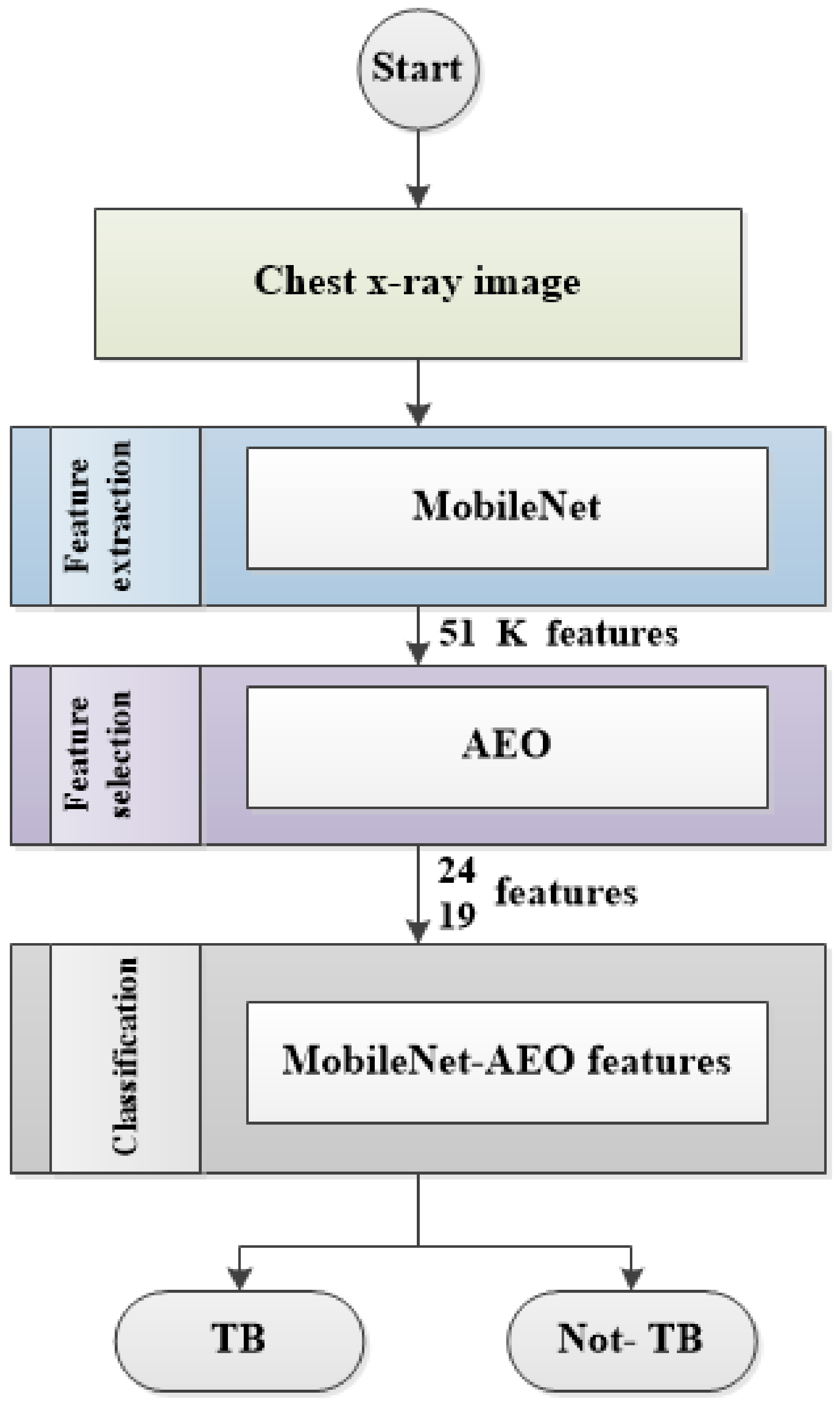
3. Proposed MobileNet-AEO for Chest X-ray Classification Approach
4. Datasets and Evaluation
4.1. Dataset Description
4.2. Evaluation
4.3. Implementation Environment
5. Results and Discussion
5.1. Parameters
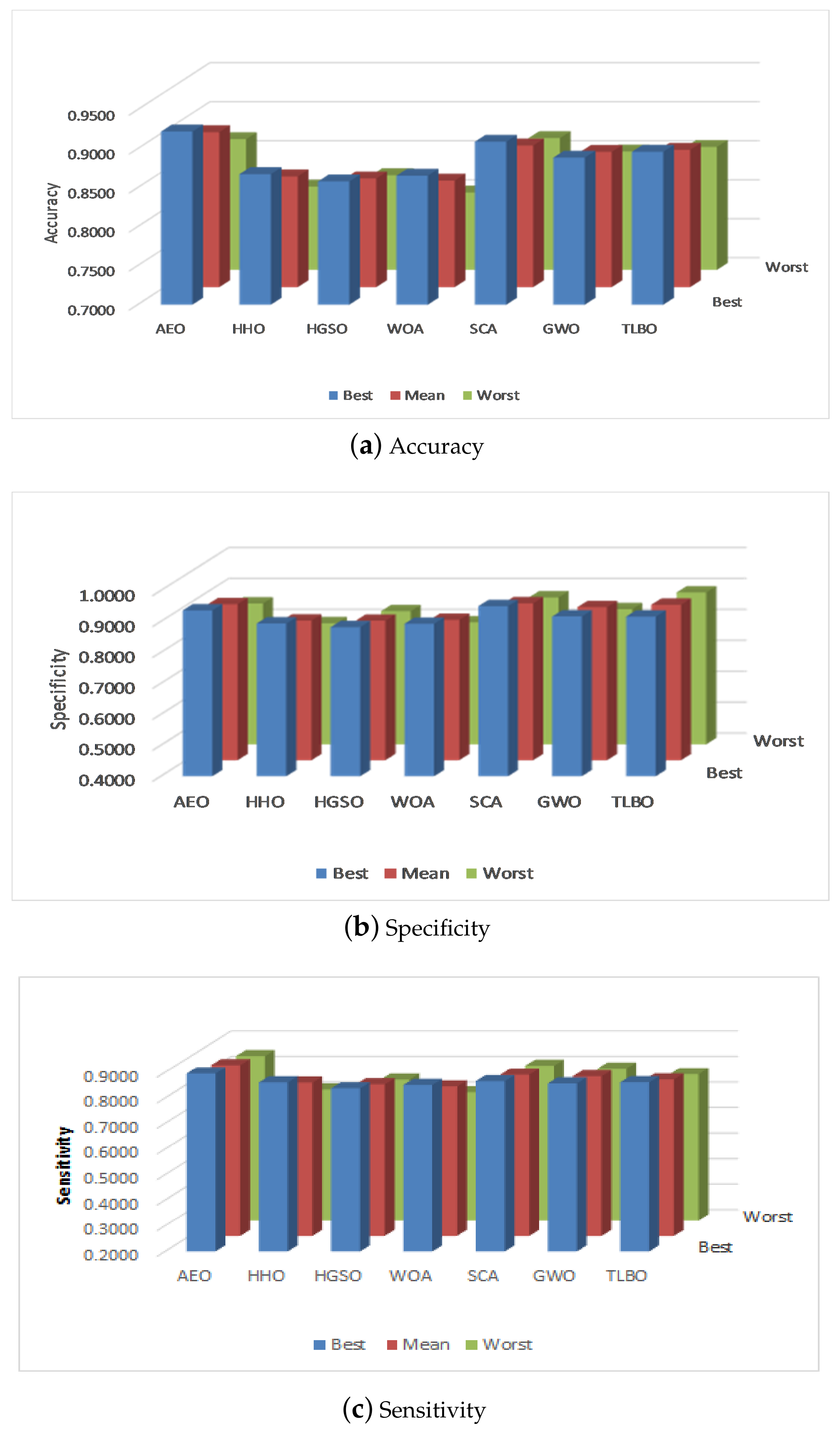
5.2. Performance
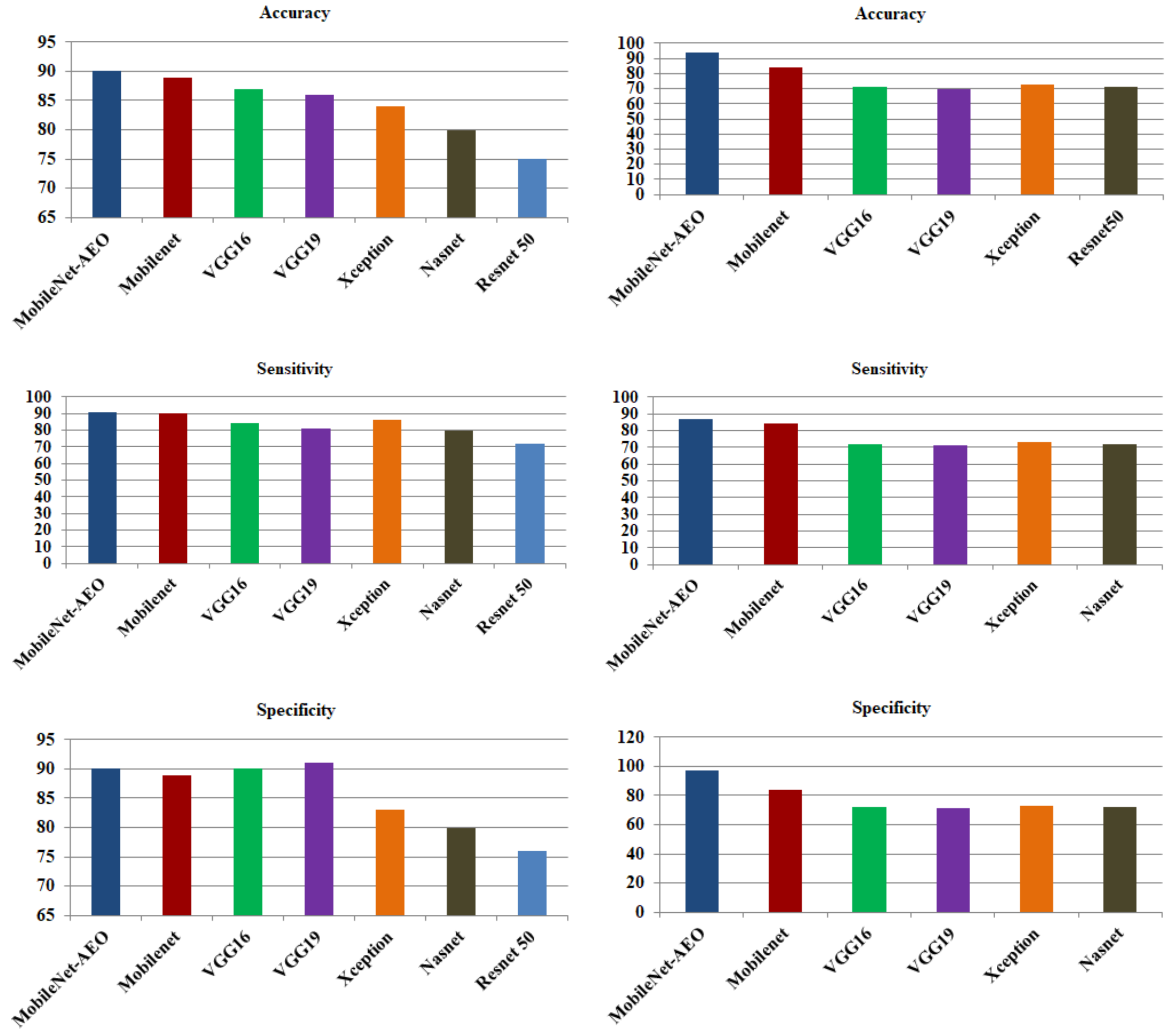
5.3. Comparison with Other CNN Models
5.4. Comparison with Related Works
6. Conclusions
Author Contributions
Funding
Conflicts of Interest
References
- Pasa, F.; Golkov, V.; Pfeiffer, F.; Cremers, D.; Pfeiffer, D. Efficient Deep Network Architectures for Fast Chest X-Ray Tuberculosis Screening and Visualization. Sci. Rep. 2019, 9, 6268. [Google Scholar] [CrossRef] [PubMed] [Green Version]
- Anderson, L.; Dean, A.; Falzon, D.; Floyd, K.; Baena, I.; Gilpin, C.; Glaziou, P.; Hamada, Y.; Hiatt, T.; Char, A.; et al. Global tuberculosis report 2015. WHO Libr. Cat. Data 2015, 1, 1689–1699. [Google Scholar]
- Sui, Y.; Wei, Y.; Zhao, D. Computer-Aided Lung Nodule Recognition by SVM Classifier Based on Combination of Random Undersampling and SMOTE. Comput. Math. Methods Med. 2015, 2015, 1–13. [Google Scholar] [CrossRef] [PubMed]
- Santosh, K.C.; Antani, S. Automated Chest X-Ray Screening: Can Lung Region Symmetry Help Detect Pulmonary Abnormalities? IEEE Trans. Med. Imaging 2018, 37, 1168–1177. [Google Scholar] [CrossRef] [PubMed]
- Khan, M.A.; Rubab, S.; Kashif, A.; Sharif, M.I.; Muhammad, N.; Shah, J.H.; Zhang, Y.D.; Satapathy, S.C. Lungs cancer classification from CT images: An integrated design of contrast based classical features fusion and selection. Pattern Recognit. Lett. 2020, 129, 77–85. [Google Scholar] [CrossRef]
- Filho, P.; Barros, A.; Ramalho, G.; Pereira, C.; Papa, J.; de Albuquerque, V.; Tavares, J. Automated recognition of lung diseases in CT images based on the optimum-path forest classifier. Neural Comput. Appl. 2019, 31, 901–914. [Google Scholar] [CrossRef]
- Woźniak, M.; Połap, D. Bio-inspired methods modeled for respiratory disease detection from medical images. Swarm Evol. Comput. 2018, 41, 69–96. [Google Scholar] [CrossRef]
- Gupta, N.; Gupta, D.; Khanna, A.; Rebouças Filho, P.; de Albuquerque, V. Evolutionary algorithms for automatic lung disease detection. Meas. J. Int. Meas. Confed. 2019, 140, 590–608. [Google Scholar] [CrossRef]
- Połap, D.; Woźniak, M.; Damaševičius, R.; Wei, W. Chest radiographs segmentation by the use of nature-inspired algorithm for lung disease detection. In Proceedings of the 2018 IEEE Symposium Series on Computational Intelligence (SSCI), Bangalore, India, 18–21 November 2018; pp. 2298–2303. [Google Scholar] [CrossRef]
- Abiyev, R.; Ma’aitah, M. Deep Convolutional Neural Networks for Chest Diseases Detection. J. Healthc. Eng. 2018, 2018. [Google Scholar] [CrossRef] [Green Version]
- Hosny, A.; Parmar, C.; Quackenbush, J.; Schwartz, L.; Aerts, H. Artificial intelligence in radiology. Nat. Rev. Cancer 2018, 18, 500–510. [Google Scholar] [CrossRef]
- Litjens, G.; Kooi, T.; Bejnordi, B.E.; Setio, A.A.A.; Ciompi, F.; Ghafoorian, M.; Van Der Laak, J.A.; Van Ginneken, B.; Sánchez, C.I. A survey on deep learning in medical image analysis. Med. Image Anal. 2017, 42, 60–88. [Google Scholar] [CrossRef] [PubMed] [Green Version]
- Rouhi, R.; Jafari, M.; Kasaei, S.; Keshavarzian, P. Benign and malignant breast tumors classification based on region growing and CNN segmentation. Expert Syst. Appl. 2015, 42, 990–1002. [Google Scholar] [CrossRef]
- Woźniak, M.; Połap, D.; Capizzi, G.; Sciuto, G.; Kośmider, L.; Frankiewicz, K. Small lung nodules detection based on local variance analysis and probabilistic neural network. Comput. Methods Programs Biomed. 2018, 161, 173–180. [Google Scholar] [CrossRef] [PubMed]
- Chouhan, V.; Singh, S.; Khamparia, A.; Gupta, D.; Tiwari, P.; Moreira, C.; Damaševičius, R.; de Albuquerque, V. A novel transfer learning based approach for pneumonia detection in chest X-ray images. Appl. Sci. 2020, 10, 559. [Google Scholar] [CrossRef] [Green Version]
- Melendez, J.; Sánchez, C.I.; Philipsen, R.H.; Maduskar, P.; Dawson, R.; Theron, G.; Dheda, K.; Van Ginneken, B. An automated tuberculosis screening strategy combining X-ray-based computer-aided detection and clinical information. Sci. Rep. 2016, 6, 25265. [Google Scholar] [CrossRef]
- Jaeger, S.; Karargyris, A.; Candemir, S.; Folio, L.; Siegelman, J.; Callaghan, F.; Xue, Z.; Palaniappan, K.; Singh, R.K.; Antani, S.; et al. Automatic tuberculosis screening using chest radiographs. IEEE Trans. Med. Imaging 2013, 33, 233–245. [Google Scholar] [CrossRef]
- Lopes, U.; Valiati, J.F. Pre-trained convolutional neural networks as feature extractors for tuberculosis detection. Comput. Biol. Med. 2017, 89, 135–143. [Google Scholar] [CrossRef]
- Vajda, S.; Karargyris, A.; Jaeger, S.; Santosh, K.; Candemir, S.; Xue, Z.; Antani, S.; Thoma, G. Feature selection for automatic tuberculosis screening in frontal chest radiographs. J. Med. Syst. 2018, 42, 146. [Google Scholar] [CrossRef]
- Lakhani, P.; Sundaram, B. Deep learning at chest radiography: Automated classification of pulmonary tuberculosis by using convolutional neural networks. Radiology 2017, 284, 574–582. [Google Scholar] [CrossRef]
- Hwang, S.; Kim, H.E.; Jeong, J.; Kim, H.J. A novel approach for tuberculosis screening based on deep convolutional neural networks. In SPIE Medical Imaging, Proceedings of the Medical Imaging 2016: Computer-Aided Diagnosis, San Diego, CA, USA, 27 February–3 March 2016; International Society for Optics and Photonics: Bellingham, WA, USA, 2016; Volume 9785, p. 97852W. [Google Scholar]
- Islam, M.T.; Aowal, M.A.; Minhaz, A.T.; Ashraf, K. Abnormality detection and localization in chest X-rays using deep convolutional neural networks. arXiv 2017, arXiv:1705.09850. [Google Scholar]
- Shin, H.C.; Roberts, K.; Lu, L.; Demner-Fushman, D.; Yao, J.; Summers, R.M. Learning to read chest x-rays: Recurrent neural cascade model for automated image annotation. In Proceedings of the IEEE Conference on Computer Vision and Pattern Recognition, Las Vegas, NV, USA, 27–30 June 2016; pp. 2497–2506. [Google Scholar]
- Deng, J.; Dong, W.; Socher, R.; Li, L.J.; Li, K.; Fei-Fei, L. Imagenet: A large-scale hierarchical image database. In Proceedings of the 2009 IEEE Conference on Computer Vision and Pattern Recognition, Miami, FL, USA, 20–25 June 2009; pp. 248–255. [Google Scholar]
- Shin, H.C.; Roth, H.R.; Gao, M.; Lu, L.; Xu, Z.; Nogues, I.; Yao, J.; Mollura, D.; Summers, R.M. Deep convolutional neural networks for computer-aided detection: CNN architectures, dataset characteristics and transfer learning. IEEE Trans. Med. Imaging 2016, 35, 1285–1298. [Google Scholar] [CrossRef] [PubMed] [Green Version]
- Ho, T.K.K.; Gwak, J. Multiple feature integration for classification of thoracic disease in chest radiography. Appl. Sci. 2019, 9, 4130. [Google Scholar] [CrossRef] [Green Version]
- Abdeldaim, A.M.; Sahlol, A.T.; Elhoseny, M.; Hassanien, A.E. Computer-aided acute lymphoblastic leukemia diagnosis system based on image analysis. In Advances in Soft Computing and Machine Learning in Image Processing; Springer: Berlin, Germany, 2018; pp. 131–147. [Google Scholar]
- Sahlol, A.T.; Abdeldaim, A.M.; Hassanien, A.E. Automatic acute lymphoblastic leukemia classification model using social spider optimization algorithm. In Soft Computing; Springer: Berlin, Germany, 2018; pp. 1–16. [Google Scholar]
- Ke, Q.; Zhang, J.; Wei, W.; Połap, D.; Woźniak, M.; Kośmider, L.; Damaševičius, R. A neuro-heuristic approach for recognition of lung diseases from X-ray images. Expert Syst. Appl. 2019, 126, 218–232. [Google Scholar] [CrossRef]
- Qi, G.; Luo, J. Small Data Challenges in Big Data Era: A Survey of Recent Progress on Unsupervised and Semi-Supervised Methods. arXiv 2019, arXiv:1903.11260. [Google Scholar]
- Sharif Razavian, A.; Azizpour, H.; Sullivan, J.; Carlsson, S. CNN features off-the-shelf: An astounding baseline for recognition. In Proceedings of the IEEE Conference on Computer Vision and Pattern Recognition Workshops, Columbus, OH, USA, 23–28 June 2014; pp. 806–813. [Google Scholar]
- Donahue, J.; Jia, Y.; Vinyals, O.; Hoffman, J.; Zhang, N.; Tzeng, E.; Darrell, T. Decaf: A deep convolutional activation feature for generic visual recognition. In Proceedings of the International Conference on Machine Learning, Beijing, China, 21–26 June 2014; pp. 647–655. [Google Scholar]
- Nguyen, L.D.; Lin, D.; Lin, Z.; Cao, J. Deep CNNs for microscopic image classification by exploiting transfer learning and feature concatenation. In Proceedings of the 2018 IEEE International Symposium on Circuits and Systems (ISCAS), Florence, Italy, 27–30 May 2018; pp. 1–5. [Google Scholar]
- Simonyan, K.; Zisserman, A. Very deep convolutional networks for large-scale image recognition. arXiv 2014, arXiv:1409.1556. [Google Scholar]
- He, K.; Zhang, X.; Ren, S.; Sun, J. Deep residual learning for image recognition. In Proceedings of the IEEE Conference on Computer Vision and Pattern Recognition, Las Vegas, NV, USA, 27–30 June 2016; pp. 770–778. [Google Scholar]
- Blog, G. AutoML for Large Scale Image Classification and Object Detection. 2017. Available online: https://research.googleblog.com/2017/11/automl-for-large-scaleimage.html (accessed on 31 May 2020).
- Howard, A.G.; Zhu, M.; Chen, B.; Kalenichenko, D.; Wang, W.; Weyand, T.; Andreetto, M.; Adam, H. Mobilenets: Efficient convolutional neural networks for mobile vision applications. arXiv 2017, arXiv:1704.04861. [Google Scholar]
- Szegedy, C.; Liu, W.; Jia, Y.; Sermanet, P.; Reed, S.; Anguelov, D.; Erhan, D.; Vanhoucke, V.; Rabinovich, A. Going deeper with convolutions. In Proceedings of the IEEE Conference on Computer Vision and Pattern Recognition, Boston, MA, USA, 7–12 June 2015; pp. 1–9. [Google Scholar]
- Chollet, F. Xception: Deep learning with depthwise separable convolutions. In Proceedings of the IEEE Conference on Computer Vision and Pattern Recognition, Honolulu, HI, USA, 21–26 July 2017; pp. 1251–1258. [Google Scholar]
- Li, Z.; Wang, C.; Han, M.; Xue, Y.; Wei, W.; Li, L.J.; Fei-Fei, L. Thoracic disease identification and localization with limited supervision. In Proceedings of the IEEE Conference on Computer Vision and Pattern Recognition, Salt Palace Convention Cetner, Salt Lake City, UT, USA, 28–23 June 2018; pp. 8290–8299. [Google Scholar]
- Zhao, W.; Wang, L.; Zhang, Z. Artificial ecosystem-based optimization: A novel nature-inspired meta-heuristic algorithm. Neural Comput. Appl. 2019. [Google Scholar] [CrossRef]
- Ioffe, S.; Szegedy, C. Batch normalization: Accelerating deep network training by reducing internal covariate shift. arXiv 2015, arXiv:1502.03167. [Google Scholar]
- Bengio, Y.; Courville, A.; Vincent, P. Representation learning: A review and new perspectives. IEEE Trans. Pattern Anal. Mach. Intell. 2013, 35, 1798–1828. [Google Scholar] [CrossRef]
- Bolboacă, S.D.; Jäntschi, L.; Sestraş, A.F.; Sestraş, R.E.; Pamfil, D.C. Pearson-Fisher chi-square statistic revisited. Information 2011, 2, 528–545. [Google Scholar] [CrossRef] [Green Version]
- Sahlol, A.T.; Kollmannsberger, P.; Ewees, A.A. Efficient Classification of White Blood Cell Leukemia with Improved Swarm Optimization of Deep Features. Sci. Rep. 2020, 10, 1–11. [Google Scholar] [CrossRef]
- Bálint, D.; Jäntschi, L. Missing data calculation using the antioxidant activity in selected herbs. Symmetry 2019, 11, 779. [Google Scholar] [CrossRef] [Green Version]
- Jaeger, S.; Candemir, S.; Antani, S.; Wáng, Y.X.J.; Lu, P.X.; Thoma, G. Two public chest X-ray datasets for computer-aided screening of pulmonary diseases. Quant. Imaging Med. Surg. 2014, 4, 475–477. [Google Scholar] [PubMed]
- Kermany, D.S.; Goldbaum, M.; Cai, W.; Valentim, C.C.; Liang, H.; Baxter, S.L.; McKeown, A.; Yang, G.; Wu, X.; Yan, F.; et al. Identifying medical diagnoses and treatable diseases by image-based deep learning. Cell 2018, 172, 1122–1131. [Google Scholar] [CrossRef] [PubMed]
- Zhu, W.; Zeng, N.; Wang, N. Sensitivity, specificity, accuracy, associated confidence interval and ROC analysis with practical SAS implementations. NESUG Proc. 2010, 19, 67. [Google Scholar]
- Bisong, E. Building Machine Learning and Deep Learning Models on Google Cloud Platform; Springer: Berlin, Germany, 2019. [Google Scholar]
- Chollet, F. Keras. 2015. Available online: https://github.com/fchollet/keras (accessed on 31 May 2020).
- Abadi, M.; Agarwal, A.; Barham, P.; Brevdo, E.; Chen, Z.; Citro, C.; Corrado, G.S.; Davis, A.; Dean, J.; Devin, M.; et al. TensorFlow: Large-Scale Machine Learning on Heterogeneous Systems. 2015. Available online: https://tensorflow.org (accessed on 31 May 2020).
- Wichrowska, O.; Maheswaranathan, N.; Hoffman, M.W.; Colmenarejo, S.G.; Denil, M.; de Freitas, N.; Sohl-Dickstein, J. Learned optimizers that scale and generalize. In Proceedings of the 34th International Conference on Machine Learning, Sydney, Australia, 6–11 August 2017; Volume 70, pp. 3751–3760. [Google Scholar]
- Heidari, A.A.; Mirjalili, S.; Faris, H.; Aljarah, I.; Mafarja, M.; Chen, H. Harris hawks optimization: Algorithm and applications. Future Gener. Comput. Syst. 2019, 97, 849–872. [Google Scholar] [CrossRef]
- Hashim, F.A.; Houssein, E.H.; Mabrouk, M.S.; Al-Atabany, W.; Mirjalili, S. Henry gas solubility optimization: A novel physics-based algorithm. Future Gener. Comput. Syst. 2019, 101, 646–667. [Google Scholar] [CrossRef]
- Mirjalili, S.; Lewis, A. The whale optimization algorithm. Adv. Eng. Softw. 2016, 95, 51–67. [Google Scholar] [CrossRef]
- Ibrahim, R.A.; Elaziz, M.A.; Lu, S. Chaotic opposition-based grey-wolf optimization algorithm based on differential evolution and disruption operator for global optimization. Expert Syst. Appl. 2018, 108, 1–27. [Google Scholar] [CrossRef]
- Elaziz, M.A.; Oliva, D.; Xiong, S. An improved opposition-based sine cosine algorithm for global optimization. Expert Syst. Appl. 2017, 90, 484–500. [Google Scholar] [CrossRef]
- Allam, M.; Nandhini, M. Optimal feature selection using binary teaching learning based optimization algorithm. J. King Saud Univ. Comput. Inf. Sci. 2018. [Google Scholar] [CrossRef]
- Sivaramakrishnan, R.; Antani, S.; Candemir, S.; Xue, Z.; Abuya, J.; Kohli, M.; Alderson, P.; Thoma, G. Comparing deep learning models for population screening using chest radiography. In SPIE Medical Imaging, Proceedings of the Medical Imaging 2018: Computer-Aided Diagnosis, Houston, TX, USA, 10–15 February 2018; International Society for Optics and Photonics: Bellingham, WA, USA, 2018; Volume 10575, p. 105751E. [Google Scholar]
- Rajaraman, S.; Candemir, S.; Kim, I.; Thoma, G.; Antani, S. Visualization and interpretation of convolutional neural network predictions in detecting pneumonia in pediatric chest radiographs. Appl. Sci. 2018, 8, 1715. [Google Scholar] [CrossRef] [PubMed] [Green Version]


| Dataset 2 |  |  |  |  |  |
| Shenzhen |  |  |  |  |  |
| AEO | HHO | HGSO | WOA | SCA | GWO | TLBO | ||
|---|---|---|---|---|---|---|---|---|
| Acc | Best | 0.9023 | 0.8195 | 0.8120 | 0.8120 | 0.8872 | 0.8421 | 0.8872 |
| Mean | 0.8617 | 0.7880 | 0.7835 | 0.7744 | 0.8436 | 0.8150 | 0.8526 | |
| Worst | 0.8045 | 0.7368 | 0.7669 | 0.7293 | 0.8271 | 0.7744 | 0.8195 | |
| STD | 0.0400 | 0.0374 | 0.0171 | 0.0340 | 0.0252 | 0.0294 | 0.0253 | |
| Sens | Best | 0.9194 | 0.8923 | 0.8448 | 0.8636 | 0.8676 | 0.8500 | 0.9077 |
| Mean | 0.8839 | 0.8092 | 0.8069 | 0.7848 | 0.8294 | 0.8033 | 0.8369 | |
| Worst | 0.8548 | 0.7231 | 0.7759 | 0.7273 | 0.8088 | 0.7667 | 0.7846 | |
| STD | 0.0239 | 0.0612 | 0.0256 | 0.0540 | 0.0246 | 0.0361 | 0.0456 | |
| Spec | Best | 0.9014 | 0.8382 | 0.8133 | 0.8358 | 0.9385 | 0.8630 | 0.8824 |
| Mean | 0.8423 | 0.7676 | 0.7653 | 0.7642 | 0.8585 | 0.8247 | 0.8676 | |
| Worst | 0.7465 | 0.6765 | 0.7333 | 0.6567 | 0.8000 | 0.7123 | 0.8529 | |
| STD | 0.0609 | 0.0627 | 0.0335 | 0.0711 | 0.0503 | 0.0653 | 0.0104 |
| AEO | HHO | HGSO | WOA | SCA | GWO | TLBO | ||
|---|---|---|---|---|---|---|---|---|
| Acc | Best | 0.9418 | 0.9152 | 0.9041 | 0.9187 | 0.9307 | 0.9349 | 0.9050 |
| Mean | 0.9360 | 0.8964 | 0.8955 | 0.8991 | 0.9199 | 0.9322 | 0.8997 | |
| Worst | 0.9307 | 0.8767 | 0.8759 | 0.8690 | 0.9110 | 0.9289 | 0.8955 | |
| STD | 0.0048 | 0.0153 | 0.0116 | 0.0189 | 0.0081 | 0.0022 | 0.0038 | |
| Sens | Best | 0.8722 | 0.8291 | 0.8306 | 0.8384 | 0.8630 | 0.8642 | 0.8148 |
| Mean | 0.8518 | 0.7905 | 0.7792 | 0.7848 | 0.8327 | 0.8463 | 0.7872 | |
| Worst | 0.8307 | 0.7025 | 0.7264 | 0.6768 | 0.8017 | 0.8210 | 0.7609 | |
| STD | 0.0174 | 0.0538 | 0.0393 | 0.0632 | 0.0247 | 0.0183 | 0.0191 | |
| Spec | Best | 0.9708 | 0.9495 | 0.9501 | 0.9500 | 0.9612 | 0.9704 | 0.9495 |
| Mean | 0.9668 | 0.9357 | 0.9370 | 0.9438 | 0.9561 | 0.9652 | 0.9380 | |
| Worst | 0.9637 | 0.9061 | 0.9268 | 0.9310 | 0.9491 | 0.9609 | 0.9288 | |
| STD | 0.0027 | 0.0178 | 0.0094 | 0.0075 | 0.0054 | 0.0043 | 0.0091 |
| AEO | HHO | HGSO | WOA | SCA | GWO | TLBO | ||
|---|---|---|---|---|---|---|---|---|
| Dataset1 | Features | 24.6 | 9.6 | 11.6 | 10.8 | 42.2 | 58.8 | 19.6 |
| Best time (s) | 8.8713 | 9.1562 | 8.1690 | 4.1322 | 5.1606 | 9.0793 | 9.1075 | |
| Mean time (s) | 9.7251 | 9.6065 | 8.5953 | 4.3891 | 5.2591 | 9.5839 | 9.5879 | |
| STD time (s) | 0.9068 | 0.3497 | 0.2658 | 0.1653 | 0.0912 | 0.3606 | 0.4349 | |
| Dataset2 | Features | 19 | 33.8 | 31.6 | 52.6 | 31.8 | 72 | 30.8 |
| Best time (s) | 137.7945 | 250.7114 | 671.3892 | 125.0128 | 251.9918 | 422.1539 | 247.6316 | |
| Mean time (s) | 162.4733 | 281.7812 | 743.5204 | 128.3362 | 257.9852 | 467.4882 | 297.0471 | |
| STD time (s) | 7.9267 | 30.0768 | 50.8346 | 2.2845 | 9.4944 | 26.7742 | 33.5236 |
| Shenzhen | Features | Percentage | Accuracy | Specificity | Sensitivity |
|---|---|---|---|---|---|
| MobileNet | 50176 | 100% | 0.89 | 0.89 | 0.90 |
| Proposed approach | ∼25 | 0.05% | 0.902 | 0.901 | 0.914 |
| Dataset 2 | Features | Percentage | Accuracy | Specificity | Sensitivity |
| MobileNet | 50176 | 100% | 0.842 | 0.846 | 0.846 |
| Proposed approach | 19 | 0.038% | 0.941 | 0.97 | 0.872 |
| Shenzhen Dataset | Feature Extraction | Classifier | Accuracy (%) |
|---|---|---|---|
| Jaeger et al. [17] | Manually | SVM | 84.10 |
| Hwang et al. [21] | Deep features by CNN | KNN | 83.70 |
| Lopes et al. [18] | ResNet, VGG and GoogLeNet | SVM | 84.60 |
| Sivaramakrishnan et al. [60] | VGG16 with optimal features | CNN | 85.5 |
| Proposed approach | Deep features by MobileNet, feature selection by AEO | CNN | 90.2 |
| Dataset 2 | Feature extraction | Classifier | Accuracy (%) |
| Kermany et al. [48] | Deep features | N/A | 92.8 |
| Rajaraman et al. [61] | Deep features by CNN architectures | Residual CNN | 91 |
| Inception | 88.6 | ||
| Proposed approach | Deep features by MobileNet, feature selection by AEO | CNN | 94.1 |
© 2020 by the authors. Licensee MDPI, Basel, Switzerland. This article is an open access article distributed under the terms and conditions of the Creative Commons Attribution (CC BY) license (http://creativecommons.org/licenses/by/4.0/).
Share and Cite
Sahlol, A.T.; Abd Elaziz, M.; Tariq Jamal, A.; Damaševičius, R.; Farouk Hassan, O. A Novel Method for Detection of Tuberculosis in Chest Radiographs Using Artificial Ecosystem-Based Optimisation of Deep Neural Network Features. Symmetry 2020, 12, 1146. https://doi.org/10.3390/sym12071146
Sahlol AT, Abd Elaziz M, Tariq Jamal A, Damaševičius R, Farouk Hassan O. A Novel Method for Detection of Tuberculosis in Chest Radiographs Using Artificial Ecosystem-Based Optimisation of Deep Neural Network Features. Symmetry. 2020; 12(7):1146. https://doi.org/10.3390/sym12071146
Chicago/Turabian StyleSahlol, Ahmed T., Mohamed Abd Elaziz, Amani Tariq Jamal, Robertas Damaševičius, and Osama Farouk Hassan. 2020. "A Novel Method for Detection of Tuberculosis in Chest Radiographs Using Artificial Ecosystem-Based Optimisation of Deep Neural Network Features" Symmetry 12, no. 7: 1146. https://doi.org/10.3390/sym12071146