A Feature Selection Model for Network Intrusion Detection System Based on PSO, GWO, FFA and GA Algorithms


Abstract
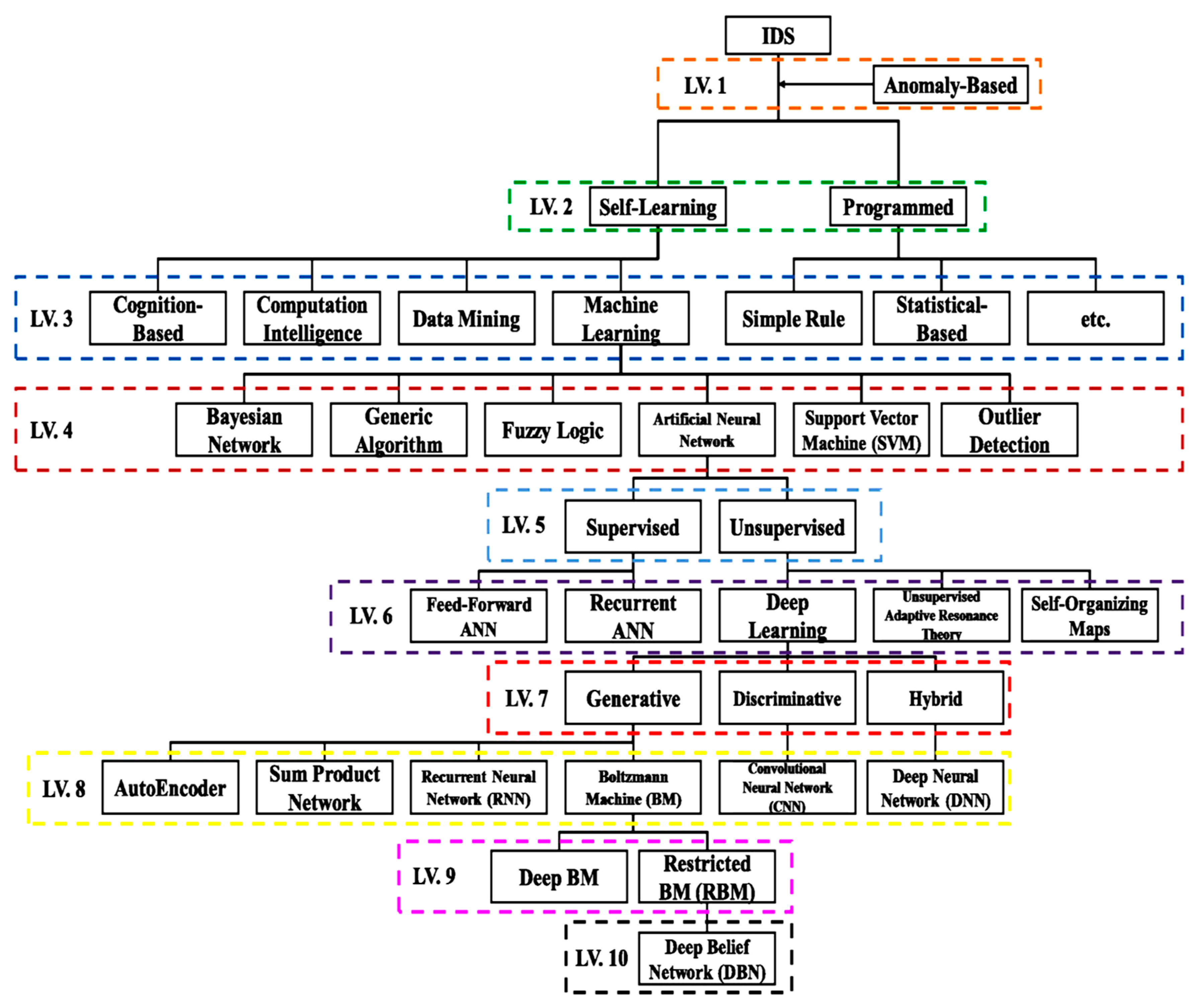
:1. Introduction
- Identify the optimal feature set that is in the UNSW-NB15 dataset. The present study aimed to do that based on the PSO, GWO, FFA and GA algorithms;
- Propose a filtering-based feature selection model for the NIDS. The present study aimed to do that based on the PSO, GWO, FFA and GA algorithms. It aimed to do that to reduce the number of the selected features;
- Determine the best combination between the PSO, GWO, FFA and GA algorithms. The present study aimed to determine that to filter the selected features that improve the performance of the detection mechanism.
2. Related Works
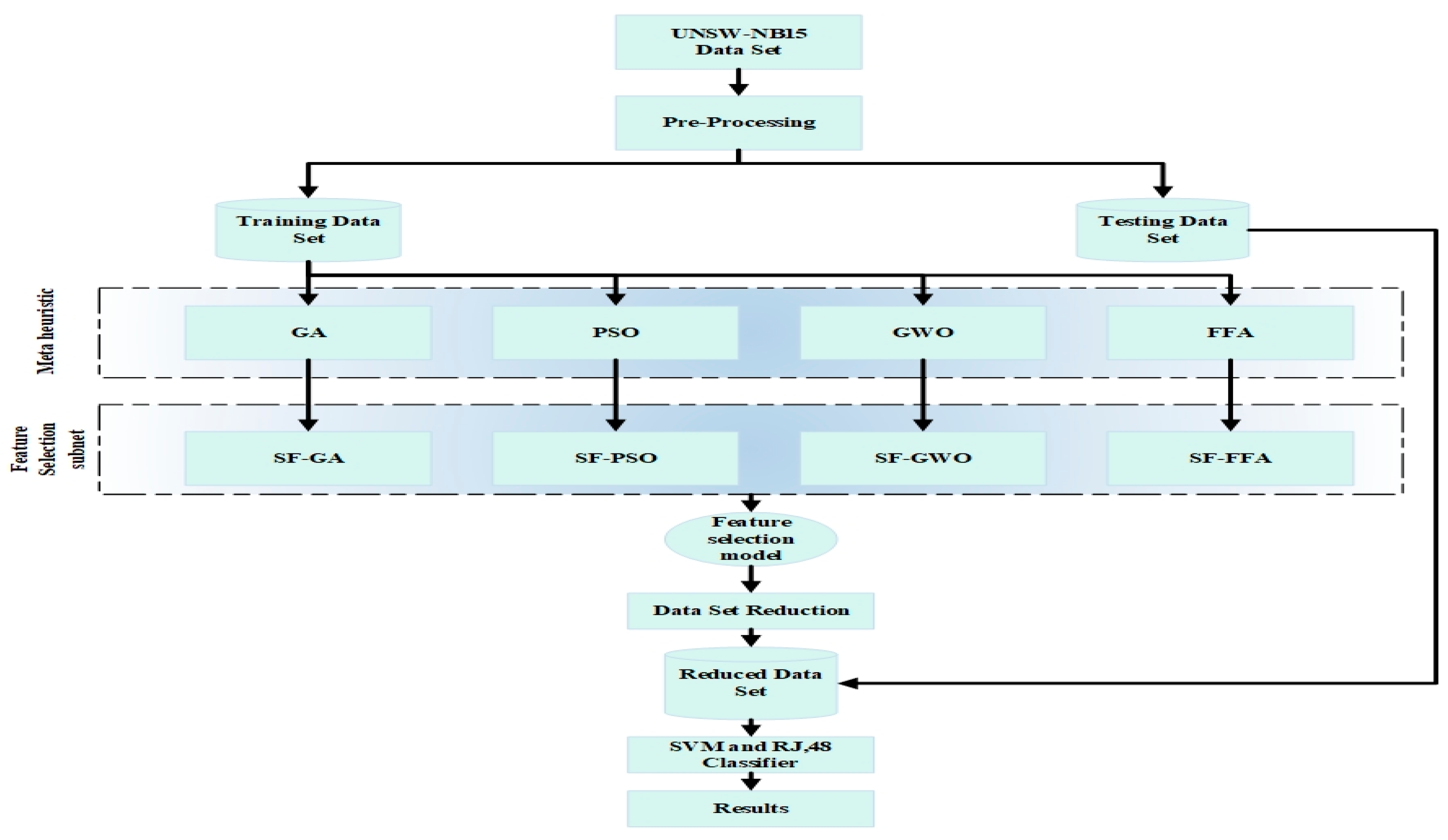
3. The Proposed Model
3.1. The Pre-Processing Stage
- A
- The removal of the labels: Each feature in the original UNSW-NB15 dataset has a label. Removing those labels is important in order to adapt the dataset with the EvoloPy-FS environment;
- B
- Removing Features: The original UNSW-NB15 dataset has 45 features. Two features of those features are class labels (attack cat and label). The attack cat cannot be considered as a feature. Thus, it is important to delete it. Deleting it is important because the main objective sought from this work is represented in reducing the features;
- C
- Label encoding: Some labels in the dataset—e.g., protocol, state and service type—are given string values. Therefore, it is very significant to have those values encoded into numerical values;
- D
- Data binarization: The numerical data in the dataset are in various ranges. During the training process, these data provide the classifier with a variety of challenges in order to compensate for such variations. Therefore, the values in each feature must be standardized. Thus, the least value in each one of the features should be 0. However, the maximum value should be 1. It makes the classifier more homogeneous. It preserves the difference between the values of each feature.
3.2. The Selection of Features Based on the Bio-Inspired Metaheuristic Algorithms
3.2.1. GA Features Selection
3.2.2. PSO Features Selection
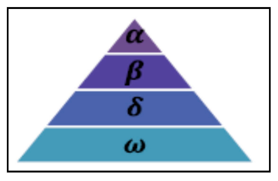
3.2.3. GWO Features Selection
- (1)
- Tracking the prey and chasing and approaching it;
- (2)
- Pursuing the prey and encircling and harassing it to stop its movement;
- (3)
- Launching an attack against the prey being attacked. The algorithm mimics the whole described hierarchy and group hunting procedures. It mimics those procedures to solve complex engineering problems.
3.2.4. FFA Features Selection
- (a)
- Regarding all the fireflies, they are unisex;
- (b)
- The brightness of the fireflies is proportional to their attractiveness;
- (c)
- The firefly’s brightness is determined and influenced by the environment of the objective functions. In terms of the maximization problem, the brightness may be proportional to the value of the objective function.
3.3. Feature Selection Model Based on MI
- Selected feature set based on PSO (S1);
- Selected feature set based on GWO (S2);
- Selected feature set based on FFA (S3);
- Selected feature set based on GA (S4).
3.4. Machine Learning Classifiers
3.4.1. SVM Classifier
3.4.2. J48 (C4.5 Decision Tree) Classifier
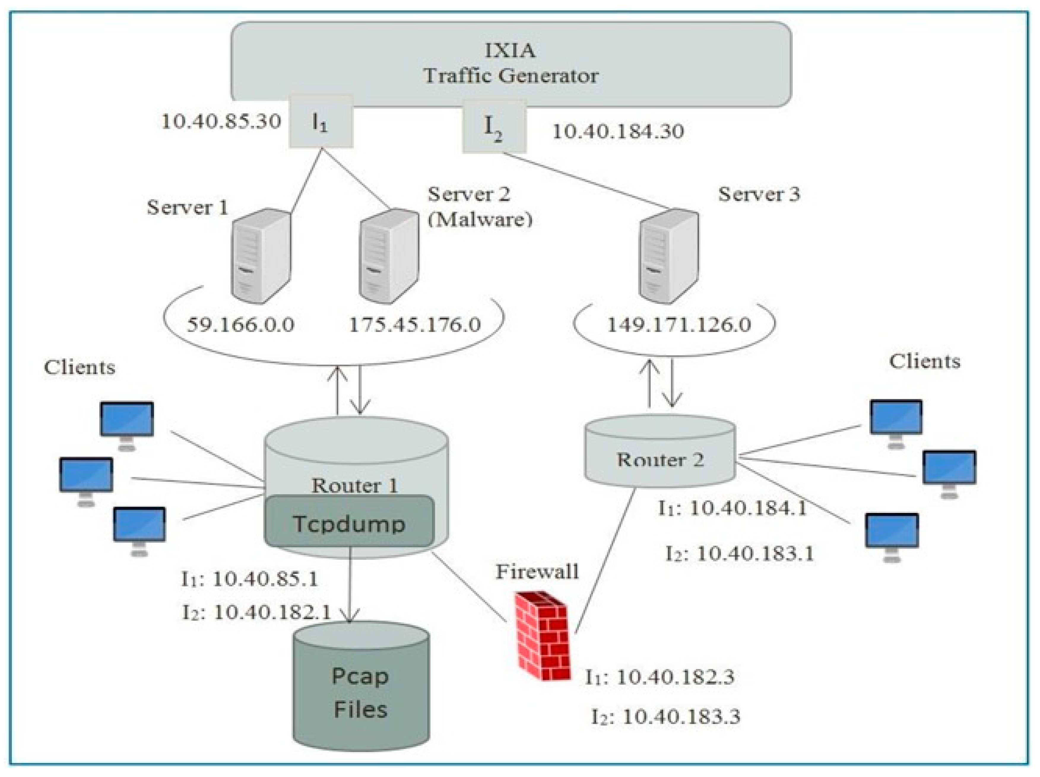
4. Dataset Description
5. Performance Evaluation Metrics
6. Results and Discussion
6.1. Selected Feature Experiments Results
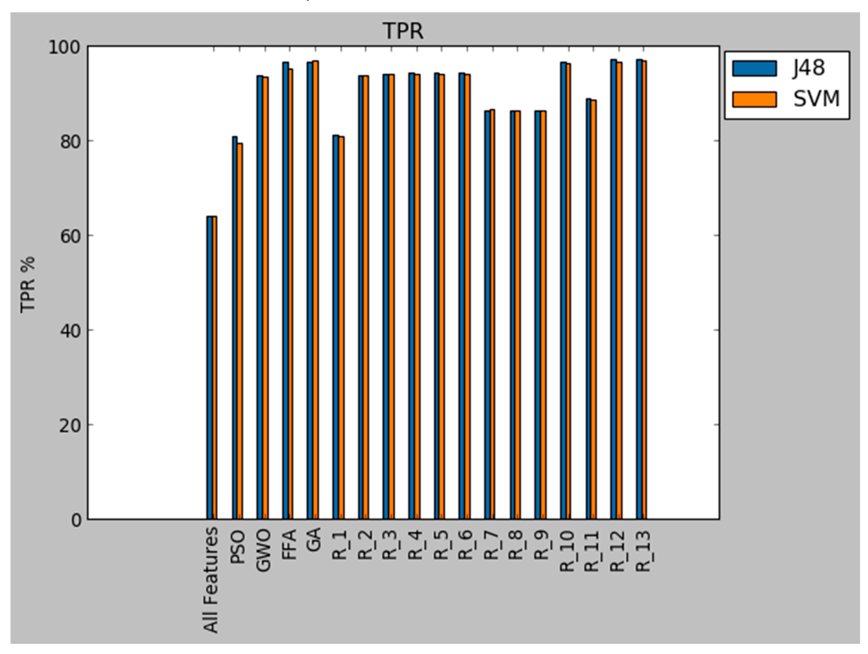
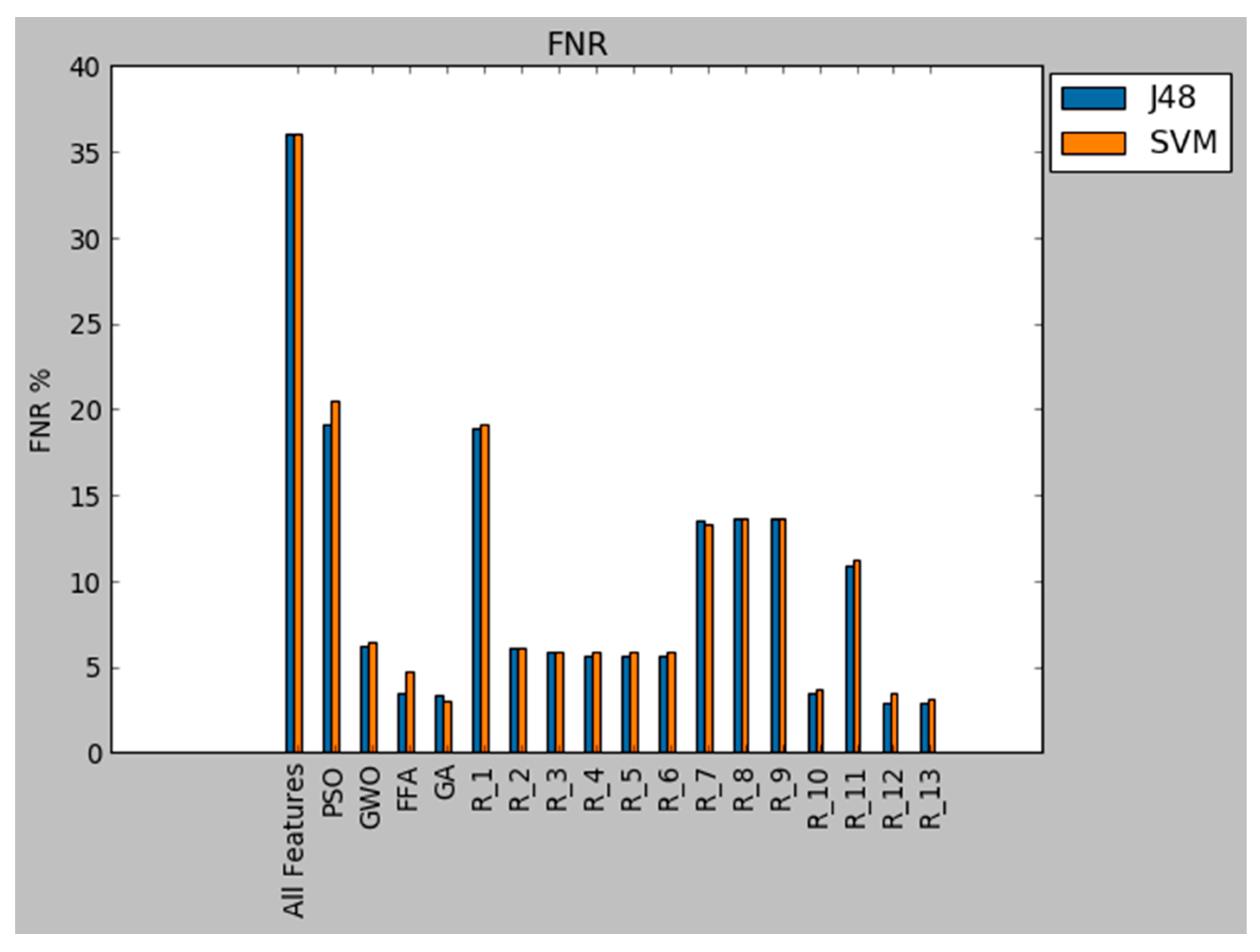
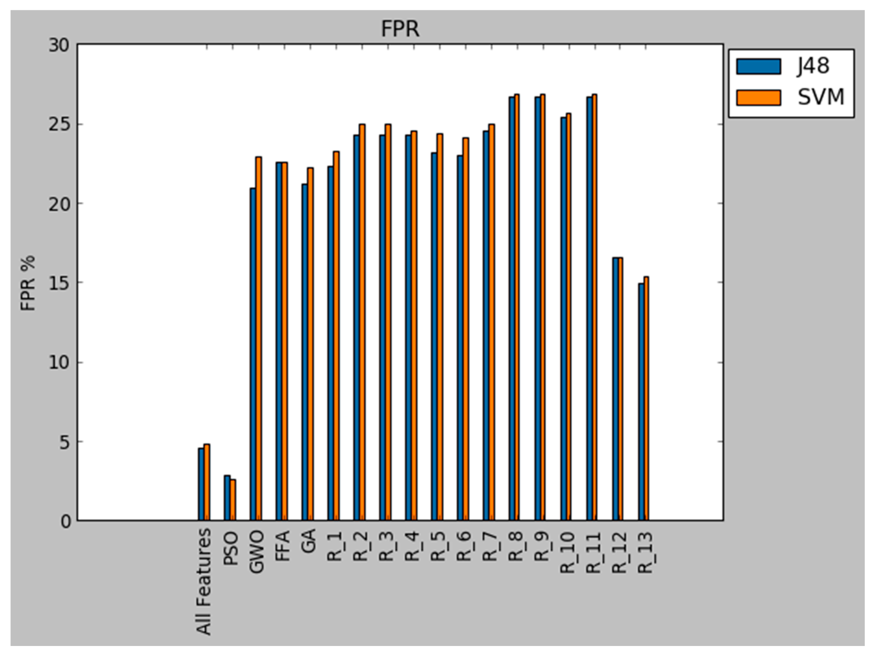
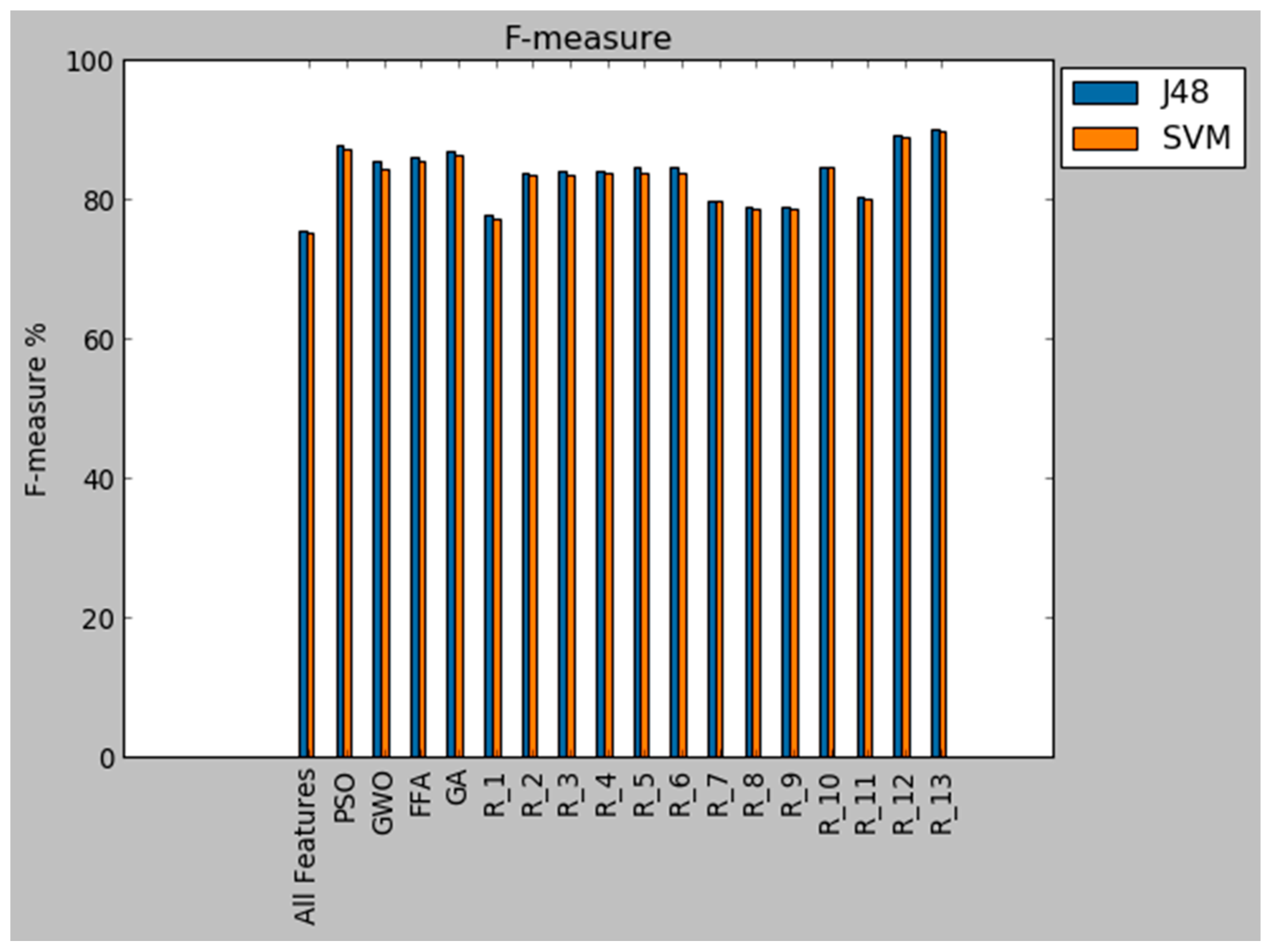
6.2. Experimental Evaluation Results
7. Conclusions
Funding
Conflicts of Interest
References
- Vinchurkar, D.P.; Reshamwala, A. A Review of Intrusion Detection System Using Neural Network and Machine Learning. J. Eng. Sci. Innov. Technol. 2012, 1, 54–63. [Google Scholar]
- Othman, S.M.; Alsohybe, N.T.; Ba-Alwi, F.M.; Zahary, A.T. Survey on Intrusion Detection System Types. Int. J. Cyber Secur. Digit. Forensics 2018, 7, 444–463. [Google Scholar]
- Zarpelão, B.B.; Miani, R.S.; Kawakani, C.T.; de Alvarenga, S.C. A survey of intrusion detection in Internet of Things. J. Netw. Comput. Appl. 2017, 84, 25–37. [Google Scholar] [CrossRef]
- Kwon, D.; Kim, H.; Kim, J.; Suh, S.C.; Kim, I.; Kim, K.J. A survey of deep learning-based network anomaly detection. Clust. Comput. 2017, 22, 1–13. [Google Scholar] [CrossRef]
- Win, T.Z.; Kham, N.S.M. Information Gain Measured Feature Selection to Reduce High Dimensional Data. In Proceedings of the 17th International Conference on Computer Applications (ICCA 2019), Novotel hotel, Yangon, Myanmar, 27 February–1 March 2019; pp. 68–73. [Google Scholar]
- Liu, H.; Motoda, H. Feature Selection for Knowledge Discovery and Data Mining; Springer Science & Business Media: Berlin/Heidelberg, Germany, 2012; Volume 454. [Google Scholar]
- Al-Tashi, Q.; Rais, H.M.; Abdulkadir, S.J.; Mirjalili, S.; Alhussian, H. A Review of Grey Wolf Optimizer-Based Feature Selection Methods for Classification. In Evolutionary Machine Learning Techniques; Springer: Berlin/Heidelberg, Germany, 2020; pp. 273–286. [Google Scholar]
- Emary, E.; Zawbaa, H.M.; Hassanien, A.E. Binary grey wolf optimization approaches for feature selection. Neurocomputing 2016, 172, 371–381. [Google Scholar] [CrossRef]
- Al-Tashi, Q.; Kadir, S.J.A.; Rais, H.M.; Mirjalili, S.; Alhussian, H. Binary optimization using hybrid grey wolf optimization for feature selection. IEEE Access 2019, 7, 39496–39508. [Google Scholar] [CrossRef]
- Sahoo, A.; Chandra, S. Multi-objective grey wolf optimizer for improved cervix lesion classification. Appl. Soft Comput. 2017, 52, 64–80. [Google Scholar] [CrossRef]
- Mitchell, M. An Introduction to Genetic Algorithms; MIT Press: Cambridge, MA, USA, 1998. [Google Scholar]
- Gharaee, H.; Hosseinvand, H. A new feature selection IDS based on genetic algorithm and SVM. In Proceedings of the 2016 8th International Symposium on Telecommunications (IST), Tehran, Iran, 27–28 September 2016; pp. 139–144. [Google Scholar]
- Al Balas, F.; Almomani, O.; Jazoh, R.M.A.; Khamayseh, Y.M.; Saaidah, A. An Enhanced End to End Route Discovery in AODV using Multi-Objectives Genetic Algorithm. In Proceedings of the 2019 IEEE Jordan International Joint Conference on Electrical Engineering and Information Technology (JEEIT), Amman, Jordan, 9–11 April 2019; pp. 209–214. [Google Scholar]
- Marini, F.; Walczak, B. Particle swarm optimization (PSO). A tutorial. Chemom. Intell. Lab. Syst. 2015, 149, 153–165. [Google Scholar] [CrossRef]
- Srinoy, S. Intrusion detection model based on particle swarm optimization and support vector machine. In Proceedings of the 2007 IEEE Symposium on Computational Intelligence in Security and Defense Applications, Honolulu, HI, USA, 1–5 April 2007; pp. 186–192. [Google Scholar]
- Kennedy, J.; Eberhart, R. Particle swarm optimization. In Proceedings of the ICNN’95-International Conference on Neural Networks, Perth, Australia, 27 November–1 December 1995; Volume 4, pp. 1942–1948. [Google Scholar]
- Mirjalili, S.; Mirjalili, S.M.; Lewis, A. Grey Wolf Optimizer. Adv. Eng. Softw. 2014, 69, 46–61. [Google Scholar] [CrossRef] [Green Version]
- Devi, E.M.; Suganthe, R.C. Feature selection in intrusion detection grey wolf optimizer. Asian J. Res. Soc. Sci. Humanit. 2017, 7, 671–682. [Google Scholar] [CrossRef]
- Alzubi, Q.M.; Anbar, M.; Alqattan, Z.N.M.; Al-Betar, M.A.; Abdullah, R. Intrusion detection system based on a modified binary grey wolf optimisation. Neural Comput. Appl. 2019, 32, 6125–6137. [Google Scholar] [CrossRef]
- Yang, X.-S.; He, X. Firefly algorithm: Recent advances and applications. arXiv 2013, arXiv:1308.3898. [Google Scholar] [CrossRef] [Green Version]
- Selvakumar, B.; Muneeswaran, K. Firefly algorithm based feature selection for network intrusion detection. Comput. Secur. 2019, 81, 148–155. [Google Scholar]
- Hasan, M.A.M.; Nasser, M.; Pal, B.; Ahmad, S. Support vector machine and random forest modeling for intrusion detection system (IDS). J. Intell. Learn. Syst. Appl. 2014, 6, 42869. [Google Scholar] [CrossRef] [Green Version]
- Mohammad, A.H.; Alwada’n, T.; Al-Momani, O. Arabic text categorization using support vector machine, Naïve Bayes and neural network. Gstf J. Comput. 2016, 5, 108. [Google Scholar] [CrossRef]
- Madi, M.; Jarghon, F.; Fazea, Y.; Almomani, O.; Saaidah, A. Comparative analysis of classification techniques for network fault management. Turk. J. Elec. Eng. Comp. Sci. 2020, 28, 1442–1457. [Google Scholar] [CrossRef]
- Sahu, S.; Mehtre, B.M. Network intrusion detection system using J48 Decision Tree. In Proceedings of the 2015 International Conference on Advances in Computing, Communications and Informatics (ICACCI), Kochi, India, 10–13 Augest 2015; pp. 2023–2026. [Google Scholar]
- Mohammad, A.H.; Al-Momani, O.; Alwada’n, T. Arabic text categorization using k-nearest neighbour, Decision Trees (C4. 5) and Rocchio classifier: A comparative study. Int. J. Curr. Eng. Technol. 2016, 6, 477–482. [Google Scholar]
- Aslahi-Shahri, B.M.; Rahmani, R.; Chizari, M.; Maralani, A.; Eslami, M.; Golkar, M.J.; Ebrahimi, A. A hybrid method consisting of GA and SVM for intrusion detection system. Neural Comput. Appl. 2016, 27, 1669–1676. [Google Scholar] [CrossRef]
- Ahmad, I.; Abdullah, A.; Alghamdi, A.; Alnfajan, K.; Hussain, M. Intrusion detection using feature subset selection based on MLP. Sci. Res. Essays 2011, 6, 6804–6810. [Google Scholar]
- Ghanem, W.; Jantan, A. Novel multi-objective artificial bee colony optimization for wrapper based feature selection in intrusion detection. Int. J. Adv. Soft Comput. Appl. 2016, 8, 70–81. [Google Scholar]
- Zaman, S.; El-Abed, M.; Karray, F. Features selection approaches for intrusion detection systems based on evolution algorithms. In Proceedings of the 7th International Conference on Ubiquitous Information Management and Communication, Kota Kinabalu, Malaysia, 17–19 January 2013; pp. 1–5. [Google Scholar]
- Chung, Y.Y.; Wahid, N. A hybrid network intrusion detection system using simplified swarm optimization (SSO). Appl. Soft Comput. 2012, 12, 3014–3022. [Google Scholar] [CrossRef]
- Syarif, I. Feature selection of network intrusion data using genetic algorithm and particle swarm optimization. EMITTER Int. J. Eng. Technol. 2016, 4, 277–290. [Google Scholar] [CrossRef] [Green Version]
- Al-Yaseen, W.L. Improving Intrusion Detection System by Developing Feature Selection Model Based on Firefly Algorithm and Support Vector Machine. IAENG Int. J. Comput. Sci. 2019, 46, 534–540. [Google Scholar]
- Khurma, R.A.; Aljarah, I.; Sharieh, A.; Mirjalili, S. EvoloPy-FS: An Open-Source Nature-Inspired Optimization Framework in Python for Feature Selection. In Evolutionary Machine Learning Techniques; Springer: Berlin/Heidelberg, Germany, 2020; pp. 131–173. [Google Scholar]
- Faris, H.; Aljarah, I.; Mirjalili, S.; Castillo, P.A.; Guervós, J.J.M. EvoloPy: An Open-source Nature-inspired Optimization Framework in Python. In Proceedings of the 8th International Joint Conference on Computational Intelligence, Porto, Portugal, 9–11 November 2016; pp. 171–177. [Google Scholar]
- Kennedy, J.; Eberhart, R. PSO optimization. In Proceedings of the Proc. IEEE Int. Conf. Neural Networks, Perth, Australia, 27 November–1 December 1995; Volume 4, pp. 1941–1948. [Google Scholar]
- Yang, X.-S. Firefly algorithm. Nat. Inspired Metaheuristic Algorithms 2008, 20, 79–90. [Google Scholar]
- Vapnik, V.N. An overview of statistical learning theory. IEEE Trans. Neural Netw. 1999, 10, 988–999. [Google Scholar] [CrossRef] [Green Version]
- Nagar, P.; Menaria, H.K.; Tiwari, M. Novel Approach of Intrusion Detection Classification Deeplearning Using SVM. In First International Conference on Sustainable Technologies for Computational Intelligence, 2020, Advances in Intelligent Systems and Computing; Springer: Singapore, 2020; Volume 1045, pp. 365–381. Available online: https://link.springer.com/chapter/10.1007%2F978-981-15-0029-9_29#citeas (accessed on 1 March 2020).
- Quinlan, J.R. C4. 5: Programs for Machine Learning; Elsevier: Amsterdam, The Netherlands, 2014. [Google Scholar]
- Aljawarneh, S.; Yassein, M.B.; Aljundi, M. An enhanced J48 classification algorithm for the anomaly intrusion detection systems. Clust. Comput. 2019, 22, 10549–10565. [Google Scholar] [CrossRef]
- Moustafa, N.; Slay, J. UNSW-NB15: A comprehensive data set for network intrusion detection systems (UNSW-NB15 network data set). In Proceedings of the 2015 military communications and information systems conference (MilCIS), Canberra, Australia, 10–12 November 2015; pp. 1–6. [Google Scholar]
- Smadi, S.; Aslam, N.; Zhang, L. Detection of online phishing email using dynamic evolving neural network based on reinforcement learning. Decis. Support Syst. 2018, 107, 88–102. [Google Scholar] [CrossRef] [Green Version]
- Duchesnay, E.; Löfstedt, T. Statistics and Machine Learning in Python. Release 0.1; Springer: Berlin/Heidelberg, Germany, 2018. [Google Scholar]


| Rule Number | Rules | Output |
|---|---|---|
| R1 | S {f: f ∈ (S1∩S2)} | S5 |
| R2 | S {f: f ∈ ((S1∩S3)} | S6 |
| R3 | S {f: f ∈ ((S1∩S4)} | S7 |
| R4 | S {f: f ∈ ((S2∩S3)} | S8 |
| R5 | S {f: f ∈ ((S2∩S4)} | S9 |
| R6 | S {f: f ∈ ((S3∩S4)} | S10 |
| R7 | S {f: f ∈ ((S1∩S2∩S3)} | S11 |
| R8 | S {f: f ∈ ((S1∩S2∩S4)} | S12 |
| R9 | S {f: f ∈ ((S1∩S3∩S4)} | S13 |
| R10 | S {f: f ∈ ((S2∩S3∩S4)} | S14 |
| R11 | S {f: f ∈ ((S1∩S2∩S3∩S4)} | S15 |
| R12 | S {f: f ∈ ((S11∩S12∩S13∩S14)} | S16 |
| R13 | S {f: f ∈ ((S5∩S6∩S7∩S8∩S9∩S10)} | S17 |
| Feature No | Feature Name | Feature No | Feature Name | Feature No | Feature Name |
|---|---|---|---|---|---|
| 1 | id | 16 | dloss | 31 | response_body_len |
| 2 | dur | 17 | sinpkt | 32 | ct_srv_src |
| 3 | proto | 18 | dinpkt | 33 | ct_state_ttl |
| 4 | service | 19 | sjit | 34 | ct_dst_ltm |
| 5 | state | 20 | djit | 35 | ct_src_dport_ltm |
| 6 | spkts | 21 | swin | 36 | ct_dst_sport_ltm |
| 7 | dpkts | 22 | stcpb | 37 | ct_dst_src_ltm |
| 8 | sbytes | 23 | dtcpb | 38 | is_ftp_login |
| 9 | dbytes | 24 | dwin | 39 | ct_ftp_cmd |
| 10 | rate | 25 | tcprtt | 40 | ct_flw_http_mthd |
| 11 | sttl | 26 | synack | 41 | ct_src_ltm |
| 12 | dttl | 27 | ackdat | 42 | ct_srv_dst |
| 13 | sload | 28 | smean | 43 | is_sm_ips_ports |
| 14 | dload | 29 | dmean | 44 | attack_cat |
| 15 | sloss | 30 | trans_depth | 45 | label |
| Predicted | |||
|---|---|---|---|
| Normal | Attack | ||
| Actual | Normal | a (TP) | b (FN) |
| Attack | c (FP) | d (TN) | |
| Rule | Select Features | Features Number |
|---|---|---|
| PSO | f2,f4,f5,f7,f11,f12,f16,f17,f18,f19,f20,f22,f23,f24 f25,f26,f28,f30,f31,f33,f34,f39,f40,f41,f43 | 25 |
| GWO | f1,f4,f5,f6,f9,f13,f16,f17,f22,f23,f26,f28,f29,f35, f36, f37,f38,f40,f41,f43 | 20 |
| FFA | f1, f2, f3,f6,f8,f9,f10,f11,f12,f13,f16,f19,f26,f28, f31,32, f34,f35,f37,f41,f43 | 21 |
| GA | f1,f2,f3,f4,f6,f7,f8,f9,f11,f16,f21,f24,f25,f27,f28 f32,f34,f35,f37,f39,f41,f42,f43 | 23 |
| (R1) PSO∩ GWO | f4,f5,f16,f17,f22,f23,f26,f28,f35,f40,f41,f43 | 12 |
| (R2) PSO∩FFA | f2,f11,f12,f16,f19,f26,f28,f31,f35,f41,43 | 11 |
| (R3) PSO∩GA | f2,f4,f7,f11,f16,f24,f25,f28,f35,f39,41,f43 | 12 |
| (R4) GWO∩FFA | f1,f6,f9,f13,f16,f26,f28,f35,f37,f41,f43 | 11 |
| (R5) GWO∩GA | f1,f4,f6,f9,f16,f28,f35,f37,f41,f43 | 10 |
| (R6) FFA∩GA | f1,f2,f3,f6,f8,f9,f11,f16,f28,f32,f34,f35,f37,f41,f43 | 15 |
| (R7) PSO∩GWO∩FFA | f16,f26,f28,f35,f42,f43 | 6 |
| (R8) PSO∩GWO∩GA | f4,f16,f28,f35,f41,f43 | 6 |
| (R9) PSO∩FFA∩GA | f2,f11,f16,f28,f35,f41,f43 | 7 |
| (R10) GWO∩FFA∩GA | f1,f6,f9,f16,f28,f38,f37,f41,f43 | 9 |
| (R11) PSO∩GWO∩FFA∩GA | f16,f28,f35,f41,f43 | 5 |
| (R12) (PSO∩GWO∩FFA)∪ (PSO∩GWO∩GA) ∪ (PSO∩ FFA ∩GA)∪ (GWO∩FFA ∩GA) | f1,f2,f4,f6,f9,f11,f16,f26,f28,f35,f37,f41,f43 | 13 |
| (R13) (PSO∩GWO)∪(PSO∩FFA)∪ (PSO∩GA)∪(GWO∩FFA)∪ (GWO∩GA)∪(FFA∩GA) | f1,f2,f3,f4,f5,f6,f7,f8,f9,f11,f12,f13,f16,f17 f19,f22,f23,f24,f25,f26,f28,f31,f32 f34,f35,f37,f39,f40,41,f43 | 30 |
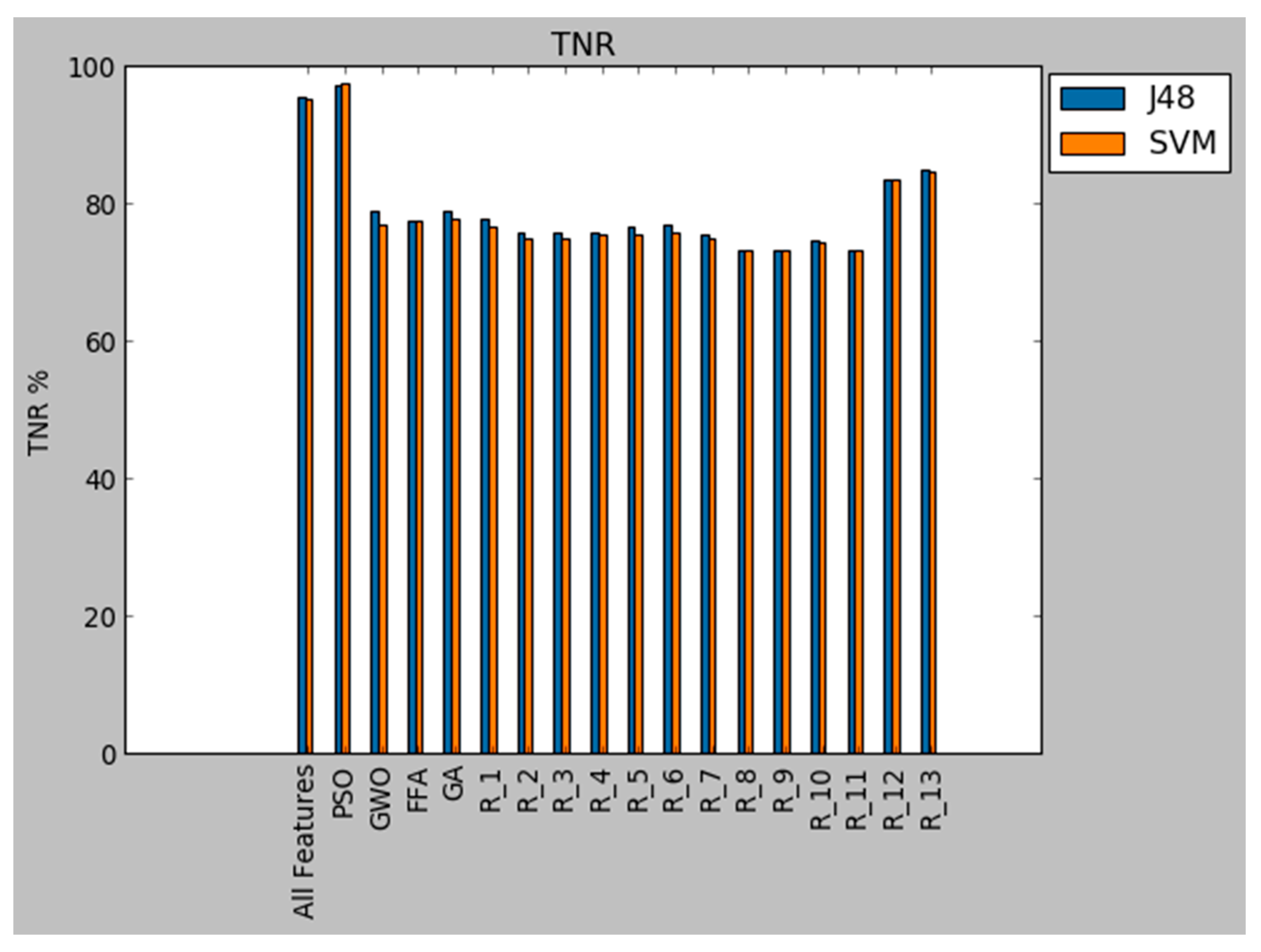
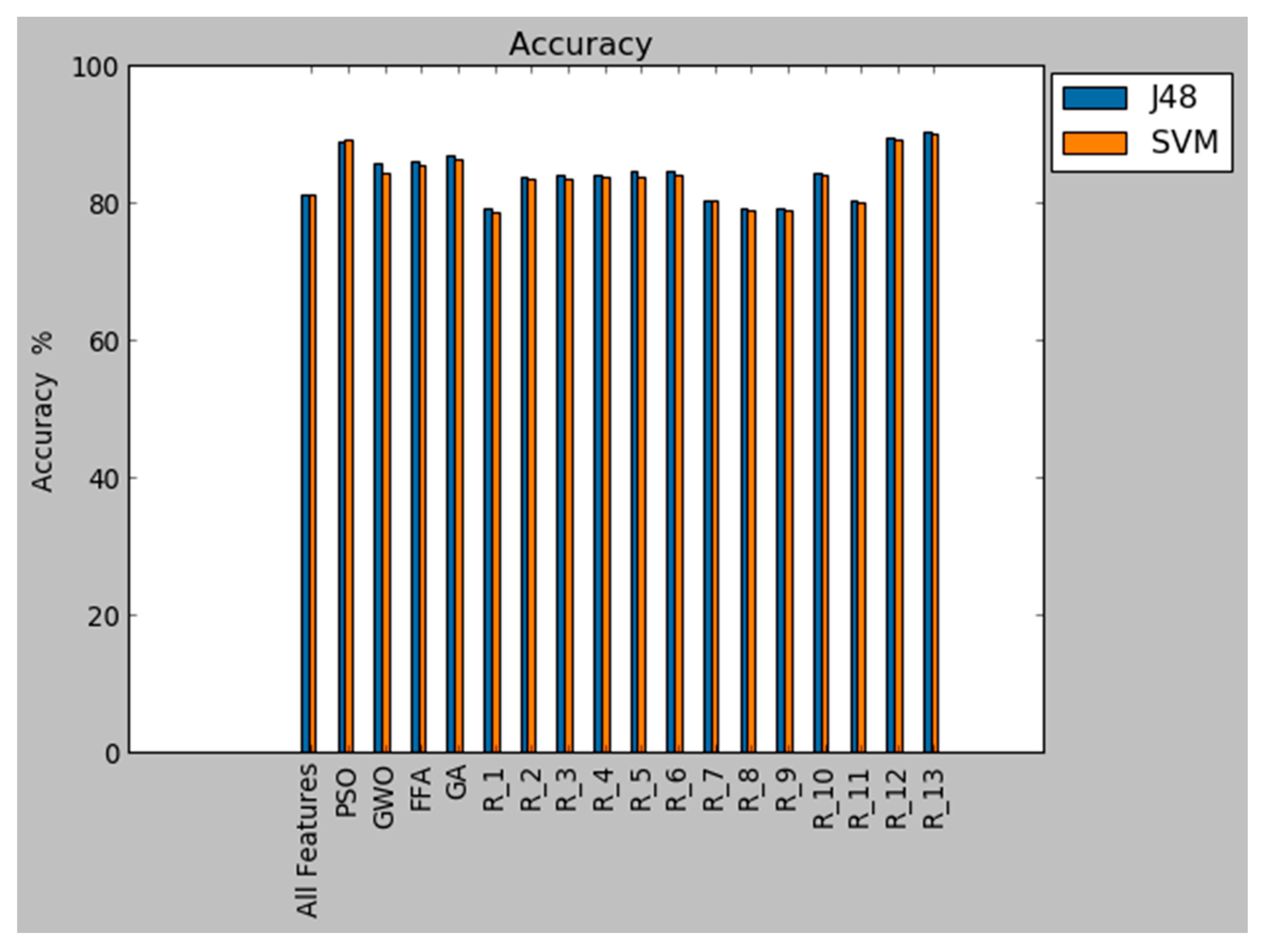
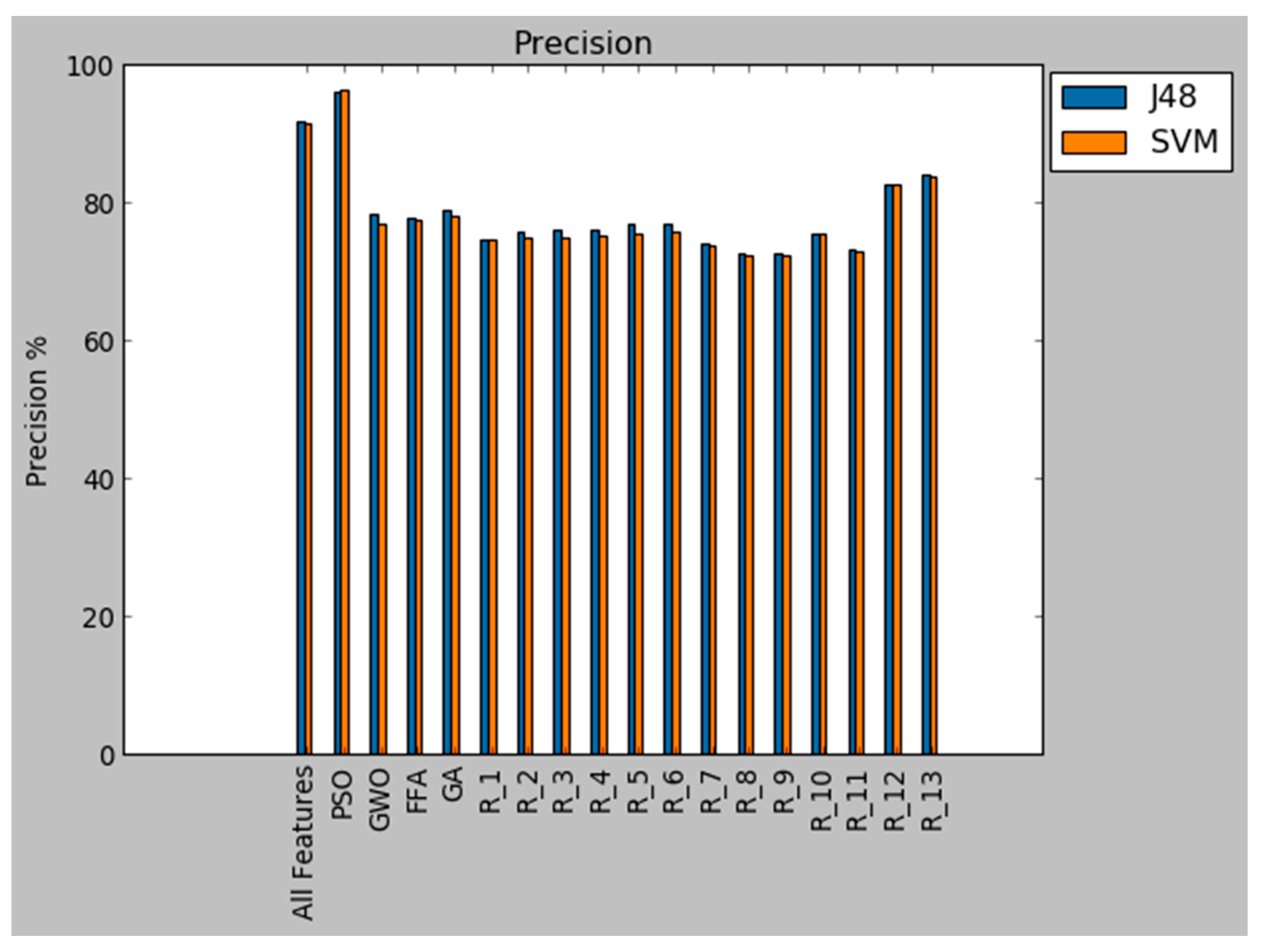
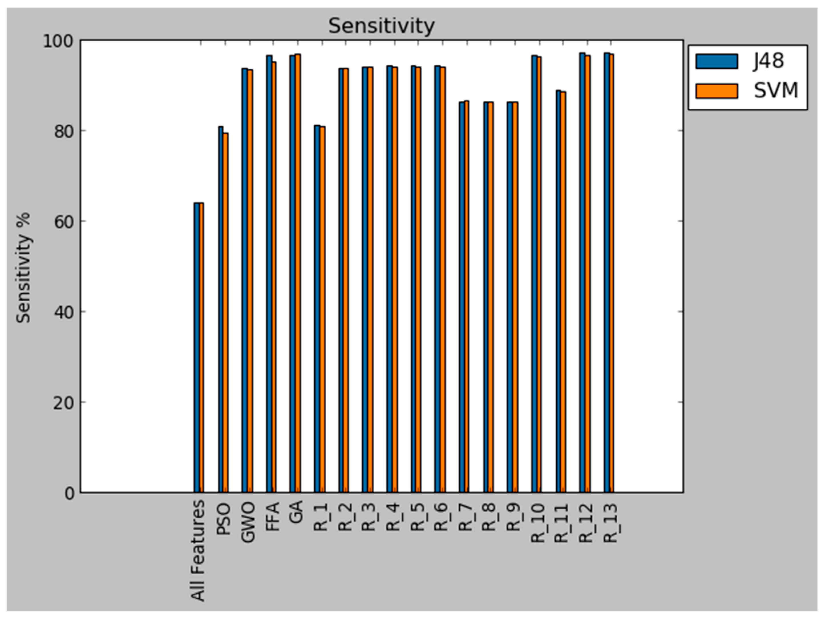
| Rule | TPR | FNR | FPR | TNR | Accuracy | Precision | Sensitivity | F-Measure |
|---|---|---|---|---|---|---|---|---|
| All | 63.99% | 36.01% | 4.57% | 95.42% | 81.29% | 91.94% | 63.98% | 75.46% |
| PSO | 80.844% | 19.156% | 2.817% | 97.183% | 89.013% | 96.107% | 80.844% | 87.817% |
| GWO | 93.797% | 6.203% | 20.952% | 79.048% | 85.676% | 78.513% | 93.797% | 85.477% |
| FFA | 96.586% | 3.414% | 22.592% | 77.408% | 86.037% | 77.764% | 96.586% | 86.159% |
| GA | 96.700% | 3.300% | 21.164% | 78.836% | 86.874% | 78.892% | 96.700% | 86.893% |
| R1 | 81.097% | 18.903% | 22.331% | 77.669% | 79.210% | 74.774% | 81.097% | 77.807% |
| R2 | 93.854% | 6.146% | 24.307% | 75.693% | 83.854% | 75.912% | 93.854% | 83.935% |
| R3 | 94.124% | 5.876% | 24.307% | 75.693% | 83.976% | 75.965% | 94.124% | 84.075% |
| R4 | 94.314% | 5.686% | 24.307% | 75.693% | 84.061% | 76.001% | 94.314% | 84.173% |
| R5 | 94.314% | 5.686% | 23.204% | 76.796% | 84.668% | 76.838% | 94.314% | 84.684% |
| R6 | 94.314% | 5.686% | 22.984% | 77.016% | 84.790% | 77.008% | 94.314% | 84.786% |
| R7 | 86.481% | 13.519% | 24.537% | 75.463% | 80.415% | 74.205% | 86.481% | 79.874% |
| R8 | 86.349% | 13.651% | 26.681% | 73.319% | 79.175% | 72.539% | 86.349% | 78.844% |
| R9 | 86.349% | 13.651% | 26.681% | 73.319% | 79.175% | 72.539% | 86.349% | 78.844% |
| R10 | 96.549% | 3.451% | 25.410% | 74.590% | 84.458% | 75.617% | 96.549% | 84.810% |
| R11 | 89.051% | 10.949% | 26.681% | 73.319% | 80.389% | 73.148% | 89.051% | 80.320% |
| R12 | 97.127% | 2.873% | 16.587% | 83.413% | 89.576% | 82.697% | 97.127% | 89.333% |
| R13 | 97.141% | 2.859% | 14.950% | 85.050% | 90.484% | 84.136% | 97.141% | 90.172% |
| Rules | TPR | FNR | FPR | TNR | Accuracy | Precision | Sensitivity | F-Measure |
|---|---|---|---|---|---|---|---|---|
| All | 63.965% | 36.035% | 4.809% | 95.191% | 81.158% | 91.566% | 63.965% | 75.316% |
| PSO | 79.562% | 20.438% | 2.596% | 97.404% | 89.152% | 96.345% | 79.562% | 87.153% |
| GWO | 93.570% | 6.430% | 22.931% | 77.069% | 84.485% | 76.908% | 93.570% | 84.425% |
| FFA | 95.235% | 4.765% | 22.592% | 77.408% | 85.429% | 77.519% | 95.235% | 85.469% |
| GA | 96.970% | 3.030% | 22.270% | 77.730% | 86.387% | 78.079% | 96.970% | 86.505% |
| R1 | 80.827% | 19.173% | 23.265% | 76.735% | 78.576% | 74.774% | 80.827% | 77.248% |
| R2 | 93.884% | 6.116% | 24.994% | 75.006% | 83.388% | 74.998% | 93.884% | 83.385% |
| R3 | 94.154% | 5.846% | 24.994% | 75.006% | 83.508% | 75.052% | 94.154% | 83.525% |
| R4 | 94.154% | 5.846% | 24.562% | 75.438% | 83.748% | 75.377% | 94.154% | 83.726% |
| R5 | 94.154% | 5.846% | 24.346% | 75.654% | 83.868% | 75.540% | 94.154% | 83.826% |
| R6 | 94.154% | 5.846% | 24.130% | 75.870% | 83.988% | 75.705% | 94.154% | 83.927% |
| R7 | 86.751% | 13.249% | 24.978% | 75.022% | 80.293% | 73.923% | 86.751% | 79.825% |
| R8 | 86.403% | 13.597% | 26.902% | 73.098% | 79.077% | 72.387% | 86.403% | 78.776% |
| R9 | 86.403% | 13.597% | 26.902% | 73.098% | 79.077% | 72.387% | 86.403% | 78.776% |
| R10 | 96.278% | 3.722% | 25.631% | 74.369% | 84.215% | 75.405% | 96.278% | 84.573% |
| R11 | 88.781% | 11.219% | 26.902% | 73.098% | 80.146% | 72.926% | 88.781% | 80.077% |
| R12 | 96.586% | 3.414% | 16.587% | 83.413% | 89.333% | 82.617% | 96.586% | 89.058% |
| R13 | 96.870% | 3.130% | 15.391% | 84.609% | 90.119% | 83.706% | 96.870% | 89.808% |
© 2020 by the author. Licensee MDPI, Basel, Switzerland. This article is an open access article distributed under the terms and conditions of the Creative Commons Attribution (CC BY) license (http://creativecommons.org/licenses/by/4.0/).
Share and Cite
Almomani, O. A Feature Selection Model for Network Intrusion Detection System Based on PSO, GWO, FFA and GA Algorithms. Symmetry 2020, 12, 1046. https://doi.org/10.3390/sym12061046
Almomani O. A Feature Selection Model for Network Intrusion Detection System Based on PSO, GWO, FFA and GA Algorithms. Symmetry. 2020; 12(6):1046. https://doi.org/10.3390/sym12061046
Chicago/Turabian StyleAlmomani, Omar. 2020. "A Feature Selection Model for Network Intrusion Detection System Based on PSO, GWO, FFA and GA Algorithms" Symmetry 12, no. 6: 1046. https://doi.org/10.3390/sym12061046