Article

Multiquadrics without the Shape Parameter for Solving Partial Differential Equations

School of Engineering, Department of Harbor and River Engineering, National Taiwan Ocean University, Keelung 20224, Taiwan
*
Authors to whom correspondence should be addressed.
Symmetry 2020, 12(11), 1813; https://doi.org/10.3390/sym12111813
Submission received: 10 October 2020 / Revised: 30 October 2020 / Accepted: 30 October 2020 / Published: 2 November 2020

Abstract

:
In this article, we present multiquadric radial basis functions (RBFs), including multiquadric (MQ) and inverse multiquadric (IMQ) functions, without the shape parameter for solving partial differential equations using the fictitious source collocation scheme. Different from the conventional collocation method that assigns the RBF at each center point coinciding with an interior point, we separated the center points from the interior points, in which the center points were regarded as the fictitious sources collocated outside the domain. The interior, boundary, and source points were therefore collocated within, on, and outside the domain, respectively. Since the radial distance between the interior point and the source point was always greater than zero, the MQ and IMQ RBFs and their derivatives in the governing equation were smooth and globally infinitely differentiable. Accordingly, the shape parameter was no longer required in the MQ and IMQ RBFs. Numerical examples with the domain in symmetry and asymmetry are presented to verify the accuracy and robustness of the proposed method. The results demonstrated that the proposed method using MQ RBFs without the shape parameter acquires more accurate results than the conventional RBF collocation method with the optimum shape parameter. Additionally, it was found that the locations of the fictitious sources were not sensitive to the accuracy.

1. Introduction

The meshfree methods recognized as powerful tools to solve practical problems governed by partial differential equations (PDEs) have attracted considerable attention [1,2,3]. These methods have the advantage that it does not require mesh construction [4]. Engineering problems involving irregular geometry are usually intractable. For such problems, the use of the meshfree methods to acquire approximate solutions is advantageous. Several meshfree methods utilizing approximation functions, such as moving least squares, reproducing kernel collocation method, Trefftz method, and element-free Galerkin method [5,6], have been widely used for solving engineering problems. The complexities involved in the solution of the governing equations require advanced mathematical approaches, such as the radial basis function collocation method (RBFCM) [7,8]. The development of the RBFCM in the application of advanced mathematical modeling has raised much attention recently because of its meshfree characteristics and computational efficiency [9,10]. The RBFCM is probably one of the popular methods for finding the solutions of boundary value problems with the domain in symmetry and asymmetry where the variables could be expressed by using the function approximation [11,12].
A variety of the radial basis functions (RBFs) may be adopted, such as the Gaussian [13], multiquadric (MQ) [14], inverse multiquadric (IMQ) [15], and thin plate spline (TPS) functions [16]. Among them, the multiquadric function may obtain more accurate solutions than other RBF interpolations [8] and is often utilized as the RBF interpolation for dealing with PDEs. In the MQ interpolation, the role of an arbitrary constant, namely, the shape parameter, is necessary. Attempts to identify the optimum shape parameter have been widely investigated [17,18,19,20]; however, identifying the suitable shape parameter in the MQ interpolation remains an issue.
Numerical examples, including a two-dimensional wave problem, a two-dimensional groundwater flow problem, and a two-dimensional unsaturated flow problem, are presented to verify the accuracy and robustness of the proposed method. This article is arranged as follows. In Section 2, we present the formulation of the proposed collocation method. Section 3 is devoted to accuracy and convergence analysis. In Section 4, numerical examples are presented. Finally, the main findings of this article are summarized in Section 5.

2. The Collocation Method of the Multiquadric Radial Basis Function

The boundary value problem in two dimensions is:
Δ u ( x ) + D u ( x ) x + E u ( x ) y + G u ( x ) = H in Ω
u ( x ) = b ( x )   on   Ω ,
where Δ is the Laplace operator, u ( x ) denotes the unknown, x = ( x , y ) , Ω is a bounded domain with boundary Ω , b ( x ) represents the function boundary values, and D, E, G, and H are given constants. Using the RBFCM, we may write the unknown by the radial basis function as follows:
u ( x ) = j = 1 M λ j φ ( r j )
where r j is the radial distance, r j = | x s j | , φ ( r j ) is the basis function, x is a point inside the domain, s j is the center point, M is the total number of center points, and λ j is the unknown coefficient to be determined.
In the RBFCM, the RBFs, such as MQ and IMQ, are defined by a constant called the shape parameter. The MQ interpolation method was first developed by Hardy, after which Franke [21] depicted that the MQ interpolation may be one of the best methods among many interpolation schemes based on accuracy, stability, and efficiency. The RBFCM with MQ is also named the Kansa method [2]. The MQ RBF is expressed.
φ M Q ( r j ) = r j 2 + c 2
where c is the shape parameter. The IMQ RBF is expressed as follows:
φ I M Q ( r j ) = 1 r j 2 + c 2
Because of the shape parameter, the MQ and IMQ RBFs and their derivatives become smooth and non-singular functions. Accordingly, the resulting interpolation matrix is also non-singular. Selecting an RBF such that the interpolation matrix is non-singular is exactly a definition for the RBF. Functions, including the Gaussian, inverse quadratic, and IMQ functions, which are completely monotone, have this property. Finding the derivative of the MQ interpolation, we obtain:
j = 1 M λ j r j 2 + 2 c 2 ( r j 2 + c 2 ) 1.5 + j = 1 M λ j D ( x x j ) + E ( y y j ) ( r j 2 + c 2 ) 0.5 + G j = 1 M λ j ( r j 2 + c 2 ) 0.5 = H
Since the MQ RBF is not a solution of the governing Equation (1), the interior points must be collocated inside the domain. The MQ RBF is applied at the center point, which is usually selected to coincide with the interior point, as depicted in Figure 1. From the above equation, we may find that it may be singular when c = 0 at r j = 0 , where the center points coincide with the interior points. The shape parameter, thus, should not be equal to zero to prevent singularity.
A simple collocation algorithm separating the center points from the interior points, in which the center points are regarded as the source points placed outside the domain, is proposed. Different from the conventional RBFCM that utilizes the MQ interpolation at each center point coinciding with an interior point, the center points are regarded as fictitious sources that collocate outside the domain.
The interior, boundary, and source points are therefore collocated within, on, and outside the domain, respectively, as shown in Figure 2. Since the radial distance between the interior point and the source point is always greater than zero, the MQ RBF and its derivatives in the governing equation remain smooth and globally infinitely differentiable.
Accordingly, we eliminate the shape factor from the MQ RBF. Let c = 0 ; the MQ RBF becomes a simple form, φ ( r j ) = r j , which is completely monotone and smooth because r j 0 . Taking c = 0 , we obtain the following equation from (6):
j = 1 M λ j 1 r j + j = 1 M λ j D ( x x j ) + E ( y y j ) r j + G j = 1 M λ j r j = H
Now, we insert (5) into (1). Finding the derivative of (5), we obtain:
j = 1 M λ j r j 2 2 c 2 ( r j 2 + c 2 ) 2.5 j = 1 M λ j D ( x x j ) + E ( y y j ) ( r j 2 + c 2 ) 1.5 + G j = 1 M λ j 1 ( r j 2 + c 2 ) 0.5 = H
From the above equation, we obtain φ ( r j ) = 1 r j for c = 0 . Inserting the IMQ RBF into the governing equation, we have:
j = 1 M λ j 1 r j 3 j = 1 M λ j D ( x x j ) + E ( y y j ) r j 3 + G j = 1 M λ j 1 r j = H
The approximate solutions are imposed to satisfy the governing equation with the boundary conditions at the collocation point to evaluate the unknown coefficient. Therefore, we obtain the following system of linear equations:
A α = b ,
where A is an M × N matrix, α refers to the coefficients with a size of N × 1 to be evaluated, b refers to the M × 1 given functions. If M = M i + M b , where M b is the number of boundary points and M i is the number of interior points, then Equation (10) is expressed as:
[ A I A B ] [ α ] = [ b I b B ] ,
where A I is the M i × N matrix from the interior points, A B is the M b × N matrix from the boundary points, b I is the M i × 1 vector, and b B is the M b × 1 vector. MATLAB software was used for all computational work, including solving the above simultaneous equations. The maximum absolute error (MAE) and root mean square error (RMSE) were used to measure the accuracy, which is defined by:
MAE = maximum | u E ( x i ) u N ( x i ) | ,   1 i M m ,
RMSE = i = 1 M m [ u E ( x i ) u N ( x i ) ] 2 M m ,
where x i refers to the scattered points in the computed domain, M m is the number of measuring points, and u E ( x i ) and u N ( x i ) represent the numerical and exact solutions at the ith scattered points, respectively.

3. Accuracy and Convergence Analysis

Convergence analysis was carried out to compare the proposed approach with the RBFCM. A two-dimensional Laplace problem [7] was expressed as:
Δ u ( x ) = 0 .
An amoeba-like object boundary was defined as:
Ω = { ( x , y ) | x = ρ ( θ ) cos θ ,   y = ρ ( θ ) sin θ } ,   ρ ( θ ) = e ( sin θ sin 2 θ ) 2 + e ( cos θ cos 2 θ ) 2 ,   0 θ 2 π .
The Dirichlet data were given on the boundaries utilizing the exact solution as follows:
u ( x , y ) = cos ( x ) cosh ( y ) + sin ( x ) sinh ( y ) .
In this example, there are a total of 88 interior points, 238 source points, and 150 boundary points. The source points were collocated outside the domain based on the following equation:
x j s = η ρ j s ( cos θ j s , sin θ j s ) , j = 1 , , M s ,
where x j s = ( x j s , y j s ) is a source point, η represents the dilation parameter, M s is the number of the source points, θ j s represents the angle of source point, and ρ j s represents the radius of the source point.
Because the locations of the source points may alter the accuracy of results, a sensitivity analysis was carried out to examine the accuracy of the MAE versus the dilation parameter. In the sensitivity analysis, we considered the source point placement at different positions outside the two-dimensional amoeba-like region, as shown in Figure 3. Four irregular boundaries of the exterior source collocation, Ω s , defined by the following parametric equations [22]:
Ω s = { ( x j s , y j s ) | x j s = η ρ j s ( θ j s ) cos θ j s ,   y j s = η ρ j s ( θ j s ) sin θ j s } ,
For cases A, B, C, and D in Figure 3, we considered the irregular boundaries of the exterior source collocation, Ω s , defined by (19)–(22), respectively.
ρ j s ( θ j s ) = cos ( 4 θ j s ) + 2 sin 2 4 θ j s 1 / 3 ,   0 θ j s 2 π ,
ρ ( θ j s ) = e ( sin θ j s sin 2 θ j s ) 2 + e ( cos θ j s cos 2 θ j s ) 2 ,   0 θ j s 2 π ,
ρ ( θ j s ) = 16 + cos 2 ( 15 θ j s ) ,   0 θ j s 2 π ,
ρ ( θ j s ) = 8 + cos 5 ( 7 θ j s ) ,   0 θ j s 2 π .
The MAE of the numerical solutions was adopted to evaluate the accuracy of our method. Figure 4 illustrates the MAE of using the Kansa method with different shape parameters and the proposed method with different dilation parameters. In cases A and B, it was found that the MAE decreases with an increase in the shape and dilation parameters—both cases obtain accurate results. However, in cases C and D, it was found that the MAE decreases with an increase in the shape parameter, but that the MAE of the proposed method remains more accurate than that of the Kansa method for different values of the dilation parameter. Additionally, the values of the dilation parameter in the proposed method for cases C and D are less sensitive to the accuracy. These results demonstrate that we obtain accurate results with the use of an arbitrary value in the range of 0–5 for the dilation parameter.
Table 1 presents the results of the MAE and the RMSE for the Kansa method and the proposed approach without the shape parameter. For the Kansa method, the optimum shape parameter was considered. As depicted in Table 1, the RMSE and the MAE adopting the Kansa method are in the order of 10−7 and 10−5, respectively. The RMSE and the MAE, using the proposed approach, are in the order of 10−8 and 10−7, respectively. Our approach acquires more accurate results than the Kansa method, even when the optimum shape parameter is adopted. The proposed method utilizing the exterior source collocation of case D provides a promising solution for the two-dimensional Laplace problem. Results illustrate that the locations of fictitious sources are not sensitive to the accuracy if the fictitious irregular circular boundary is adopted.
The IMQ RBF was further adopted to solve this problem. Figure 5 illustrates the MAE of using the conventional IMQ RBF with different shape parameters and the proposed method with different dilation parameters. Similar to the results obtained in Figure 4, we also obtained accurate solutions with the use of an arbitrary value in the range of 0–5 for the dilation parameter of the proposed IMQ RBF.
Table 2 illustrates the results of the MAE and the RMSE for the conventional IMQ RBF and the proposed method without the shape parameter. The conventional IMQ RBF with the optimum shape parameter was considered. It is clear that the MAE and the RMSE associated with IMQ RBF with the optimum shape parameter are in the order of 10−5 and 10−7, respectively. The MAE and the RMSE, utilizing our method, are in the order of 10−7 and 10−9, respectively. The proposed IMQ RBF adopting the exterior source collocation yields more accurate solutions than the conventional IMQ RBF.

4. Numerical Examples

4.1. A Two-Dimensional Wave Problem

The role of the numerical solutions of the modified Helmholtz equation is essential in the fields of engineering and science, such as in seismic wave propagation problems [23]. The governing equation is:
( Δ λ 2 ) u ( x , y ) = 0 ,
where λ 2 denotes the wave number considered to be 1. In this example, a peanut-like boundary was defined as:
Ω = { ( x , y ) | x = ρ ( θ ) cos θ ,   y = ρ ( θ ) sin θ } ,   ρ ( θ ) = cos 2 θ + 1.1 sin 2 2 θ ,   0 θ 2 π .
The Dirichlet data were given on the boundaries utilizing the following analytical solution:
u ( x , y ) = e ( λ / 2 ) ( x + 3 y ) .
Four approaches considering the conventional RBFCM using MQ and IMQ RBFs and the proposed simple collocation method using MQ and IMQ RBFs without the shape parameter were adopted to solve this wave propagation problem. Figure 6 shows the collocation scheme for the conventional RBFCM, including 135 center points and 150 boundary points. For the proposed collocation method using MQ and IMQ RBFs, as demonstrated in Figure 7, there is a total of 285, 150, and 135 source, boundary, and interior points.
Figure 8 shows a comparison of the MQ RBF for the conventional RBFCM using different shape parameters and the proposed collocation method with different dilation parameters. From Figure 8, the MAE of the conventional RBFCM drastically decreased from 100 to 10−4, while the shape parameter ranged from 0 to 5. The MAE of the proposed collocation method fluctuated between 10−5 and 10−7, while the dilation parameter ranged from 0 to 5.
The IMQ RBF was studied using the same perspective. Based on Figure 9, we confirm that the proposed collocation method using the IMQ RBF without the shape parameter acquires more accurate solutions than the conventional RBFCM.

4.2. A Two-Dimensional Groundwater Flow Problem

Groundwater flow problems often exhibit recharge and leakage from adjacent aquifers that are governed by the Poisson equation [24]. The governing equation of the two-dimensional Poisson equation is:
Δ u ( x , y ) = N .
where N denotes the source term. In this example, the source term is considered to be N = D p 2 [ x cos ( D p y ) + y sin ( D p x ) ] , the coefficient D p is considered to be D p = 0.5 and D p = 10.
The two-dimensional flower-like object boundary was defined as:
Ω = { ( x , y ) | x = ρ ( θ ) cos θ ,   y = ρ ( θ ) sin θ } ,   ρ ( θ ) = cos ( 5 θ ) + 2 sin 2 4 θ 1 / 3 ,   0 θ 2 π .
The Dirichlet data were given on the boundaries utilizing the following analytical solution:
u ( x , y ) = y sin ( π x ) + x cos ( π y ) .
Four approaches considering the conventional RBFCM using MQ and IMQ RBFs and the proposed simple collocation method using MQ and IMQ RBFs without the shape parameter were adopted to solve this groundwater flow problem. Figure 10 shows the collocation scheme for the conventional MQ and IMQ RBFs, containing 99 center points and 150 boundary points. For the proposed collocation method using MQ and IMQ RBFs, as demonstrated in Figure 11, there is a total of 249 source points, 150 boundary points, and 99 interior points. Figure 12 shows a comparison between the MQ RBF for the conventional RBFCM using different shape parameters and the proposed collocation method with different dilation parameters. From Figure 12, the MAE of the conventional RBFCM drastically decreased from 10−1 to 10−4, while the shape parameter ranged from 0 to 5. However, the MAE of our approach remained 10−6, while the dilation parameter ranged from 0 to 5.
The IMQ RBF was studied using the same perspective. Based on Figure 13, we confirm that the proposed collocation method using the IMQ RBF without the shape parameter acquires more accurate solutions than the conventional RBFCM.

4.3. An Unsaturated Flow Problem

The final example under investigation is a two-dimensional unsaturated flow problem [25]. The governing equation is:
x [ K r ( h ) h ( x , z ) x ] + z [ K r ( h ) ( h ( x , z ) z + 1 ) ] = 0 ,
where h is the pressure head and K r ( h ) is the relative hydraulic conductivity. Considering the Gardner model, the following equation is obtained:
2 h ^ ( x , z ) x 2 + 2 h ^ ( x , z ) z 2 + α g h ^ ( x , z ) z = 0 ,
where α g is from the pore size distribution of soil, h ^ is the unknown, which is written as h ^ = e α g h e α g h d , and h d denotes the pressure head with dry soil conditions. Equation (30) is the linearized Richards equation [25]. In this example, the two–dimensional irregular boundary was given as:
Ω = { ( x , z ) | x = ρ ( θ ) cos θ ,   z = ρ ( θ ) sin θ } ,   ρ ( θ ) = cos ( 2 θ ) + 5 cos 2 6 θ ,   0 θ 2 π .
The Dirichlet boundary data were given:
h ^ ( x , z ) = x e α g z .
In this example, α g = 0.5 and h d = 100 . Four approaches considering the conventional RBFCM using MQ and IMQ RBFs and the proposed simple collocation method using MQ and IMQ RBFs without the shape parameter were adopted to solve this problem. Figure 14 shows the collocation scheme for the conventional MQ and IMQ RBFs, containing 147 center points and 150 boundary points. For the proposed collocation method using MQ and IMQ RBFs, as demonstrated in Figure 15, there is a total of 297, 150, and 147 source, boundary, and interior points.
Figure 16 shows a comparison of the MQ RBF for the conventional RBFCM using different shape parameters and the proposed collocation method with different dilation parameters. In Figure 16, the MAE of the conventional RBFCM decreased with an increase in the shape parameter. The MAE of the proposed method, however, remained more accurate than the conventional MQ RBF for different dilation parameter values.
The IMQ RBF was studied using the same perspective. Based on Figure 17, we confirm that the proposed collocation method using the IMQ RBF without the shape parameter acquires more accurate solutions than the conventional RBFCM.
As shown in Figure 18, the computed heads from the proposed method were compared with those of the conventional RBFCM using MQ RBF and the exact solution. The results using the proposed method are consistent with those of the analytical solution.

5. Conclusions

In this article, we presented RBFs, including MQ and IMQ, without the shape parameter for solving partial differential equations using the fictitious source collocation scheme. The concepts of the proposed approach were clearly described in detail. Our findings are concluded as follows:
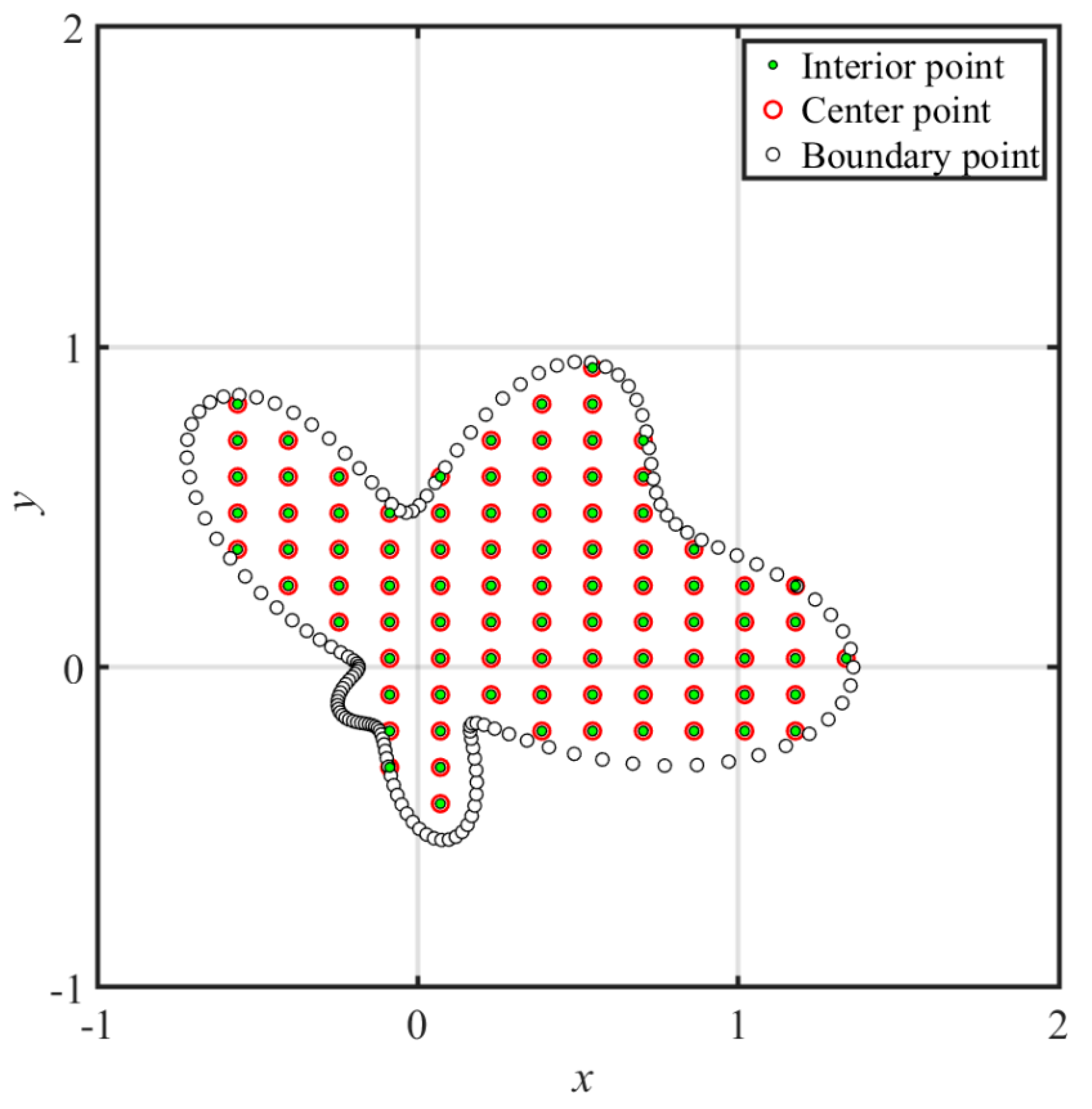
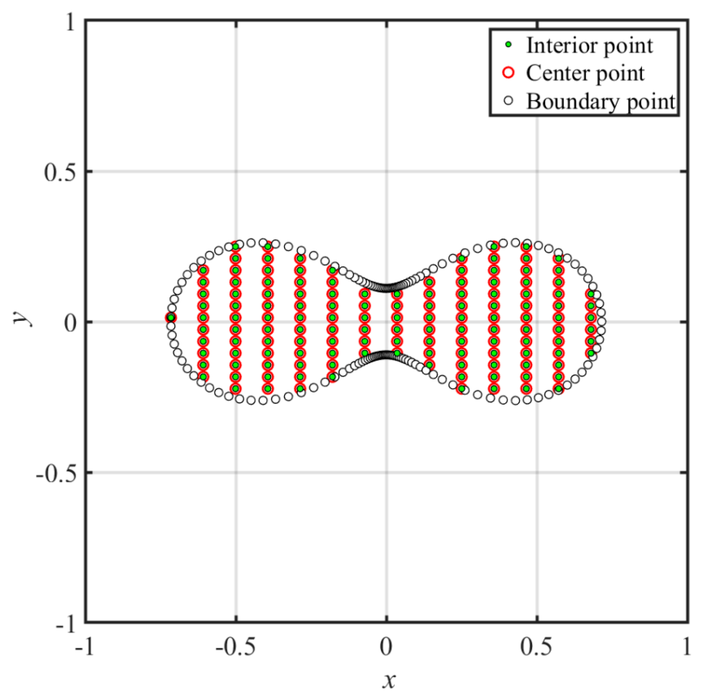
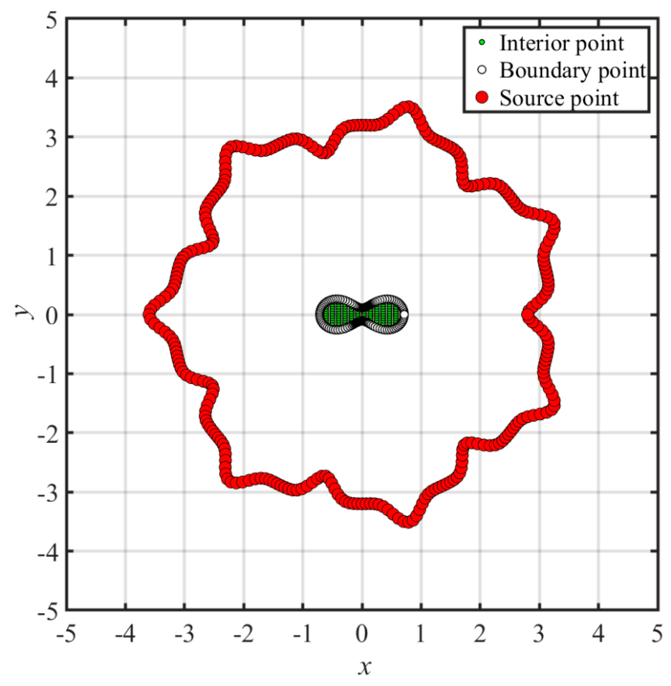
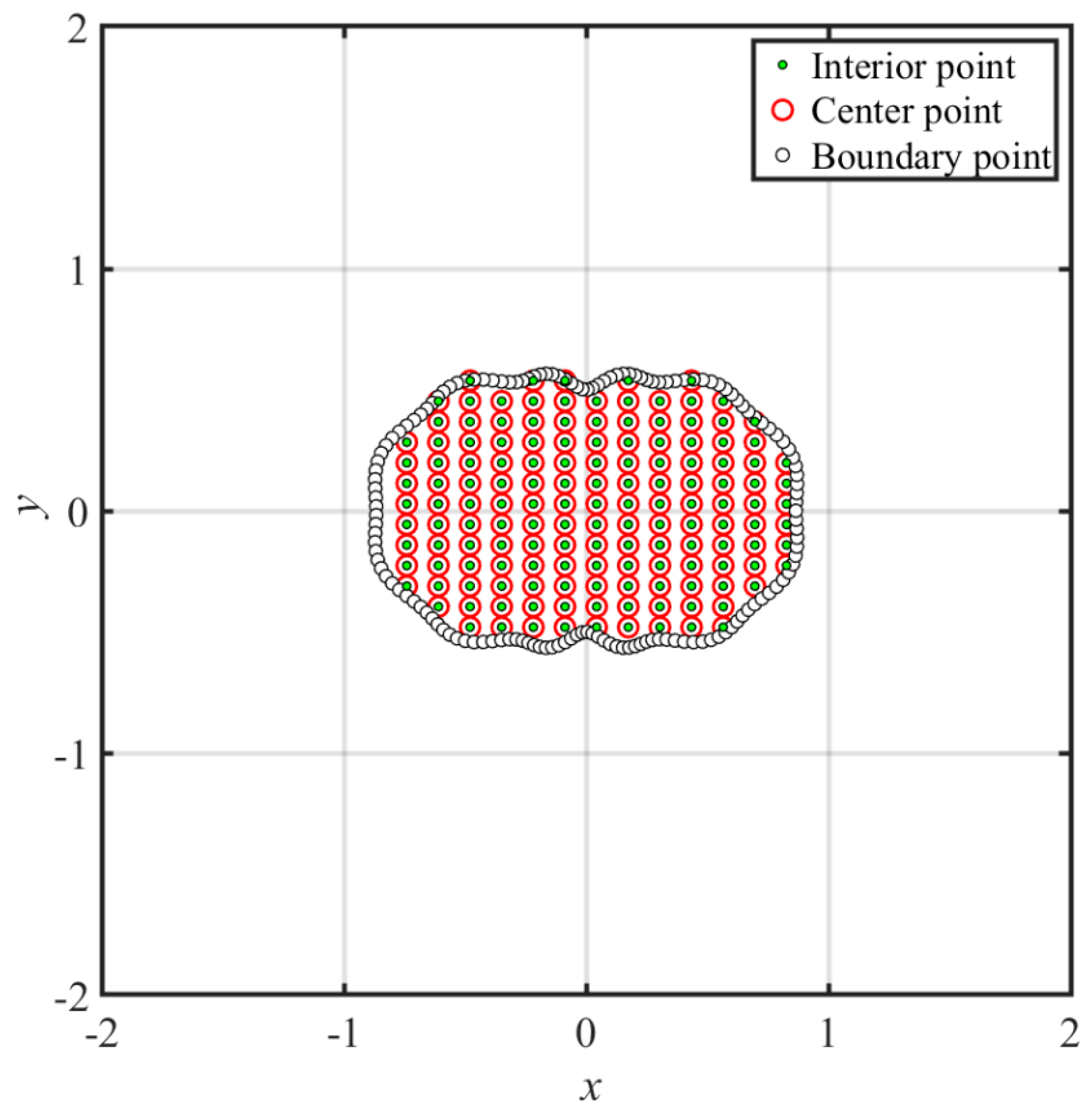
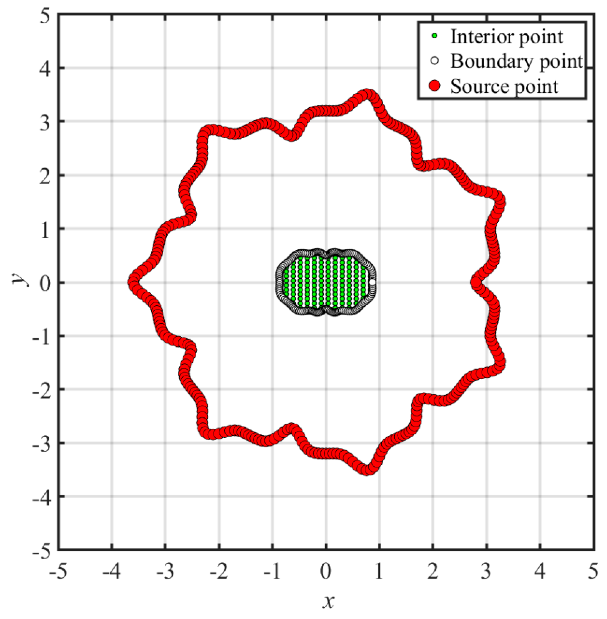
  • We considered the center point as the fictitious source collocated outside the domain. The radial distance between the interior point and the source point was, therefore, always greater than zero. As a result, the MQ and IMQ RBFs and their derivatives in the governing equation were smooth and globally infinitely differentiable. Boundary value problems are solved by the proposed collocation method using MQ and IMQ RBFs without the shape parameter.
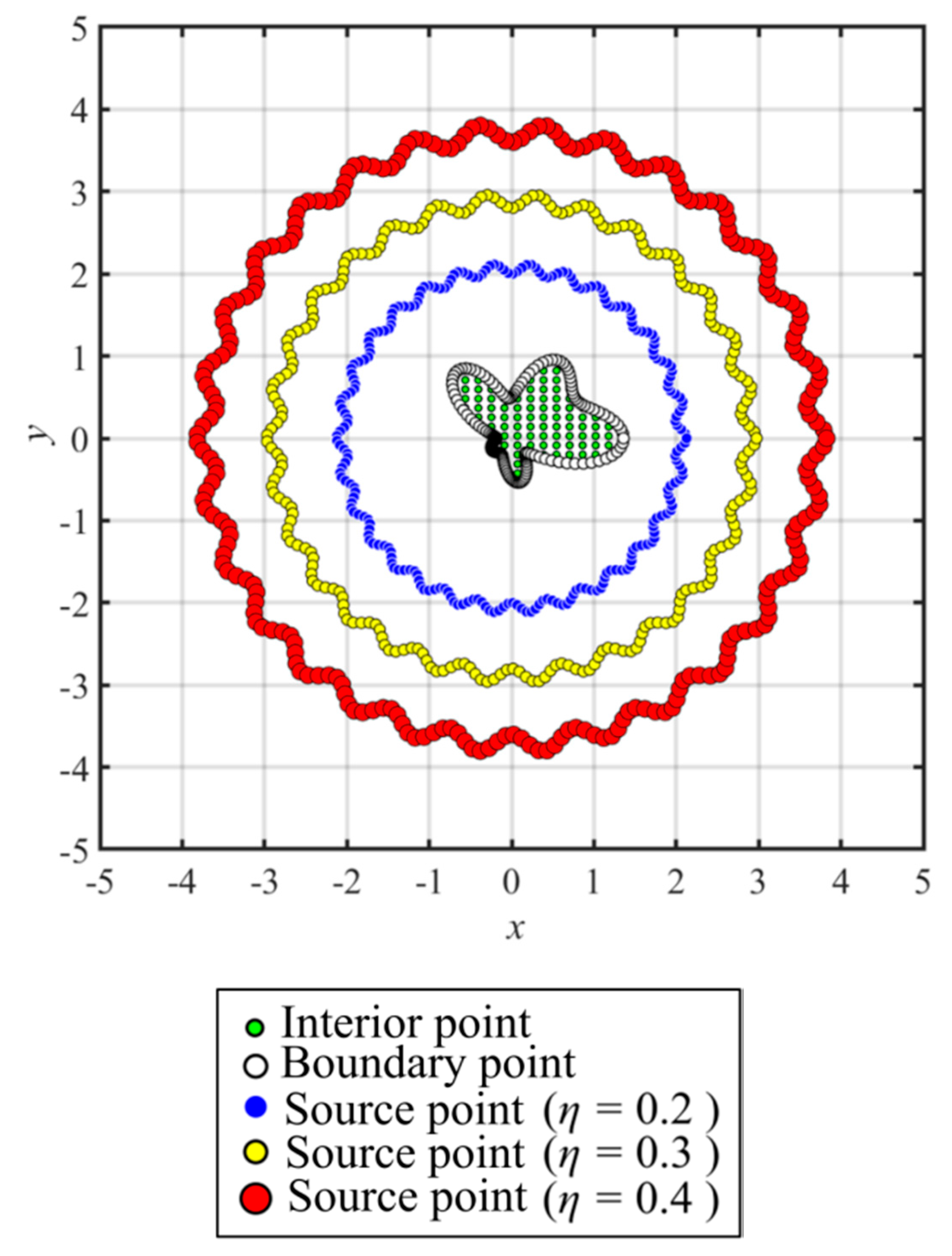
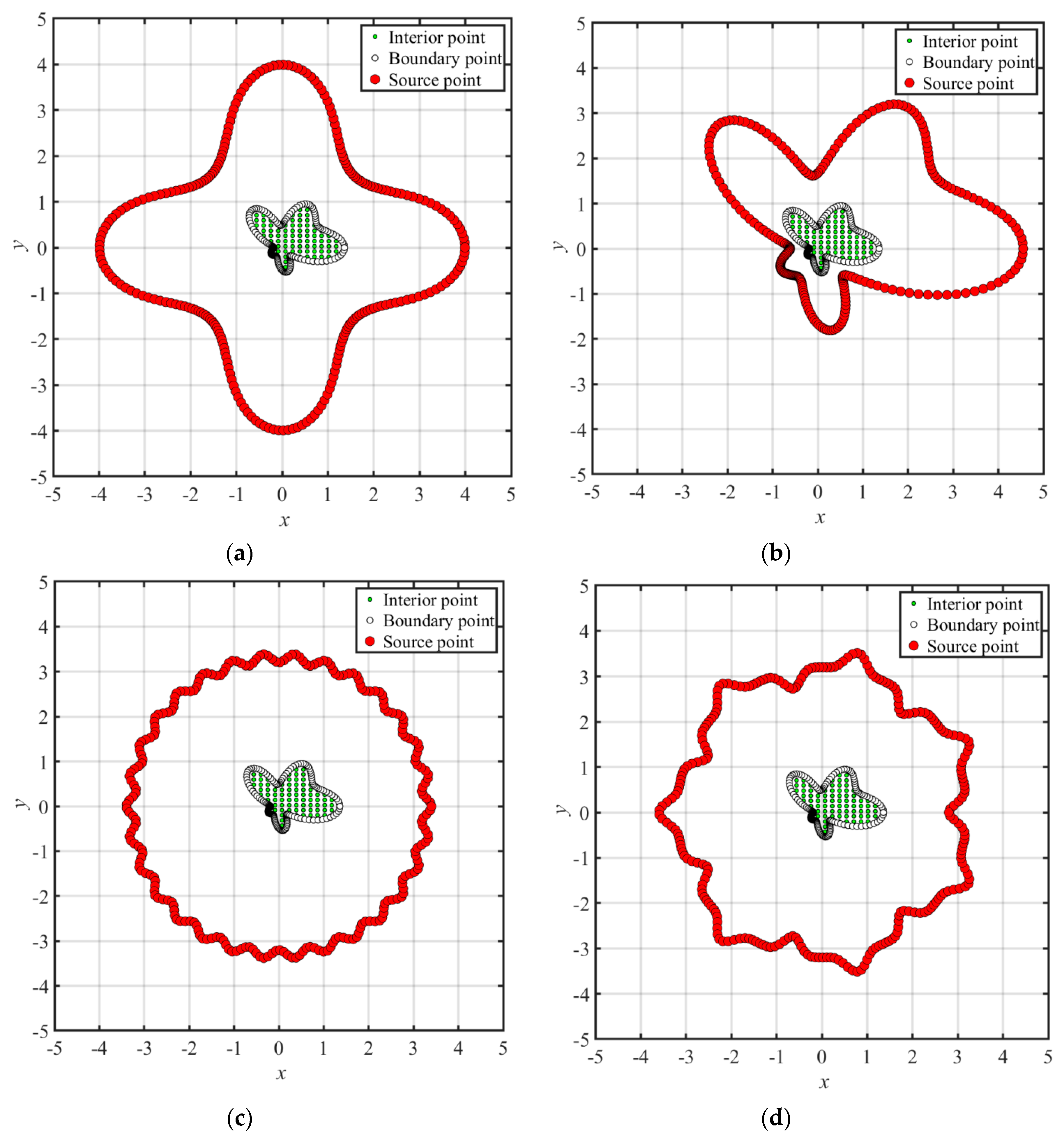
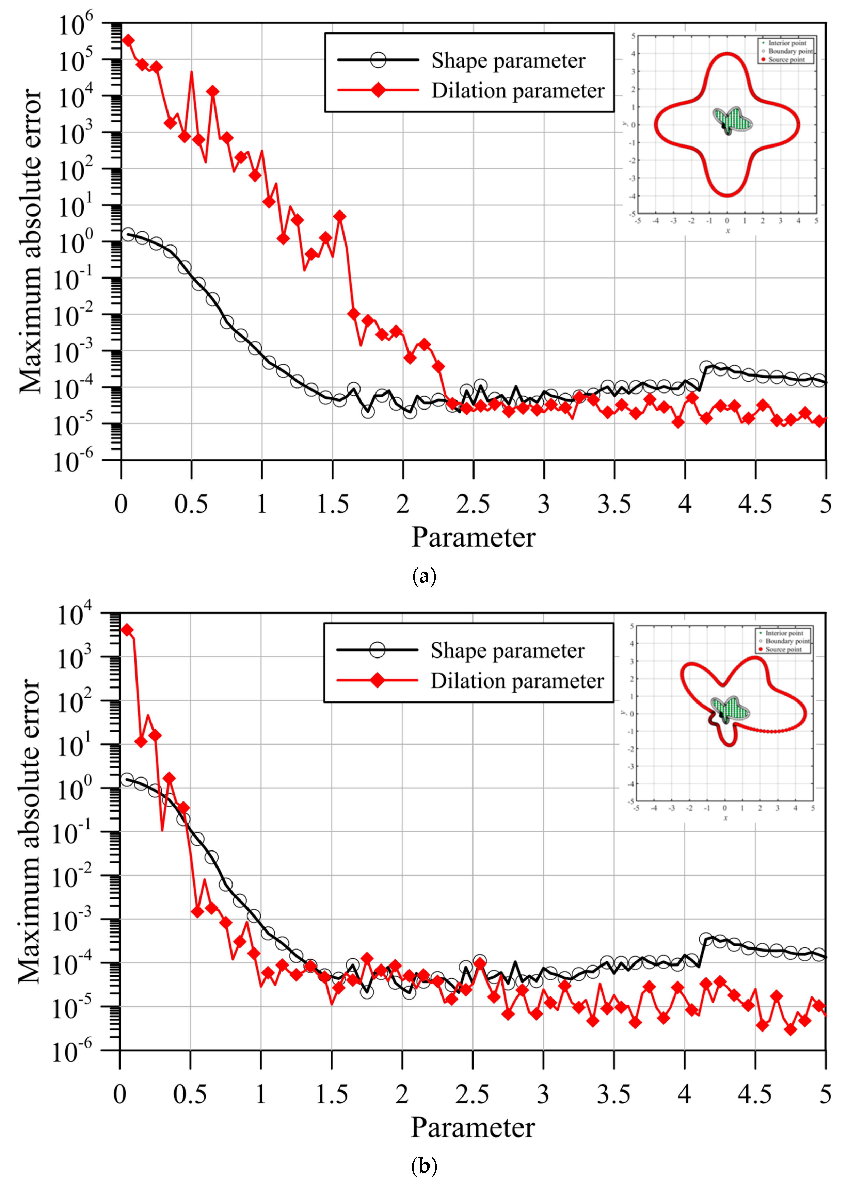
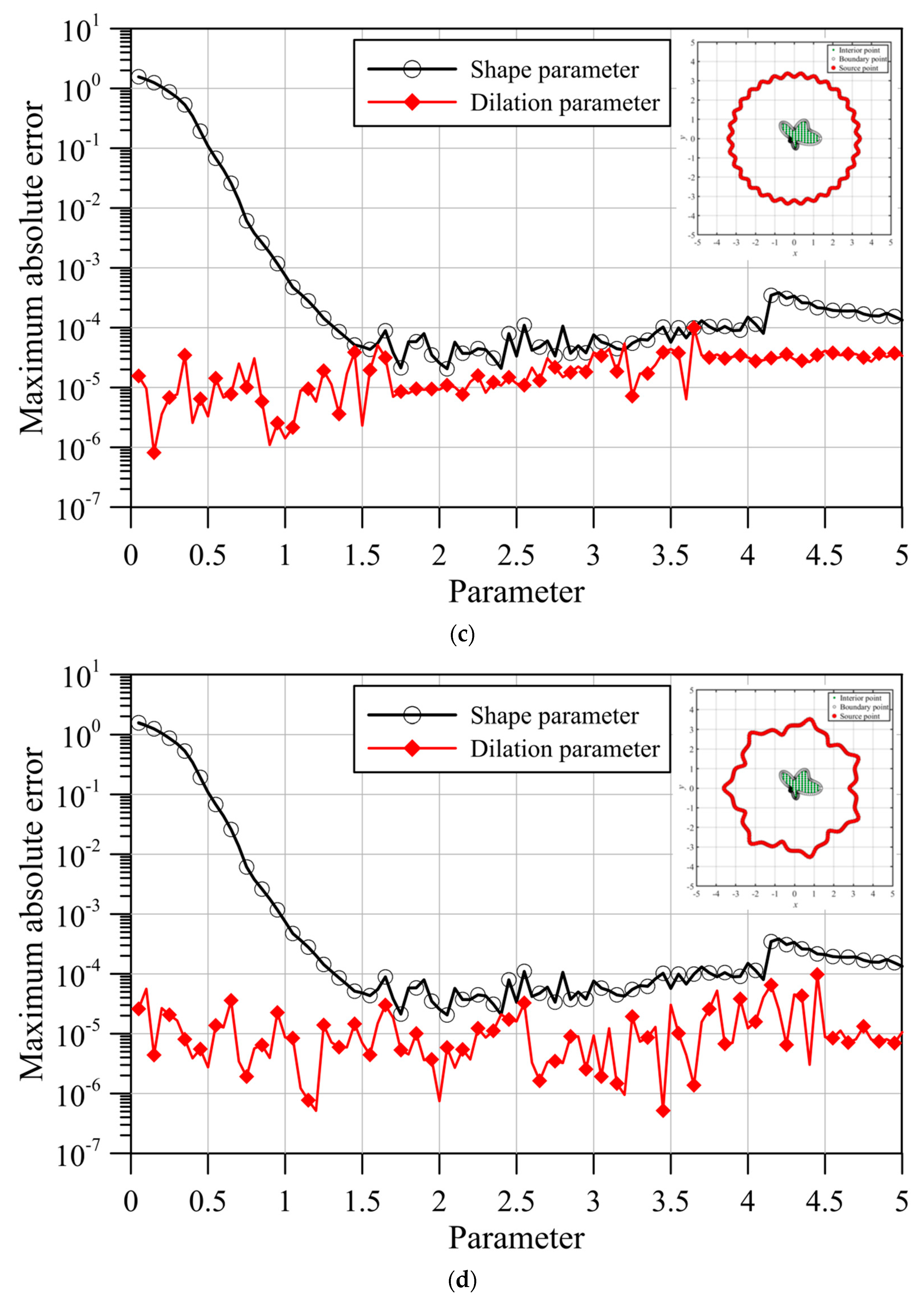
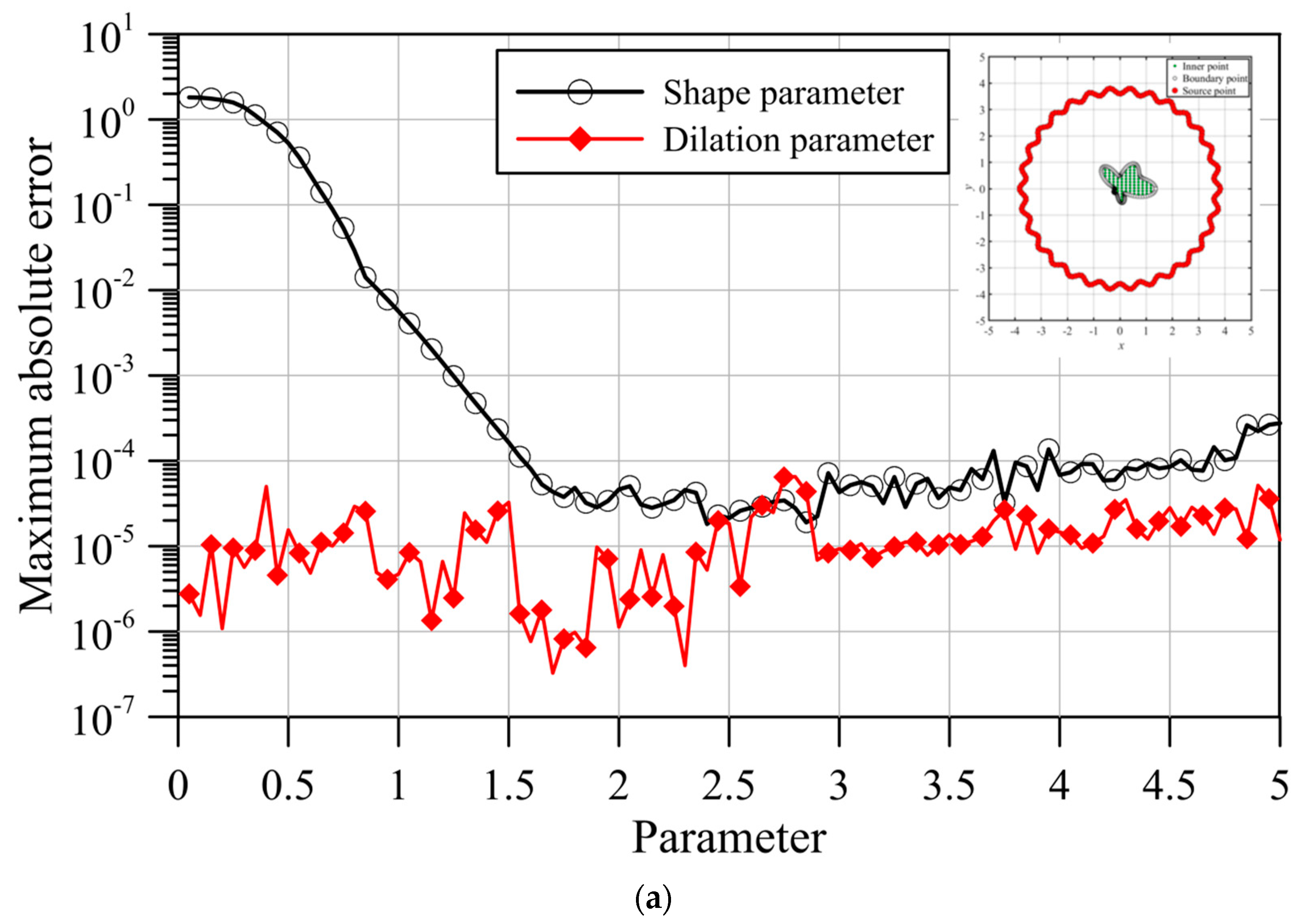
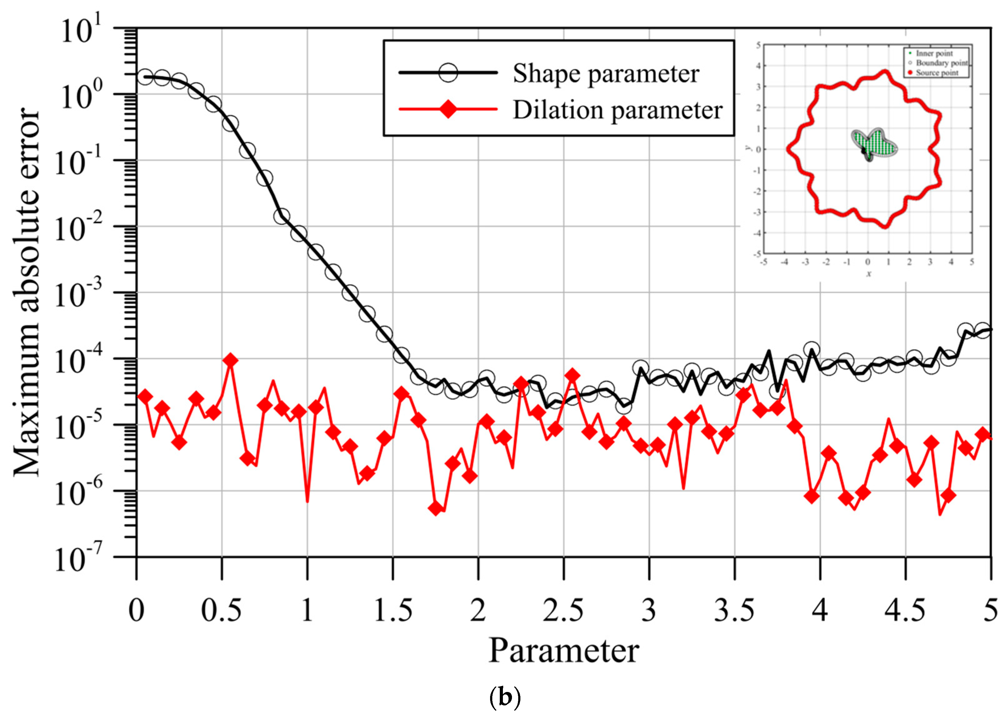
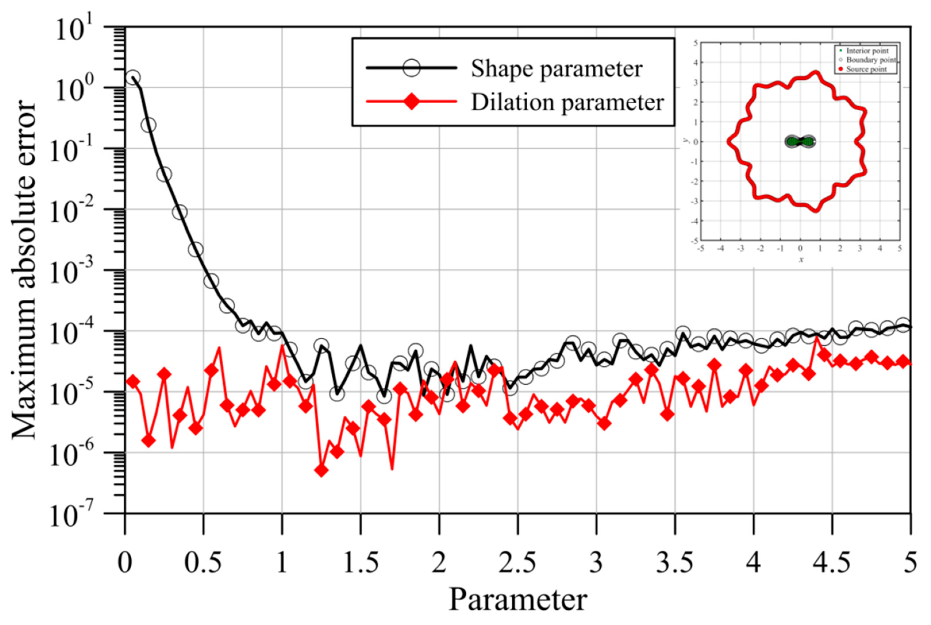
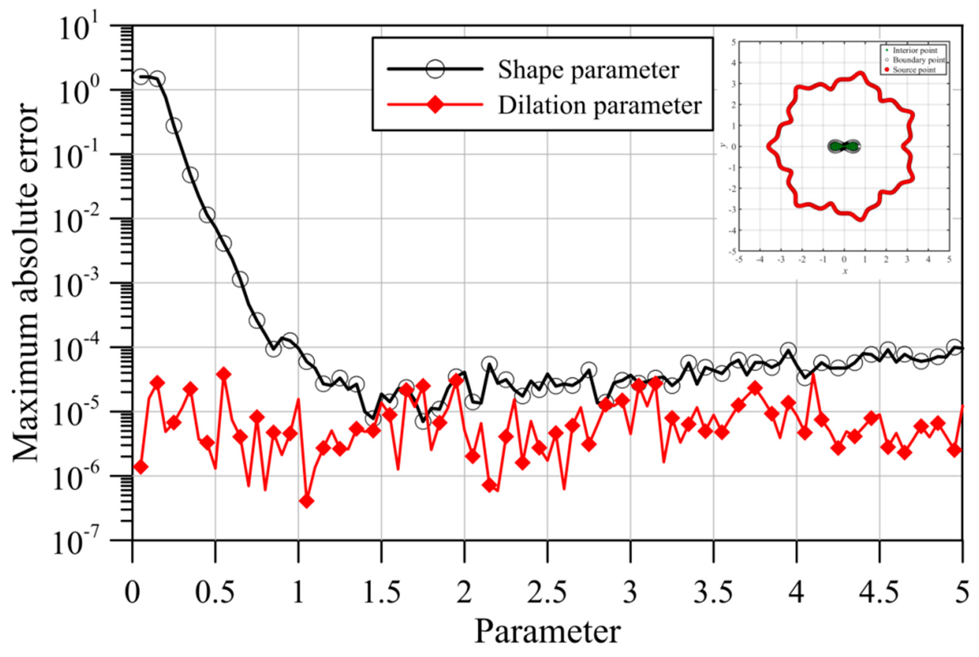
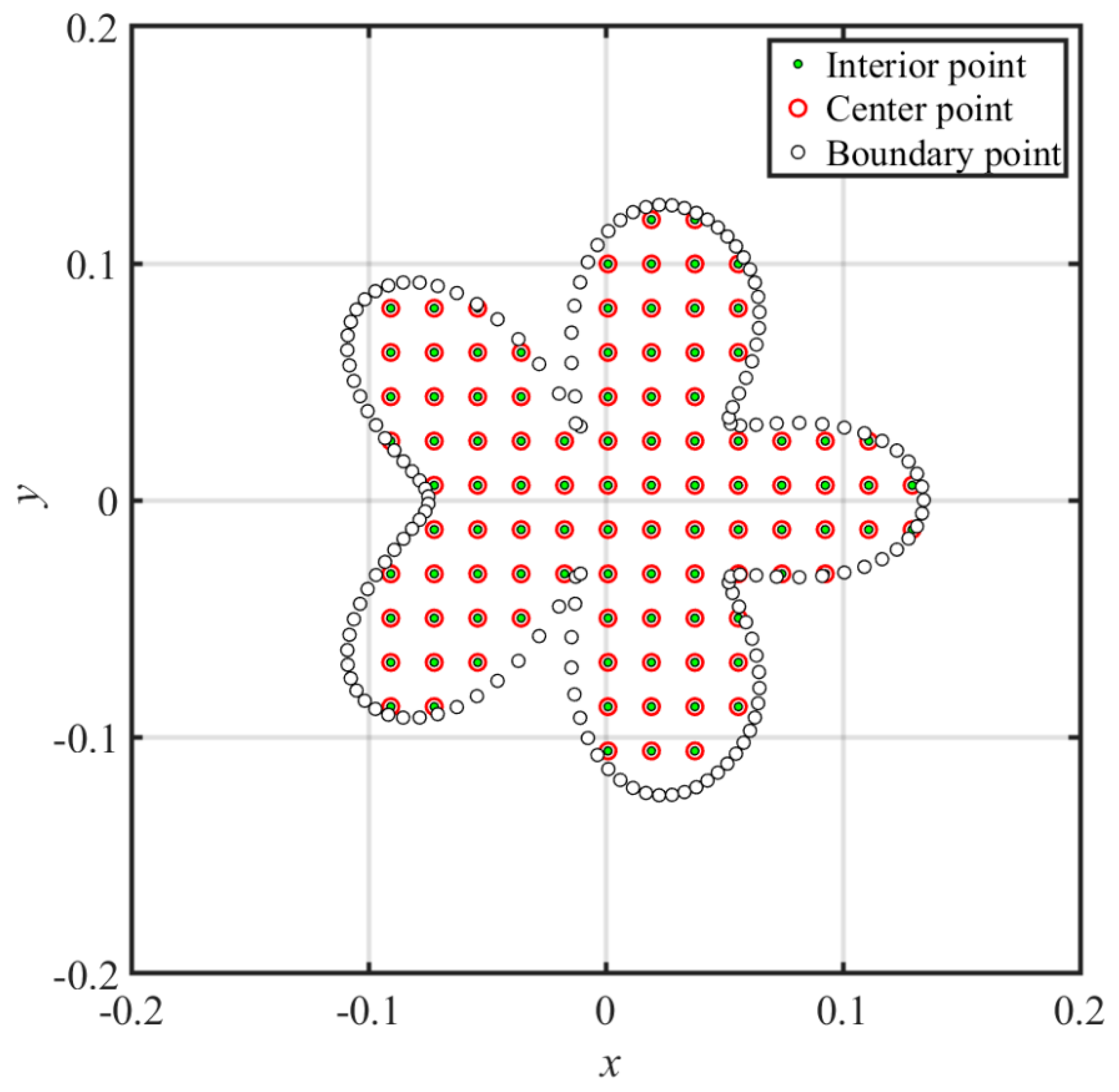
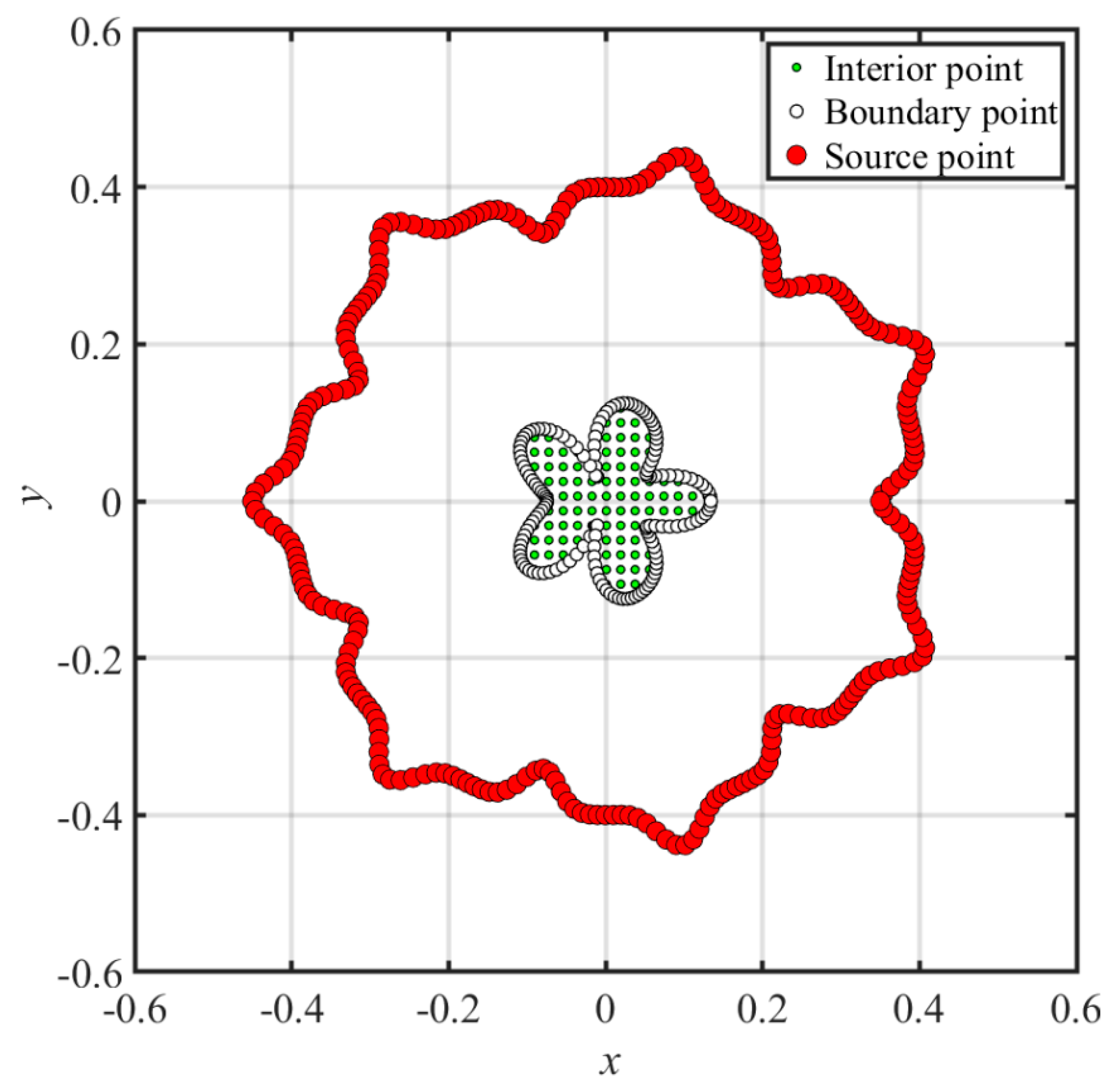
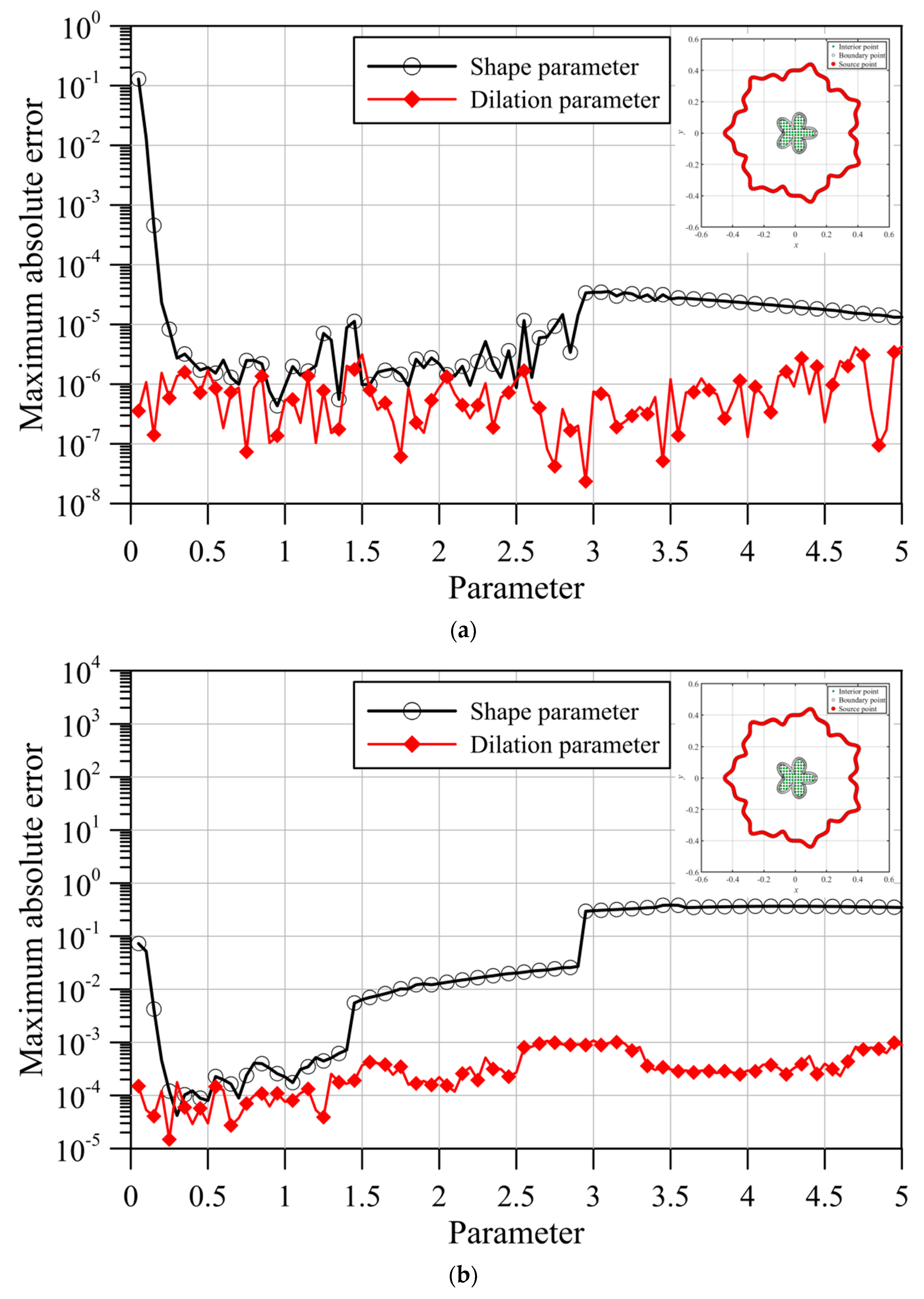
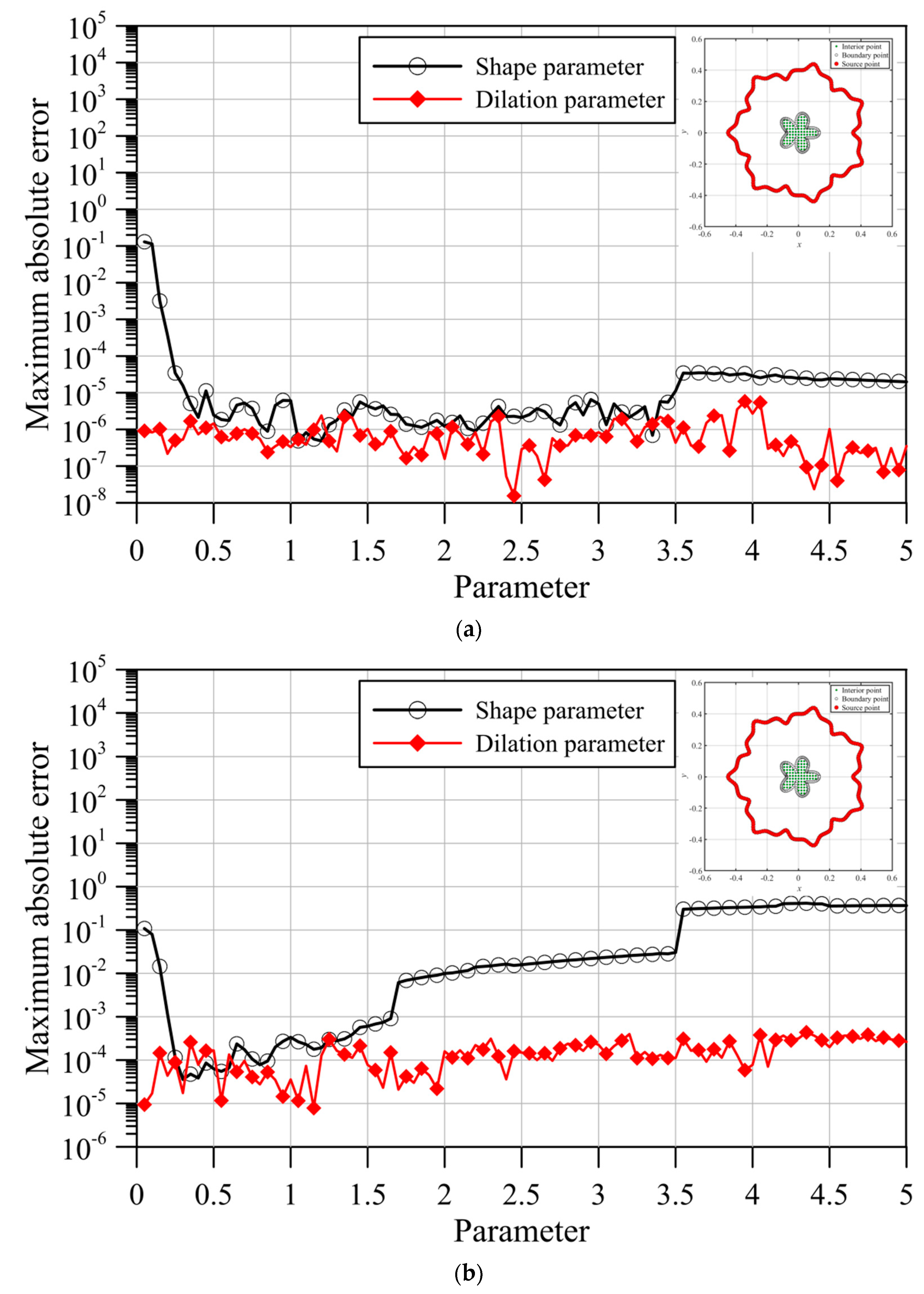
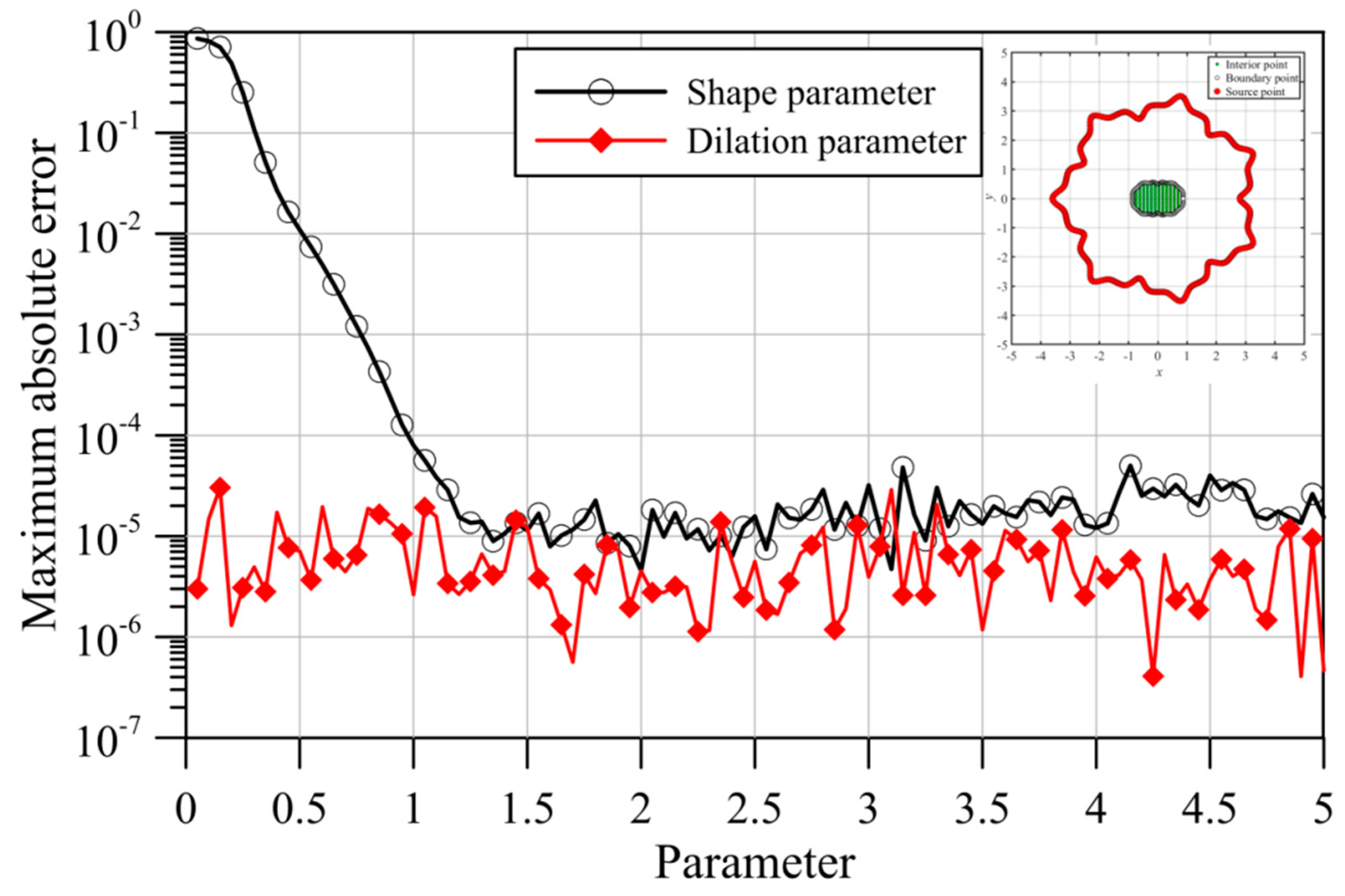
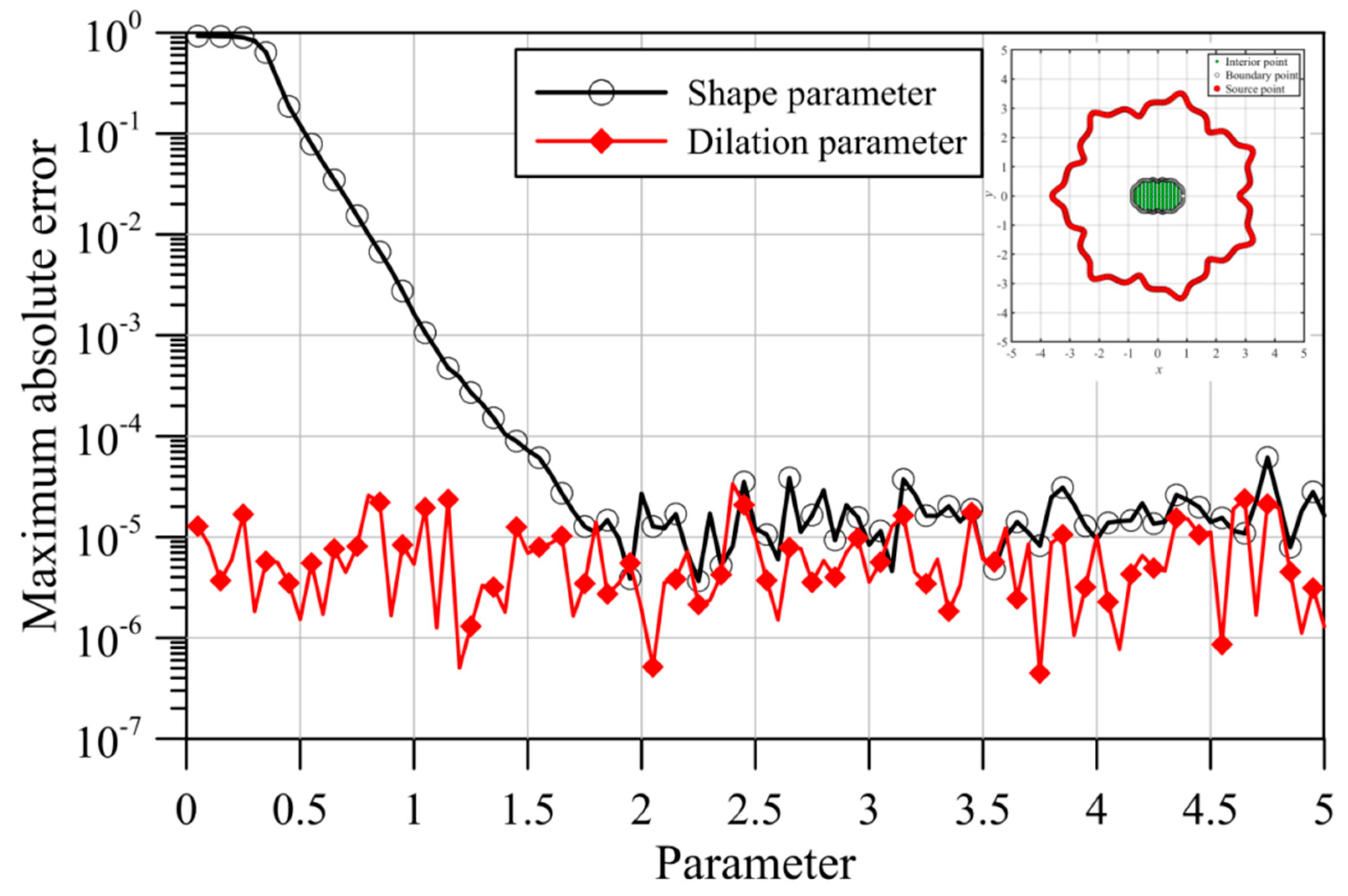
  • The fictitious boundary shape surrounded by the source points and the locations of the source points may affect the accuracy. We conducted a sensitivity analysis to examine the accuracy. In the sensitivity analysis, we investigated the source points placed at different positions outside the domain. Moreover, four irregular fictitious boundary shapes surrounded by the source points were studied. Results illustrate that the locations of fictitious sources are not sensitive to the accuracy if the suggested fictitious irregular circular boundary is adopted.
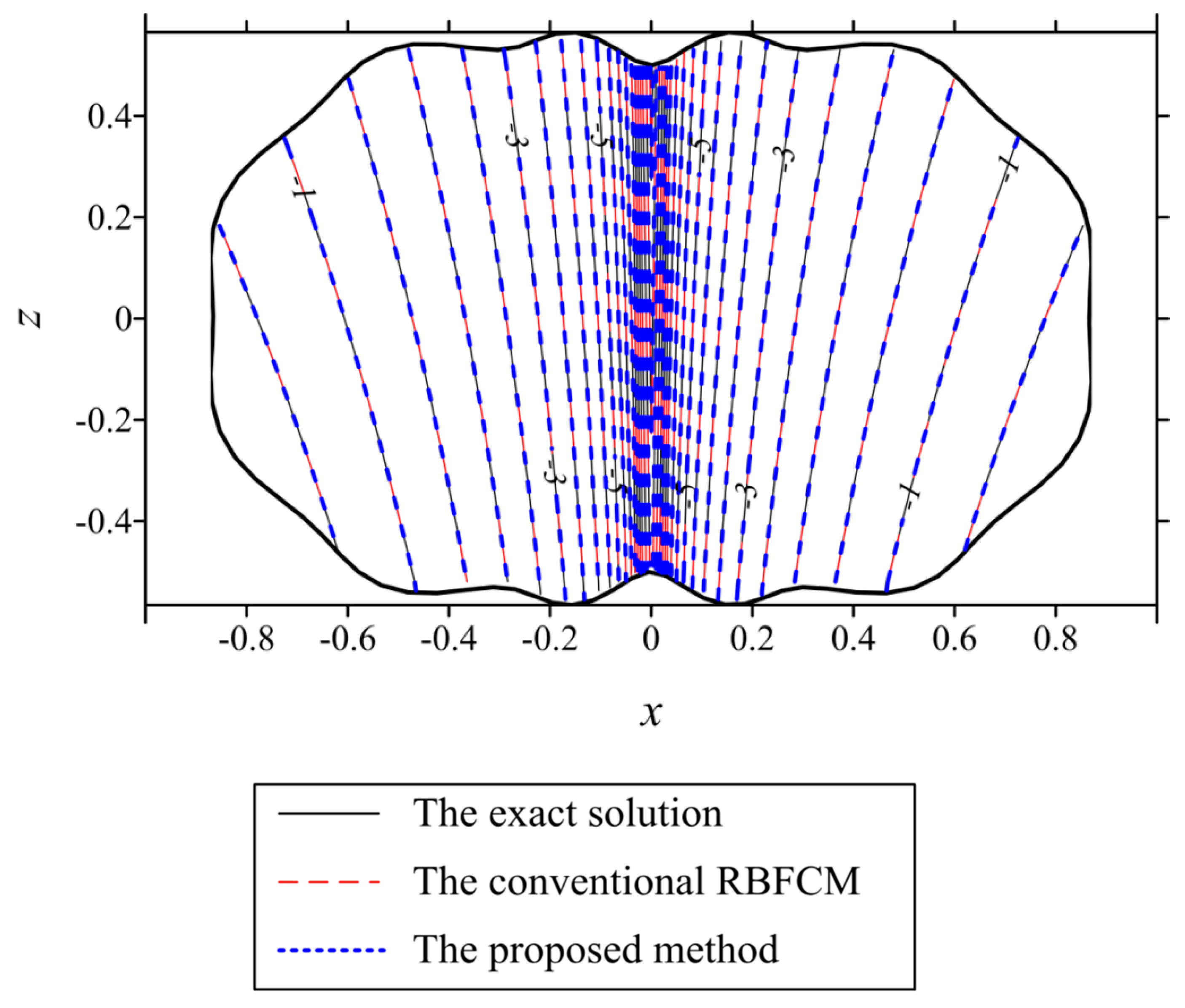
  • Several examples were conducted to verify the robustness and accuracy of our method. The results demonstrated that the proposed method using MQ and IMQ RBFs acquires more accurate results than the RBFCM, even with the optimum shape parameter. Additionally, it was found that the locations of fictitious sources were not sensitive to the accuracy.

Author Contributions

Conceptualization, C.-Y.K.; data curation, S.-M.H. and J.-E.X.; methodology, C.-Y.K. and C.-Y.L.; validation, C.-Y.L.; writing the manuscript, C.-Y.L.; editing the manuscript, C.-Y.K. and C.-Y.L. All authors have read and agreed to the published version of the manuscript.

Funding

This study was partially supported by the Ministry of Science and Technology (MOST 109-2625-M-019-007) in Taiwan.

Conflicts of Interest

The authors declare no conflict of interest.

References

  1. Hon, Y.C.; Sarler, B.; Yun, D.F. Local radial basis function collocation method for solving thermo-driven fluid-flow problems with free surface. Eng. Anal. Bound. Elem. 2015, 57, 2–8. [Google Scholar] [CrossRef]
  2. Kansa, E.J.; Hon, Y.C. Circumventing the ill-conditioning problem with multi- quadric radial basis functions: Applications to elliptic partial differential equations. Comput. Math. Appl. 2000, 39, 123–137. [Google Scholar] [CrossRef] [Green Version]
  3. Kansa, E.J. Multiquadrics—A scattered data approximation scheme with applications to computational fluid-dynamics. I Surface approximations and partial derivative estimates. Comput. Math. Appl. 1990, 19, 127–145. [Google Scholar] [CrossRef] [Green Version]
  4. Mahdavi, A.; Chi, S.W.; Zhu, H. A gradient reproducing kernel collocation method for high order differential equations. Comput. Mech. 2019, 64, 1421–1454. [Google Scholar] [CrossRef]
  5. Ku, C.Y.; Liu, C.Y.; Xiao, J.E.; Huang, W.P.; Su, Y. A spacetime collocation Trefftz method for solving the inverse heat conduction problem. Adv. Mech. Eng. 2019, 11, 1–11. [Google Scholar] [CrossRef]
  6. Mahdavi, A.; Chi, S.W.; Kamali, N. Harmonic-Enriched Reproducing Kernel Approximation for Highly Oscillatory Differential Equations. J. Eng. Mech. 2020, 146, 04020014. [Google Scholar] [CrossRef]
  7. Ku, C.Y.; Xiao, J.E. A Collocation Method Using Radial Polynomials for Solving Partial Differential Equations. Symmetry 2020, 12, 1419. [Google Scholar] [CrossRef]
  8. Cheng, A.H.-D. Multiquadric and its shape parameter—A numerical investigation of error estimate, condition number, andround-off error by arbitrary precision computation. Eng. Anal. Bound. Elem. 2012, 36, 220–239. [Google Scholar] [CrossRef]
  9. Gutmann, H.M. A radial basis function method for global optimization. J. Glob. Optim. 2001, 19, 201–227. [Google Scholar] [CrossRef]
  10. Hardy, R.L. Multiquadric equations of topography and other irregular surfaces. J. Geophys. Res. 1971, 76, 1905–1915. [Google Scholar] [CrossRef]
  11. Kansa, E.J. Multiquadrics—A scattered data approximation scheme with applications to computational fluid-dynamics. II Solutions to parabolic, hyperbolic and elliptic partial-differential equations. Comput. Math. Appl. 1990, 19, 147–161. [Google Scholar] [CrossRef] [Green Version]
  12. Chen, W.; Tanaka, M. A meshless, integration-free, and boundary-only RBF technique. Comput. Math. Appl. 2002, 43, 379–391. [Google Scholar] [CrossRef] [Green Version]
  13. Ring, M.; Eskofier, B.M. An approximation of the Gaussian RBF kernel for efficient classification with SVMs. Pattern Recognit. Lett. 2016, 84, 107–113. [Google Scholar] [CrossRef]
  14. Chen, C.S.; Karageorghis, A.; Dou, F. A novel RBF collocation method using fictitious centres. Appl. Math. Lett. 2020, 101, 106069. [Google Scholar] [CrossRef]
  15. Soleymani, F.; Barfeie, M.; Haghani, F.K. Inverse multi-quadric RBF for computing the weights of FD method: Application to American options. Commun. Nonlinear Sci. Numer. Simul. 2018, 64, 74–88. [Google Scholar] [CrossRef]
  16. Keller, W.; Borkowski, A. Thin plate spline interpolation. J. Geod. 2019, 93, 1251–1269. [Google Scholar] [CrossRef]
  17. Fasshauer, G.E.; Zhang, J.G. On choosing “optimal” shape parameters for RBF approximation. Numer. Algorithms 2007, 45, 345–368. [Google Scholar] [CrossRef]
  18. Biazar, J.; Hosami, M. Selection of an interval for variable shape parameter in approximation by radial basis functions. Adv. Numer. Anal. 2016, 2016, 1–11. [Google Scholar] [CrossRef] [Green Version]
  19. Chen, W.; Hong, Y.; Lin, J. The sample solution approach for determination of the optimal shape parameter in the Multiquadric function of the Kansa method. Comput. Math. Appl. 2018, 75, 2942–2954. [Google Scholar] [CrossRef]
  20. Ng, Y.L.; Ng, K.C.; Sheu, T.W.H. A new higher-order RBF-FD scheme with optimal variable shape parameter for partial differential equation. Numer. Heat Transf. Part B Fundam. 2019, 75, 289–311. [Google Scholar] [CrossRef]
  21. Franke, R. Recent advances in the approximation of surfaces from scattered data. In Topics in Multivariate Approximation; Academic Press: Cambridge, MA, USA, 1987; pp. 79–98. [Google Scholar]
  22. Chen, C.-S.; Karageorghis, A.; Li, Y. On choosing the location of the sources in the MFS. Numer. Algorithms 2016, 72, 107–130. [Google Scholar] [CrossRef]
  23. Li, X. On solving boundary value problems of modified Helmholtz equations by plane wave functions. J. Comput. Appl. Math. 2006, 195, 66–82. [Google Scholar] [CrossRef] [Green Version]
  24. Strack, O.D.L.; Ausk, B.K. A formulation for vertically integrated groundwater flow in a stratified coastal aquifer. Water Resour. Res. 2015, 51, 6756–6775. [Google Scholar] [CrossRef]
  25. Ku, C.Y.; Liu, C.Y.; Su, Y.; Xiao, J.E. Modeling of transient flow in unsaturated geomaterials for rainfall-induced landslides using a novel spacetime collocation method. Geofluids 2018, 2018, 1–16. [Google Scholar] [CrossRef] [Green Version]
Figure 1. The collocation scheme for the conventional radial basis function collocation method (RBFCM).
Symmetry 12 01813 g001
Figure 2. The collocation scheme for the proposed method.
Symmetry 12 01813 g002
Figure 3. The exterior source collocation scheme with different positions of the source points: (a) case A; (b) case B; (c) case C; (d) case D.
Symmetry 12 01813 g003
Figure 4. The computed maximum absolute error (MAE) for the Kansa method and the proposed multiquadric radial basis function (MQ RBF) without the shape parameter: (a) case A; (b) case B; (c) case C; (d) case D.
Symmetry 12 01813 g004aSymmetry 12 01813 g004b
Figure 5. The computed MAE for the conventional inverse multiquadric (IMQ) RBF and the proposed IMQ RBF without the shape parameter: (a) case C; (b) case D.
Symmetry 12 01813 g005aSymmetry 12 01813 g005b
Figure 6. The conventional RBFCM collocation scheme.
Symmetry 12 01813 g006
Figure 7. The proposed collocation scheme.
Symmetry 12 01813 g007
Figure 8. The computed MAE of the MQ RBF for the conventional RBFCM and the proposed method without the shape parameter.
Symmetry 12 01813 g008
Figure 9. The computed MAE of the IMQ RBF for the conventional RBFCM and the proposed method without the shape parameter.
Symmetry 12 01813 g009
Figure 10. The conventional RBFCM collocation scheme.
Symmetry 12 01813 g010
Figure 11. The proposed collocation scheme.
Symmetry 12 01813 g011
Figure 12. The computed MAE of the MQ RBF for the conventional RBFCM and the proposed method without the shape parameter. (a) D p = 0.5 . (b) D p = 10 .
Symmetry 12 01813 g012
Figure 13. Convergence analysis of the IMQ RBF for the conventional RBFCM and the proposed method without the shape parameter. (a) D p = 0.5 . (b) D p = 10 .
Symmetry 12 01813 g013
Figure 14. The collocation points of the conventional RBFCM.
Symmetry 12 01813 g014
Figure 15. The proposed collocation scheme.
Symmetry 12 01813 g015
Figure 16. The computed MAE of the MQ RBF for the conventional RBFCM and the proposed method without the shape parameter.
Symmetry 12 01813 g016
Figure 17. Convergence analysis of the IMQ RBF for the conventional RBFCM and the proposed method without the shape parameter.
Symmetry 12 01813 g017
Figure 18. Comparison of the results.
Symmetry 12 01813 g018
Table 1. A comparison of the results between the Kansa method and our approach without the shape parameter.
The Kansa MethodThe Proposed Method
(MQ RBF)
With the Optimum Shape ParameterWithout the Shape Parameter
Case ACase BCase CCase D
(c = 1.65) ( η = 4.70 ) ( η = 4.75 ) ( η = 0.15 ) ( η = 1.20 )
MAE2.06 × 10−58.58 × 10−62.98 × 10−68.11 × 10−75.15 × 10−7
RMSE6.53 × 10−74.20 × 10−71.12 × 10−75.14 × 10−82.48 × 10−8
MQ RBF, multiquadric radial basis function; MAE, maximum absolute error; RMSE, root mean square error.
Table 2. A comparisons of the results between the conventional inverse multiquadric (IMQ) RBF and the proposed IMQ RBF without the shape parameter.
The Conventional IMQ RBFThe Proposed Method
(IMQ RBF)
With the Optimum Shape ParameterWithout the Shape Parameter
Case CCase D
(c = 2.40) ( η = 1.70 ) ( η = 4.70 )
MAE1.82 × 10−53.26 × 10−74.35 × 10−7
RMSE3.26 × 10−79.63 × 10−92.19 × 10−8
Publisher’s Note: MDPI stays neutral with regard to jurisdictional claims in published maps and institutional affiliations.

