Using Machine Learning Algorithms to Estimate Soil Organic Carbon Variability with Environmental Variables and Soil Nutrient Indicators in an Alluvial Soil

Abstract

Soil organic carbon (SOC) is an important indicator of soil quality and directly determines soil fertility. Hence, understanding its spatial distribution and controlling factors is necessary for efficient and sustainable soil nutrient management. In this study, machine learning algorithms including artificial neural network (ANN), support vector machine (SVM), cubist regression, random forests (RF), and multiple linear regression (MLR) were chosen for advancing the prediction of SOC. A total of sixty (n = 60) soil samples were collected within the research area at 30 cm soil depth and measured for SOC content using the Walkley–Black method. From these samples, 80% were used for model training and 21 auxiliary data were included as predictors. The predictors include effective cation exchange capacity (ECEC), base saturation (BS), calcium to magnesium ratio (Ca_Mg), potassium to magnesium ratio (K_Mg), potassium to calcium ratio (K_Ca), elevation, plan curvature, total catchment area, channel network base level, topographic wetness index, clay index, iron index, normalized difference build-up index (NDBI), ratio vegetation index (RVI), soil adjusted vegetation index (SAVI), normalized difference vegetation index (NDVI), normalized difference moisture index (NDMI) and land surface temperature (LST). Mean absolute error (MAE), root-mean-square error (RMSE) and R² were used to determine the model performance. The result showed the mean SOC to be 1.62% with a coefficient of variation (CV) of 47%. The best performing model was RF (R² = 0.68) followed by the cubist model (R² = 0.51), SVM (R² = 0.36), ANN (R² = 0.36) and MLR (R² = 0.17). The soil nutrient indicators, topographic wetness index and total catchment area were considered an indicator for spatial prediction of SOC in flat homogenous topography. Future studies should include other auxiliary predictors (e.g., soil physical and chemical properties, and lithological data) as well as cover a broader range of soil types to improve model performance.

1. Introduction

Globally, soils of the humid tropics have received overwhelming acceptance for agriculture. However, these soils in southeastern Nigeria have the potential that could be exploited for crop production. Unfortunately, they are both highly weathered and leached soils formed on alluvial deposits under excessive rainfall and high-temperature conditions [1,2]. This soil like other soils weathers through the actions of environmental conditions (i.e., topography, and other soil-forming factors) to give the soil their genetic properties (e.g., soil pH, texture, clay, CEC, exchangeable cations) [3]. Soil texture, nutrient status, and mineralogical properties of alluvial deposits bear the imprints of quartz oxides, which are not rich in most plant growth nutrients [4]. This status gives low crop yield if there is no application of appropriate nutrient amendments. For example, the yield of fresh fruit bunches (FFB) is estimated at 3–5 t·ha⁻¹ from University of Calabar Teaching and Research Farm; under alluvial deposits soil is far less than the national average of 8–12 FFB t·ha⁻¹ and world-record yields of 25–35 t·ha⁻¹ in Malaysia [5].

Soil organic carbon (SOC) is an essential indicator of soil quality, and directly determines soil fertility and plant productivity [5]; it plays a significant role in supplying nutrients to the soil and in the formation of improved soil structure. In previous years, several soil researchers have reported variability of SOC in different ecological zones of the world [6,7,8]. These studies are in line with the different assumptions, including the fact that variation in crop yield within a given field reflects variation in SOC [9]. Their studies further explained that in order to achieve appropriate soil nutrient management for uniform crop yield, it is necessary to know where the low SOC, as well as soil nutrients, reside within a given field, and how much carbon or soil nutrient is present. This is essentially the importance of quantitative soil mapping. The accurate and up-to-date information obtained in the process ensures the application of site-specific nutrient management to match spatially variable conditions.

Variability of soil nutrients is a significant constraint for sustainable crop production due to the resulting non-uniformity of output across different sections of the field. One way of minimizing heterogeneity in the soil resulting in different crop yields is through digital soil mapping (DSM), but it is often constrained by within-site variability [10]. These issues became the target of a site-specific cropping system, otherwise known as precision agriculture. The technique of precision agriculture can delineate sites for specific management. Precision agriculture has now been developed to spatially varied nutrients and soil properties within a field relying on geospatial technologies and utilizing soil properties, remote sensing data, digital elevation model (DEM), micro-climatic data, and geology [11]. Precision agriculture allows farm managers to manage within-field variability to maximize the cost–benefit ratio of the proposed crop enterprise. Besides that, specific landscape attributes control the spatial distribution of SOC coupled with the interactive action of soil-forming factors [3,12].

In agro-ecosystems, the spatial distribution of soil properties is affected by natural ecological processes influenced by many factors, including climate, soil type, topography, and land use. It thus becomes a challenge to accurately model SOC at farm scales [10,13] over a broader area that spans several kilometres without taking into consideration these factors. Before the advent of geospatial technologies, the spatial distribution of soil properties including SOC was assessed from conventional soil surveys and laboratory analyses of collected soil samples utilizing classical statistics; an approach that is tedious, time-consuming, and expensive. The traditional soil survey method could not provide detailed information about soil variation required for many environmental applications. Thus, alternative approaches are needed. As an alternative, the digital soil mapping (DSM) technique was developed and became one focus of soil and environmental science. Under the framework of the DSM, several geostatistics prediction methods, as found in John et al. [9], have been developed to predict the spatial distribution of soil properties.

Through the advances in technology, there is a comprehensive application of machine learning algorithms such as multiple linear regression (MLR), artificial neural network (ANN), support vector machine (SVM), decision tree, cubist regression, and random forests in soil studies using auxiliary environmental data [8,14].

Environmental auxiliary data such as digital elevation models (DEM), remote sensing, climatic data, and geology have been combined via predictive models to estimate soil properties. A large number of existing DEM data sets (e.g., SRTM DEM and Aster GDEM) [6,15,16] has been used to extract terrain attributes (e.g., elevation, slope, aspect, topography wetness index) as predictors for predicting soil properties. Remote sensing images, on the other hand, have also served as excellent data for both qualitative and quantitative study of soil properties, including SOC [7,8,15]. Previous studies on predicting SOC primarily utilized multi-spectral optical sensors, including Landsat [6,8], MODIS [17], SPOT [18], RapidEye [19], Landsat and MODIS [15], and Landsat and ALOS PALSAR [20]. Remote sensing data provides a cost-effective, reproducible, and spontaneous approach to quantifying SOC variability [21]. This technique is achieved through the correlation between soil reflectance and SOC. In [22] it is reported that the increase in SOC is inversely proportional to an overall decrease in reflectance in the visible (Vis, 400–700 nm), near-infrared (NIR, 700–1400 nm), and shortwave infrared (SWIR, 1400–2500 nm) regions of the electromagnetic spectrum (McMorrow et al. [23,24]).

Fathololoumi et al., [25] worked on improved digital soil mapping with multitemporal remotely sensed satellite data fusion in Iran using random forest (RF) and cubist models. Their results showed that the cubist model exhibited greater accuracy than RF in the modeling of SOC. While in the high-resolution mapping of soil properties using remote sensing variables in southwestern Burkina Faso (studies conducted by Forkuor et al. [19]), RF performed better in the prediction of SOC. In addition, in the prediction and mapping of soil organic carbon using MLA in Northern Iran by Emadi et al. [15], the deep neural network (DNN) model was reported as a superior algorithm with the lowest prediction error and uncertainty. Bian et al. [7] utilizes multiple stepwise regression (MSR), boosted regression trees (BRT) model, and boosted regression trees hybrid residuals kriging (BRTRK) to model SOC in northeastern coastal areas of China. Similarly, Taghizadeh-Mehrjardi et al. [6] use the artificial neural network (ANN), support vector regression (SVR), k-nearest neighbour (kNN), random forest (RF), regression tree model (RT), and genetic programming (GP) to predict SOC. Their study recommended the combination of ANN and equal-area spline functions for predicting SOC spatial distribution in the Baneh region of Iran.

Despite the acceptability of MLA in DSM, few or no studies have considered the incorporation of soil nutrient indicators and environmental data in modeling SOC in southeastern Nigeria and the world at large. Additionally, the Nigeria environment is yet to get acquainted with the modeling program involving MLA in soil mapping, and no feasible study has been carried out elucidating this approach, despite the region’s active engagement in agriculture production. Consequently, a fundamental knowledge gap remains, hindering the ability of farm managers and agronomists to improve the land and soil quality. Furthermore, we hypothesize that in flat terrain configuration, soil nutrient indicators play many roles in explaining SOC distribution to ancillary environmental data. Therefore, in this study, we applied five machine learning algorithms (RF, Cubist, ANN, MLR, and SVM) to estimate the SOC variability in a flat alluvial terrain condition with environmental variables and soil nutrient indicators known to influence SOC variability in the alluvial deposit of Calabar, Nigeria.

2. Materials and Methods

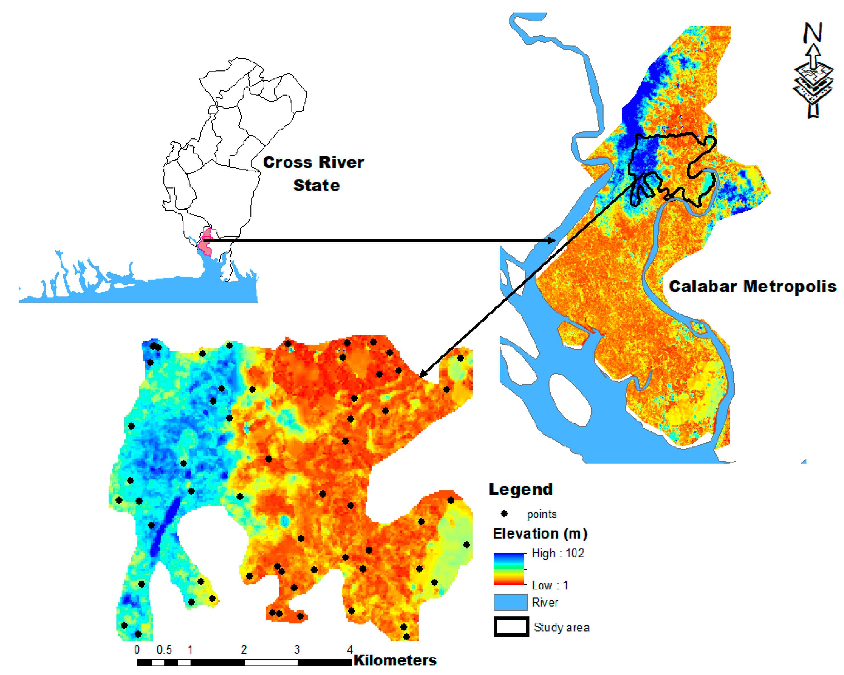
2.1. Description of the Study Area

The study was conducted in Calabar, Cross River State. The study area extends from latitudes 4°57’ N–5°00’ N and longitude 8°19’ E–8°24’ E (Figure 1), and spreads over an area of approximately 60 km² with an elevation range of 1 to 102 m above sea level. The area is characterized by a humid tropical climate with distinct wet and dry seasons. This area receives average annual rainfall exceeding 2500 mm per annum; and the average minimum and maximum temperatures of this area are about 22 °C and 30 °C, respectively, with a mean relative humidity of 83% [26]. The principal crops grown in the area include maize, sugar cane, cassava, groundnut, oil palm and vegetable crops (okra, Telfairia occidentalis, pepper, waterleaf, Amaranthus cruentus, etc.). The soils of the study area are developed on coastal plain sand parent material [27]. They are characterized by udic moisture regime and isohyperthemic temperature regimes, respectively [28]. Furthermore, according to USDA soil taxonomic classification, the soil order of the region is overwhelmingly Ultisols, and the soil is classified as Typic kandiudults [29].

2.2. Soil Sampling Regime and Laboratory Analysis

A total of sixty (n = 60) composite soil samples were collected at a depth of 0–30 cm with the aid of a soil auger at a sampling density of one sample per 3.3 m² and were thoroughly mixed in a Ziploc bag to obtain a homogenized sample. The soil sampling at 0–30 cm is the depth of the tillage zone. We sampled to this depth because there is no significant accumulation of SOC beyond 30 cm in the alluvial deposit. The sampling was aided by a hand-held global positioning system (GPS) (Garmin eTrex 10). These samples were adequately labeled and transported to the laboratory for analysis.

The samples were air-dried, ground, and passed through a 0.5 mm sieve. The SOC was determined by the standard Walkley–Black wet oxidation method using acid dichromate (K₂Cr₂O7) solution, as outlined in Udo et al. [30]. At the same time, effective cation exchange capacity (ECEC), base saturation, calcium (Ca), magnesium (Mg), and potassium (K) were obtained by standard laboratory procedure prescribed by Udo et al. [30]. These analyses were carried out at the University of Calabar Soil Science Department Laboratory. The soil nutrient indicators used as part of the explanatory variables was estimated from the already laboratory-measured soil properties, for example, Ca²⁺ to Mg²⁺, K⁺ to Mg²⁺ and K⁺ to Ca²⁺ ratios were calculated using their representative basic cations; furthermore, in this study, they are represented as Ca_Mg, K_Mg, K_Ca, respectively.

2.3. Environmental Covariates

Environmental covariates were derived from both the digital elevation model (DEM), obtained at the spatial resolution of 30 m from ASTER GDEM, and Landsat 8 operational land imager (OLI) and a thermal infrared sensor (TIRS) acquired at https://earthexplorer.usgs.gov. DEM was processed using System for Automated Geoscientific Geographical Information System (SAGA-GIS) software terrain analysis toolbox.

The Landsat 8 Operation Land Imager (OLI) remote sensing data Path 187/Row 57 was acquired 2 January 2018 (growing season) with a cloud cover of 6.31% and SCENE_ID “LC81880562018361LGN00”, and used to derived spectral indices and land surface temperature (LST) (

Table 1. Environmental covariates for soil organic carbon prediction.

Environmental Covariates	Variable	Description
Landsat 8 OLI	b3	Green, 0.525–0.600 μm
	b4	Red, 0.630–0.680 μm
	b5	NIR, 0.845–0.885 μm
	Clay index (CI)	$\mathrm{CI}=\frac{\mathrm{SWIR}1}{\mathrm{SWIR}2}$
	Iron index	$\mathrm{Iron}\mathrm{index}=\frac{\mathrm{Red}}{\mathrm{Blue}}$
	Normalized Difference build-up Index (NDBI)	$\mathrm{NDBI}=\frac{(\mathrm{SWIR}–\mathrm{NIR})}{(\mathrm{SWIR}+\mathrm{NIR})}$
	Ratio Vegetation Index (RVI)	$\mathrm{RVI}=\frac{\mathrm{NIR}}{\mathrm{RED}}$
	Soil Adjusted Vegetation Index (SAVI)	$\mathrm{SAVI}=\frac{(\mathrm{NIR}–\mathrm{RED})}{(\mathrm{NIR}+\mathrm{RED}+\mathrm{L})}\times (1+\mathrm{L})$
	Normalized Difference Vegetation Index (NDVI)	$\mathrm{NDVI}=\frac{(\mathrm{Band}5–\mathrm{Band}4)}{(\mathrm{Band}5+\mathrm{Band}4)}$
	Normalized Difference Moisture Index (NDMI)	$\mathrm{NDMI}=\frac{(\mathrm{NIR}–\mathrm{SWIR})}{(\mathrm{NIR}+\mathrm{SWIR})}$
	Land surface temperature (LST)	$LST=\frac{\mathrm{BT}}{\left\{1+\left[(\lambda BT/\rho )ln\epsilon \right]\right\}}$
ASTER GDEM	Elev	Elevation
	PCurv	Plan curvature
	TCA	Total catchment area
	CNBL	Channel Network base level
	TWI	Topographic wetness index

). The images contain nine spectral bands with a resolution of 30 m (multi-spectral), 15 m (panchromatic), and 100 m (TIRS bands 10 and 11), resampled to 30 m. The Landsat images were geometrically corrected and projected to a World Geodetic System 1984 (WGS 84) into a Universal Transverse Mercator (UTM) Zone 32N coordinate system. Detailed specifications and preprocessing method of the Landsat 8 OLI images to obtain surface reflectance images can be found in Roy et al. [31]. The area of interest (AOI) was demarcated in the satellite images with the help of the polygon feature using the ArcGIS 10.8 software (ESRI, Redlands, USA) environment.

Retrieval of land surface temperature (LST) from thermal infrared sensor (TIRS) band 10 was carried out according to the following sequence of steps. The first step involves the conversion of the Digital number (DN) of the thermal infrared band into spectral radiance ($L\lambda$) as presented in Equation (1):

$$L\lambda =M_L\times Q_{cal}+A_L$$

(1)

where, $L\lambda$ = atmospheric SR in watts/(m² × srad × μm), $M_L$ = band-specific multiplicative rescaling factor from the metadata, $Q_{cal}$ = corresponds to band 10, $A_L$ = band-specific additive rescaling factor from the metadata.

The second step involves the conversion of spectral radiance to brightness temperature in Celsius.

$$\mathrm{BT}=\frac{{\mathrm{K}}_2}{\ln \left(\frac{{\mathrm{K}}_1}{L\lambda }+1\right)}-273.15$$

(2)

where, BT is the satellite brightness temperature in Celsius, and K₁ and K₂ represent thermal conversion from the metadata.

$$L\lambda =\mathrm{spectral}\mathrm{radiance}\mathrm{at}\mathrm{the}\mathrm{sensor}\prime \mathrm{s}\mathrm{aperture}[\mathrm{W}/({\mathrm{m}}^2\mathrm{sr}\mathsf{\mu }\mathrm{m}\left)\right]$$

The next step was the calculation of the normalized difference vegetation index (NDVI), the proportion of vegetation (P_V), which is highly related to the NDVI, and emissivity (ε), which is related to the P_V.

$$\mathrm{NDVI}=\frac{(\mathrm{Band}5 -\mathrm{Band}4)}{(\mathrm{Band}5+\mathrm{Band}4)}$$

(3)

Estimation of the proportion of vegetation P_V

$$P_V={\left[\frac{\mathrm{NDVI} -{\mathrm{NDVI}}_{\min }}{{\mathrm{NDVI}}_{\max } -{\mathrm{NDVI}}_{\min }}\right]}^2$$

(4)

Estimation of land surface emissivity (LSE)

$$\epsilon =0.004\times P_V+0.986$$

(5)

Calculation of land surface temperature

$$LST=\frac{\mathrm{BT}}{\left\{1+\left[(\lambda BT/\rho )ln\epsilon \right]\right\}}$$

(6)

where LST is Celsius, BT is the at-sensor brightness temperature in Celsius, λ (10.8 μm) is the wavelength of the emitted radiance: ρ = h × c/σ = 1.438 × 10⁻² mK, σ is the Stefan–Boltzmann constant, h is Planck’s constant, c is the velocity of light, and ε is the land surface emissivity (LSE). The computation of other covariates from Landsat 8 OLI is shown in Table 1.

2.4. Machine Learning Techniques

In this study, five ML algorithms, including random forest (RF), cubist regression, artificial neural networks (ANN), support vector machine (SVM), and multiple linear regression, were chosen. A brief description of the ML techniques used in this study are presented as follows:

2.4.1. Random forest

Random forests (RF) is an ensemble of classification and regression trees (CART). This MLA was developed by Breiman [32] and is said to be as accurate as or better than adaptive boosting, yet computationally faster [33,34]. RF algorithm can handle both continuous and categorical variables. The RF algorithm is quite robust to noise in predictors and thus does not require a pre-selection of variables [35]. In RF, two hyperparameters are usually modified by users to regulate the complexity of the models, including (a) the number of trees (or iterations) (ntree), which also corresponds to the numbers of decision trees; random forests will overfit if the number is too large; (b) and mtry depicts the number of indicators that are randomly sampled as candidates at each split. In this case study, we will tune two parameters, namely the ntree and the mtry parameters that have the following effect on our random forest model.

In this present study, the model performance is obtained from each combination of the hyperparameters tuning with the grid search method [36] with cross-validation (CV) methods. K-fold CV is one of the extensively employed CV methods in machine learning and there is no definite rule for selecting the value of k. However, a value of k = 5 or 10 is ubiquitous in the field of applied machine learning and in this present study, we adopted this k = 10 in five repetitions. This was executed to avoid bias in data selection during RF hyperparameters tuning. According to Rodriguez [37], the bias of an accurate estimate will be smaller when the number of folds is either five or ten.

2.4.2. Cubist Regression

The cubist model was developed by Quinlan [38] as a rule-based model which is an extension of the M5 tree model. According to Kuhn [39], the model structure consists of a conditional component—or piecewise function acting as a decision tree, coupled with multiple linear regression models. The trees are reduced to a set of rules which are eliminated via pruning or combined for simplification. The main benefit of the cubist method is to add multiple training committees and boosting to make the weights more balanced [38,39,40]. The cubist model adds boosting with training committees (usually greater than one) which is similar to the method of “boosting” by sequentially developing a series of trees with adjusted weights. The number of neighbours in the cubist model is applied to amend the rule-based prediction [39]. This model was implemented in R with tuning two hyper-parameters: neighbors (Instances) and committees (Committees). These two parameters are the most likely parameters to have the largest effect on the final performance of the cubist model. Cubist followed a similar approach in RF

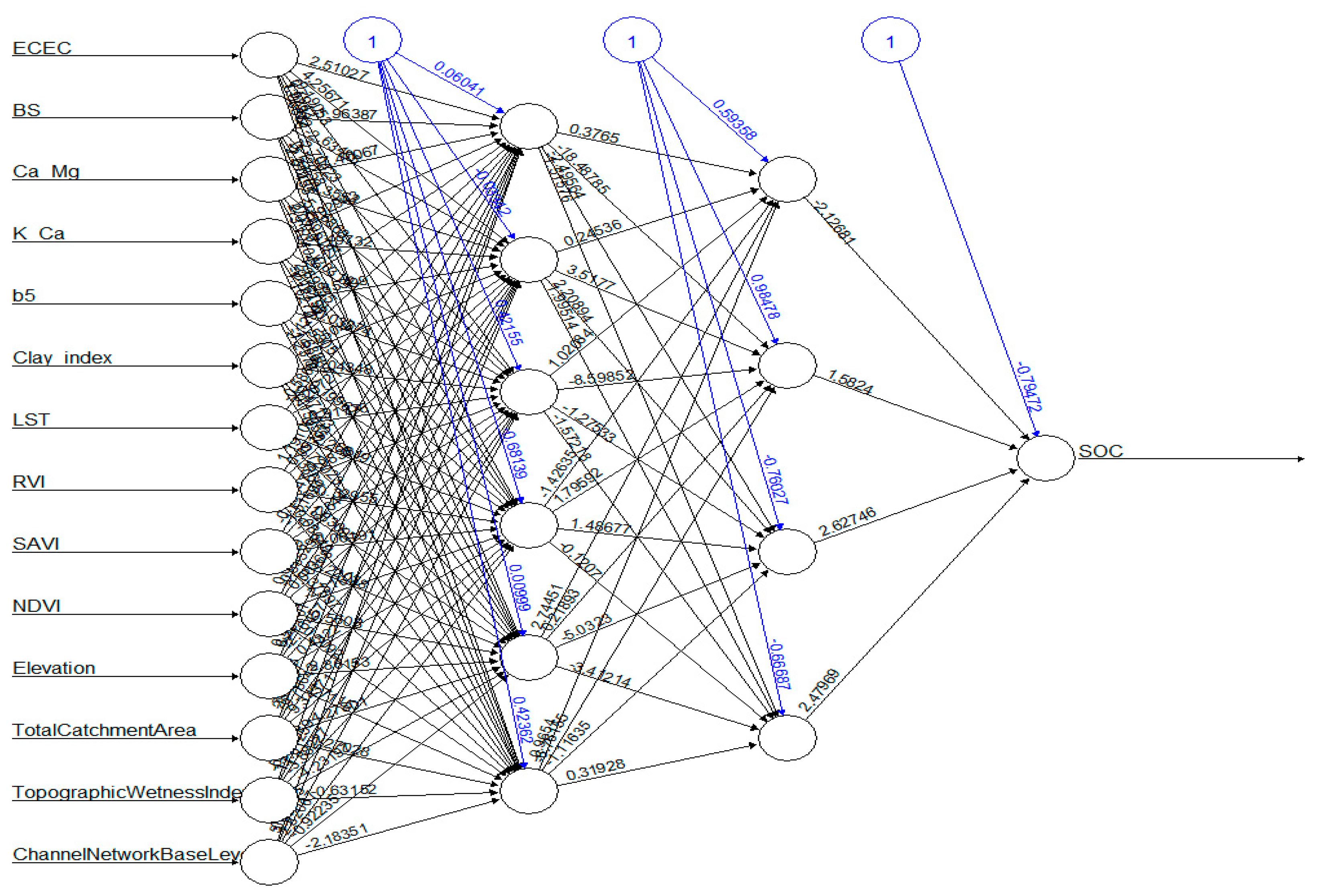
2.4.3. Artificial Neural Network

In predictive modeling and forecasting, as well as nonlinear and impermanent time series of processes where there is no exact solution and clear relationship to recognize and describe them, artificial neural networks have shown good performance. The frequently used ANN model is referred to as the multilayer perceptron (MLP). This model is occasionally used as a substitute for a feed-forward network. The MLP requires a well-known output so that to learn and train the network; this type of neural network is referred to as a supervised network. MLP produces a model that plots the input to the output using training data so that subsequently, the model is applied to predict the output when it is unknown. In the present study, and after some preliminary tests to choose the model, multilayer feed-forward back-propagation ANN was applied [41]. The ANN models are well adapted for modeling nonlinear behaviour. They have the capacity of learning for complex relationships between multiple inputs and output variables. The ANN model was run in R using the package “nnet.” The best structure for the ANN model was obtained by changing the size (number of units in the hidden layer).

2.4.4. Multiple Linear Regression

Multiple linear regression (MLR) is a machine learning algorithm applied to regress a target variable that is SOC in this study against some selected covariates (e.g., environmental variables and soil nutrient indicators). In soil spatial prediction functions, MLR is a least-squares model where a targeted soil property is predicted from selected explanatory variables. So, in this present research, a linear relationship was established for SOC (response variable) using the explanatory variables. A simple MLR equation is presented in Equation (1).

$$y=a+{\displaystyle \sum }_{i-1}^n{b}_i\times x_i \pm {\epsilon }_i$$

(7)

where $n$ = number of predictors; $y$ = response variable (SOC); $x_i$ = explanatory variables or predictors (environmental and soil nutrient indicators variables); $a$ = intercept (constant term); $b_i$ = partial regression coefficients; ${\epsilon }_i$ = the model’s error term (also known as the residuals).

This was automatically implemented in R using the k = 10 folds CV in five repetitions. In addition, the tuning parameter “intercept” was held constant at a value of true

2.4.5. Support Vector Machine (SVM)

Support vector machine (SVM) is a machine learning algorithm that produces an optimal separating hyperplane to differentiate classes that overlap and are not separable in a linear way. It was originally developed for classification purposes; however, it can also be used for regression problems [42]. In this study, SVM for regression (SVR) was implemented. SVR is a kernel-based learning regression method that was proposed by Cherkassky [43]. It is based on the computation of a linear regression function in a multidimensional feature space. Hence, modeling a linear regression hyperplane for nonlinear relationships is possible with the feature space. Two forms of SVM regression, namely, “epsilon (ε)-SVR” and “nu (v)-SVR,” are commonly used in the SVM model. The original SVM formulations for regression (SVR) use parameter cost (c) and epsilon (ε) to apply a penalty to the optimization for points that are incorrectly predicted. Several studies, including Siewert [44] and Zhang et al. [45] have utilized SVR in environmental monitoring studies to predict SOC. In SVM regression, the Gaussian Radial Basis Function (RBF) kernel was applied. We employed the RBF kernel to obtain an optimal SVM regression model which is important to obtain the best set of penalty parameters C and kernel parameters gamma (γ) for the SOC training datasets. In the present study, we evaluated the training set and then tested the model performance on the validation set.

2.5. Data Scaling and Partitioning

The dataset used for modeling (n = 60) was scaled to a range between 0 and 1, indicating the lowest and the highest value, respectively. To evaluate the suitability of the different models for SOC prediction, a completely random technique was applied to divide the dataset into training (80%), and test (20%) datasets. Each model was fitted using the train data while the test data was used for validation. A 10-fold cross-validation was applied to the training dataset for each of the models used in the study and repeated five times. This and all modeling were performed in R software [46].

2.6. Model Validation and Accuracy Assessment

From the pool of twenty (22) SOC predictors, only the significant predictors (p-value < 0.1) were selected to build a prediction model. This was established using a simple correlation matrix. The models selected for this study were evaluated for their performance. The models were trained with 80% of the dataset (i.e., 48 observation points) and the validation set was tested by the remaining 20% of the dataset (i.e., 12 observation points). Mean absolute error (MAE), root-mean-square error (RMSE) and R² were used to determine the model performance according to the following equations:

$$MAE=\frac{1}{n}{\displaystyle \sum _{i=1}^n|SOC\left(X_i\right)}-SOC\left({\widehat{X}}_i\right)|$$

(8)

$$RMSE(\%)=\sqrt{\frac{1}{n}{\displaystyle \sum _{i=1}^n{[SOC\left(\widehat{X_i}\right)-SOC\left(X_i\right)]}^2}}$$

(9)

$$R^2(\%)=1-\frac{{\sum }_i{[SOC\left(X_i\right)-SOC\left({\widehat{X}}_i\right)]}^2}{{\sum }_i{[SOC\left(X_i\right)-SOC\left({\widehat{X}}_i\right)]}^2}$$

(10)

where n = the size of the observations, SOC($X_i$) = measured response and SOC($\widehat{X_i}$) = predicted response values, respectively, for the i-th term observation, SOC($\overline{X_i}$) being the average of the response variable. Furthermore, a good model prediction was expected to have low MAE and RMSE as well as an R² value close to 1. Li et al. [47] proposes a classification criterion for R² values: R² < 0.50 (unacceptable prediction), 0.50 ≤ R² < 0.75 (acceptable prediction) and R² ≥ 0.75 (good prediction). The same criterion was applied in the current study.

3. Results and Discussion

3.1. Descriptive Statistics

The descriptive statistics of the SOC of the study site are shown in

Table 2. Descriptive statistics of soil organic carbon (SOC). ⟵

	n	Mean	Median	SD	Min	Max	1st Quartile	3rd Quartile	CV
⟶ % ⟵
SOC	60	1.62	1.38	0.76	0.32	3.10	1.0	2.24	47

. SOC value ranged from 0.32 to 3.10% with the mean of 1.62% and coefficient of variation (CV) of 47%. According to the classification proposed by Wilding and Drees [48], SOC samples indicated high variability (CV > 35%) which may be attributed to random factors such as environmental factors and measurement errors [49,50]. Using Landon [51] rating for tropical soils, the SOC of the study was generally low. The low SOC in the soil is consistent with the findings by Akpan-Idiok and Ogbaji [29] and Taghizadeh-Mehrjardi et al. [6] in Cross River State, and also with that of Bednář and Šarapatka [52] in the Czech Republic. The low SOC content may be attributed to the disturbance of the topsoil (0–30 cm) during tillage activities in preparation of the site for planting, in addition to high temperature, and high erodibility of the soils resulting from high rainfall intensity experienced in the area [1].

Furthermore, intensive cultivation depletes soil organic matter accumulation, and in turn lowers SOC content through the increase in decomposition rate generated by the change in the aggregate structure of the soil due to the cultivation and mixing effect of tillage [53]. The current study is supported by the plausible reasons that intensive cultivated systems reduce SOC contents due to increased mineralization created through soil surface disturbance [54,55,56,57].

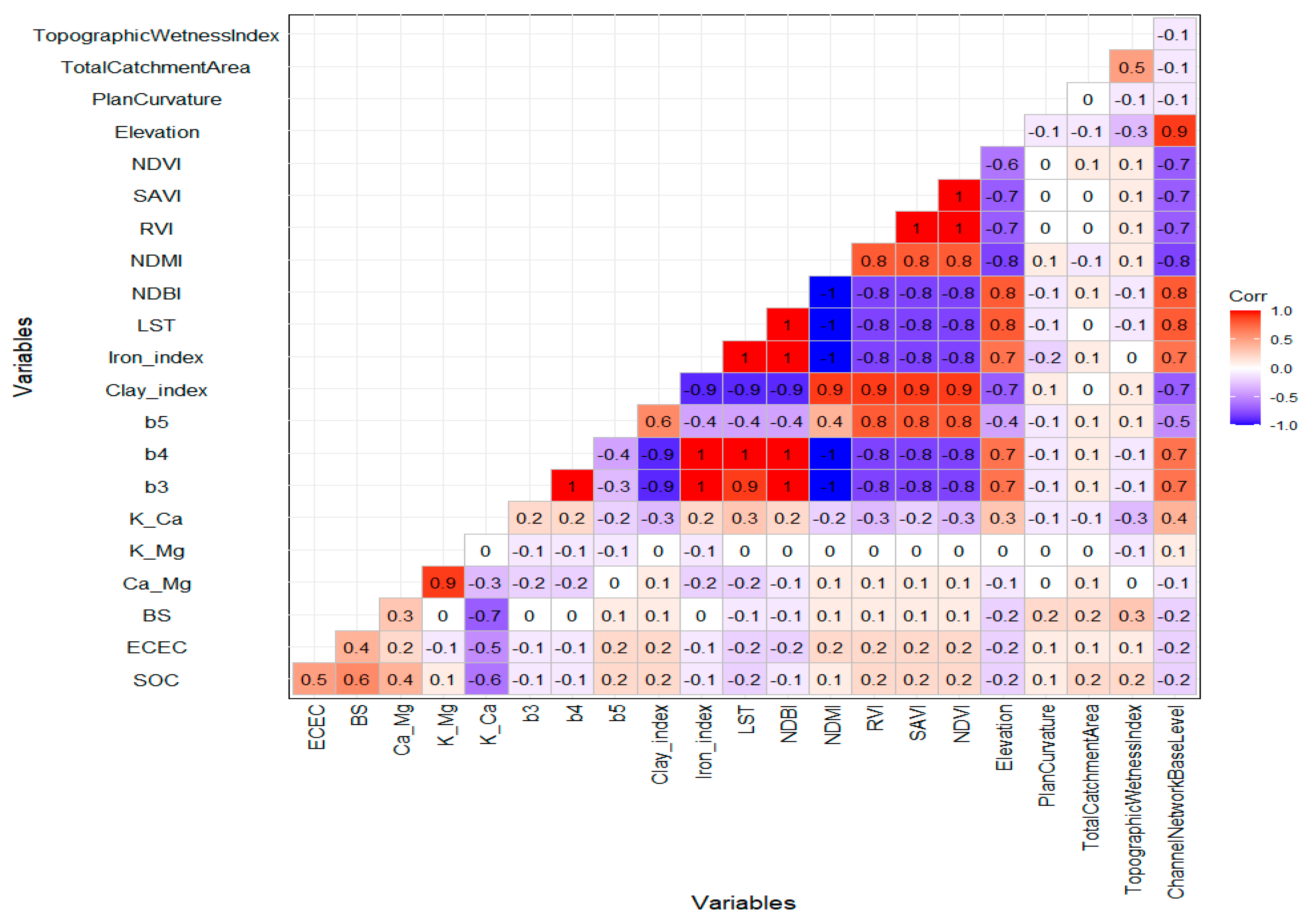
3.2. Correlation between SOC and Environmental Variables and Soil Indicators

Figure 2 shows the correlation between SOC and environmental variables and soil indicators. SOC was weakly correlated with b5 (r = 0.2), clay_index (r = 0.2), LST(r = −0.2), RVI (r = 0.2), SAVI (r = 0.2) and NDVI (r = 0.2) obtained from Landsat satellite imagery. Similarly, SOC was weak but significantly correlated with elevation (r = −0.2), total catchment area (r = 0.2), topographic wetness index (r = 0.2) and channel network base level (r = 0.2) derived from digital elevation model (DEM). The result obtained here showed that environmental variables obtained from Landsat imagery gave a poor relationship with SOC in a flat topographical system. Environmental variations in areas with a small range of topography, such as plains, are usually very small [20]. This factor including but not limited to the time of acquiring spaceborne data and intensive crop cultivation utilizing chemical fertilizers in the area, could be responsible for the low correlation between SOC and NDVI in the studied soil. Furthermore, NDVI may only show a high contribution to SOC when the crops are producing more crop biomass. The result is supported by the findings of Florinsky et al. [58] and Mosleh et al. [10].

Additionally, the effect of environmental variables for SOC in this low-relief area was weakly correlated, and the spatial variability of SOC cannot be obtained by total dependence on both terrain and remote sensing parameters. On the other hand, a good relationship was obtained between SOC and soil nutrient indicators. That is, SOC was strongly correlated with ECEC (r = 0.50), base saturation (BS) (r = 0.60), K_Ca (r = −0.60) and moderately correlated with Ca_Mg (r = 0.40). ECEC and BS increase with an increase in organic matter accumulation [56,59]. The observation between soil nutrient indicators (Ca_Mg and K_Ca) and SOC represents that the accumulation of organic materials in the soil surface may increase or decrease Ca, Mg and K in the soil.

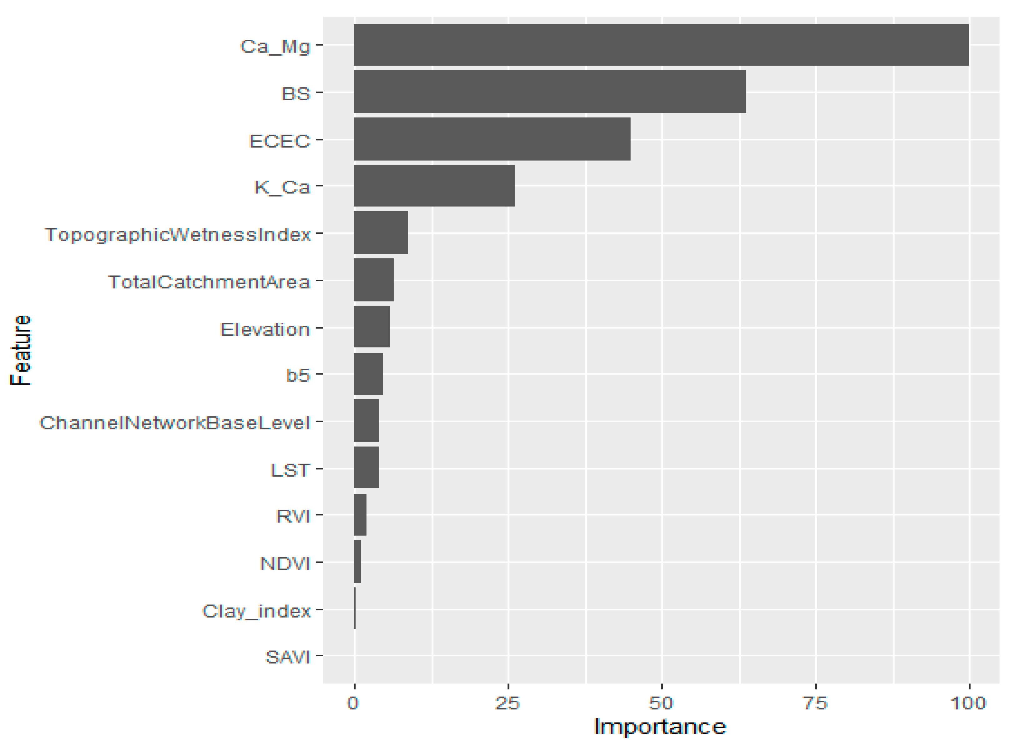
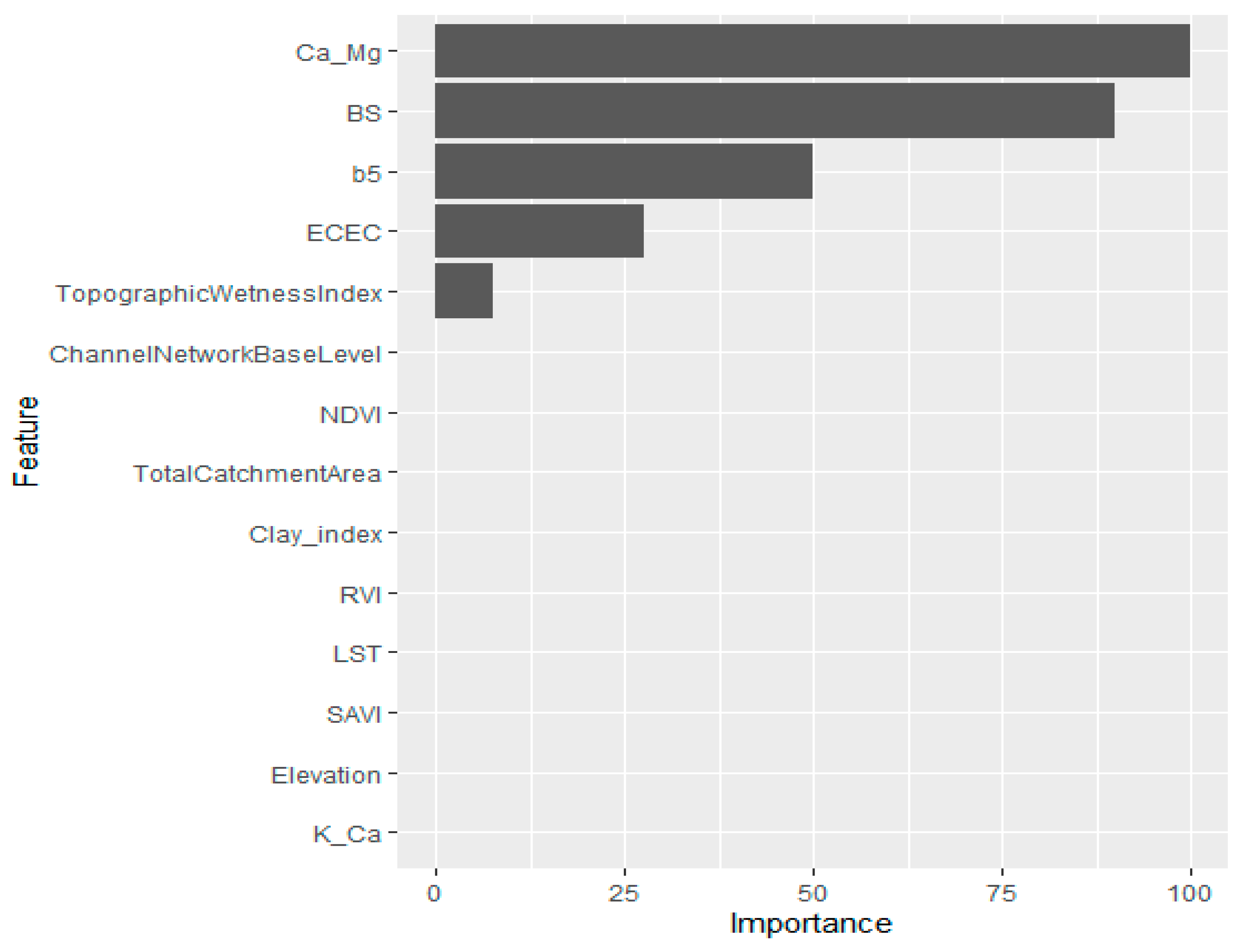
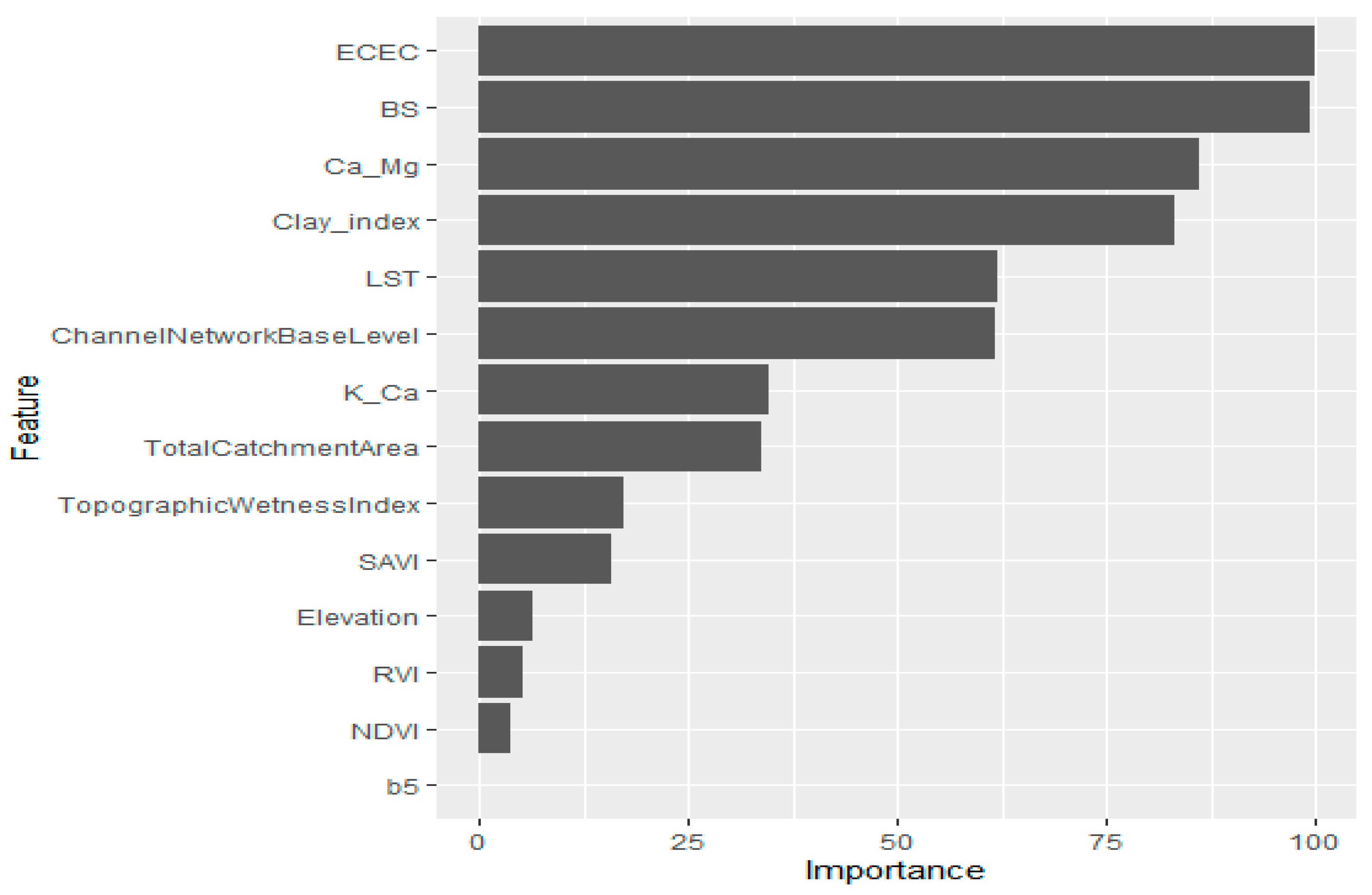
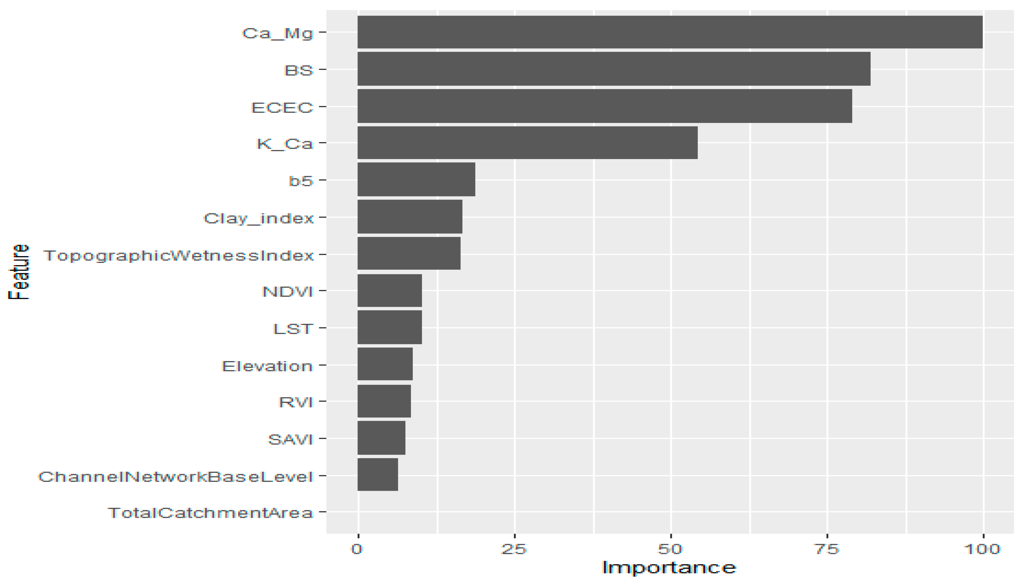
3.3. Modeling Approach and Variables of Importance in the Individual Models

The optimum selection strategy of covariates is that the correlation between the covariates and the response variable is significant or high, and the covariates are obtained effortlessly [16]. Among 22 explanatory variables, only 14 of the explanatory variables that showed a significant correlation with SOC were selected (p < 0.01). These variables were b5, clay_Index, LST, RVI, SAVI, NDVI, elevation, total catchment area, topographic wetness index, channel network base level, ECEC, BS, K_Ca and Ca_Mg.

For RF prediction model, as shown in Figure 3, Ca_Mg, BS, ECEC, K_Ca, topographic wetness index best predictors to explain the variability of SOC in a flat terrain system. In addition, the result reveals that the soil nutrient indicators contribute much more compared to environmental variables in estimating SOC in a flat topographic system.

Similarly, the environmental variables show their inability to contribute to SOC prediction in low relief conditions. This result is supported by Mosleh et al. [10]. They conducted a study in Iran and stated that environmental variables are not essential relative variables in low relief conditions. Furthermore, Solly et al.’s [60] report supported this current study through the study done in Switzerland on the preservation of SOC using cation exchange capacity plus mean annual temperature, mean annual precipitation, and leaf area index. Their study concludes that soil physical and chemical properties serve as better predictors in a homogenous terrain. Similar conclusions were reported by Song et al. [61], who noted that local environmental attributes play a less significant role than other predictors on a flat terrain system. Li et al. [62] inferred that environmental attributes could capture large-scale influences of soil transport but not those occurring at a flat topographic condition. Thus, the over-employment of environmental factors in small-scale flat terrain areas reduces the prediction accuracy and increases the calculation complexity.

Presented in Figure 4 is the cubist model prediction using the calibration set. The plot showed a similar output with RF. Ca_Mg was the best predictor with BS, b5, ECEC and topographic wetness index following. Similarly, in the artificial neural network model (Figure 5), the best predictor is ECEC, closely followed by BS, Ca_Mg, K_Ca and b5. Landsat near-infrared band (b5) gave a 50% contribution to SOC prediction, and this is reverse to a region with strong undulating topography as reported by Emadi et al. [15] for complex terrain. This output is also similar to the previous models and still powerfully reveals the dominance of soil nutrient indicators in the estimation of SOC.

According to Figure 6, MLR presented high relative importance (>50%) of the explanatory variables. ECEC was the best predicting variable and then followed by BS, Ca_Mg, clay_index and LST. In Figure 7, the support vector machine model followed a similar pattern as compared to other models (i.e., RF and cubist). That is, soil nutrient indicators do a better job in estimating SOC to environmental variables in flat terrain condition under small-scale.

Support vector machine model yielded Ca_Mg as the best predictor and then followed by BS, ECEC, K_Ca, b5, clay_index and topographic wetness index. The percentage contribution by topographic wetness index to SOC prediction is above the value reported by Emadi et al. [15]. However, they follow a similar pattern in that they contribute a little amount in SOC variability in low relief conditions. In all the five MLAs, NDVI made little or no contribution to SOC estimation, and this is contrary to what is experienced in more complex terrain.

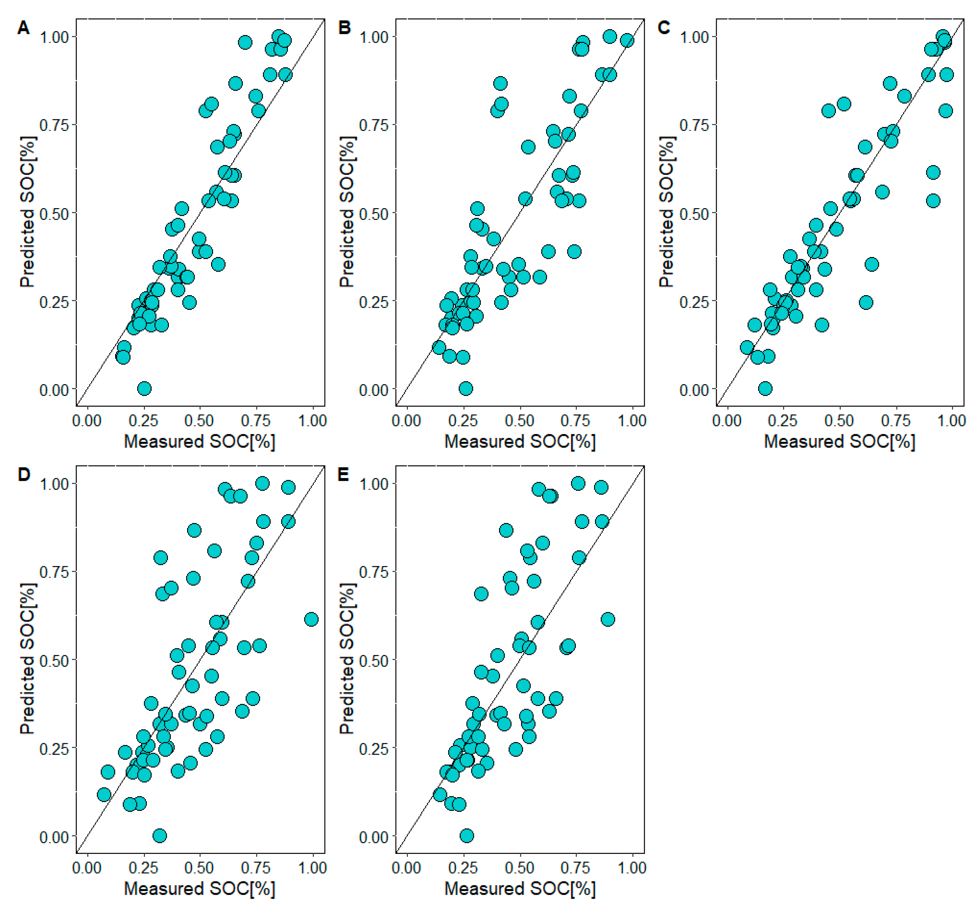
3.4. SOC Estimation Using Different MLAs

Prediction model accuracy was assessed using standard validation indices such as MAE, RMSE and R² by 10-fold cross-validation and repeated five times. The results for both the calibration and the validation datasets are listed in

Table 3. SOC calibration and validation results of the five machine learning models by 10-fold cross-validation.

Model	Calibration (n = 48)			Validation (n = 12)
	MAE	RMSE	R2	MAE	RMSE	R2
RF	0.15	0.17	0.64	0.17	0.20	0.68
Cubist	0.18	0.22	0.54	0.49	0.57	0.51
ANN	0.04	0.06	0.94	0.22	0.26	0.36
MLR	0.60	0.77	0.42	0.23	0.28	0.17
SVM	0.17	0.21	0.52	0.19	0.22	0.36

RF: random forest; ANN: artificial neural network; MLR: multiple linear regression; SVM: support vector machine.

. The model output was good using the calibration dataset (n = 48) except for MLR that gave an unacceptable prediction with calibration datasets (0 < R² < 0.50). In the calibration, the best performing model was ANN followed by RF, cubist, SVM and MLR with R² values of 0.94, 0.64, 0.54, 0.52 and 0.42, respectively. Using the validation dataset, the proposed MLA models showed their capabilities to predict SOC contents at an unsampled location in the southeastern region of Nigeria. The best performing model was RF (R² = 0.68) followed by the cubist model (R² = 0.51), SVM (R² = 0.36), ANN (R² = 0.36) and MLR (R² = 0.17). According to Li et al.’s [47] proposed model accuracy classification, RF and cubist models gave acceptable prediction as they fell within 0.50 < R² < 0.75, while ANN, MLR and SVM gave unacceptable prediction (0 < R² < 0.50) for SOC in flat terrain conditions. The R² value reported in the current study was higher than that of Wang et al. [20]. They achieved an R² mean value of 0.48 of the total spatial SOC variability using the RF algorithm in a flat terrain of semiarid pastures of eastern Australia. Using, MLR, ECEC was the most important variable with lower R² value when compared to Nath [63] who reported R² of 0.31 with curvature as the important variable.

The RF algorithm showed the lowest mean MAE value (0.17) of the five studied ML algorithms. The cubist algorithm had the highest error with mean RMSE values of 0.57 compared with other ML models; meanwhile, RF outperformed with the lowest mean RMSE value (0.20). Contrary to the report by Emadi et al. [15] who stated that ANN, RF and cubist models had a similar predictive ability to forecast SOC in the Mazandaran province of Iran, in this current study, only RF and cubist models showed similar predictive ability. In addition, the study also contradicts the report by Taghizadeh-Mehrjardi et al. [6] and Zhang et al. [45] that reported ANN as the best model. Concerning R², the low predictive ability of ANN has been reported by Mosleh et al. [10]. However, this model could be improved by the acquisition of large datasets and parameters in order to fit the model that yields good performance [64].

Figure 8 shows the scattered plots of RF, cubist, ANN, MLR and SVM predicted versus the measured SOC, respectively. In the figures, the central lines (1:1 line in black color) represented (predicted = measured). In Figure 8A reveals that RF scattered plots were more closed to the measured line than others. The plot further substantiated the MAE, RMSE, R² values obtained here, indicating RF as the best model predicting SOC at point scale for both calibration and test datasets using both environmental and soil nutrient indicators as variables.

Generally, Bou Kheir et al. [65] reported that SOC variation in the floodplain of Denmark is explained by both environmental variables, remote sensing data, and soil-related data. Wiesmeier et al. [66] reported that land use, soil types, and parent materials were the most critical variables controlling SOC distribution. Adhikari et al. [67] demonstrated the usefulness of environmental variables plus soil-related variables in explaining the SOC distribution down the soil depth in flat terrain. Besides the works mentioned above, this current study seems to contribute to the variables of choice in SOC prediction by including soil nutrient indicators (Ca_Mg, ECEC, BS, K_Ca) and these soil nutrient indicators are vital in crop growth and development. What happens in a flat terrain condition is that there is a slow rate of organic matter degradation and since soil organic matter has a large exchangeable site, basic cations (Ca²⁺, Mg²⁺, K⁺ and Na⁺) are absorbed into the soil solution [68,69,70]. On the other hand, environmental variables that are supposed to facilitate the process of soil organic matter decomposition are impeded because these activities are carried on a homogenous terrain. Thus, they make very little or no contribution to SOC prediction as exposed in this current paper.

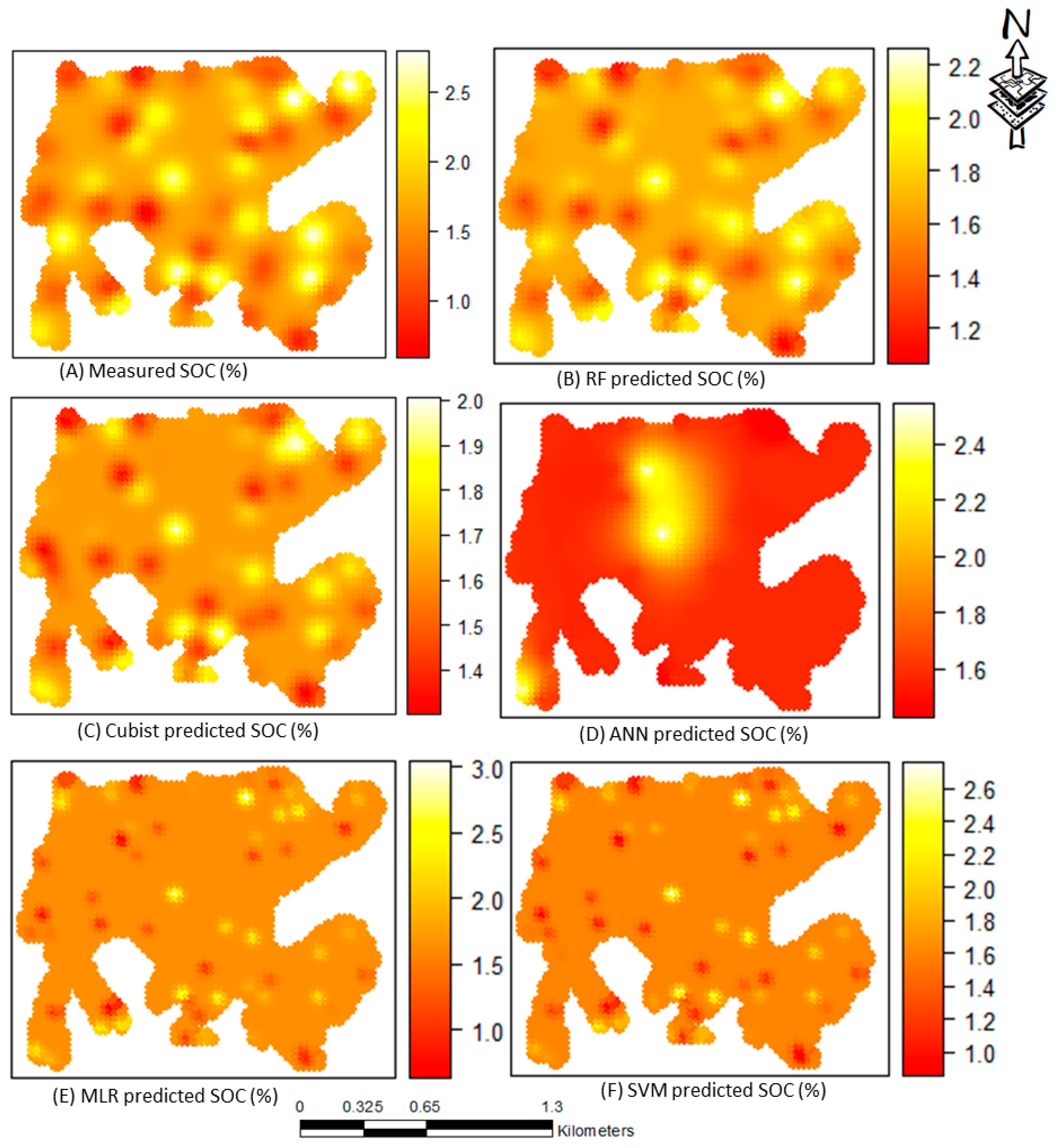
3.5. Digital Soil Mapping of SOC

The spatial result of digital SOC maps was produced with extracted cultivated land via the different models (RF, cubist, ANN, MLR and SVM) (Figure 9). RF and cubist models’ predicted SOC maps (Figure 8A) were relatively similar to the measured SOC map (Figure 9B) and showed substantial spatial variability of SOC. High predicted SOC values occurred in the center, northeastern, eastern and northwestern and southern parts of the research area, where the land was mainly covered by groundnut, pumpkin, litter falls as a result of dense vegetation cover. In addition, long-term application of organic manure could explain the high SOC contents in these parts of the research area used for cultivation. Similarly, the dominant low values were observed in all the parts of the maps were possible because of the loss of soil nutrients in the area through active cultivation without proper management procedures.

The maps generated by the MLR and SVM models are presented in Figure 9E,F, which highlight the high and low values in all the geographical positions of the maps. Compared with the RF, cubist, MLR and SVM models, the map of ANN more strongly manifested low SOC values in all the parts with high values at the center of the study area. Moreover, the map obtained by MLR resembled that of the SVM model (however, the map acquired by MLR ranged from 1.0 to 3.0% while SVM ranged from 1.0 to 2.6%).

4. Conclusions

In conclusion, among several predictors considered in this current study, environmental variables (b5, topographic wetness index and total catchment area), and soil nutrient indicators (Ca_Mg, ECEC, BS, K_Ca) had a significant influence on SOC distribution in the study area. They are valuable indicators in SOC prediction in flat homogenous topography. The RF model was the best model in the study. The resulting SOC map from RF prediction showed low SOC in the east and high SOC in the west direction of the site. The map suggests the gradual transportation and deposition of soil sediments. The study confirmed that SOC distribution could be digitally mapped through the five models as expected but more accurately with either RF or cubist models. Moreover, soil nutrient indicators, topographic wetness index and total catchment area were closely related to the SOC content in flat slope conditions.

From the study, soil nutrient program for SOC improvement could be implemented via RF and cubist models, incorporated into the digital soil mapping approach. However, RF showed to be a useful tool in prediction. The accuracy indicated that they act to reduce bias, and they can accommodate random inputs and random features to produce good results in classification—less so in regression. Cubist models generally give better results than those produced by simple techniques such as multivariate linear regression, while also being easier to understand than ANN.

Typically, low SOC levels require the application of organic manures, fallow cropping systems, organic fertilizer application and residual cropping to increase SOC levels. Through the application of MLAs in conjunction with digital soil mapping, the proper understanding of existing soil conditions may be gathered and thus allow precise soil management for sustainable crop production. This research sets a precedent for future digital soil mapping in other regions of Nigeria. Future studies should include other auxiliary predictors (e.g., soil physical and chemical properties, and lithological data) as well as cover a broader range of soil types to improve model performance.

References

1. Amalu, U.C.; Isong, I.A. Status and spatial variability of soil properties in relation to fertilizer placement for intercrops in an oil palm plantation in Calabar, Nigeria. Niger. J. Crop Sci. 2018, 5, 58–72. [Google Scholar]
2. Akpan, J.F.; Aki, E.E.; Isong, I.A. Comparative assessment of wetland and coastal plain soils in Calabar, Cross River State. Glob. J. Agric. Sci. 2017, 16, 17–30. [Google Scholar] [CrossRef] [Green Version]
3. Jenny, H. Factors of Soil Formation: A System of Quantitative Pedology, 1st ed.; McGraw-Hill Inc.: New York, NY, USA, 1941. [Google Scholar]
4. Chikezie, I.A.; Eswaran, H.; Asawalam, D.O.; Ano, A.O. Characterization of two benchmark soils of contrasting parent materials in Abia State, Southeastern Nigeria. Glob. J. Pure Appl. Sci. 2010, 16, 23–29. [Google Scholar] [CrossRef]
5. Amalu, U.C.; Isong, I.A. Land capability and soil suitability of some acid sand soil supporting oil palm (Elaeis guinensis Jacq) trees in Calabar, Nigeria. Niger. J. Soil Sci. 2015, 25, 92–109. [Google Scholar]
6. Taghizadeh-Mehrjardi, R.; Nabiollahi, K.; Kerry, R. Digital mapping of soil organic carbon at multiple depths using different data mining techniques in Baneh region, Iran. Geoderma 2016, 266, 98–110. [Google Scholar] [CrossRef]
7. Bian, Z.; Guo, X.; Wang, S.; Zhuang, Q.; Jin, X.; Wang, Q.; Jia, S. Applying statistical methods to map soil organic carbon of agricultural lands in northeastern coastal areas of China. Arch. Agron. Soil Sci. 2020, 66, 532–544. [Google Scholar] [CrossRef]
8. Chen, L.; Ren, C.; Li, L.; Wang, Y.; Zhang, B.; Wang, Z.; Li, L. A Comparative Assessment of Geostatistical, Machine Learning, and Hybrid Approaches for Mapping Topsoil Organic Carbon Content. ISPRS Int. J. Geo-Information 2019, 8, 174. [Google Scholar] [CrossRef] [Green Version]
9. Kingsley, J.; Lawani, S.O.; Esther, A.O.; Ndiye, K.M.; Sunday, O.J.; Penížek, V. Predictive Mapping of Soil Properties for Precision Agriculture Using Geographic Information System (GIS) Based Geostatistics Models. Mod. Appl. Sci. 2019, 13, 60. [Google Scholar] [CrossRef] [Green Version]
10. Mosleh, Z.; Salehi, M.; Jafari, A.; Esfandiarpour, I.; Mehnatkesh, A. The effectiveness of digital soil mapping to predict soil properties over low-relief areas. Environ. Monit. Assess. 2016, 188, 195. [Google Scholar] [CrossRef]
11. Zeraatpisheh, M.; Jafari, A.; Bodaghabadi, M.B.; Ayoubi, S.; Taghizadeh-Mehrjardi, R.; Toomanian, N.; Kerry, R.; Xu, M. Conventional and digital soil mapping in Iran: Past, present, and future. Catena 2020, 188, 104424. [Google Scholar] [CrossRef]
12. Akpan-Idiok, A.U.; Ukwang, E.E. Characterization and classification of coastal plain soils in Calabar, Nigeria. J. Agric. Biotechnol. Econ. 2012, 5, 19–33. [Google Scholar]
13. Baldock, J.A.; Wheeler, I.; McKenzie, N.; McBrateny, A. Soils and climate change: Potential impacts on carbon stocks and greenhouse gas emissions, and future research for Australianagriculture. Crop Pasture Sci. 2012, 63, 269–283. [Google Scholar] [CrossRef] [Green Version]
14. Minasny, B.; Setiawan, B.I.; Arif, C.; Saptomo, S.K.; Chadirin, Y. Digital mapping for cost effective and accurate prediction of the depth and carbon stocks in Indonesian peatlands. Geoderma 2016, 272, 20–31. [Google Scholar]
15. Emadi, M.; Taghizadeh-Mehrjardi, R.; Cherati, A.; Danesh, M.; Mosavi, A.; Scholten, T. Predicting and Mapping of Soil Organic Carbon Using Machine Learning Algorithms in Northern Iran. Remote Sens. 2020, 12, 2234. [Google Scholar] [CrossRef]
16. Wang, B.; Waters, C.; Orgill, S.; Cowie, A.; Clark, A.; Li, L.D.; Simpson, M.; McGowen, I.; Sides, T. Estimating soil organic carbon stocks using different modelling techniques in the semi-arid rangelands of eastern Australia. Ecol. Indic. 2018, 88, 425–438. [Google Scholar] [CrossRef]
17. Chen, D.; Chang, N.; Xiao, J.; Zhou, Q.; Wu, W. Mapping dynamics of soil organic matter in croplands with MODIS data and machine learning algorithms. Sci. Total Environ. 2019, 669, 844–855. [Google Scholar] [CrossRef]
18. Liu, S.; An, N.; Yang, J.; Dong, S.; Wang, C.; Yin, Y. Prediction of soil organic matter variability associated with different landuse types in mountainous landscape in southwestern Yunnan province, China. Catena 2015, 133, 137–144. [Google Scholar] [CrossRef]
19. Forkuor, G.; Hounkpatin, O.K.; Welp, G.; Thiel, M. High resolution mapping of soil properties using remote sensing variables in southwestern Burkina Faso: A comparison of machine learning and multiple linear regression models. PLoS ONE 2017, 12, e0170478. [Google Scholar] [CrossRef]
20. Wang, X.; Zhang, Y.; Atkinson, P.M.; Yao, H. Predicting soil organic carbon content in Spain by combining Landsat TM and ALOS PALSAR images. Int. J. Appl. Earth Obs. Geoinf. 2020, 92, 102182. [Google Scholar] [CrossRef]
21. Gehl, R.J.; Rice, C.W. Emerging technologies for in situ measurement of soil carbon. Clim. Chang. 2007, 80, 43–54. [Google Scholar] [CrossRef]
22. Al-Abbas, A.H.; Swain, P.H.; Baumgardner, M.F. Relating organic matter and clay content to the multi-spectral radiance of soils. Soil Sci. 1972, 114, 477–485. [Google Scholar] [CrossRef]
23. McMorrow, J.M.; Cutler, M.E.J.; Evans, M.G.; Al-Roichdi, A. Hyperspectral indices for characterizing upland peat composition. Int. J. Remote Sens. 2004, 25, 313–325. [Google Scholar] [CrossRef]
24. Viscarra Rossel, R.A.; Behrens, T. Using data mining to model and interpret soil diffuse reflectance spectra. Geoderma 2010, 158, 46–54. [Google Scholar] [CrossRef]
25. Fathololoumi, S.; Vaezi, A.R.; Alavipanah, S.K.; Ghorbani, A.; Saurette, D.; Biswas, A. Improved digital soil mapping with multitemporal remotely sensed satellite data fusion: A case study in Iran. Sci. Total. Environ. 2020, 721, 137703. [Google Scholar] [CrossRef]
26. Amalu, U.C.; Isong, I.A. Long-term impact of climate variables on agricultural lands in Calabar, Nigeria, I. Trend analysis of rainfall, temperature and relative humidity. Niger. J. Crop Sci. 2017, 4, 79–94. [Google Scholar]
27. Afu, S.M.; Isong, I.A.; Awaogu, C.E. Agricultural potentials of floodplain soils with contrasting parent material in Cross River State, Nigeria. Glob. J. Pure Appl. Sci. 2019, 25, 13–22. [Google Scholar] [CrossRef]
28. USDA NRCS. Soil Survey Staff. Keys to Soil Taxonomy, 12th ed.; United States Department of Agriculture, Natural Resources Conservation Service: Washington, DC, USA, 2014.
29. Akpan-Idiok, A.U.; Ogbaji, P.O. Characterization and Classification of Onwu River Floodplain Soils in Cross River State, Nigeria. Int. J. Agric. Res. 2013, 8, 107–122. [Google Scholar] [CrossRef]
30. Udo, E.J.; Ibia, T.O.; Ogunwale, J.A.; Ano, A.O.; Esu, I.E. Manual of Soil, Plant and Water Analyses; Sibon Books Limited: Lagos, Nigeria, 2009. [Google Scholar]
31. Roy, D.P.; Wulder, M.A.; Loveland, T.R.C.E.W.; Allen, R.G.; Anderson, M.C.; Helder, D.; Irons, J.R.; Johnson, D.M.; Kennedy, R.; Scambos, T.A.; et al. Landsat-8: Science and product vision for terrestrial global change research. Remote Sens. Environ. 2014, 145, 154–172. [Google Scholar] [CrossRef] [Green Version]
32. Breiman, L. Random forests. Mach. Learn. 2001, 45, 5–32. [Google Scholar] [CrossRef] [Green Version]
33. Heung, B.; Bulmer, C.E.; Schmidt, M.G. Predictive soil parent material mapping at a regional scale: A Random Forest approach. Geoderma 2014, 214, 141–154. [Google Scholar] [CrossRef]
34. Gislason, P.O.; Benediktsson, J.A.; Sveinsson, J.R. Random forests for land cover classification. Pattern Recogn. Lett. 2006, 27, 294–300. [Google Scholar] [CrossRef]
35. Díaz-Uriarte, R.; De Andres, S.A. Gene selection and classification of microarray data using random forest. BMC Bioinform. 2006, 7, 1–13. [Google Scholar] [CrossRef] [Green Version]
36. Zhou, J.; Li, E.; Wei, H.; Li, C.; Qiao, Q.; Armaghani, D.J. Random Forests and Cubist Algorithms for Predicting Shear Strengths of Rockfill Materials. Appl. Sci. 2019, 9, 1621. [Google Scholar] [CrossRef] [Green Version]
37. Rodríguez, J.D.; Perez, A.; Lozano, J.A. Sensitivity Analysis of k-Fold Cross Validation in Prediction Error Estimation. IEEE Trans. Pattern Anal. Mach. Intell. 2010, 32, 569–575. [Google Scholar] [CrossRef]
38. Quinlan, J.R. Learning with continuous classes. In Proceedings of the 5th Australian Joint Conference on Artificial Intelligence, Tasmania, Australia, 16–18 November 1992; pp. 343–348. [Google Scholar]
39. Kuhn, M.; Johnson, K. Applied Predictive Modeling; Springer: Berlin, Germany, 2013; Volume 26. [Google Scholar]
40. Wang, Y.W.I. Inducing Model Trees for Continuous Classes. In Proceedings of the 9th European Conference on Machine Learning; Springer: Berlin/Heidelberg, Germany, 1997; pp. 128–137. [Google Scholar]
41. Behrens, T.; Forster, H.; Scholten, T.; Steinrücken, U.; Spies, E.D.; Goldschmitt, M. Digital soil mapping using artificialneural networks. J. Plant Nutr. Soil Sci. 2005, 168, 21–33. [Google Scholar] [CrossRef]
42. Vapnik, V. The Nature of Statistical Learning Theory; Springer: New York, NY, USA, 1995. [Google Scholar]
43. Cherkassky, V.; Mulier, F. Learning from Data: Concept, Theory and Methods; John Wiley and Sons: New York, NY, USA, 1998. [Google Scholar]
44. Siewert, M.B. High-resolution digital mapping of soil organic carbon in permafrost terrain using machine learning: A case study in a sub-Arctic peatland environment. Biogeosciences 2018, 15, 1663–1682. [Google Scholar] [CrossRef] [Green Version]
45. Zhang, Y.; Sui, B.; Shen, H.; Ouyang, L. Mapping stocks of soil total nitrogen using remote sensing data: A comparison of random forest models with different predictors. Comput. Electron. Agric. 2019, 160, 23–30. [Google Scholar] [CrossRef]
46. R Core Team. R: A Language and Environment for Statistical Computing; R Foundation for Statistical Computing: Vienna, Austria, 2019; Available online: https://www.r-project.org/ (accessed on 13 May 2020).
47. Li, L.; Lu, J.; Wang, S.; Ma, Y.; Wei, Q.; Li, X.; Cong, R.; Ren, T. Methods for estimating leaf nitrogen concentration of winter oilseed rape (Brassica napus L.) using in situ leaf spectroscopy. Ind. Crop. Prod. 2016, 91, 194–204. [Google Scholar] [CrossRef]
48. Wilding, L.P.; Drees, L.R. Spatial variability and pedology. In Pedogenesis and Soil Taxonomy: Concepts and Interactions; Wilding, L.P., Smeck, N.E., Hall, G.F., Eds.; Elsevier: New York, NY, USA, 1983; pp. 83–116. [Google Scholar]
49. Denton, O.; Modupe, A.; Ojo, V.O.A.; Adeoyolanu, A.O.; Are, O.D.; Adelana, K.S.; Oyedele, A.O.; Adetayo, A.O.; Oke, A.O. Assessment of spatial variability and mapping of soil properties for sustainable agricultural production using geographic information system techniques. Cogent Food Agric. 2017, 3, 1–12. [Google Scholar] [CrossRef]
50. Reza, S.K.; Nayak, D.C.; Chattopadhyay, T.; Mukhopadhyay, S.; Singh, S.K.; Srinivasan, R. Spatial distribution of soil physical properties of alluvial soils: A geostatistical approach. Arch. Agron. Soil Sci. 2016, 62, 972–981. [Google Scholar] [CrossRef]
51. Landon, J.R. Booker Tropical Soil Manual: A Handbook for Soil Survey and Agricultural Land Evaluation in the Tropics and Subtropics; Longman: New York, NY, USA, 1991. [Google Scholar]
52. Bednářa, M.; Šarapatkaa, B. Relationships between physical–geographical factors and soil degradation on agricultural land. Environ. Res. 2018, 164, 660–668. [Google Scholar] [CrossRef]
53. Gelaw, A.M.; Singh, B.R.; Lal, R. Organic carbon and nitrogen associated with soil aggregates and particle sizes under different land uses in Tigray, Northern Ethiopia. Land Degrad. Dev. 2013, 26, 690–700. [Google Scholar] [CrossRef]
54. Anikwe, M.A.N. Carbon storage in soils of southeastern Nigeria under different management practices. Carbon Balance Manag. 2010, 5, 5. [Google Scholar] [CrossRef] [Green Version]
55. Six, J.; Feller, C.; Denef, K.; Ogle, S.M.; Sa, J.C.M.; Albrecht, A. Soil organic matter, biota and aggregation in temperate and tropical soils- Effect of no-tillage. Agronomie 2002, 22, 755–775. [Google Scholar] [CrossRef] [Green Version]
56. Lal, R. Soil Carbon sequestration impacts on global climate change and food security. Science 2004, 30, 1623–1627. [Google Scholar] [CrossRef] [Green Version]
57. Purwanto, B.H.; Alam, S. Impact of intensive agricultural management on carbon and nitrogen dynamics in the humid tropics. Soil Sci. Plant Nutr. 2020, 66, 50–59. [Google Scholar] [CrossRef]
58. Florinsky, I.V.; McMahon, S.; Burton, D.L. Topographic control of soil microbial activity: A case study of denitrifiers. Geoderma 2004, 119, 33–53. [Google Scholar] [CrossRef]
59. Akpan-Idiok, A.U.; Ogbaji, P.O.; Antigha, N.R.B. Infiltration, degradation rate and vulnerability potential of Onwu River floodplain soils in Cross River State, Nigeria. J. Agric. Biotechnol. Ecol. 2012, 5, 62–74. [Google Scholar]
60. Solly, E.F.; Weber, V.; Zimmermann, S.; Walthert, L.; Hagedorn, F.; Schmidt, M.W.I. A Critical Evaluation of the Relationship between the Effective Cation Exchange Capacity and Soil Organic Carbon Content in Swiss Forest Soils. Front. For. Glob. Chang. 2020, 3, 98. [Google Scholar] [CrossRef]
61. Song, Y.Q.; Yang, L.A.; Li, B.; Hu, Y.M.; Wang, A.L.; Zhou, W.; Cui, X.S.; Liu, Y.L.; Song, Y.Q.; Yang, L.A.; et al. Spatial prediction of soil organic matter using a hybrid geostatistical model of an extreme learning machine and ordinary kriging. Sustainability 2017, 9, 754. [Google Scholar] [CrossRef] [Green Version]
62. Li, X.; McCarty, G.W.; Du, L.; Lee, S. Use of Topographic Models for Mapping Soil Properties and Processes. Soil Syst. 2020, 4, 32. [Google Scholar] [CrossRef]
63. Nath, D.A. Soil Landscape Modeling in the Northwest Iowa Plains Region of O’Brien County, Iowa. Master’s Thesis, Iowa State University, Ames, IA, USA, 2006. [Google Scholar]
64. Padarian, J.; Minasny, B.; McBratney, A.B. Using deep learning for digital soil mapping. Soil 2019, 5, 79–89. [Google Scholar] [CrossRef] [Green Version]
65. Bou Kheir, R.; Greve, M.H.; Bøcher, P.K.; Greve, M.B.; Larsen, R.; McCloy, K. Predictive mapping of soil organic carbon in wet cultivated lands using classification-tree based models: The case study of Denmark. J. Environ. Manag. 2010, 91, 1150–1160. [Google Scholar] [CrossRef]
66. Wiesmeier, M.; Barthold, F.; Blank, B.; Kögel-Knabner, I. Digital mapping of soil organic matter stocks using Random Forest modeling in a semi-arid steppe ecosystem. Plant. Soil 2011, 340, 7–24. [Google Scholar] [CrossRef]
67. Adhikari, K.; Hartemink, A.E.; Minasny, B.; Kheir, R.B.; Greve, M.B.; Greve, M.H. Digital mapping of soil organic carbon contents and stocks in Denmark. PLoS ONE 2014, 9, e105519. [Google Scholar] [CrossRef]
68. Andersson, S.; Nilsson, I.; Valeur, I. Influence of dolomiticlime on DOC and DON leaching in a forest soil. Biogeo-Chemistry 1999, 47, 295–315. [Google Scholar] [CrossRef]
69. Chan, K.Y.; Heenan, D.P. Lime-induced loss of soil organiccarbon and effect on aggregate stability. Soil Sci. Soc. Am. J. 1999, 63, 1841–1844. [Google Scholar] [CrossRef]
70. Thirukkumaran, C.M.; Morrison, I.K. Impact of simulated acid rain on microbial respiration, biomass, and metabolic quotient in a mature sugar maple (Acer saccharum) forest floor. Can. J. For. Res. 1996, 26, 1446–1453. [Google Scholar] [CrossRef]
Figure 1. Geographical position of the study area in Cross River State.
Land 09 00487 g001
Figure 2. Correlation matrix between SOC (%) and environmental variables and soil nutrient indicators.
Land 09 00487 g002
Figure 3. Relative importance variable for SOC using random forest (RF) model.
Land 09 00487 g003
Figure 4. Relative importance variable for SOC using cubist model.
Land 09 00487 g004
Figure 5. Relative importance variable for SOC using an artificial neural network model.
Land 09 00487 g005
Figure 6. Relative importance variable for SOC using multiple linear regression (MLR).
Land 09 00487 g006
Figure 7. Relative importance variable for SOC using support vector machine (SVM).
Land 09 00487 g007
Figure 8. Measured vs. predicted values of soil organic carbon using five machine learning algorithms:(A) RF, (B) cubist, (C) ANN, (D) MLR and (E) SVM. (RF: random forest; cubist: regression tree; ANN: artificial neural networks; MLR: Multiple linear regression; SVM: support vector machine).
Land 09 00487 g008
Figure 9. Prediction maps for soil organic carbon.
Land 09 00487 g009