Methodology and Results of Staged UAS Photogrammetric Rockslide Monitoring in the Alpine Terrain in High Tatras, Slovakia, after the Hydrological Event in 2022

Abstract

There are numerous talus cones that have formed by long-term geological processes and sudden hydrological events in the Small Cold Valley (High Tatras National Park in Slovakia). Frequent hiking trails lead here; therefore, their safeness needs to be monitored due to recent rock avalanches and landslides. A complex methodology for monitoring changes in talus cones was developed to determine the extent, pace, nature, and origin of the morphological changes in the land in this complex high-mountain terrain. Non-contact UAS photogrammetry with SfM-MVS processing was applied as a quick, reliable, and environment-friendly data acquisition method. For proper georeferencing, a network of GCPs and stabilized surveying points were established by terrestrial geodetic surveying. Together with an evaluation of the methodology, the results comparing the actual state of a talus cone in 2018 and 2022 (after the significant hydrological event) are presented. Comparing and analyzing spatial models represented by point clouds, with an accuracy of centimeter level, was obtained. The detected morphological changes reached values in meters. A differential model expresses the distribution of the morphological changes. In conclusion, geodetic and geological knowledge is synthesized to evaluate the phenomena occurring in this territory.

1. Introduction

Landslide monitoring in alpine environments is important in landslide analysis, cause determination, and prediction. Steep rock valleys and slopes prone to erosion and landslides pose a safety risk, especially for mountain visitors—these are often the most frequented hiking trails leading to alpine huts in the High Tatras during the summer season [1,2]. An example of such a locality is a rockslide in the Small Cold Valley in the High Tatras at an altitude of 1700 m. It is part of the Tatra National Park with the highest level of protection (Level 5), which is completely determined by nature and its phenomena. Practically, this means that geohazards cannot be and are not structurally or technically sanitized in any way. Therefore, regular spatial and temporal geodetic monitoring, geological and hydrological analyses, and the monitoring of meteorological aspects of the occurrence of abrupt events are required to maintain the safety of such places.

Different methods can be used for landslide monitoring, which can be divided according to the disciplines (geotechnics, hydrology, remote sensing, etc.) for which the results are used, as described clearly in [3]. The basic methods fall under the category of geotechnical ones; they estimate the mass transfer speed, the depth of the landslide area, and the movement direction. Geotechnical observations are made using inclinometers, extensometers, dilatometers, and other similar devices. These instruments and techniques measure with high accuracy (up to sub-millimeters), but the intended changes are only relative and at a given point. Therefore, geotechnical methods are often combined with data containing absolute displacement determinations [4], which can be obtained by geodetic monitoring. Geodetic and photogrammetric measurement methods are frequently used, from which it is possible to interpret the displacements and deformations of the area of interest over time [5]. When monitoring landslides and deformations affecting technical or construction objects, such as slopes near highways, it is necessary to stabilize the network of reference and observed points [6]. The study [7] also mentions relevant methods based on remote sensing (multispectral satellite imagery, satellite radar interferometry, and Doppler radar). However, there may be a disadvantage in the frequency of the passage of the relevant satellites over a given location. A very effective method is terrestrial InSAR [8], which is commonly placed on a linear base and images the opposite slope in a time series, as reported in [9] and [10]. However, this system cannot always be used; there must be favorable conditions for this, in particular, the entire landslide area to be monitored must be visible from a ground position. This is practically impossible to guarantee in the case of alpine landslides. The instrument itself is also very expensive.

As some studies have shown, combining different methods for complex landslide monitoring is advantageous. In [11], a combination of multitemporal InSAR and inclinometric boreholes, and in [3], a combination of inclinometers, GNSS receivers, multitemporal InSAR, and UAV photogrammetry were used. The determination of spatial changes in landslide areas using classical geodetic or remote sensing methods was addressed in [12]. UAS photogrammetry and laser scanning methods are often used for the documentation and monitoring of landslides, rockfalls, and geohazards at small scales [13].

Geodetic monitoring is realized by surveying methods from which spatial changes in the area of interest over time can be interpreted [5]. Before geodetic monitoring, it is necessary to stabilize the network of reference points in stable areas and the network of observed points that must cover the entire area of the slope or landslide [6]. For example, global navigation satellite systems (GNSS) and trigonometric methods of measurement using total stations (TS) can be used as surveying methods [14]. Their deployment can be in periodic stages or permanent, which is often automated [15,16]. However, in the case of high-altitude alpine environments, these options are limited by technical or regulatory constraints.

Furthermore, these surveying methods are performed on a limited number of specific points; therefore, they do not provide a complete record of the measured object’s surface. Consequently, they are unsuitable for analyzing morphological changes in irregular formations such as landslides [17]. Especially in analyzing rock failures and deformations of planar rock formations—in our case, a debris cone—it is particularly appropriate to use non-contact, non-selective methods of mass spatial data collection [18]. The result of such measurements is a primary point cloud that allows for the creation of spatial 3D models [19].

The first method used in the current study was terrestrial laser scanning (TLS) [20], which has the advantages of high accuracy in determining the positions of the observed points and a high density of the resulting point cloud [21]. However, the disadvantages, especially in rugged areas, are a higher measurement time, acquisition cost, and especially occlusions [22], resulting in the incompletion of the digital surface model (DSM). Minimizing occlusions can be achieved by densifying the scanner stand positions, but their complete elimination is impossible. This shortcoming of the TLS method could be complemented by using lidar technologies based on simultaneous localization and mapping (SLAM) algorithms [23].

The airborne laser scanning (ALS) method can also be used. The disadvantages, especially at higher flight heights above the ground (AGL), are a lower density of the point cloud, poorer vertical accuracy, and point distortion due to the size of the laser footprint. Comparisons of the results of ALS-based measurements with other methods are shown in [24,25,26]. The shortcomings of ALS can be largely eliminated by using unmanned aerial system (UAS)-borne lidar technology [27,28].

However, the most widespread method for obtaining a digital terrain model in recent years has been the modern structure-from-motion (SfM) photogrammetry method. UAS are now effectively used as carriers of photogrammetric cameras [29]. This method is very advantageous regarding economic and time efficiency. As a result, a high-density point cloud can be obtained. As a disadvantage, adequate illumination of the measured object is needed [30].

The combination of lidar and photogrammetry, whose simultaneous processing Is enabled by some software, is also suitable. For example, in [31], the authors combined mobile laser scanning and UAS photogrammetry to map a riverbed.

Direct or indirect georeferencing is also an essential factor in the methodology of developing the use of these methods [32]. Ground control points (GCPs), which can be naturally or artificially signaled, are used to determine the scale of lidar and photogrammetric models and often for their indirect georeferencing. The CORS/RTK determination of the position of the camera projection center directly during the flight seems to be an ideal approach, which guarantees high accuracy and the possibility of reducing the number of GCPs [33,34]. The quality of models with different georeferencing approaches has been addressed, e.g., by the authors in [35,36].

When processing the results of measurements by non-selective methods, the classification of point clouds is needed. This is the filtering of natural and anthropogenic features that are unnecessary or undesired for creating a spatial model of the object of interest, as they would distort the proper shape of an object. Most often, these are vegetation, buildings, persons, etc. Analytical procedures based on object geometry were used in the paper [37]. The goal is to automate the feature of the interest extraction process mainly to speed it up [38,39]. For the filtering of vegetation from point clouds, methods based on the analysis of vegetation indices can also be used [40]. The analysis of point clouds and the creation of 3D models have been the subject of many works in both natural [41] and artificial environments [42].

The documentation of landslides is addressed in [43,44], as is the monitoring of landslides, rockfalls, and geohazards in [45,46,47]. In [43], the authors monitored an active landslide long-term using the GNSS method at several observed points. They also applied UAS-SfM photogrammetry to analyze the landslide surface in several stages. A comparison was made based on the cross-sections and differential models. C2C differences were detected in the range of up to 4m, with values AGL 110 m and GSD 4 cm. In [44], an active landslide with an area of 1250 m² was investigated using multitemporal UAS surveys. The measurement stages were also realized before and after intense rainfall. The differences between the stages and the volume of the moved material were determined from the DTM. The authors also dealt with the data classification, as it was an area covered with vegetation. The authors in [45] dealt with UAS monitoring and stability research of rock walls. They used a combination of UAS- and SfM-based ground photogrammetry. The UAS data were used for a model of the whole area, while the ground-based photogrammetry was used to reconstruct details. The structural–geological parameters were also determined from the obtained data. The evaluation results of displacement and deformations of the ground induced by a landslide were analyzed from the results of airborne laser scanning and UAS-borne laser scanning [46]. A model with a density of 8 points/m² was obtained using ALS. During the UAS-borne laser scanning, they obtained 500 points/m² with a positional accuracy of 4 cm. They evaluated changes with an average size of 13.2 cm. The authors in [47] dealt with the documentation and prediction of the marine erosion of the rocky coast based on point cloud analysis and orthophoto maps. They used a UAS Phantom 4 Pro with a dedicated camera. They shot from a height of 120 m with a GSD of 3.26 cm. For georeferencing, they used the GCPs determined by RTK GNSS with an accuracy of 2 cm in position and 5 cm in height.

In our previous research [48,49], we have focused on the application of several methods of spatial data collection (the evaluation of their quality, efficiency, and accuracy). Based on the experience gained, and due to the high importance of the geodetic monitoring of rock slides in difficult alpine terrain, the following are presented in the present paper: (i) the methodology of the epoch measurements by SfM UAS photogrammetry, (ii) the processing of datasets, and (iii) an example of the evaluation of the epoch measurements in terms of determining the change in the shape of the landslide surface and the determination of the volume of displaced material caused by the impact of extreme precipitation in the Small Cold Valley in 2022.

2. Materials and Methods

2.1. Methodology of Long-Term Photogrammetric UAS Landslide Monitoring

The monitoring preparation started with a field reconnaissance. It was necessary to select stable and visible locations to install the geodetic network points that would guarantee comparable results in the epoch measurement [49]. The network points can be stabilized permanently directly to the rock mass through drilled metal spikes or a reflective foil. These points are then, during surveying, signaled by reflective prisms on the metal mandrels. The staged evaluation of the results requires the determination of geodetic network points significantly more accurately than the method used for mass data collection (in this case, UAV photogrammetry), so it was advisable to carry out the survey using a total station. Ideally, the measured quantities must be balanced according to the least squares method, and the result is then the adjusted coordinates of the geodetic network. For the correct georeferencing of the geodetic network to the reference system, it is advantageous to use the GNSS (Global Navigation Satellite System) method, but this is not entirely necessary for staged measurements. For these purposes, measurement with one receiver connected to a network of permanent reference stations is sufficient [45]. If there is no internet connection available for an online solution, it is possible to perform a short observation with a fast static method and obtain the coordinates by post-processing using data from the nearest permanent stations usually available from the service provider’s repository [45]. The advantage of georeferencing is the possible use of a UAS with GNSS real-time kinematic (RTK) technology, allowing for more straightforward calculation processing.

Preparation for the standard stage started again with a terrain reconnaissance, during which it was necessary to identify locations for ground control points (GCPs) and checkpoints (CPs). These needed to be visible from the UAS and, at the same time, targetable by a total station. GCPs should be placed around the perimeter of the monitored area with several points in the middle. When using a UAS equipped with a GNSS RTK/PPK function, it is necessary to implement at least a few GCPs to correct the elevation component, as reported in [36]. Only a few CPs spaced evenly in a given area are sufficient. Stabilization and signalization of these points are realized temporarily using black and white photogrammetric targets, or in many cases, it is sufficient to mark the GCPs with a colored spray. Both GCPs and CPs should be of such a size that the positions of the points (centers of the targets or colored spray marks) can be well identified on the images, i.e., the size of the point on the image should be at least 5 pixels or larger (i.e., in reality, 5× GSD). A total station should be used to determine their position to eliminate systematic differences between the stages [45]. Before measurement, it is advisable to first use the total station to perform a geodetic network check, which is nowadays possible with computational algorithms implemented directly in the total station (e.g., using the free station calculation task).

The UAS flight design can be divided into several stages. First, it is necessary to consider the resulting desired point cloud accuracy, which is related to the choice of UAS and camera parameters. For the UAS, there is a choice between equipment with or without GNSS RTK/PPK receiver and regarding flight time. The choice of camera is, in turn, crucial for the actual data (image) collection. Important camera parameters include the sensor resolution and the lens’s focal length. These parameters and the flight height AGL determine the ground sample distance (GSD, i.e., the pixel size of surveyed object in reality). This value determines how detailed terrain can be captured and also enters as a control mechanism into the computational process regarding accuracy.

In the case of mountainous terrain, the monitored area is almost always at some slope. Therefore, it is advisable to consider the flight parameters. If the flight planning software allows it, the ideal flight choice is to fly the UAV at a given distance from the terrain and follow the terrain at a constant AGL. If this option is not available, the monitored area can be divided into sub-parts. However, there will always be a slight discrepancy in the GSD value. This issue can be resolved by lowering the flight height so that the path at the highest point from the ground meets the predetermined GSD from the flight altitude, sensor parameters, and accuracy requirements. The area can also be divided into sub-areas within which this requirement is met.

The flight mission can be performed automatically or manually. When creating an automatic flight mission, choosing to fly in one direction only (grid) or in two perpendicular directions (double grid) is possible. Regarding photogrammetric practice, using a double-grid flight mission is advisable [34]. This increases the number of images and minimizes uncaptured locations (occlusions). Flight planning is also related to the setting of longitudinal and lateral overlays on the images, which are essential for the calculation. In the case of a single flight path, it is advisable to specify overlays in both directions up to 90 percent. It may happen that the UAS in an automated flight mission will not maintain the set path due to weather conditions. Images with insufficient overlays will then not be evaluated. Of course, it is also possible to perform the flight manually, but from experience, we recommend choosing an automatic mission, as in mountainous terrain (in the case of a rock field, everything is very similar in the images). In our opinion, the operator is not able to ensure the correct overlays. For better stability of the computational model, some UAS can also take oblique images automatically, which we definitely recommend [34,36]. In the case of sloping terrain, it is advisable to consider setting the direction of imaging perpendicular to the terrain.

For double-grid flights, an overlap of approximately 60 to 80 percent is commonly used. In principle, the use of a higher overlap does not harm the results, it just increases the UAS’s length of trajectory, which is directly related to the expected flight time and battery life. A strong wind also significantly reduces flight time. Finally, knowing when the UAS can be used more powerfully and efficiently is necessary.

The UAS flight should be conducted during the daytime when light and shadows are not changing, preferably when it is slightly overcast. Changes in light and shadows can cause a problem in the subsequent calculation.

The calculation is carried out in specialized software and should always be checked using the achieved deviations on the GCPs, the value of which should be around 1 to 2 times the GSD. These values may reveal possible errors in the calculation of the image orientations. When using a drone with GNSS RTK/PPK, these possible errors are partially reduced, as the camera positions are accurately determined during flight. It is also necessary to check the evaluation of CPs that could theoretically indicate a twist in the photogrammetric model. The deviations in the CPs, based on the authors’ experience, can range from about 1 to 3 times the GSD. The result of the SfM-MVS reconstruction is a point cloud of the surveyed area, from which, before further analyses, it is usually necessary to clean up the vegetation points by different classification methods, e.g., as in [38].

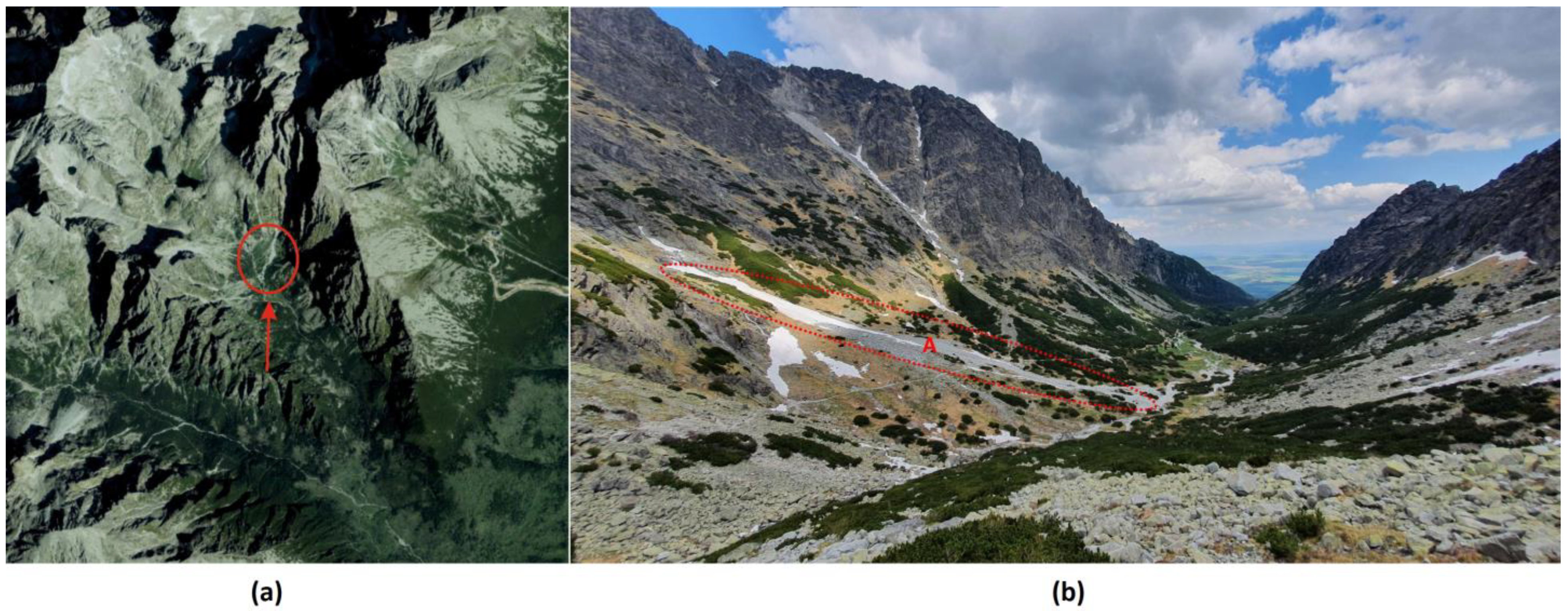
2.2. The Test Site

The monitored area was a talus cone in the Small Cold Valley. This is a terraced valley located in the Slovak part of the High Tatras (see Figure 1). The length of the valley is approximately 4.5 km. It is bounded in the east by the Lomnický saddle and in the west by the Prostredný ridge, which separates it from the Large Cold Valley. At its end is the Basin of the Five Spišské ponds, bordered by the massif of the Ice Peak (2627 m). The Small Cold stream crosses the valley. The Small Cold Valley has typical alpine vegetation. Pine trees, either in the form of slash pine or limber pine, are the most abundant species. Deciduous trees are also present, mainly in the form of scrub. Alpine meadows are characteristic at higher altitudes. Typical representatives of the local fauna are the mountain chamois and the mountain marmot. The Small Cold Valley is one of the most visited valleys in the High Tatras. In addition to hiking, mountaineering is also an attraction here. Several geomorphological formations of debris flow prevail throughout the area of interest. Flows are increasingly active due to the enormous rainfall over the last ten years. These can be potentially included in geohazards, as they are located in the tourist-frequented valleys of the High Tatras (often crossed by frequented high mountain hiking routes). The area shown in Figure 1 was selected as the object of our research.

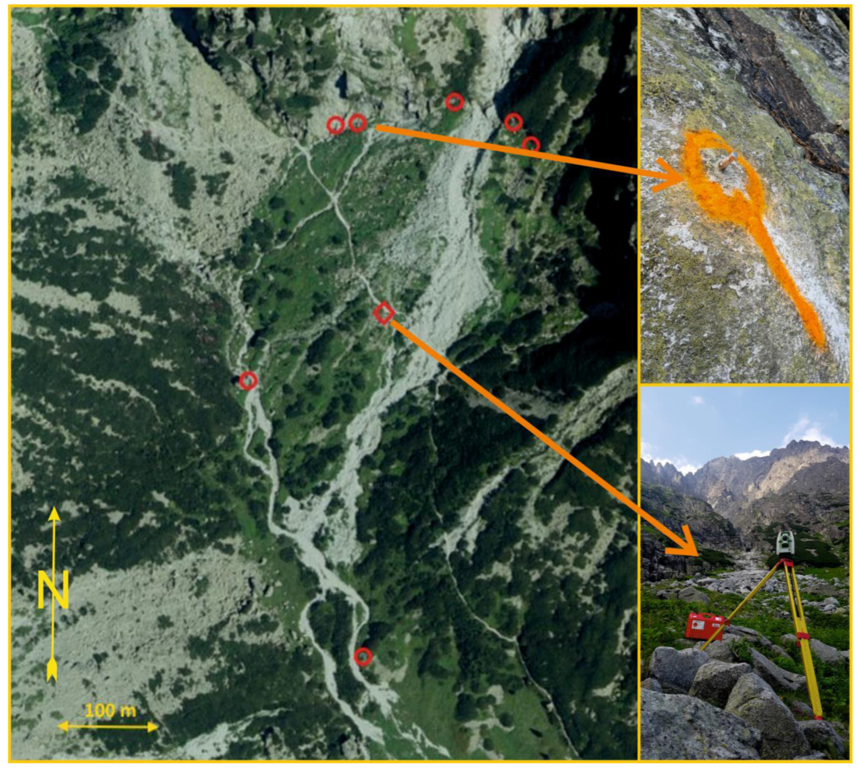
2.3. Reference Geodetic Network, Stabilization of Reference Points

For research purposes, it was necessary to build a precise geodetic network. The geodetic network was stabilized by four stainless steel pins fixed into the rock with Fischer chemical mortar. In addition, three reflective targets (reflective foils) were glued with an adhesive (Pattex Chemopren Universal) on suitable flat rock surfaces and large stone blocks where immutability over time could be assumed.

A scheme of the location of the reference network points is shown in Figure 2. The points were stabilized in advance of the actual measurements to avoid changes in shape between stages. The coordinates of the points were determined by a total station from a single position with an accuracy better than or equal to 0.01 m. Georeferencing was determined using three additional points determined by a GNSS RTK receiver with an online connection to the SKPOS real-time positioning service. The observation time at one point was 5 min, and the rod was placed in a stand. The estimated accuracy (according to the service provider, https://skpos.gku.sk/, accessed on 23 March 2023) was 0.02 m in position and 0.04 m in height. Comparable accuracy of the GNSS to the total station measurements could not be expected, but the overall location of the reference network was not necessary for determining the changes, as the same initial geodetic network was used at each stage.

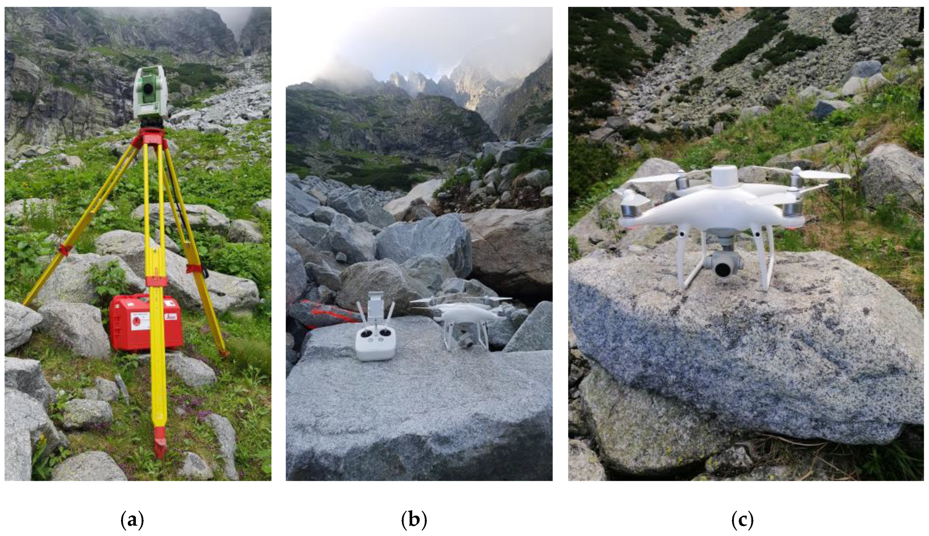
2.4. Instruments and Equipment

For the geodetic measurements, a Leica TS02 total station was used (horizontal measurement accuracy of 7”, length measurement accuracy on a reflecting prism or reflective foil of 1.5 mm + 2.0 ppm, see Figure 3a). For image acquisition, a DJI Phantom 4 Pro UAS was used in the first epoch (June 2018, see Figure 3b)), whose internal camera was equipped with a 20Mpix CMOS sensor (5472 × 3648 pixels). The UAS weighed 1.4 kg and had a maximum flight time of 30 min. The images in the second epoch (June 2022) were acquired by DJI Phantom 4 RTK UAS equipped with a camera with identical parameters but supplemented by an onboard GNSS RTK receiver, enabling higher (centimeter) accuracy of the camera coordinates (see Figure 3c).

Pix4D Capture software was used for the flight planning in the first epoch, and DJI GS RTK in the second. The DJI GS RTK field application allows for flight planning where the flight height can be constant according to the shape or slope of the terrain, i.e., the UAV follows the terrain at the same AGL height.

2.5. Field Measurements

The experimental measurements consisted of the following consecutive activities:

• The determination of the position and orientation of the total station at the measurement site (see Figure 2, marked with a rhombus);
• The deployment and signalization of GCPs for photogrammetric imaging along the perimeter of the monitored area. Solving the points inside was unnecessary regarding its shape (the site is narrow and long);
• The measurement of the position and height of the GCPs by the total station;
• An automatic image flight was performed by entering the route into the control software.

The accuracy of the GCP position determination was assumed to be 0.005 mm or better in both stages (valid for each coordinate, corresponding to the accuracy of the total station measurement).

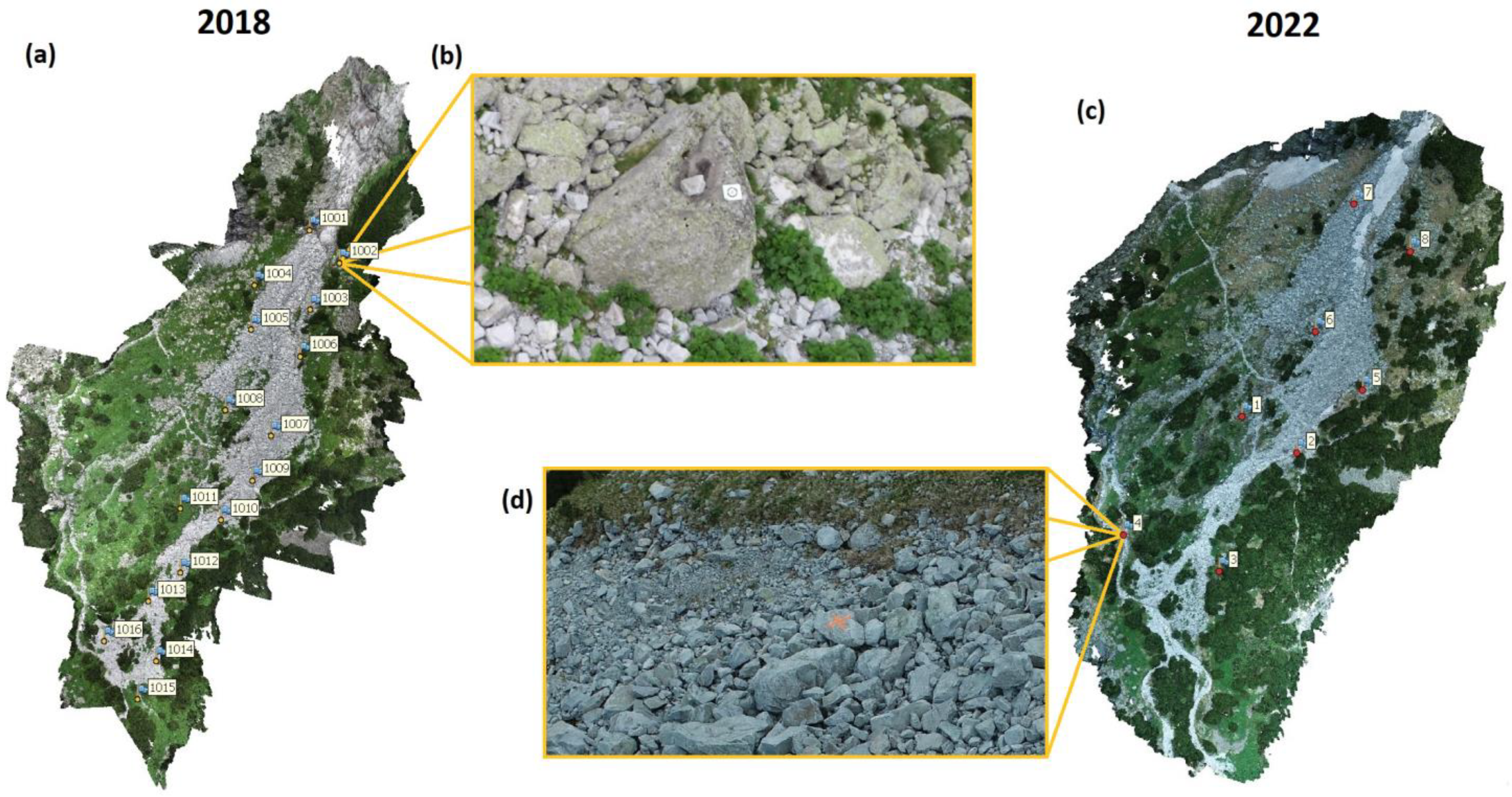
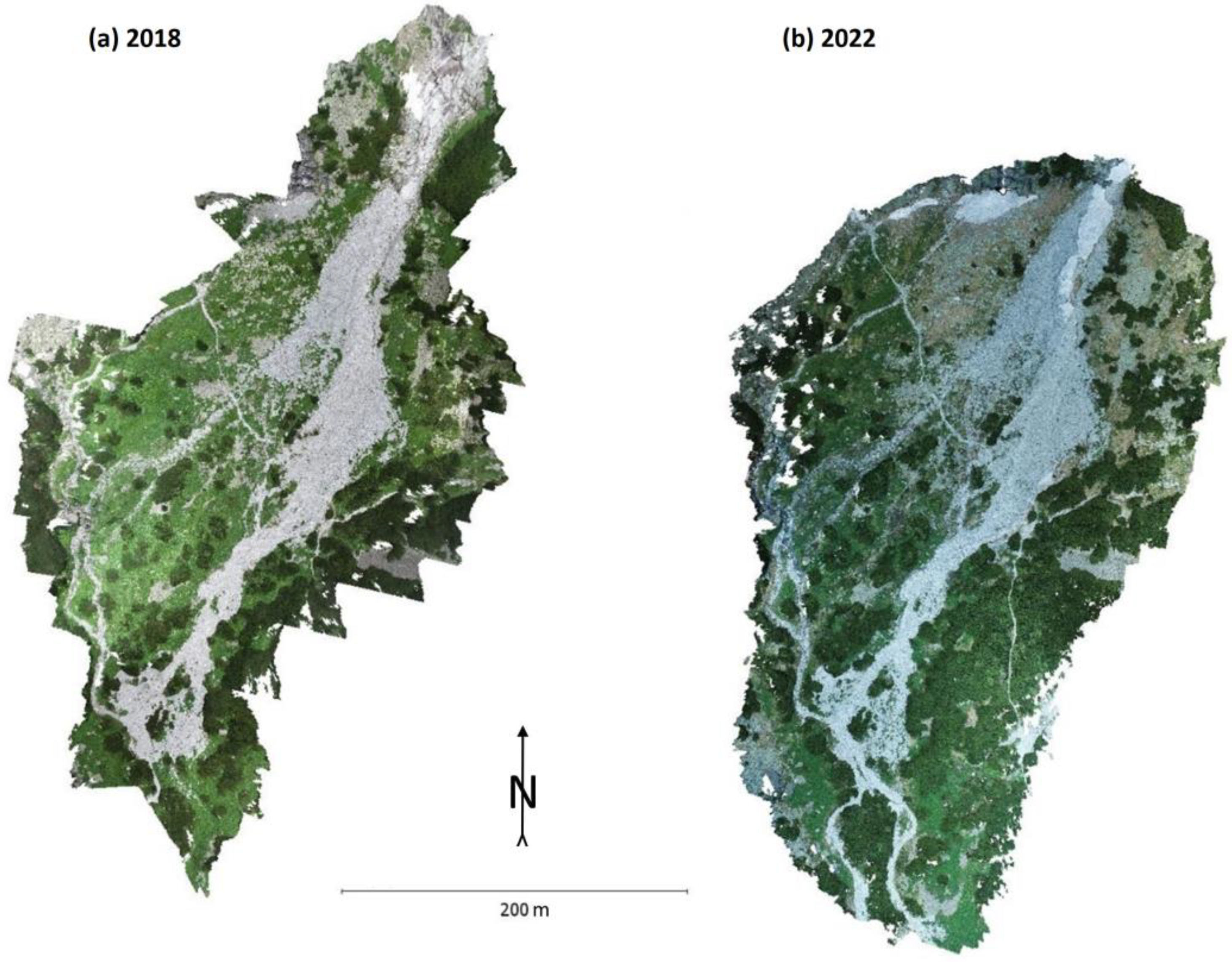
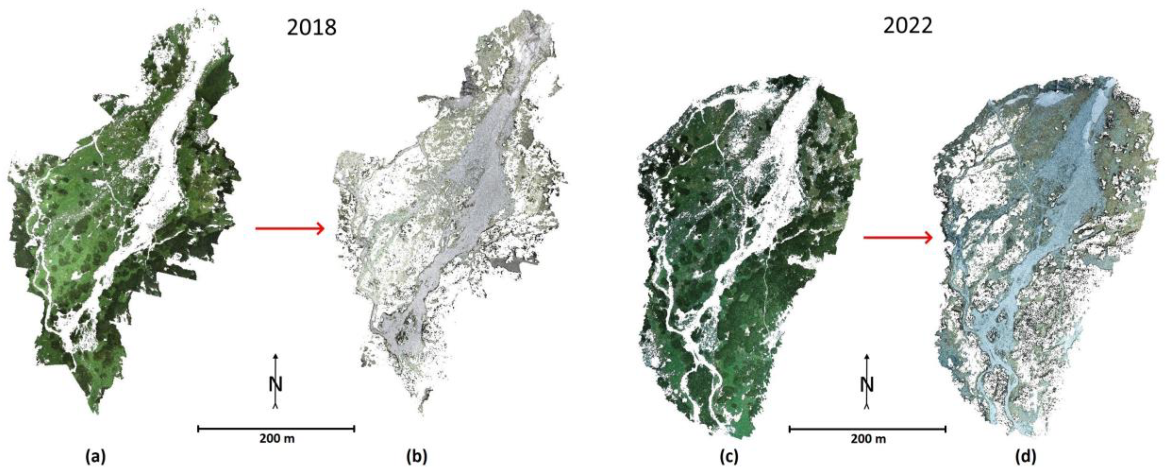
In the case of epoch 2018, regarding the significant slope of the terrain in the site, the flight was divided into three overlapping parts. The control software available at the time could only perform automatic flights in the horizontal plane. Therefore, the first flight covered the top of the surveyed area; the second one followed approximately one-third of the length, and the third one covered the final lower part. Due to the complicated morphology, the longitudinal and lateral overlap of the images was set to 70%, and the orientation of the images (roll angle of the camera) was downward (nadir). A total of 1,389 images were taken, the base flight height above the terrain was about 30 m, and the average GSD was 0.010 m. Black and white targets temporarily signalized sixteen GCPs (see Figure 4a,b).

By the 2022 epoch, GS RTK control (planning) software was already available to execute a flight trajectory at a specified height over a generalized terrain model from epoch 2018. Thus, only one flight plan was realized at a height of 45 m AGL. A roll angle of the camera axis of 30° from the vertical in the direction of flight (to suppress occlusions) was set. The average GSD was 0.015 m, and the number of images was 605. Eight GCPs were temporarily stabilized in the form of a cross mark sprayed with orange spray paint on suitable stone surfaces (see Figure 4c,d).

In both epochs, a double-grid flight scheme was always used. The first line of flight was perpendicular to the slope, while the second line of flight was in the direction of the slope.

In contrast to the general methodology described above, individual control points were not measured, but an independent inspection by a ground-based 3D scanner (described in detail in [49]) was used for quality control and georeferencing in the first stage. The second stage was checked by comparing selected control points in the 2018 and 2022 point cloud stages at apparently stable locations with a presumption of good surface reconstruction, specifically on massive boulders near the rockslide (described in detail in Section 2.7).

2.6. Photogrammetric Processing

The photogrammetric measurements were processed in Agisoft Metashape software (versions 1.2 and 1.8) using a standard SfM workflow. First, a block alignment of the images in natural resolution was performed, with the camera coordinates transformed into the positional coordinate system of the Uniform Trigonometric Cadastral Network (JTSK Slovak) and the height system of Balt after adjustment (Bpv). The mentioned geodetic systems are mandatory in the Slovak Republic. The camera positions were used to speed up the calculations. Their accuracy was set to 10 m. Next, the GCPs were marked on the images. Then, a new alignment was performed with an optimization of the whole system for the simultaneous determination of the elements of the inner and outer orientation of the cameras. The accuracy parameters were set as follows: the marker geodetic coordinates had an accuracy of 0.005 m, the image coordinates had an accuracy of 0.5 pix, and the tie points had an accuracy of 1 pix. In addition to the focal length and coordinates of the principal point, the calculation also included the lens distortion parameters (radial: k₁–k₄, tangential: p₁, p₂, and affinity and non-orthogonality: b₁, b₂), where none of the parameters were fixed. Subsequently, the sparse point cloud was thus obtained. This was used for further calculation of the dense point cloud, and the parameters of its generation were set to high quality (the images were downsampled to one-quarter of their native resolution). The other usual software settings were left in the default position, with aggressive filtering used. The computations resulted in two point clouds—the first from the June 2018 epoch, and the second from the June 2022 epoch. A digital terrain model (DTM) was generated based on the point clouds for each epoch, and thus, by simply comparing these DTMs, it was possible to detect the changes that occurred between the epochs. The DEM representation was created by rasterizing the original point cloud with a cell size of 0.05 m, as described in detail below.

2.7. Verification of Mutual Georeferencing of Point Clouds from Both Epochs

To compare the DTMs and thus determine the changes between 2018 and 2022 (especially after the 2022 intense spring rain), the measurements from both epochs must correspond spatially, i.e., they must be correctly georeferenced. Georeferencing should be ensured by the geodetic measurement of the GCPs from the geodetic network points stabilized at fixed positions in the area with sufficient accuracy. A double-check of the results was performed. In the measurement of the first stage (2018), simultaneous extensive terrestrial scanning was performed to verify the accuracy of the whole method (described in detail in [49]). Regarding the higher accuracy of the TLS method, it served as a benchmark. 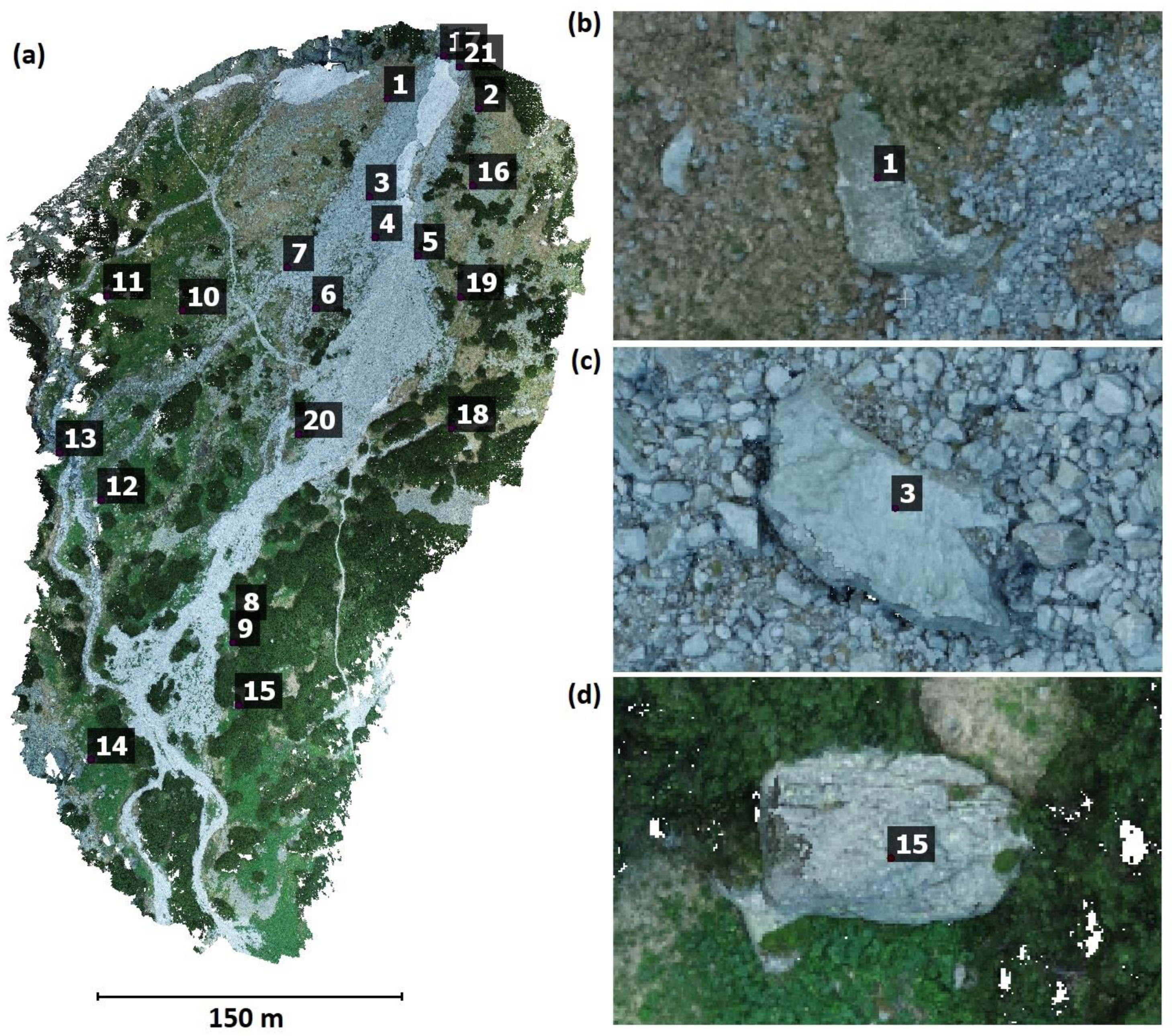A description of the TLS measurement and processing methodology is beyond this paper’s scope and can also be found in [49]. A second epoch (2022) check was then carried out by picking the coordinates of large boulders or rock outcrops in the plumes that were not displaced (see Figure 5). In most cases, these points lay outside the main flow of the landslide. A total of 21 suitable points were found in these areas. The height coordinates between the epochs were compared. The mean differences, standard deviations, and overall root mean square difference (RMSD) characteristics were determined.

2.8. Procedure Comparing Point Clouds from Epochs 2018 and 2022 with Determining Changes

The point clouds, as a result of processing, contained a high number of points. In addition to points that can be used for further processing (especially points on rocks or stones), some points cannot be used for further processing, especially those representing vegetation. Therefore, the processing was carried out as follows:

• The rasterization of point clouds, with a cell size of 0.05 m;
• The removal of green vegetation using the vegetation index ExG;
• Generating a mesh representation of the DTM from the 2018 data;
• Determining the elevation changes of the 2022 data compared to the 2018 DTM.

Rasterization was chosen as the initial manipulation because it reduces the number of points. Meanwhile, DTM singularities (points on top of each other or overhangs) were removed, thus greatly simplifying further processing (both the mesh area generation and the subsequent comparison). At the same time, it cannot be assumed that a change worthy of being recorded occurred in the natural environment in an area smaller than 0.05 m. Rasterization was performed in CloudCompare v 2.12.4. The starting point of the rasterization was manually set to be the same for both datasets.

Vegetation removal was necessary before data processing, as its presence biases the results. The changes could only be assessed in places where there was no vegetation at either stage. However, the vegetation, in this case, was dense and virtually impenetrable, and there were no points on the ground. Thus, it could not be identified by the geometric filters commonly used for this task, e.g., [50], nor by structural filters [38]. However, it could be distinguished based on color. A well-known description of greenness is the vegetation index, which can be used for this. The removal of green vegetation using the ExG (Excess Green, [51]) vegetation index was performed according to [40]. We chose ExG because e.g., in [52] (and also in other studies and our testing), it was performed the best of all tested methods. The ExG vegetation index shows the (simplified) amount of green color in a given color characterization of a point described by the visible color components R, G, B. The value of the ExG was determined for each point by the formula ExG = 3(2G-R-B)/(R+G+B). Generally, non-green has a lower index value, while green has a higher one. Once a threshold value was determined (dependent on the actual conditions, i.e., for each data point separately), points with a higher ExG value than the chosen threshold were removed. The calculation was performed in CloudCompare v 2.12.4 using the Arithmetic calculation function for working with scalar arrays. The procedure did not remove all unwanted points but significantly simplified the subsequent data filtering.

The following processing step was generating the mesh surface from the base epoch (2018 data). Given the performed rasterization, this process was carried out again using CloudCompare software.

The height changes could be determined by comparing the point cloud of the 2022 epoch with the mesh DTM representation of the 2018 data (CloudCompare, Compute cloud to mesh distance function). The advantage of this comparison is that the differences obtained were signed (unlike the cloud-to-cloud comparison). As a result, the obtained height differences could be suitably represented by colored hypsometry.

3. Results

The calculation results in two-point clouds from measurements in 2018 (2018 data) and 2022 (2022 data). The 2018 cloud has 216 million points, while the 2022 cloud has 168 million (see Figure 6).

The results of the internal consistency check of the photogrammetric models, i.e., the cumulative deviations of the GCPs after optimization, are shown in

Table 1. Residuals on GCP after SfM reconstruction.

Data	RMSE X (m)	RMSE Y (m)	RMSE Z (m)
2018	0.005	0.009	0.004
2022	0.013	0.015	0.009

.

After rasterization and the removal of the green vegetation points, point clouds were obtained for further processing, which had 26,833,928 points after rasterization and 11,285,776 points after green removal for the 2018 data, and similarly, 31,469,352 points and 15,460,209 points for the 2022 data (see Figure 7). It is clear here that there was a significant reduction by rasterizing and removing the green vegetation points.

3.1. Results of Verifying the Correct Georeferencing of Point Clouds from Both Stages

The primary validation of the deployment of the UAS SfM photogrammetry method in the alpine terrain is described in detail in [49]. The first epoch 2018 was compared here with the terrestrial laser scanning results. Based on this testing, the point cloud height accuracy of the 2018 stage can be described by an RMSE of 0.032 m (mean difference of 0.008 m, standard deviation of 0.032 m). A height comparison of the 2018 and 2022 epoch clouds at the 21 points selected at locations with unlikely displacement resulted in a mean difference of 0.016 m, with a standard deviation of 0.017 m. The overall RMSD value reached 0.024 m.

These results, at the stated level of accuracy, are undoubtedly sufficient to detect and describe in detail the changes that may occurred at landslide and rock field sites

3.2. Point Cloud Comparison Results from Stages 2018 and 2022

The result of comparing the 2022 and 2018 stages (2022 minus 2018, as 2018 was the base epoch) was a 2022 point cloud, with specified deviations in the form of a scalar field, which can be most easily expressed by a hypsometric scale (see Figure 8 and Figure 9). This form preserves the spatial distribution of the points. Beyond this, the variations can still be represented using a difference model, where each point’s position is kept, but its height is determined as the difference between the two models being compared.

Although these two expressions similarly describe the changes in color, in the differential model, the changes can be more easily expressed as isolines. Figure 10 shows the details of the three selected smaller areas. The color scale and isolines provide another expression of the morphological changes in the monitored area. Selected cross-sections supplemented with a graphic scale are also included.

Vertical cross-sections perpendicular to the general direction of the talus cone were extracted from the point clouds of both research epochs. The interval between the cross-sections was 10 m. They are shown in Figure 11a,b. The main tidal flow’s bed was derived based on these cross-sections. The lines in Figure 11a,b show the axis of the stream bed. Figure 11c shows a combined view of the main flow’s position change. Significant changes are visible in the cross-sections of the three selected details (Figure 11d–f).

4. Discussion

The research carried out in the locality of the Small Cold Valley confirms the results of the research by several authors, e.g., [53,54,55,56,57,58]. UAS-SfM photogrammetry was verified as a suitable and accurate method for monitoring geological processes and phenomena, such as morphological changes on debris cones, landslides, river erosion, rock falls, and other geohazards, even in highly complex high-mountain terrain. When following our described methodology, centimeter-level accuracy can be achieved. In the case of our measurements, an RMSD of 0.024 m between stages was obtained, a value that is better than expected. Furthermore, the comprehensive capture of the surface of the study area allowed for a very detailed evaluation of the changes between two or more of the observed epochs.

In our case, the objective was to monitor changes in the debris cone caused by water erosion during significant tidal rainfall events. The first measurement, carried out in 2018, captured the debris cone in detail, and thus, provided us with a basis for regular monitoring. In the period of 2018–2022, several significant rainfall events occurred in the area of interest, characterized as torrential rain with a total rainfall of more than 50 mm in 24 h. Before the realization of epoch 2022, we anticipated that these significant rainfall events would likely have caused a change in the morphology of the debris cone. 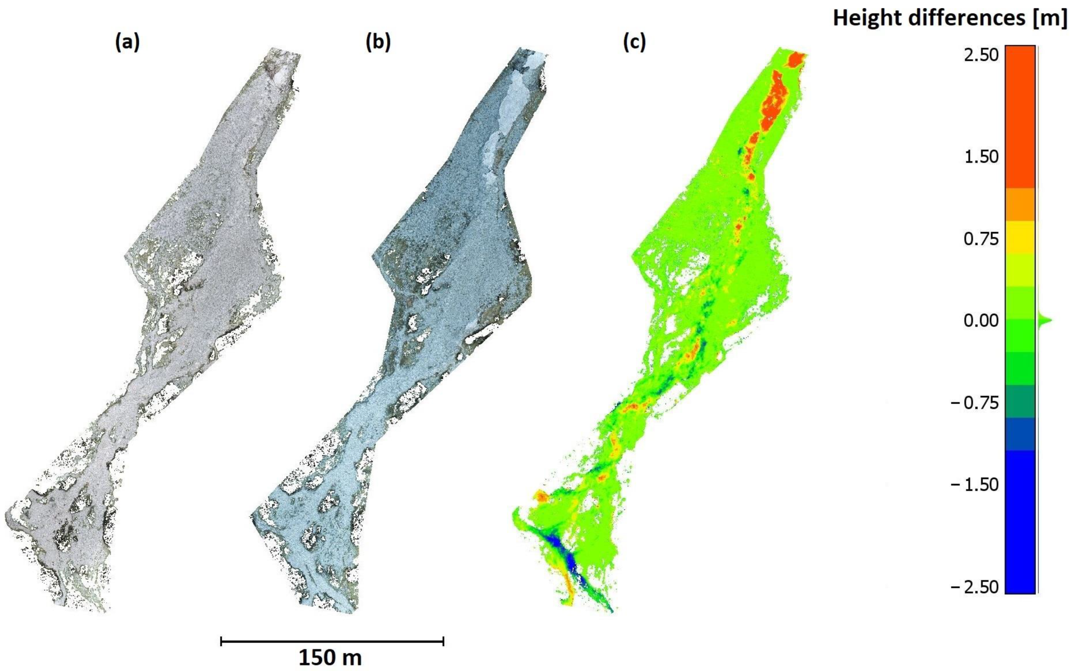We also expected a change in the mountain stream bed that flows in the lower part of the debris cone (see Figure 12). These changes in the field were visually identified based on the 2018 photographs and the 2022 ground conditions but were not accurately confirmed by the measurements. From the geology, hydrology, and sedimentology perspectives, we hypothesized that sediment was transported from the upper parts of the debris cone downslope that occurred during 2018–2022, in addition to altering the actual shape of the stream channel in some areas. In particular, the width and depth of the channel bed changed, replacing the riparian banks with alluvial banks and vice versa. These processes are typical of headwater streams, especially in high mountain environments, where the stream ‘seeks the path of less resistance’, and thus, often changes its channel. All of these assumptions have been demonstrated in our research. The processes have been identified in the models created by merging or differencing the 2018 and 2022 models. Stream meandering, the formation of alluvial deposits, and significant lateral erosion are clearly visible in the difference models in Figure 8c and Figure 9c. The red areas represent the alluvial banks, and the blue areas the eroded parts.

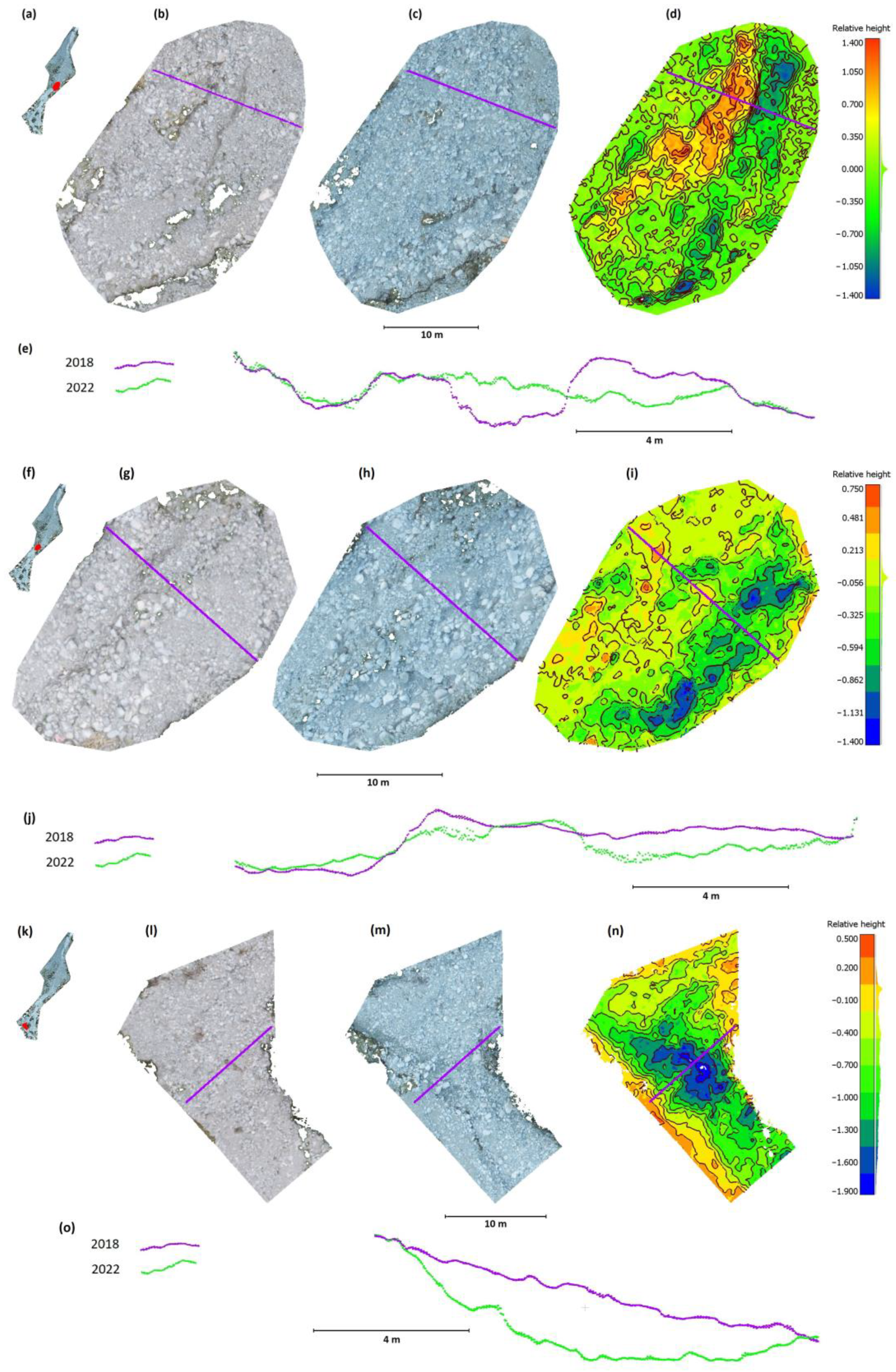
Figure 11 shows the morphological changes on the talus cone in detail. In some parts of the debris cone, significant changes to the cone relief can be seen in the cross-sections.

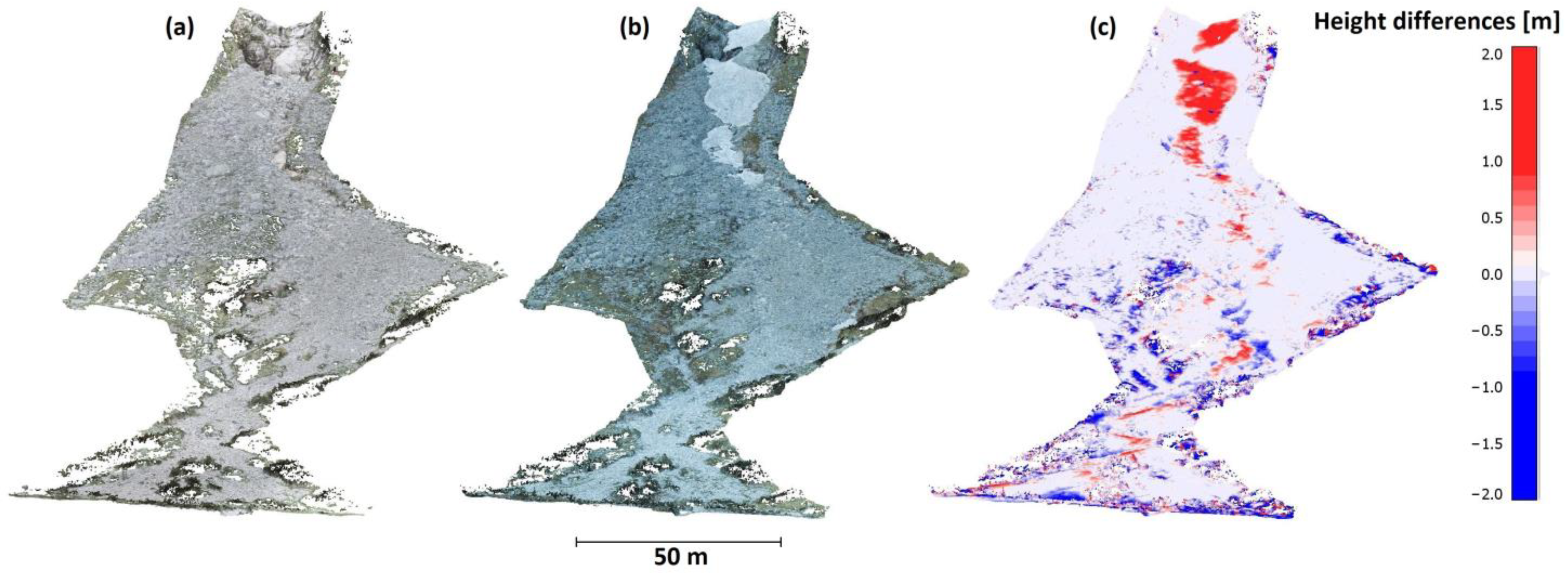
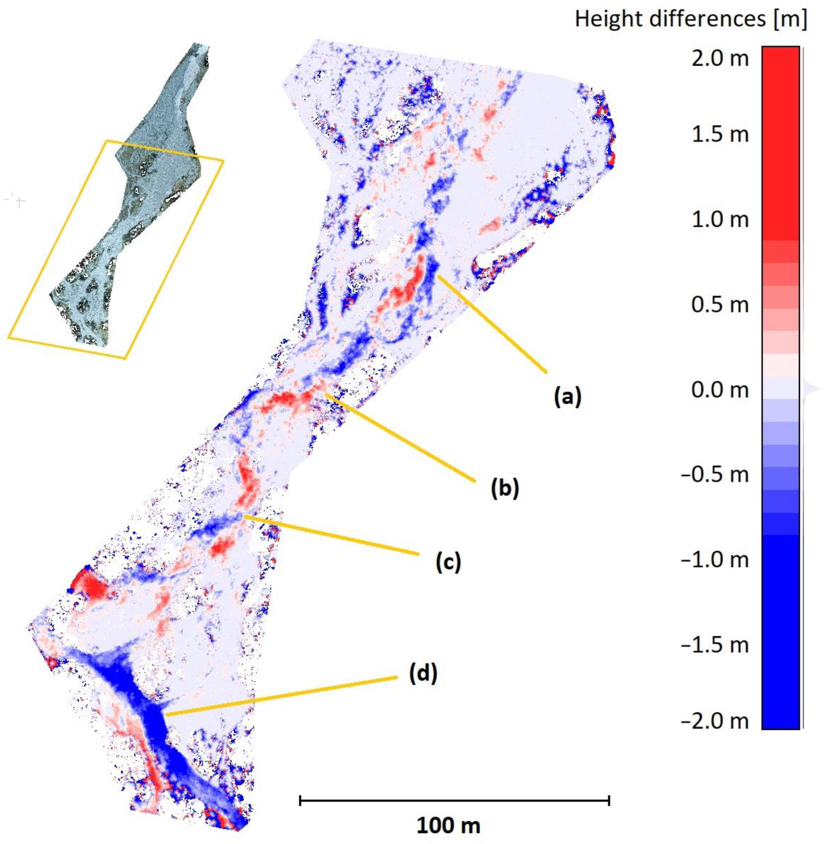
The changes were the most significant in the lower part of the debris cone, shown in detail in Figure 12. Blue areas indicate the places with significant erosion, and the red areas are where sediments of the cone were deposited. Figure 12a–c shows substantial changes due to material transport from the top of the debris cone. Increments in the upper part of the debris cone are also visible, but these were distorted by snow and ice remnants in 2022.

Figure 12d indicates an area where significant changes occurred. However, their origin was not due to the processes of the observed debris cone. They arose as the result of the action of the water of the main stream flowing through the floor of the valley.

This paper presents a comprehensive geodetic monitoring methodology and its practical application to a landslide zone formed by a rock field. The monitored area is located in the area of the national park with the highest protection, where practically any permanent installation of measuring equipment is prohibited, and therefore, it is not possible to place, e.g., geotechnical boreholes, inclinometers, etc. In this type of terrain, it is impossible to build a base for ground-based InSAR (according to [9,10]); the opposite slope from which monitoring could be carried out is also in the area of another debris cone. Due to the large movement of rocks, the deployment of relative geotechnical measuring instruments [3] is also unreliable as there is a high probability of destruction—as is evident from the documented changes in the Results section.

The UAV photogrammetry method was chosen for the staged measurements because of its high efficiency and cost and the character of the resulting data, as evidenced by a study [59] where several staged raids were carried out in the Italian Alps. The authors reported a relatively high accuracy in centimeters (0.02 m in position, 0.05 m in height), but they derived this only from the results of the SfM calculation, without an independent check and without knowing what errors occurred in the spaces between the GCPs. It can also be assumed that these were predominantly errors due to the measurement of the GCP coordinates by the GNSS-RTK receiver, which has roughly corresponding standard deviations. In our case, these values were halved for the position and quartered for the height, but the observed DMT standard deviation was worse (0.024 m between stages). The authors also did not report the precision setting for the SfM calculation, which significantly affected the resulting deviations on the GCP after the model’s calculation (which only characterized the model’s internal consistency with the GCP).

In [43], two different UAVs with cameras of different quality (DJI Matrice 600 with X5 camera (16 Mpix), and DJI Phantom 4 with a built-in camera (12 MPix)) were used for the stage monitoring of a landslide in the Western River. The flight height was 110 m above ground level. As a result, the DSM with a 0.04 m resolution was created. The authors used GNSS receiver measurements among other methods. In this paper, no comparison of the results was made to determine the spatial quality, and only the evaluation of changes (i.e., with unknown predictive power) was always performed. For example, the determination of changes through the DSM was carried by post-positioning the models on top of each other using the ICP algorithm, without considering that the areas affected by the changes necessarily affected the overall relative position of the clouds after transformation. This can only be avoided by a good-quality georeferencing of the clouds based on a network of stationary points (optimally determined by geodetic methods).

In [44], the monitoring of a small landslide (about 50 m × 50 m) in three stages by a multicopter UAS from a height of 70 m with GSD 0.02 m was presented. However, after calculating the SfM-MVS method, deviations of the GCP of 0.06 m–0.11 m were presented, which significantly exceeded the expected accuracy (in contrast to the GSD). No control methods were used to verify the accuracy of the results independently. A geometric filter (built-in Agisoft software) was used for vegetation filtering. Since the scene was mainly characterized by low vegetation and grass, it could not remove grass of different heights and only removed taller vegetation, thus biasing the comparison results.

In [45], extensive research on landslide monitoring along the Vallone dell’Elva Road (Italy) is presented. The monitored area is large (measuring about 5 km in length), and various instruments and techniques were combined, including UAS SfM-MVS and ground-based photogrammetry. The measurements were very detailed, and a DJI Phantom 4 was used for the UAS SfM imaging. The presented density of the point cloud was presented as an average GSD value of 0.04 m. A total of 39 GCPs were used for the calculation, and only 16 control points were used for the control. The control results are not shown, although the high accuracy of their determination (0.003 m) is declared.

In our opinion, given these studies, the correct methodology is crucial for determining appropriate conclusions and subsequent measures for slope remediation or predicting emergency conditions. Our study’s value goes beyond identifying GCPs precisely enough for stage comparisons. The control and oversight of the computing process, as well as the handling of point clouds, are equally crucial. Few studies have discussed, for instance, how to remove obstructing vegetative cover, which is essential for material transfer investigation.

We consider the methodology satisfactory regarding the achieved accuracy and detail of the researched area. To improve the methodology, maintaining a constant AGL flight definition, preferably using automatic mission, can be recommended. To improve the photogrammetric results, we recommend a higher camera quality. To reduce the amount of unmeasured places, there can be a recommended flight scheme with different orientations of the shot axes, e.g., as implemented by DJI for higher-class UASs (consecutive images are oriented vertically down, left, right, forward, backward, down, etc., e.g., the slope is always 30°).

5. Conclusions

Monitoring and evaluating landslide events is a team effort that must involve various engineering professions to ensure success. In particular, engineering geology, geotechnics, and geodesy can be mentioned. It is the geodetic part of the monitoring that we have dealt with in our article, and we have tried to describe the most important elements of its proper implementation.

Regardless of subsequent measurement technologies (such as lidar, 3D scanning, UAV photogrammetry, etc.), it is always necessary to ensure unambiguous inter-stage continuity, which, in principle, cannot be performed other than by classical geodetic measurement from a geodetic reference network that is reliably stabilized outside the area of changes.

Furthermore, it is necessary to carry out quality checks on the results in each measurement and processing step, otherwise, the quality of the deformation determination cannot be guaranteed when comparing the results of the stage measurements.

Last but not least, it is always necessary to carefully remove data from the measurements of individual stages that represent areas subject to non-landslide deformation effects, in particular the presence of vegetation that limits or prevents ground surface acquisition.

Based on the obtained results, we can state that the proposed UAS-SfM photogrammetry methodology is suitable for monitoring geological phenomena. It is also suitable for monitoring surface morphometric changes even in complex conditions in a high-mountain alpine environment [60,61]. Using the UAS photogrammetry method, we could detect changes at a range of centimeters. We could evaluate spatiotemporal changes in the terrain even in relatively inaccessible environments where other technologies, such as terrestrial laser scanning, cannot be effectively applied over a larger area. The above-described methodology’s implementation of the highest-quality geodetic network is essential because it serves as the basis for the individual epochs of measurement and subsequent evaluation. The points of the reference geodetic network should be located in areas where their stability is expected. Points creating a geodetic network would be more accurately determined than the data collection method itself. Using a total station to determine the reference points is very suitable, as it eliminates systematic errors between stages down to millimeters. The epoch measurements can then be used to obtain digital terrain models, for which it is necessary to remove the vegetation for further analysis. Vegetation filtering can be very problematic in landslide areas for many geometric filters due to the extreme ruggedness of the terrain. However, filters that work with the vegetation index based on the color information of individual points can preferably be applied. Applying the correct methodology then allows for an epoch-by-epoch comparison. Subsequently, an analysis of material loss and gain can be obtained with precise localization, which aids in understanding the erosive processes of rainfall events in landslides and rockfalls.

In our current and previous research, we investigated the limits of the methods and the quality of the results of the spatial data obtained by several measurement methods, including TS, GNSS, TLS, ALS, and photogrammetry. In future work, as a terrestrial approach, we plan to deploy mobile mapping based on lidar with georeferencing using RTK GNSS (e.g., the Leica Pegasus backpack) [62] and technology based on SLAM, e.g., Leica BLK “to go” [63]. Among the remote sensing methods, we are considering monitoring using INSAR.