Comparing the Trajectory of Urban Impervious Surface in Two Cities: The Case of Accra and Kumasi, Ghana

Abstract

In this study, we present methods to assess newly developed urban impervious surface (UIS) datasets derived from satellite imagery of the cities of Kumasi and Accra, Ghana, at three different time points. Each city has three binary maps from 2000, 2011, and 2021, in which one shows the presence of UIS and zero shows its absence. We employed the binaryTimeSeries method to compare the gross gains and losses in the two cities. In addition, we show how three components of change—quantity, allocation, and alternation—compare across the two sites. The results show that both cities experienced a large proportion of gains during the change in impervious surfaces between 2000 and 2011, and 2011 and 2021, with relatively smaller loss proportions and alternations. Comparatively, the results from the components of change show that change is fastest in Kumasi, which had a larger proportion of quantity gain. Our methods show an acceleration in UIS in the two cities during the temporal extent, and this trend is likely to continue with increasing urban populations. As a result, we recommend that the Land Use and Spatial Planning Authority, Town and Country Planning and other stakeholders make contingency plans to regulate the unplanned increase in UIS, since other studies have shown their negative effects on people and the environment.

1. Introduction

Globally, the increasing number of people living in urban areas has grown rapidly over the past two decades. In 2000, 3.5 billion people, comprising 46% of the global population, settled in urban areas, and this number increased to 54% (4 billion) in 2015. Projections are that 6 billion people (~60% of the world’s population) will reside in urban areas by 2050, and more than 90% of this growth will occur in Asia and Africa [1]. Scientists and stakeholders have employed urbanization levels as proxies for economic development, modernization, and the capacity of people to transform natural environments into built environments. However, the increasing urbanization levels result in urban impervious surface expansion (UISE). The UISE significantly contributes to cropland reduction [2,3], air pollution [4,5,6], greenhouse gas emissions [7,8] and increasing land surface temperature [9,10,11]. Thus, there is an increasing need to generate reliable data and metrics to study the changes associated with impervious surface expansion.

Admittedly, remote sensing has provided data for developing global-, regional-, national-, and local-level products to monitor and detect urban impervious surface area expansion. However, the global products underestimate the urban extents in Africa, and the existing regional-level data in Africa are only available at 2 km resolution, meaning we could not detect subtle changes in urban areas. Moreover, the national-level and local-level products use different image classification methods, including maximum likelihood, a support vector machine, and random forest, to create urban change maps, making it difficult to make comparative change analyses [12]. Regardless, remote sensing has provided Earth observation data that facilitates the quantification and analysis of urban impervious surface change over time.

Methods to measure the change in urban impervious surfaces abound. However, these methods have two main drawbacks. First, the methods only measure the net change and, as a result, fail to show the gross gains and losses that contribute to the net change. For instance, Ref. [13] used annual time series Landsat data to measure the spatiotemporal dynamics of impervious surfaces in Guangzhou, China. Their study used a time series graph to show the sizes of impervious surfaces at each time point, which facilitates the measurement of the net annual change but not of gross losses and gains. Second, existing methods compare change during a single time interval, even when data are available for more than two time points. Mugiraneza et al. [14] suffered the same drawback when they used a time series graph to measure the change in urban land cover in Kigali, Rwanda.

Other studies have employed the transition matrix to circumvent the time series graphs’ drawbacks. The transition matrix allows scientists to compare change during a time interval. A time interval is the duration between two time points; thus, the transition matrix compares the change between an initial and a subsequent time point. For example, Ref. [15] used the transition matrix to develop a metric to measure quantity and allocation disagreements among land cover categories. Similarly, Ref. [16] extended the transition matrix to create intensity analysis—a framework that measures the intensities of change in categorical variables at the interval, categorical and transitional levels. The original framework of intensity analysis inspired the authors of [17] to develop component intensities that facilitate the comparison of each category with other categories and their overall differences.

Intensity analysis and its cohort of derived metrics have gained currency in studies concerning urban change and, by extension, urban impervious surfaces. For instance, Ref. [18] used intensity analysis to study the patterns and process of slum growth in Lagos, Nigeria, between 2009 and 2015. Feng et al., Manzoor et al., Abass et al., and Gandharum et al. [19,20,21,22] echo the popularity of intensity analysis in their studies concerning land change. Despite its popularity, intensity analysis has one major shortcoming—it is limited to studies considering change between two time points. On the other hand, examining change beyond two time points provides tremendous opportunities for unearthing critical information such as alternation, which can indicate data errors or the oscillation of the change [23].

Therefore, we propose a new metric to help city governments, planning institutions, and stakeholders interested in UISE dynamics make informed urban land use decisions. Bilintoh and Pontius, Jr. [23] developed a metric and the binaryTimeSeries R package to measure the change in the trajectories of a binary variable during a time series. The metric allows scientists to measure gross losses and gains during a time series and facilitates cross-site comparison.

2. Materials and Methods

2.1. Study Sites

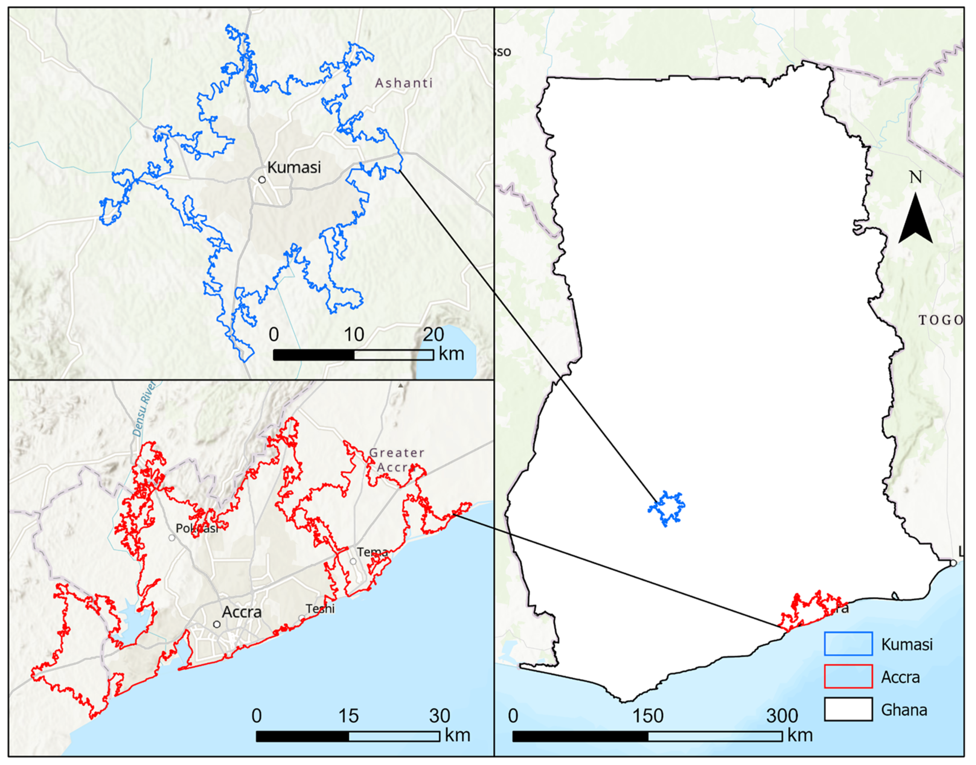
Accra, the capital of Ghana and the Greater Accra Region, occupies an area of 225 square km with a population density of 129 people per square km. Kumasi, the capital of the Ashanti Region, covers an area of 230 square km with a population density of 223 people per square km (see Figure 1). Between 2010 and 2021, Accra’s population increased by 2.1% annually, while Kumasi’s grew by 1.2%. These two cities, which are about 270 km apart, are the two largest cities in Ghana and have been the focus of infrastructure investments from governments and investors, both local and foreign.

The concentration of economic, educational, and health facilities attracts people to these cities, resulting in growing urban populations and a demand for housing. The demand for housing has resulted in speculative developments, where people are developing in anticipation of profits. Additionally, many new developments are emerging in these cities in response to globalization and the real estate turn in major African cities [24,25,26]. Consequently, the majority of foreign (in)direct investments flow into Accra and Kumasi, and this is made possible through the privatization of communal lands [27]. Although the two cities have substantially increased their areas over the past 20 years, comparative studies are lacking, partly due to the inconsistent and city-level characterization of UIS. Therefore, knowledge of UIS trajectories between the two largest cities in Ghana can potentially inform sustainable city-level urban planning and management.

2.2. Data Source and Preparation

In this study, we used the United States Geological Survey (USGS) Landsat 7 Enhanced Thematic Mapper Plus (ETM+) and the Landsat 8 Operational Land Imager and Thermal Infrared Sensors collection 2, tier 1, level 2 science products. First, we used a date filter to retrieve all Landsat images acquired for 2000 (24 images), 2011 (25 images), and 2021 (94 images), and applied a median reducer to generate a single image for each year. Due to the different bandwidths between Landsat 7 and 8 sensors, we harmonized the two using coefficients in [28]. We then used the CFMASK algorithm to mask clouds and cloud shadows. We generated an annual collection of four indices, including the normalized difference built-up index [29], normalized built-up index [30], normalized built-up area index [31], and built-up [32] for each of the three years.

We generated random points within the city boundaries of Accra and Kumasi and created a gridded 30 × 30 m pixel around each point. Using Google Earth Pro 7.3, we estimated the urban impervious area percentages of 435 points, resulting in 52 points in 2000, 158 points in 2011, and 225 points in 2021. We partitioned the samples into 70% for training (305 points) and 30% (130 points) for validation.

Next, we used Google Earth Engine to generate a continuous urban impervious cover using a random forest regression model, which estimates the relationships between the urban spectral indices and the interpreted points from Google Earth.

2.3. Methodology

Bilintoh and Pontius, Jr. [23] developed methods and the binaryTimeSeries R package to analyze the trajectories of a binary variable during a time series. We employed their methods and the R package to analyze the trajectories of UIS in the two cities. Equations (2) and (3) show how to compute the gains and losses of the variable, considering its trajectories as a proportion of the product of the duration of time interval t, and the number of locations for the trajectory j. The size of the unified region ($U$), which facilitates site comparison, is the union of all pixels that show the presence of the variable during temporal extent. $d_t$ annualizes the results. Equations (4) and (5) show how to compute the average loss and gain during the temporal extent. Then, Equations (6)–(9) compute the three components of change: quantity, allocation, and alternation. The quantity component measures the net change from the initial time point to the final time point of the time series. The allocation measures the simultaneous gain in some locations and the loss in other locations from the initial time point to the final time point of the series, which the net change does not reveal. Alternation occurs when a pixel experiences one or more pairs of loss and gain during the time series.

Table 1. Description of the six types of trajectories.

Code	Change Trajectory	Color	Definition
0	Mask	White	Eliminated from computation
1	Loss without Alternation	Dark Red	Y1m0 > Y1mT and Y1mt−1 ≥ Y1mt for all t
2	Gain without Alternation	Dark Blue	Y2m0 < Y2mT and Y2mt−1 ≤ Y2mt for all t
3	Loss with Alternation	Light Red	Y3m0 > Y3mT and Y1mt−1 < Y1mt for at least one t
4	Gain with Alternation	Light Blue	Y4m0 < Y4mT and Y1mt−1 > Y1mt for at least one t
5	All Alternation Loss First	Dark Yellow	Y5m0 = Y5mT and loss is first change
6	All Alternation Gain First	Light Yellow	Y6m0 = Y6mT and gain is first change
7	Stable Presence	Dark Gray	Y7mt−1 = Y7mt ≠ 0 for t = 1, 2, …, T
8	Stable Absence	Light Gray	Y8mt−1 = Y8mt = 0 for t = 1, 2, …, T

and

Table 2. Mathematical notations for equations.

Symbol	Meaning
dt	Duration of time interval from time t − 1 to t where dt > 0
Gjt	Annual gross gain as a proportion of the unified region in trajectory j from time t − 1 to t where Gjt ≥ 0
J	Index for trajectory where j = 1, 2, 3, 4, 5, 6, 7, 8
Ljt	Annual gross gain as a proportion of the unified region in trajectory j from time t − 1 to t where Ljt ≤ 0
M	Index for an observation in trajectory j where m = 1, 2, …, Mj
Mj	Number of observations in trajectory j
St	Size of presence in the binary category at time t
t	Index for a time point where t = 0, 1, 2, …, T
T	Number of time intervals where T ≥ 1
U	Size of the unified region
vt	Annual net change proportion from time t − 1 to t in Equation (3)
Yjmt	Value of binary variable in trajectory j at location m at time t

describe the trajectories and provide notations concerning Equations (1)–(11). Finally, Equation (10) shows how to compute the size of presence in the binary category at time t, while Equation (11) shows how to compute the annual net change proportion from time t − 1 to t in Equation (3). As [23] intimated, it is impossible to see trajectory types 3 and 4 for datasets with time points less than 4. Thus, our results reflect only six trajectories. The six trajectories are as follows: (1) loss without alternation, (2) gain without alternation, (3) all alternation loss first, (4) all alternation gain first, (5) stable presence, and (6) stable absence.

$$U={{\displaystyle \sum }}_{j=1}^7{M}_j$$

(1)

$$L_{jt}=\left[{{\displaystyle \sum }}_{m=1}^{M_j}\mathrm{MINIMUM}\left(0,Y_{jmt}-Y_{jmt-1}\right)\right]/\left(U{d}_t\right)$$

(2)

$$G_{jt}=\left[{{\displaystyle \sum }}_{m=1}^{M_j}\mathrm{MAXIMUM}\left(0,Y_{jmt}-Y_{jmt-1}\right)\right]/\left(U{d}_t\right)$$

(3)

$$\mathrm{Loss} =\left[{{\displaystyle \sum }}_{j=1}^6{{\displaystyle \sum }}_{t=1}^T\left(L_{jt}{d}_t\right)\right]/\left({{\displaystyle \sum }}_{t=1}^T{d}_t\right)$$

(4)

$$\mathrm{Gain} =\left[{{\displaystyle \sum }}_{j=1}^6{{\displaystyle \sum }}_{t=1}^T\left(G_{jt}{d}_t\right)\right]/\left({{\displaystyle \sum }}_{t=1}^T{d}_t\right)$$

(5)

$$\mathrm{Net} = \mathrm{Loss} + \mathrm{Gain}$$

(6)

$$\mathrm{Quantity} =\left|\mathrm{Net}\right|=\left|{{\displaystyle \sum }}_{j=1}^4{{\displaystyle \sum }}_{m=1}^{M_j}\left(Y_{jmT}-Y_{jm0}\right)\right|/\left(U{{\displaystyle \sum }}_{t=1}^T{d}_t\right)$$

(7)

$$\mathrm{Allocation} =\left[\left({{\displaystyle \sum }}_{j=1}^4{{\displaystyle \sum }}_{m=1}^{M_j}\left|Y_{jmT}-Y_{jm0}\right|\right)/\left(U{{\displaystyle \sum }}_{t=1}^T{d}_t\right)\right]- \mathrm{Quantity}$$

(8)

$$\mathrm{Alternation} = \mathrm{Gain} - \mathrm{Loss} - \mathrm{Allocation} - \mathrm{Quantity}$$

(9)

$$v_t=\frac{S_t-S_{t-1}}{U{d}_t}$$

(10)

$$S_t={{\displaystyle \sum }}_{j=1}^7{{\displaystyle \sum }}_{m=1}^{M_j}{Y}_{jmt}$$

(11)

3. Results

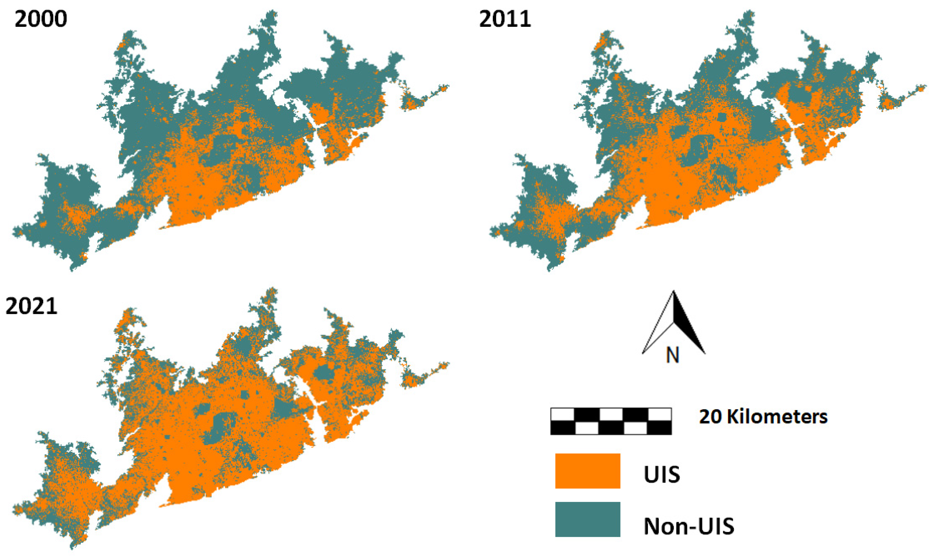
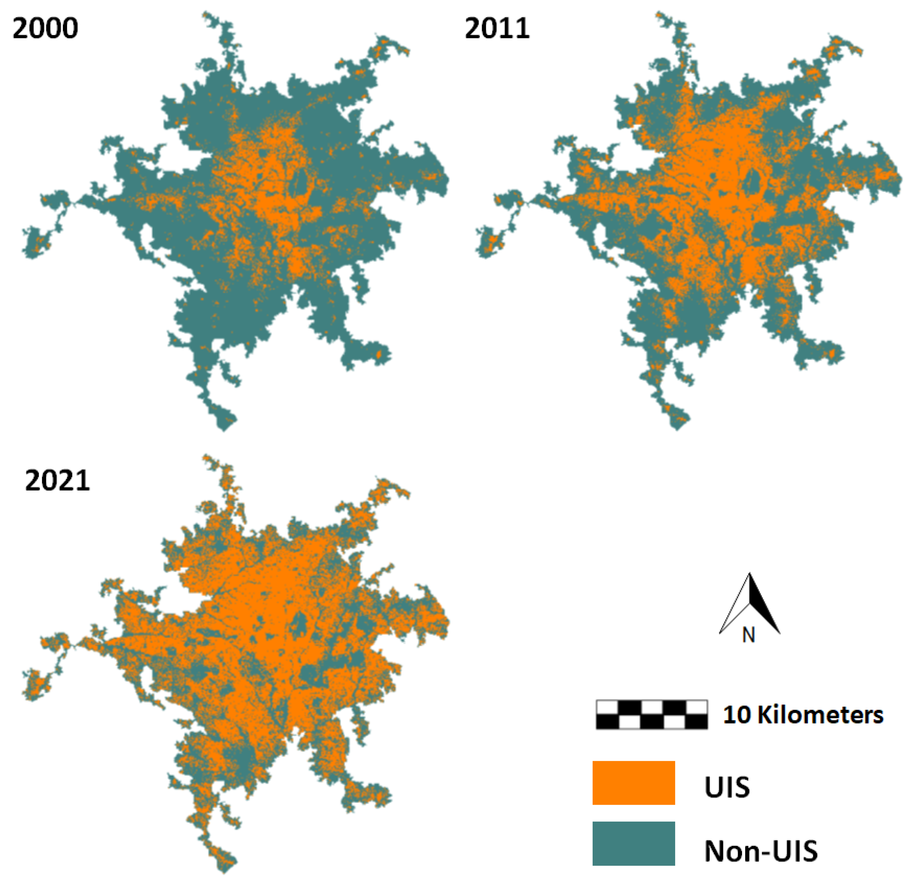
For our binary analysis, we classified the continuous urban impervious cover into two binary classes: urban impervious surfaces with pixel values greater than 20 percent, and non-urban impervious surfaces with pixel values less than or equal to 20 percent (Figure 2 and Figure 3). UIS have a 0.1739 commission and a 0.0952 omission error, while non-UIS have a 0.0984 commission and a 0.1791 omission error. The errors for UIS and non-UIS are balanced, meaning we neither overclassified nor underclassified each class.

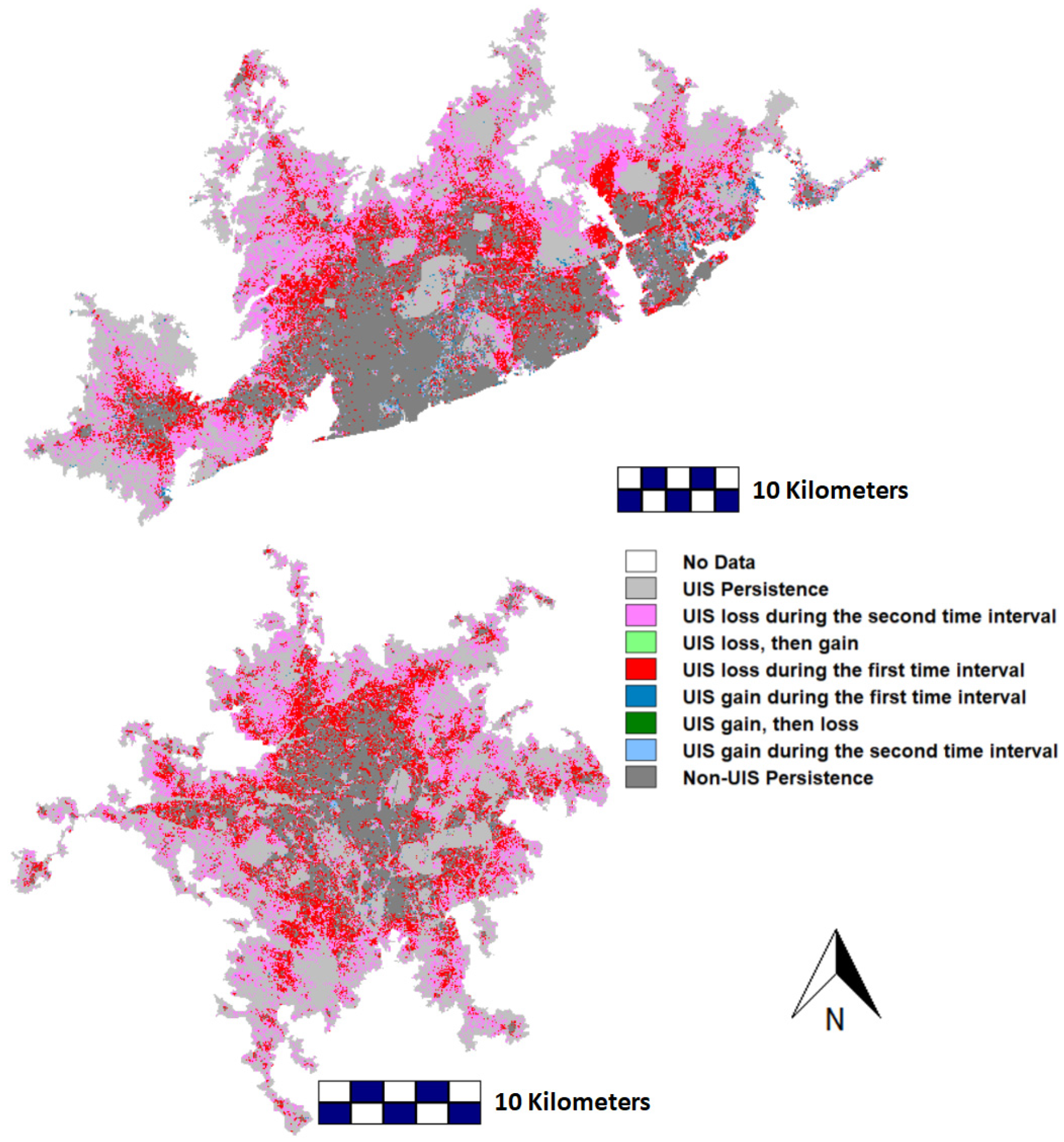
Figure 4 shows a three-way map overlay for each study site. For each region, we analyzed maps at three time points. Therefore, the maximum number of times UIS can exist is three, which reflects UIS persistence. The map in Figure 4 shows a concentration of UIS persistence in the southern parts of Accra. These areas are along the coastal areas. Conversely, most of the change in UIS (all other colors except white and the two shades of gray) occurs in the northern parts of the map. The persistence of UIS in Kumasi turns into a cluster in the central part of the region and is flanked by other changes in a random pattern. UIS loss during the first time interval and UIS loss during the second time interval dominate the changes in both regions, with the latter occurring closer to UIS.

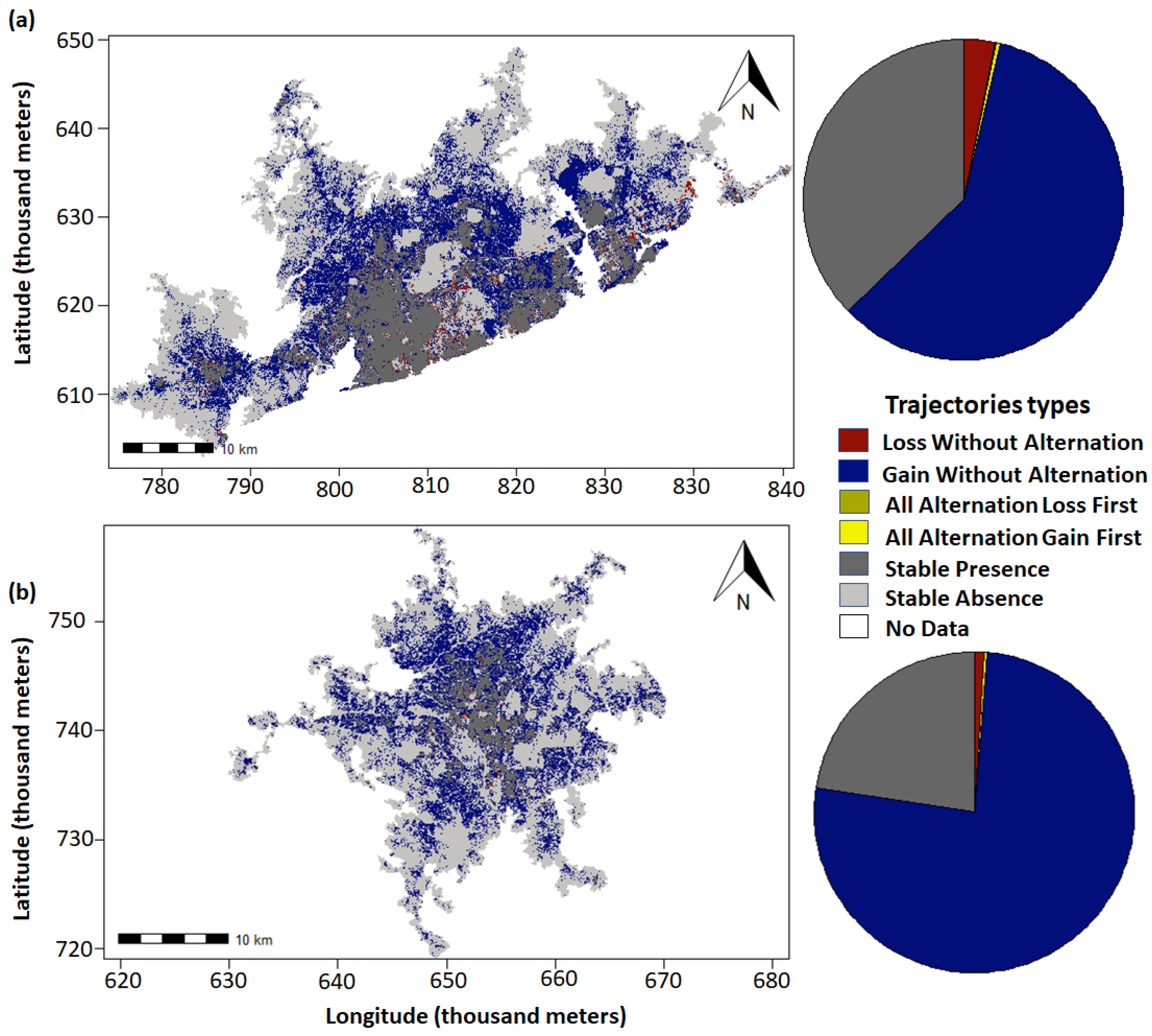
Figure 5a,b show the spatial distributions of the trajectories of change. Although the legend shows six trajectories, only four are visible on the map because of the relatively small number of pixels representing the two shades of yellow. Indeed, the pie charts show a slider in yellow, which is difficult to see.

Table 3. Sizes of trajectories that constitute the unified region in Accra.

Trajectory	Number of Pixels
Loss Without Alternation	21,634
All Alternation Loss First	253
All Alternation Gain First	3021
Gain Without Alternation	401,352
Stable Presence	252,695

and

Table 4. Sizes of trajectories that constitute the unified region in Kumasi.

Trajectory	Number of Pixels
Loss Without Alternation	2280
All Alternation Loss First	46
All Alternation Gain First	808
Gain Without Alternation	188,367
Stable Presence	55,796

show the number of pixels for each trajectory. Overall, the maps show that absence–gain–absence accounts for most of the change in both regions.

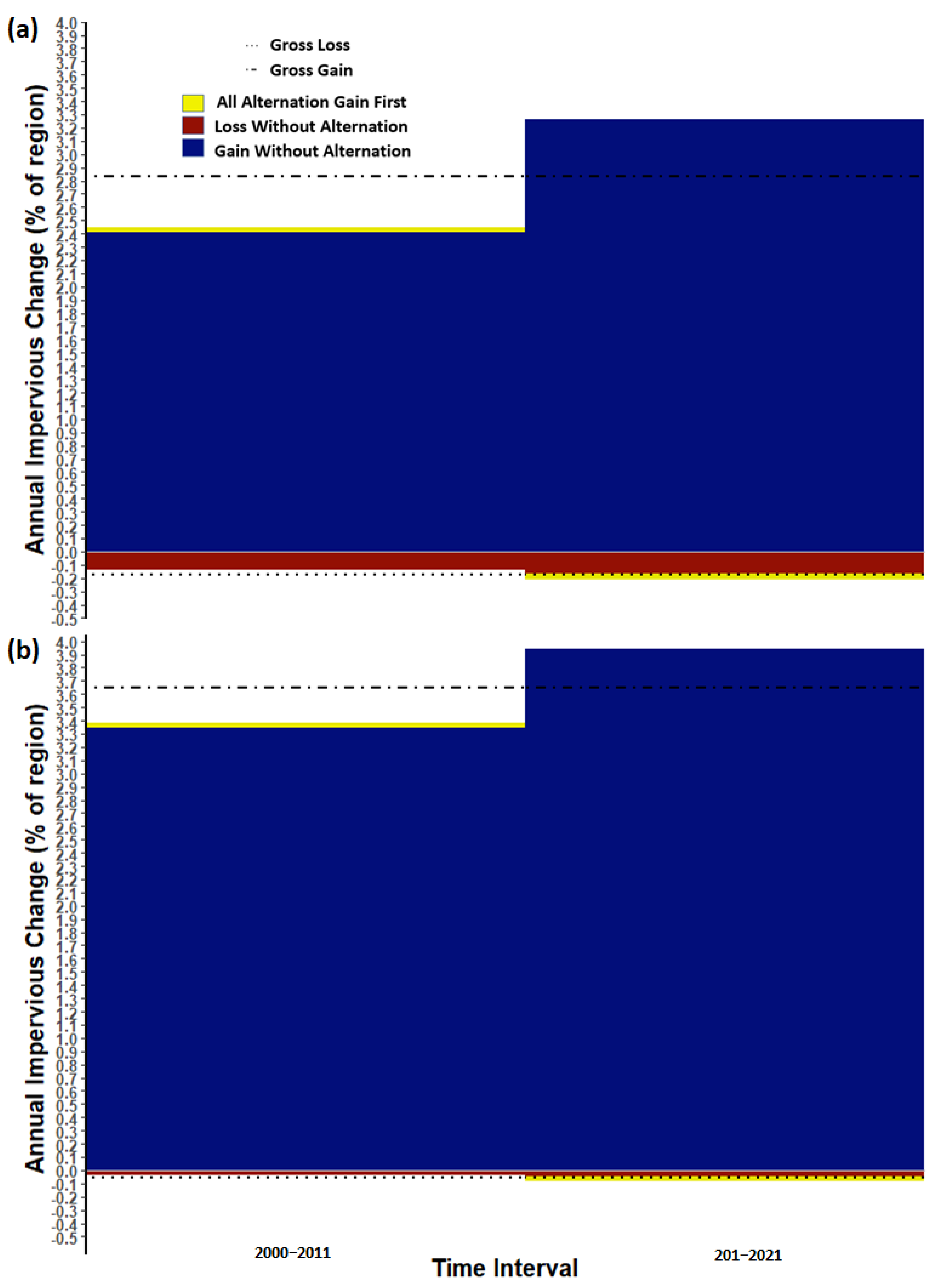
The stacked bars in Figure 6a,b show the impervious surfaces’ gross gains and losses in Accra and Kumasi during the temporal extent. The gross gains are above the time axis, which is at the 0-mark line, while the gross losses are below. In addition, the stacked bars partition the temporal change into time intervals, where 2000–2011 constitute the first time interval and 2011–2021 constitute the second time interval. Thus, the trajectories appearing during a time interval denote their contribution to the size of the trajectory. For instance, absence-alternation-absence appears as a gain during the first time interval and as a loss during the second time interval. We interpreted the yellow in the first time interval as how much the first time interval contributes to the size of absence-alternation-absence during the temporal extent. Intuitively, we interpreted the yellow segment in the second time interval as to how much the second time interval contributes to the size of absence-alternation-absence during the temporal extent. The proportion of the darker shade of yellow is approximately 0; thus, it does not appear on the stacked bar. Figure 6a,b show that gains account for most of the change in Accra and Kumasi. Furthermore, the stacked bars reveal that the range of the segments is greater during the second time interval, indicating that change accelerated in both sites. The gross loss and the gain line show the annual average loss and gain, which we interpreted as the change we may observe if the losses and gains occur uniformly. Therefore, the difference between the gross loss and gain lines communicates the net change.

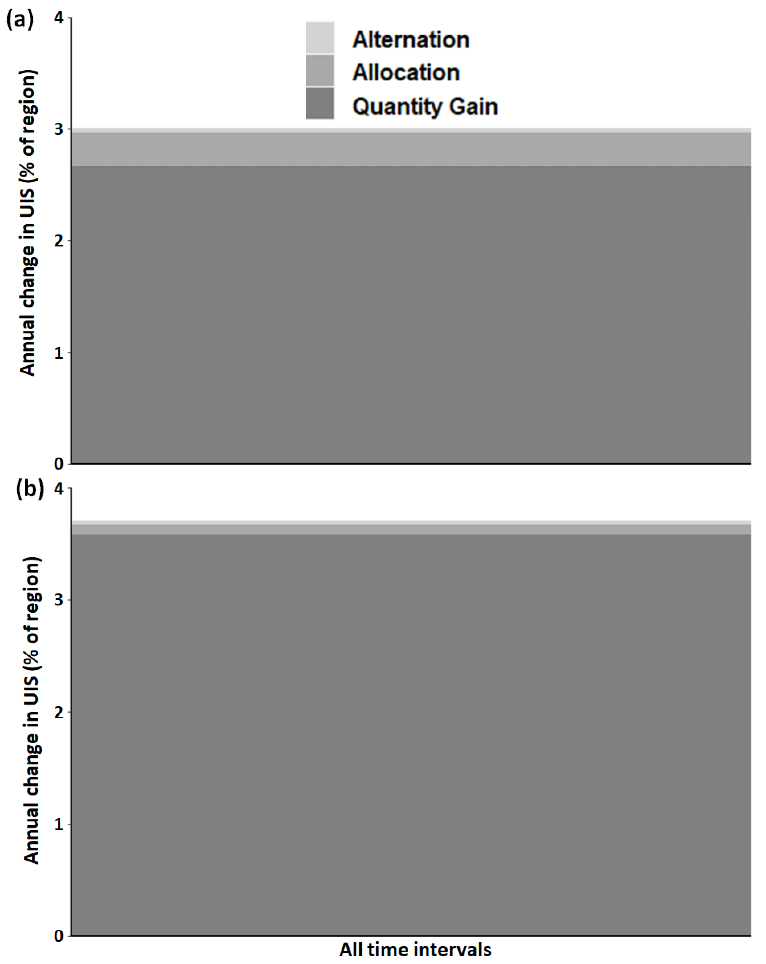
Figure 7a,b show the sizes of quantity, allocation, and alternation during the temporal extent. Quantity gain occurs when gross losses < gross gains. Quantity loss occurs when the reverse is true. Figure 7 shows that quantity gain accounts for most of the change in both sites, with Kumasi having a greater size of quantity gain. Despite having about an equal amount of alternation, allocation is greater in Accra. Overall, the range of the stacked bar in Figure 7b is greater than that in Figure 7a. As a result, change is faster in Kumasi.

4. Discussion

4.1. Unified Region Facilitates Site Comparison

Scientists have developed and applied several equations to studies concerning urban change. FAO and Puyravaud [33,34] are popular among these equations. Both are exponential equations; thus, we can assume that the patterns in the data are exponential. However, [23] described the limitations of these equations. We will reiterate the pitfalls of the changing denominators for emphasis. FAO and Puyravaud [33,34] proposed exponential equations with the initial variable size in the denominator. This creates two sets of complications: (1) the equations assume growth from zero is impossible, and (2) the initial size can vary for multiple time intervals. The former is a fallacy because some land cover classes can exhibit growth from zero. For example, a landscape might have an absence of urban areas during the initial time point and a presence of urban areas during the subsequent time point, which will result in a positive change in the urban area. The latter makes it difficult to compare change across time intervals and sites because of a changing base, as [23] intimated. $U$ in Equations (2) and (3) rectifies the problems associated with a varying denominator. Specifically, $U$ is constant during all time intervals and can only be unique for multiple sites.

4.2. Trajectories of Gross Loss and Gains

Urban impervious surfaces stem from several factors and may either provide solutions to a country’s development or be its Achilles’ heel. For instance, a country might intensify its infrastructure development through the construction of roads, hospitals, housing units, electricity power stations, and airports, in response to the demand for economic development. These infrastructures stimulate urbanization and require impervious surfaces [35,36]. Accra, the capital region of Ghana, has witnessed an influx of people seeking greener pastures, leading to an increase in the demand and supply effects of infrastructure during the 20th century [37,38]. This is evident in Figure 7, which shows UIS accelerated during the temporal extent. Ref. [39] reports similar trends in their study about the causes of flooding in Accra, Ghana. Their study identified an increase in impervious surfaces as one of the contributing factors to flooding in Accra. Amoako and Boamah [39] quantified the urban sprawl in Accra from 1985–2014 and reported an annual increase of about 7.8% in urban development. Similar studies show that the narrative in Kumasi is no different [40,41,42].

4.3. Components of Change

Quantity gain is the largest change component in both cities during the temporal extent (see Figure 7a,b) because both sites experience large proportions of gains compared to losses during the temporal extent. The previous paragraph explains this observation; thus, this paragraph will focus on allocation and alternation. First, however, we will dissect the definition of allocation, which is a measure of the simultaneous gain in some locations and the loss in other locations between the time series’ first and last time points. Furthermore, Ref. [15] shows that allocation comprises exchange and shift. Exchange is the pair of losses and gains occurring between two categories through space, thereby contributing zero to quantity gain or loss. In comparison, a shift occurs when the gains and losses occur among more than two categories. In our case, we analyzed a binary variable; thus, all the allocation components result from the exchange. The first stacked bar in Figure 7 shows that Accra’s allocation size is almost three times the allocation size of Kumasi (the bottom stacked bar). This means that the occurrence of pairs of losses and gains in different parts of the study sites was higher in Accra.

Overall, the stacked bars in the components of change section (see Figure 7) show a commutative change of about 3% and 3.7% for Accra and Kumasi, reflecting a faster change in Kumasi. We attributed the faster change in Kumasi to the availability of land and the relatively fewer problems associated with land acquisition for development. Accra is bound to the south by the Gulf of Guinea and the Atlantic Ocean, which limits the amount of infrastructure expansion. Kumasi, on the other hand, does not have any natural bounding restrictions, thus making it viable for infrastructural expansion in all directions. Furthermore, Accra has witnessed an increase in land litigations in the last decade [43,44]. These litigations range from feuds between clans, stools, and private developers, to lengthy land litigations in courts, multiple sales of land, and sometimes death [45]. As a result, we suspect that many individuals and private corporate firms find it more productive to establish their infrastructure projects in Kumasi, which is an equally attractive and productive metropolitan region.

4.4. Limitations and Next Steps

The data used cover only three time points with about 10-year intervals. Given that many cities in Africa are rapidly increasing their impervious areas, there is a constant need for high-temporal-frequency urban impervious surface data that researchers and stakeholders can use to inform planning and policy interventions.

5. Conclusions

Countries require infrastructure to meet economic and social needs. Such developments require monitoring and evaluation, both in isolation and by comparison. Therefore, this study presents data and methods for evaluating and monitoring the trajectories of UIS in two Ghanaian cities. The random forest approach we used to create our data drew from annual image collection for each time step, having the potential to eliminate data gaps and remove noise associated with phenology. Moreover, the data are consistent across both cities, allowing reliable comparisons of the growth trajectories of multiple cities. The binary time series method employed in this study to quantify the trajectories of UIS facilitates cross-site comparison while providing insight into the gross gains and losses of the trajectories of change. Furthermore, our methods reveal key pieces of information that can indicate problems associated with data quality. Overall, our approach reveals more information about the trajectories of UIS during a time series than popular existing methods.

References

- Curiel, R.P.; Heinrigs, P.; Heo, I. Cities and Spatial Interactions in West Africa; OECD West African Paper; OECD Publishing, 2017; Available online: https://www.oecd-ilibrary.org/development/west-african-papers_24142026 (accessed on 16 April 2023).
- Huang, Q.; Liu, Z.; He, C.; Gou, S.; Bai, Y.; Wang, Y.; Shen, M. The Occupation of Cropland by Global Urban Expansion from 1992 to 2016 and Its Implications. Environ. Res. Lett. 2020, 15, 084037. [Google Scholar] [CrossRef]
- Tu, Y.; Chen, B.; Yu, L.; Xin, Q.; Gong, P.; Xu, B. How Does Urban Expansion Interact with Cropland Loss? A Comparison of 14 Chinese Cities from 1980 to 2015. Landsc. Ecol. 2021, 36, 243–263. [Google Scholar] [CrossRef]
- Byrd, J.B.; Morishita, M.; Bard, R.L.; Das, R.; Wang, L.; Sun, Z.; Spino, C.; Harkema, J.; Dvonch, J.T.; Rajagopalan, S.; et al. Acute Increase in Blood Pressure during Inhalation of Coarse Particulate Matter Air Pollution from an Urban Location. J. Am. Soc. Hypertens. 2016, 10, 133–139. [Google Scholar] [CrossRef] [PubMed]
- Liu, Y.; Wang, T. Worsening Urban Ozone Pollution in China from 2013 to 2017—Part 1: The Complex and Varying Roles of Meteorology. Atmos. Chem. Phys. 2020, 20, 6305–6321. [Google Scholar] [CrossRef]
- Fayiga, A.O.; Ipinmoroti, M.O.; Chirenje, T. Environmental Pollution in Africa; Springer: Dordrecht, The Netherlands, 2018; Volume 20, ISBN 1066801698944. [Google Scholar]
- Qiao, H.; Zheng, F.; Jiang, H.; Dong, K. The Greenhouse Effect of the Agriculture-Economic Growth-Renewable Energy Nexus: Evidence from G20 Countries. Sci. Total Environ. 2019, 671, 722–731. [Google Scholar] [CrossRef]
- Ala-Mantila, S.; Heinonen, J.; Junnila, S. Relationship between Urbanization, Direct and Indirect Greenhouse Gas Emissions, and Expenditures: A Multivariate Analysis. Ecol. Econ. 2014, 104, 129–139. [Google Scholar] [CrossRef]
- Bilintoh, T.M.; Ishola, J.I.; Akansobe, A. Deploying the Total Operating Characteristic to Assess the Relationship between Land Cover Change and Land Surface Temperature in Abeokuta South, Nigeria Thomas. Land 2022, 11, 1830. [Google Scholar] [CrossRef]
- Simwanda, M.; Ranagalage, M.; Estoque, R.C.; Murayama, Y. Spatial Analysis of Surface Urban Heat Islands in Four Rapidly Growing African Cities. Remote Sens. 2019, 11, 1645. [Google Scholar] [CrossRef]
- Tran, D.X.; Pla, F.; Latorre-Carmona, P.; Myint, S.W.; Caetano, M.; Kieu, H.V. Characterizing the Relationship between Land Use Land Cover Change and Land Surface Temperature. ISPRS J. Photogramm. Remote Sens. 2017, 124, 119–132. [Google Scholar] [CrossRef]
- Reba, M.; Seto, K.C. A Systematic Review and Assessment of Algorithms to Detect, Characterize, and Monitor Urban Land Change. Remote Sens. Environ. 2020, 242, 111739. [Google Scholar] [CrossRef]
- Xu, J.; Zhao, Y.; Zhong, K.; Zhang, F.; Liu, X.; Sun, C. Measuring Spatio-Temporal Dynamics of Impervious Surface in Guangzhou, China, from 1988 to 2015, Using Time-Series Landsat Imagery. Sci. Total Environ. 2018, 627, 264–281. [Google Scholar] [CrossRef]
- Mugiraneza, T.; Nascetti, A.; Ban, Y. Continuous Monitoring of Urban Land Cover Change Trajectories with Landsat Time Series and Landtrendr-Google Earth Engine Cloud Computing. Remote Sens. 2020, 12, 2883. [Google Scholar] [CrossRef]
- Pontius, R.G.; Santacruz, A. Quantity, Exchange, and Shift Components of Difference in a Square Contingency Table. Int. J. Remote Sens. 2014, 35, 7543–7554. [Google Scholar] [CrossRef]
- Aldwaik, S.Z.; Pontius, R.G. Intensity Analysis to Unify Measurements of Size and Stationarity of Land Changes by Interval, Category, and Transition. Landsc. Urban Plan. 2012, 106, 103–114. [Google Scholar] [CrossRef]
- Pontius, R.G. Component Intensities to Relate Difference by Category with Difference Overall. Int. J. Appl. Earth Obs. Geoinf. 2019, 77, 94–99. [Google Scholar] [CrossRef]
- Badmos, O.S.; Rienow, A.; Callo-Concha, D.; Greve, K.; Jürgens, C. Urban Development in West Africa-Monitoring and Intensity Analysis of Slum Growth in Lagos: Linking Pattern and Process. Remote Sens. 2018, 10, 1044. [Google Scholar] [CrossRef]
- Feng, Y.; Lei, Z.; Tong, X.; Gao, C.; Chen, S.; Wang, J.; Wang, S. Spatially-Explicit Modeling and Intensity Analysis of China’s Land Use Change 2000–2050. J. Environ. Manag. 2020, 263, 110407. [Google Scholar] [CrossRef]
- Manzoor, S.A.; Griffiths, G.H.; Robinson, E.; Shoyama, K.; Lukac, M. Linking Pattern to Process: Intensity Analysis of Land-Change Dynamics in Ghana as Correlated to Past Socioeconomic and Policy Contexts. Land 2022, 11, 1070. [Google Scholar] [CrossRef]
- Abass, K.; Afriyie, K.; Gyasi, R.M. From Green to Grey: The Dynamics of Land Use/Land Cover Change in Urban Ghana. Landsc. Res. 2019, 44, 909–921. [Google Scholar] [CrossRef]
- Gandharum, L.; Hartono, D.M.; Karsidi, A.; Ahmad, M. Monitoring Urban Expansion and Loss of Agriculture on the North Coast of West Java Province, Indonesia, Using Google Earth Engine and Intensity Analysis. Sci. World J. 2022, 2022, 3123788. [Google Scholar] [CrossRef]
- Bilintoh, T.M.; Pontius, R.G.J. Methods to Compare Sites Concerning a Category’s Change during Various Time Intervals. GISci. Remote Sens. 2023. Unpublished Work. [Google Scholar]
- Watson, V. African Urban Fantasies: Dreams or Nightmares? Environ. Urban. 2014, 26, 215–231. [Google Scholar] [CrossRef]
- Goodfellow, T. Urban Fortunes and Skeleton Cityscapes: Real Estate and Late Urbanization in Kigali and Addis Ababa. Int. J. Urban Reg. Res. 2017, 41, 786–803. [Google Scholar] [CrossRef]
- Arthur, I.K. Exploring the Development Prospects of Accra Airport City, Ghana. Area Dev. Policy 2018, 3, 258–273. [Google Scholar] [CrossRef]
- Korah, P.I. Exploring the Emergence and Governance of New Cities in Accra, Ghana. Cities 2020, 99, 102639. [Google Scholar] [CrossRef]
- Roy, D.P.; Zhang, H.K.; Ju, J.; Gomez-Dans, J.L.; Lewis, P.E.; Schaaf, C.B.; Sun, Q.; Li, J.; Huang, H.; Kovalskyy, V. A General Method to Normalize Landsat Reflectance Data to Nadir BRDF Adjusted Reflectance. Remote Sens. Environ. 2016, 176, 255–271. [Google Scholar] [CrossRef]
- Zha, Y.; Gao, J.; Ni, S. Use of Normalized Difference Built-up Index in Automatically Mapping Urban Areas from TM Imagery. Int. J. Remote Sens. 2003, 24, 583–594. [Google Scholar] [CrossRef]
- Chen, J.; Li, M.; Liu, Y.; Shen, C.; Hu, W. Extract Residential Areas Automatically by New Built-up Index. In Proceedings of the 2010 18th International Conference on Geoinformatics, Beijing, China, 18–20 June 2010. [Google Scholar] [CrossRef]
- Waqar, M.M.; Mirza, J.F.; Mumtaz, R.; Hussain, E. Development of New Indices for Extraction of Built-Up Area & Bare Soil. Open Access Sci. Rep. 2012, 1, 1–4. [Google Scholar]
- Kaimaris, D.; Patias, P. Identification and Area Measurement of the Built-up Area with the Built-up Index (BUI). Int. J. Adv. Remote Sens. GIS 2016, 5, 1844–1858. [Google Scholar] [CrossRef]
- FAO. Forest Resources Assessment 1990; FAO: Rome, Italy, 1995. [Google Scholar]
- Puyravaud, J.P. Standardizing the Calculation of the Annual Rate of Deforestation. For. Ecol. Manag. 2003, 177, 593–596. [Google Scholar] [CrossRef]
- Qian, Y.; Wu, Z. Study on Urban Expansion Using the Spatial and Temporal Dynamic Changes in the Impervious Surface in Nanjing. Sustainability 2019, 11, 933. [Google Scholar] [CrossRef]
- Alan, S.; Woodcock, C.; Smith, J. On the Nature of Models in Remote Sensing. Remote Sens. Environ. 1986, 1760, 44–46. [Google Scholar]
- Addae, B.; Oppelt, N. Land-Use/Land-Cover Change Analysis and Urban Growth Modelling in the Greater Accra Metropolitan Area (GAMA), Ghana. Urban Sci. 2019, 3, 26. [Google Scholar] [CrossRef]
- Oduro, C.Y.; Adamtey, R.; Ocloo, K. Urban Growth and Livelihood Transformations on the Fringes of African Cities: A Case Study of Changing Livelihoods in Peri-Urban Accra. Environ. Nat. Resour. Res. 2015, 5, 81–98. [Google Scholar] [CrossRef]
- Amoako, C.; Boamah, E.F. The Three-Dimensional Causes of Flooding in Accra, Ghana. Int. J. Urban Sustain. Dev. 2015, 7, 109–129. [Google Scholar] [CrossRef]
- Owusu-Ansah, J.K. The Influences of Land Use and Sanitation Infrastructure on Flooding in Kumasi, Ghana. GeoJournal 2016, 81, 555–570. [Google Scholar] [CrossRef]
- Nero, B.F. Urban Green Space Dynamics and Socio-Environmental Inequity: Multi-Resolution and Spatiotemporal Data Analysis of Kumasi, Ghana. Int. J. Remote Sens. 2017, 38, 6993–7020. [Google Scholar] [CrossRef]
- Abass, K.; Buor, D.; Afriyie, K.; Dumedah, G.; Segbefi, A.Y.; Guodaar, L.; Garsonu, E.K.; Adu-Gyamfi, S.; Forkuor, D.; Ofosu, A.; et al. Urban Sprawl and Green Space Depletion: Implications for Flood Incidence in Kumasi, Ghana. Int. J. Disaster Risk Reduct. 2020, 51, 101915. [Google Scholar] [CrossRef]
- Frimpong Boamah, E.; Sumberg, J.; Raja, S. Farming within a Dual Legal Land System: An Argument for Emancipatory Food Systems Planning in Accra, Ghana. Land Use Policy 2020, 92, 104391. [Google Scholar] [CrossRef]
- Barry, M.; Danso, E.K. Tenure Security, Land Registration and Customary Tenure in a Peri-Urban Accra Community. Land Use Policy 2014, 39, 358–365. [Google Scholar] [CrossRef]
- Korah, P.I.; Osborne, N.; Matthews, T. Enclave Urbanism in Ghana’s Greater Accra Region: Examining the Socio-Spatial Consequences. Land Use Policy 2021, 111, 105767. [Google Scholar] [CrossRef]
Figure 1.
Locations of Accra and Kumasi, Ghana.
Figure 2.
Annual UIS maps for Accra in 2000, 2011, and 2021 (upper left, upper right, and lower left), respectively.
Figure 3.
Annual UIS maps for Kumasi in 2000, 2011, and 2021 (upper left, upper right, and lower left), respectively.
Figure 4.
Three-way map overlay for Accra (top) and Kumasi (bottom). The two shades of gray show no change, while the other colors apart from white in the legend show change involving UIS.
Figure 5.
Trajectories of UIS in Accra and Kumasi (a,b) during the temporal extent. The pie charts show the segments of trajectories that constitutes each region’s unified region.
Figure 6.
Stacked bars of the trajectories of UIS change in (a) Accra and (b) Kumasi during two time intervals: 2000−2011, and 2011−2021. The % of the region is the unified region.
Figure 7.
Stacked bars of the components of change of UIS change in (a) Accra and (b) Kumasi during two time intervals: 2000−2011 and 2011−2021. The % of the region is the unified region.