Article

Weed Seed Banks in Intensive Farmland and the Influence of Tillage, Field Position, and Sown Flower Strips

by
Liesa Schnee
1,*,
Laura M. E. Sutcliffe
1,
Christoph Leuschner
1 and
Tobias W. Donath
2,*
1
Plant Ecology, Albrecht von Haller Institute for Plant Sciences, Untere Karspüle 2, 37073 Göttingen, Germany
2
Landscape Ecology, Institute for Natural Resource Conservation, Kiel University, Olshausenstr. 75, 24118 Kiel, Germany
*
Authors to whom correspondence should be addressed.
Land 2023, 12(4), 926; https://doi.org/10.3390/land12040926
Submission received: 13 March 2023 / Revised: 3 April 2023 / Accepted: 12 April 2023 / Published: 21 April 2023

Abstract

:
Agricultural intensification has caused once diverse arable fields to become species-poor. Their seed banks, which are fundamental for re-establishment and maintenance of plant communities in such repeatedly disturbed environments, are now largely depleted. In order to advise farmers on the successful implementation of agri-environmental measures, as well as reduce potential subsequent costs of continued weed control, understanding seed bank dynamics in relation to aboveground vegetation is essential. We (1) investigated the change in seed bank composition in the field edge and the interior, and (2) analyzed the seed bank in flower strips and adjacent fields in relation to the aboveground vegetation on intensively managed arable farms across Germany. Low-tillage systems contained more plant species and higher seed densities in the seed bank than regularly ploughed fields. Species diversity at the field edge was higher than in the field interior, with a continuous decrease in the number of species and seed density within the first 2 m from the edge. Flower strips can lead to an enrichment of the seed bank, but it is driven by the strong rise in a few common species such as Chenopodium album. To cultivate successful flower strips, we recommend close onsite monitoring, as well as rapid intervention in the case of weed infestation.

1. Introduction

Floral diversity stabilizes ecosystem functions and provides food for many herbivorous organism groups (reviewed in [1]). Arable fields, constantly shaped by human activities, were once species-rich ecosystems in the cultural landscapes of Central Europe [2]. However, increasing use of herbicides and mineral fertilizers, frequent disturbance by tillage, reductions in crop diversity, and the shift to more productive crops have dramatically reduced the occurrence of many arable plant species [3]. Currently, a large part of the once species-rich arable flora of Central Europe has been lost [4], and predominantly nitrogen-demanding species have persisted [5].
To counteract a further decline in agrobiodiversity, numerous agri-environmental schemes have been implemented by the European Union as part of the Common Agricultural Policy. The effect of agri-environmental schemes on plant diversity depends, among other factors, on the species pool present in the soil seed bank [6]. It has been demonstrated that flower strips, conservation field margins, and fallows can increase arable weed species in intensively farmed landscapes [7], but may also enhance insect diversity [8]. However, such measures make up only a very low proportion of the farmed area. Many farmers have voiced their reluctance to implement measures to increase biodiversity in agricultural landscapes for various reasons [9,10,11]. Furthermore, the ecological effects of agri-environmental schemes are debated, and it is questioned if existing schemes are sufficient to stop or even reverse biodiversity loss in intensive agricultural landscapes [12].
The currently dominating arable weed species are mostly highly competitive annual species, causing problems in agriculture. Their predominance depends on various factors of arable management, such as the tillage system, fertilizer, and herbicides applied [4,13]. For most arable species, a diaspore bank supports their persistence even in these highly disturbed environments [14,15]. The aboveground weed vegetation that develops out of the seedbank depends on crop rotation and the current management regimes [16]. Measures of weed control prevent successful establishment and seed production of arable weeds. Depending on the strength and effectiveness of weed control, the aboveground vegetation is, therefore, largely controlled by the composition of the seed bank in the soil [17].
Conventional tillage, which uses ploughing to turn the soil, and low-tillage techniques, i.e., shallow non-turning soil cultivation practices that use harrows, affect the composition and density of seed banks differently [18]. In central Europe, there has been a widespread transition from conventional tillage to low- or no-tillage systems in order to reduce carbon and soil losses through increased soil respiration and erosion [19]. This not only influences the vertical distribution of diaspores, but also leads to an increase in herbicide application that compensates for the loss of mechanical weed control measures [20]. In general, seeds are not evenly distributed in the soil whether vertically or horizontally [21]. This is particularly true for heavily disturbed ecosystems such as cropped fields. Arable weeds are particularly frequent at the field edge, which should also influence the seed rain and, therefore, composition of the soil seed bank [17,22,23,24,25]. Along field edges, arable weeds profit from lower herbicide and fertilizer input [26]. Furthermore, there should be a higher diaspore input at the field edge from neighboring habitats, such as grassy field margins, hedges, or forests [27], which may further influence the vegetation and seed bank.
The dynamics of aboveground vegetation and the related soil seed bank of arable weeds is well studied (e.g., [28]). However, their interaction with flower strips has rarely been addressed. Studies on seed banks and agri-environmental measures often focus on grassland, forest, or wetland restoration (e.g., [29,30]). Investigations on the accumulation of sown flower species in the seed bank and their possible implications for weed control and nature conservation are missing. We argue that increased acceptance of agri-environmental measures by both farmers and conservation practitioners requires a better understanding of the dynamics of the seed bank of those measures. Not only is the enrichment of problematic weed species an issue, but so is the lack of success in re-establishing certain endangered weed species [31]. We, therefore, assessed the seed bank composition of arable fields and flower strips at farms across Germany, which were part of the F.R.A.N.Z. project (https://www.franz-projekt.de/ accessed on 1 April 2023). In this way, we were able to compare the effects of different agricultural management systems and of flower strip establishment on seed bank composition.
Specifically, we addressed four hypotheses. Firstly, as crop density and pesticide dosage increase from the field edge to the field center, occurrence of weed species is suppressed with increasing distance to the edge, i.e., species richness and seed density decline with increasing distance to the field edge. Secondly, since conventional tillage reduces seedling survival and leads to a continuous mixing of the soil seed bank, species richness and seed density in the seedbank of arable land is higher in low-tilled fields, especially in the upper soil layer, compared to conventional tillage systems, with a more homogeneous density distribution. Thirdly, as many plant species in a flower strip should—since the plants are generally not cut—be able to shed seeds, the species composition and richness of flower strip seed banks differ significantly from those of arable fields after two growing seasons. Lastly, since plant development and seed production proceed relatively undisturbed in flower strips, aboveground vegetation and seed banks are more similar in flower strips than in arable fields.

2. Materials and Methods

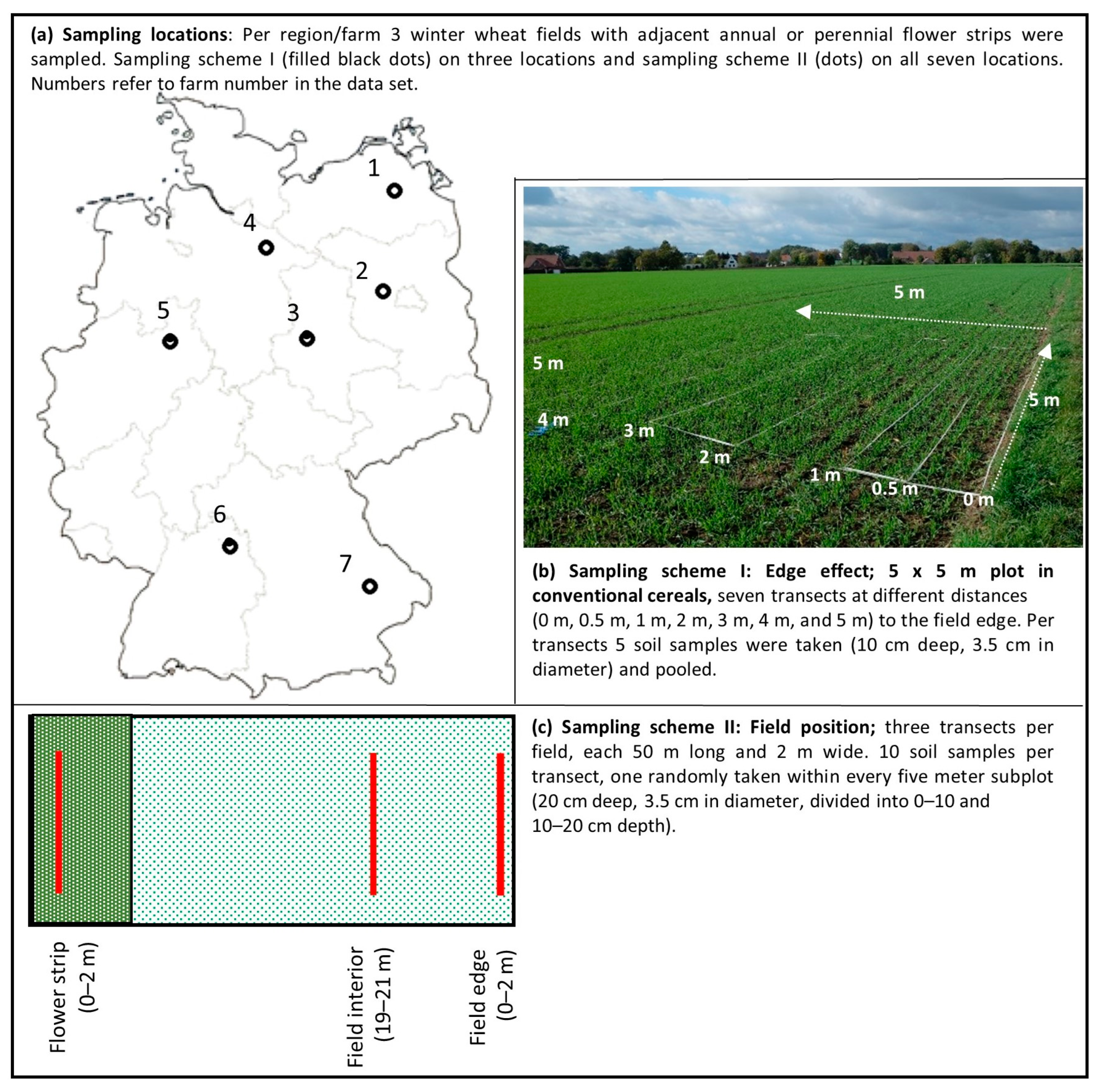
2.1. Locations and Sampling Design

We studied intensively managed agricultural fields in seven different regions of Germany from the Baltic Sea coast to Bavaria and Baden-Württemberg in the south (see Figure 1a). The farms were participating in the F.R.A.N.Z. project (Future Resources, Agriculture, and Nature Conservation;) which pursues a participative approach to increase farmland biodiversity in cooperation with farmers. Agri-environmental measures, established on these conventionally managed farms in different, representative agricultural landscapes of Germany, are monitored with respect to their effect on agrobiodiversity and the costs of implementation. Locations with marginal agricultural yield or known populations of species worthy of protection on farmland are identified, and options of different agri-environmental measures are assessed. In the process, issues such as accessibility, regulations, ownership (e.g., for rented land), or potential weed burden in the soil seed bank are addressed. These issues affect how the emergence of problematic and (from a conservation point of view) desirable weed species are viewed during implementation, as well as afterward, when the area is reintegrated into the normal crop rotation scheme.
All study fields were sown with winter wheat in autumn 2018 and had adjacent flower strips that varied in width (5 to 18 m) and the seed mixture used. The positioning and implementation of agri-environmental measures in the project required certain compromises in order to meet demands in terms of practicability, ecological utility, and statistical requirements. Farms differed in size (seven farms with mean field sizes ranging from 3 to 32 ha; smallest field: 0.1 ha, largest field: 149 ha), soil quality (18–90 soil quality score), tillage regime (low-tillage N = 3, rotational tillage N = 1, and conventional tillage N = 3 farms), and main crops (cereals and maize) cultivated (see Table S1), broadly representing the spectrum of farm types and agricultural landscapes existing in Germany. Soil types in nearby unmanaged land ranged from Gleysols with poor fertility to Cambisols with relatively low to high fertility and Chernozems with very high fertility.
Winter cereals, notably wheat and barley, were cultivated on all farms, followed with lower frequency by maize and root crops such as potato and sugar beet. Low-tillage farms performed no ploughing of arable land, but used disc harrows, drag harrows, spring-tooth harrows, etc. for shallow cultivation and direct drilling in case of intercrops. Conventional tillage, practiced on three farms, implied ploughing and overturning of soil. One farm practiced rotational tillage with ploughing only after or before specific crops (not included in the analysis of tillage effects). Hereafter, diaspores of plants are referred to as seeds, although some are, in fact, fruits. Two sets of seed bank samples were taken to test the hypotheses.

2.2. Sampling Scheme I Edge Effect: Analysis of the Effect of Field Edge

To investigate the gradient in seed density and species number from the field edge to the center of the field, sampling scheme I (Figure 1b) was carried out on three farms (see Figure 1a, black squares), located in Magdeburger Börde (farm 3), Ostwestfalen-Lippe (farm 5), and Hohenlohe (farm 6). On each farm, three freshly sown winter wheat field edges were chosen. All wheat field edges were located next to sealed roads with 0.3 to 2 m wide grassy field margins in between. Square plots of 5 m × 5 m were placed on the field edge with one square side being placed on the outermost furrow of the field. Within the plot, seven parallel transects of 5 m length and 1 or 0.5 m width were demarcated at 0, 0.5, 1, 2, 3, 4, and 5 m distance to the field edge (Figure 1b). Per transect, five soil samples were taken, randomly placed within each meter, using a manual steel cylinder of 10 cm length and 3.5 cm diameter (480 cm3 soil volume). All five soil samples per transect were pooled, resulting in seven analyzed samples per field. A total area of 0.3 m2 (to 0.1 m depth) was sampled.

2.3. Sampling Scheme II Field Position: Seed Bank Enrichment in Flower Strips

For this sampling scheme, we selected 21 winter wheat fields located on seven farms (see Figure 1a). On each farm, we sampled 2–3 fields with adjacent flowering strips in autumn 2018. The flower strips were established in spring 2017 and, thus, had passed their second growing season when sampled (see Figure S1). Some strips were resown in spring 2018 and were prepared during the sampling for re-seeding in spring 2019. Thus, the vegetation in these strips was removed, and soil cultivation in the form of soil-turning ploughing and chisel ploughing had been practiced. We applied a space-for-time approach and paired-sample design to account for differences between fields in terms of management history, climatic conditions, and soil properties. Seed bank sampling was conducted in three 50 m long and 2 m wide transects established in every field: one transect lay at the field edge within a flower strip, another one at a field edge without a flower strip (if possible, with similar neighboring vegetation structure), and a third one in the field interior 20 m distant to the edge (see Figure 1c). Each transect was divided into five subplots of 5 m × 2 m size. In each subplot, one random soil sample was taken with a cylindrical steel probe of 20 cm length and 3.5 cm in diameter. Samples were divided into depths of 0–10 cm and 10–20 cm, and then pooled for every depth within a transect, resulting in two samples per transect (960 cm3). In scheme II, a total soil surface area of 0.6 m2 (to a depth of 0.2 m) was sampled.

2.4. Seedling Emergence Method

After stratification of the samples at 5 °C in darkness in a refrigerator for 2 months, the samples were processed according to the procedure outlined by Ter Braak et al. [32]. Samples were washed through sieves (0.5 mm mesh size for gravel and twigs, and 0.02 mm mesh size for clay, while sand could not be removed); the seed material was spread out on fertilized garden soil and covered with a thin layer of sand on top. Seed germination took place in a greenhouse that was kept at 15 °C during the night and 18 °C during the day (12:12 h dark/light period). Water was added as needed. Seedlings were identified according to images given in Hanf [33] and counted. Unidentified seedlings and type individuals were repotted into separate pots for later identification and confirmation of species according to Jäger and Werner [34]. After no more new seedlings were found to emerge, watering was stopped, and samples were dried out. Six months later, a second germination procedure was started by resuming the watering cycle for an additional 10 weeks. For preparation, the topsoil layer with the samples was disturbed, and the crust was destroyed and turned over. All additionally emerging seedlings were handled in the same manner as in the previous round.
Challenges encountered in the species identification of seedlings led to the following species complexes being defined: Matricaria spp. and Tripleurospermum spp. were summarized as ‘Chamomilla’; Urtica dioica and Urtica urens were classified as ‘Urtica dioica/urens’; Papaver rhoeas, Papaver dubium, and unidentified Papaver spp. were summarized as ‘Papaver spp.’; Amaranthus spp., Epilobium spp., Euphorbia spp., Geranium spp., Juncus spp., Solidago spp., and Taraxacum spp. were not determined to species level. A total of 174 seedlings remained unidentified (as they died during growth cabinet failure) and were categorized as either grass (i.e., graminoids, sedges, or rushes; 165 seedlings) or forb (i.e., non-graminoid herbaceous species; nine seedlings). Woody seedlings referred either to Populus or Betula spp., as both tree species are common within the project area. Populus spp. were also present with two seedlings in the control plots; however, they were not taken into account. Species were classified as forbs or graminoids, and the number of species and seedlings per group was calculated for the different localities and soil depth levels in the field.
Climatic and edaphic site factors at the sampling locations were assessed with Ellenberg indicator values of the plant species recorded [35]. To this end, we calculated abundance-weighted means. The aboveground vegetation in the transects (species composition and cover in percentage classes after Londo) was assessed by relevés recorded in summer 2018 in the 50 m × 2 m plots (for further information on sampling method, see Sutcliffe and Leuschner [36]).

3. Statistical Analysis

To test hypotheses I and II, a subset of seed bank samples collected in scheme II was used, i.e., soil seed bank samples from three low-tillage and three conventional tillage farms. In total, these comprised 17 field edge and associated field interior plots subdivided at different soil depths. We ran linear mixed models using the ‘lmer’ and ‘anova’ functions of the ‘lme4′ (v1.1.31) and ‘lmertest’ (v3.1.3) packages [37,38] in R software [39] version 201.09.1, considering field within farm as random grouping variables, to analyze the number of species (log-transformed) and emerged seedlings (log-transformed) as a function of field location, tillage scheme, and soil depth. Subsequent pairwise comparisons using the ‘emmeans’ function of the ‘emmeans’ (v.1.8.2) package [40] with Tukey p-value correction for multiple testing was used to analyze differences between different soil depths. For all models, fit was evaluated with the ‘simulateResiduals’ and ‘plot’ functions of the ‘DHARMa’ (v0.4.6) package [41]. Furthermore, in sampling scheme I (three farms with three cereal fields each), the number of species and seeds was tested for differences as a function of distance to the field edge, applying the same statistical methods to test hypothesis I. Out of the nine tested fields, one field was removed as an outlier (11 species and 167 seedings on average compared to six species and 20 seedlings per distance class; after consultation with the farmer, the plot was identified as a recent construction site), resulting in eight fields for the final analysis.
To test hypothesis III, 19 fields from seven farms investigated within sampling scheme II, which comprised transects located on field edges with flower strips or on the edge of conventional cereal fields, and in the field interior were taken. Linear mixed models using the ‘lmer’ and ‘anova’ functions, considering field within farm as a random grouping variable, were run to analyze the number of species (log-transformed) and emerged seedlings per m2 (log-transformed) as a function of the field location. Subsequent pairwise comparisons using the ‘emmeans’ function with Tukey p-value correction for multiple testing were conducted. The analysis was performed with all species and subsequently with the species added by the flower seed mixture excluded.
Furthermore, differences in the species composition of field edge, interior, and flower strip were analyzed employing NMDS (nonmetric multidimensional scaling [42]) using the ‘metaMDS’ function from the ‘vegan’ (v2.6.4) package [43] based on Bray–Curtis distances. Very abundant species were down-weighted using the Hellinger transformation [44]. Effects of farm and field location were first checked by correlation analysis using the ‘envfit’ function from the ‘vegan’ package, and then analyzed by pairwise PERMANOVA analysis, with Bonferroni-corrected p-values. We checked for differences in between-plot variation (beta diversity) by employing the ‘betadisper’ function from the ‘vegan’ package. The calculated weighted mean Ellenberg indicator values were plotted for each transect to inform about environmental conditions at the sampling site. Missing or indifferent values were substituted by average values specific for the field location. Testing of significance was performed with the ‘envfit_cwm’ function from the ‘weimea’ package version 0.1.4, accounting for species abundance, and eliminating highly significant correlation values due to circular reasoning [45]. We tested for autocorrelation between individual indicator values using the ‘cor.mtest’ function from the package ‘corrplot’ (v0.92) [46]. As the last step, the ‘multipatt’ function from the ‘indicspecies’ package (v1.7.12) [47] was used to identify species associated with flower strips, field edges, or the interior.
Comparisons between aboveground vegetation and seed bank (hypothesis IV) were conducted on the basis of species presence/absence data. First, the Sørensen index was calculated for every plot pair/transect (seed bank vs. flower strip). Second, the species composition was analyzed by performing an NMDS, using the ‘metaMDS’ function in R. Only species occurring in more than three transects were considered. On five transects, no non-crop species and, on a further four transects, only one non-crop species were found in the aboveground vegetation. Those transects were all located in the field interiors; therefore, we excluded all field interior transects from this analysis, resulting in 19 transects on flower strips and field edges, respectively. For better comparability, some plant species present in the aboveground vegetation were summed up in species complexes as were used in the seed bank analysis (e.g., Silene spp. and Poa spp.). Furthermore, tree species such as Acer campestre and Alnus glutinosa were removed. The effects of field location (flower strip vs. field edge) and data type (seed bank vs. aboveground vegetation) were tested with the ‘envfit’ function.
Data were analyzed with R software [39]. Graphs were generated using the ‘ggplot2′ (v3.4.0) package [48] and ‘ggrepel’ (v0.9.2) [49].

4. Results

In the 252 soil samples, a total of 10,828 seeds germinated and could be identified to species (118) or genus (14) level. The number of species per 50 m transect sample varied between two (field interior) and 35 (flower strip), while the number of seedlings varied between three and 557, respectively. The extrapolated number of seeds expected to be present in the seed bank of 1 m2 of the studied arable land varied between 6000 and 12,000 (flower strips on average: ~29,800, field edges: ~12,100, and field interior: ~6000).

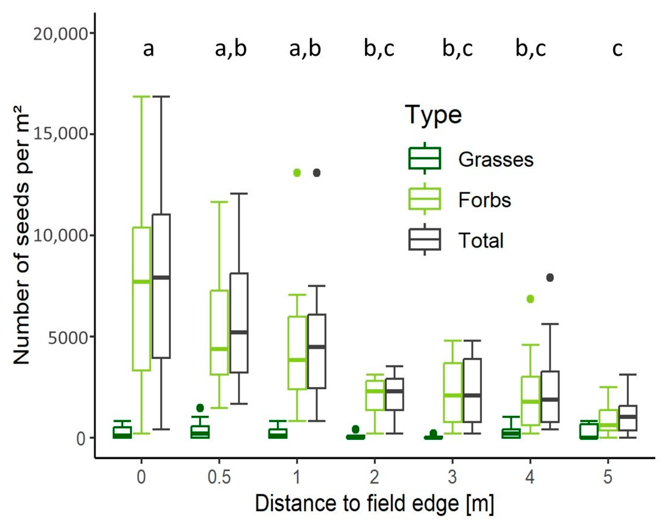
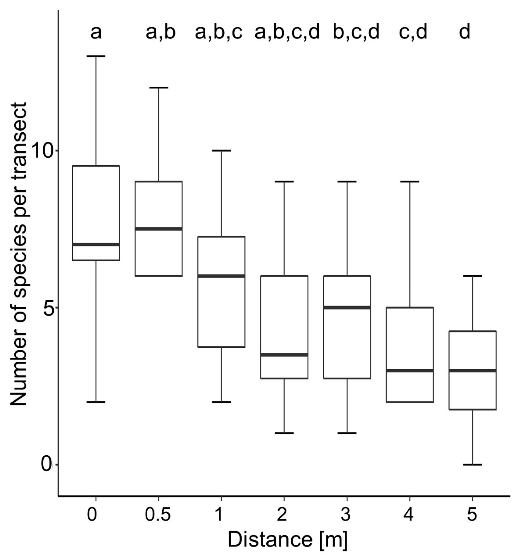
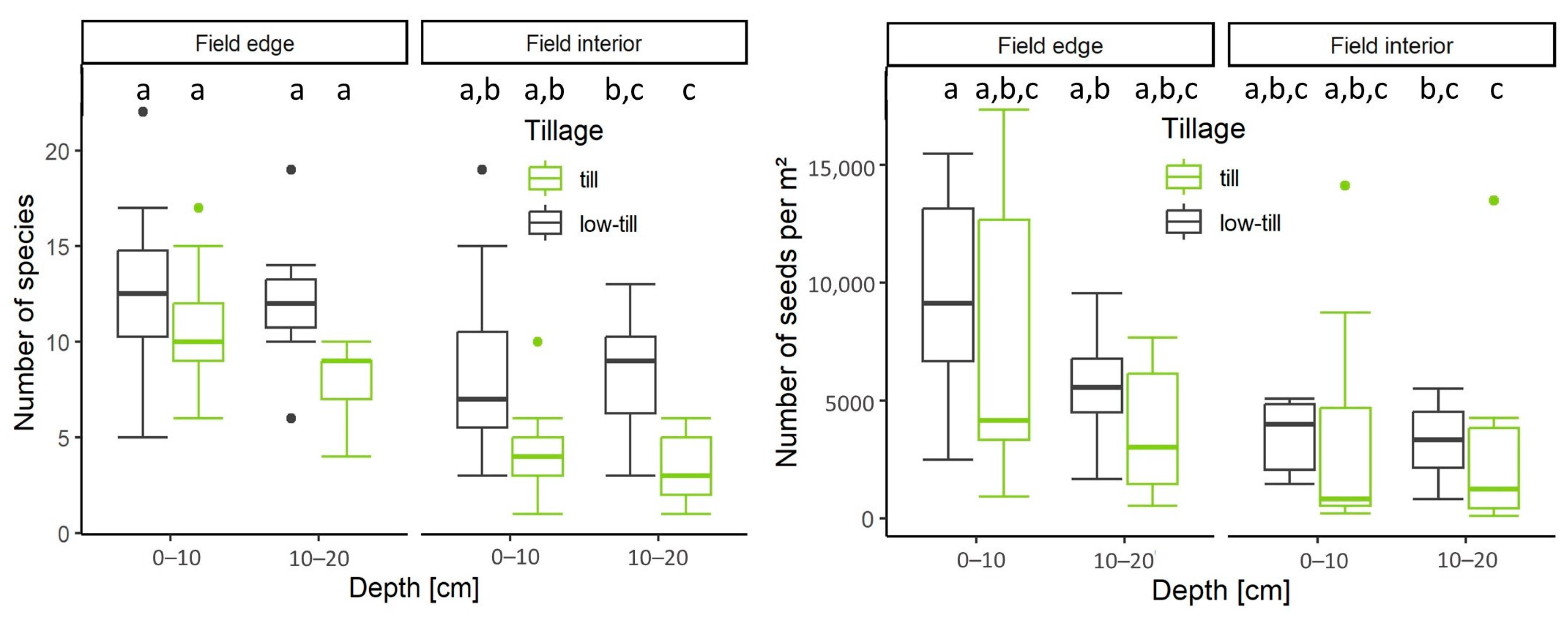
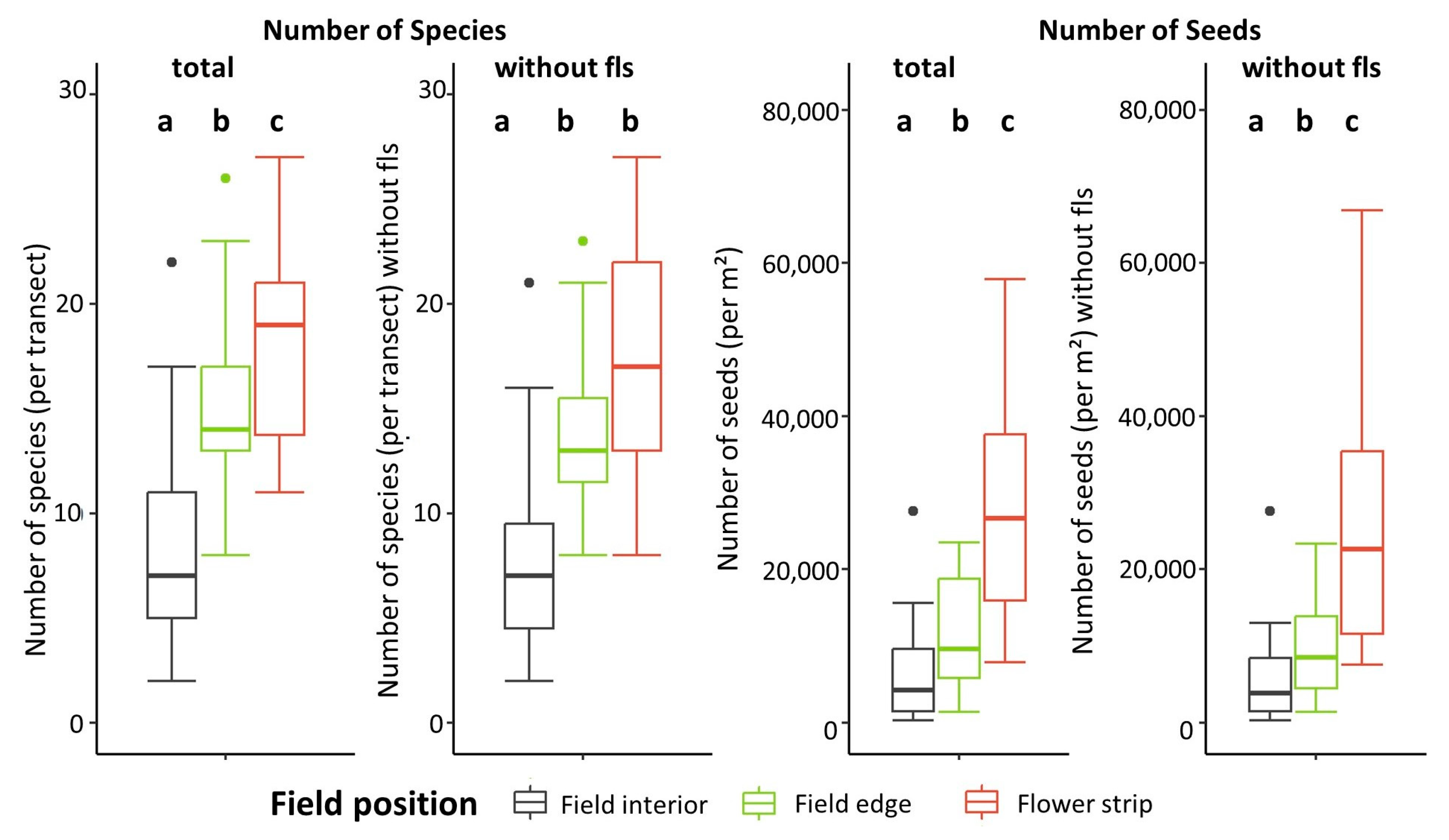
4.1. Number of Species and Seeds in Relation to Tillage Regime, Soil Depth, and Distance to Field Edge

Within the seed bank sampling scheme I ‘edge effect’, a total of 1276 seedlings were counted and assigned to 58 species/groups (see Table S2). Chenopodium album accounted for around 40% of all seeds, followed by Urtica dioica/urens with 10% of the germinated seedlings. Fifteen species were present only once (e.g., Anagallis arvensis, Linaria vulgaris, and Sagina procumbens), while an additional 18 species were present between two and five times (e.g., Mercurialis annua, Galium aparine, and Veronica hederifolia). On average, one out of the nine present grass species was observed in the subplots of varying distance with, on average, only one individual. The transect analysis in the 5 m × 5 m plots showed a significant decrease in species numbers and seed numbers within 1 m from the edge (Figure 2). Forb species decreased with increasing distance to the edge from around seven to two species and from 8000 seedlings to 1000. The number of seeds decreased from around 40 at 0–1 m to 10 seeds between 2 and 5 m (mixed model: sum of squares = 18.8, F6,39 = 8.8, p < 0.0001). Five times more seedlings were present next to the field edge in the outermost subplot (0–0.5 m) than at the 5 m distance (0–5 m), and almost four times more seedlings were present at 0.5 m compared to the 2 to 5 m distance.
With increasing distance to the field edge, the number of species in the seed bank significantly decreased (Figure 3; mixed model: sum of squares = 3.4, F6,35 = 6.9, p < 0.0001). On average, seven species occurred in the seed bank between 0 and 1 m distance, and four species occurred between 2 and 5 m distance.
Tillage regime and location (edge vs. field interior) both had a significant effect on the number of seeds and species present in the seed bank (Figure 4 and Table 1). In general, the number of seeds and species present was significantly higher at the field edge compared to the field interior (Table 2). The number of species and the number of total seeds did not significantly differ according to soil depth.
Around two-thirds of seeds and species were found in the uppermost 10 cm of soil (mean number ± standard error of seeds per m2 on average: 6048 ± 800, species 9 ± 1) and one-third at 10–20 cm depth (seeds: 3844 ± 524, species 8 ± 1). We found significantly more seeds in low-tillage fields (mean of field interior: 7598 ± 1533, field edge: 15,078 ± 2236) than under conventional tillage (field interior: 6419 ± 2996, field edge: 10,794 ± 2749).
The number of species was also significantly higher in low-tillage fields (field interior: 8 ± 1, field edge: 12 ± 1) than at conventional tillage (Figure 4 field interior: 4 ± 1, field edge: 9 ± 1).

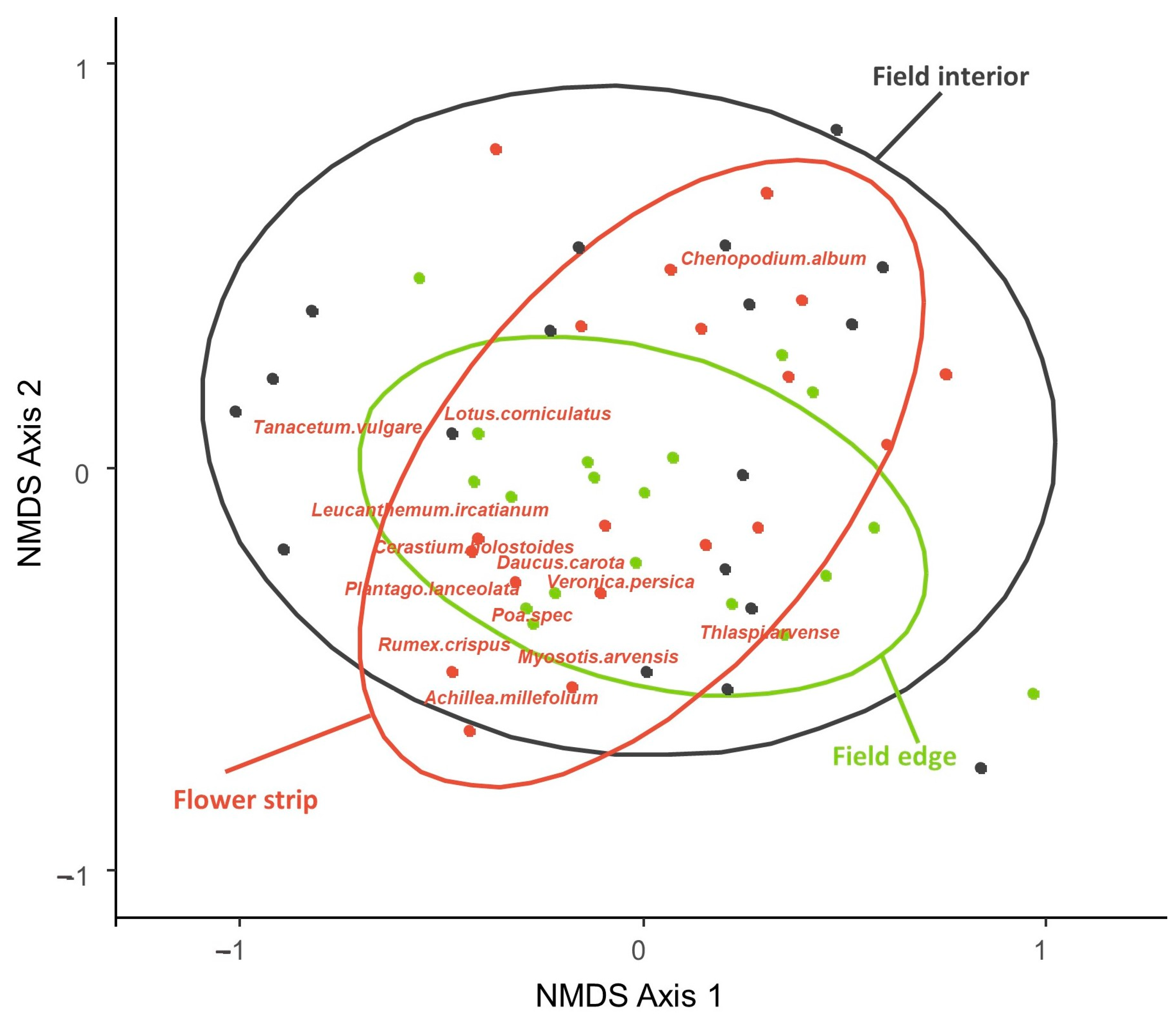
4.2. Differences in Abundance, Species Numbers, and Species Composition of the Seed Bank According to Field Location

In total, 8786 seedlings were counted (flower strip: 5445; field edge: 2166; field interior: 1175) in sampling scheme II and assigned to 113 species/groups (see Table S3). Overall, 85% of the seeds were forbs, and 15% were grasses (158 seedlings remained unidentified), with proportionally more gramineous seedlings observed in field edges (80:19) and interiors (83:15) than in flower strips (88:11).
Comparing the species composition of the seed bank of flower strips, field edges, and field interiors revealed no significant differences among the three habitat types, when taking the abundances of the 113 species/groups into account. A total of 41 species occurred in all three field locations. The most abundant species, i.e., Chenopodium album, Urtica spp., and species of the ‘Chamomilla’ group, were also found on most transects.
Transects located in the north/northeast of Germany with low tillage and rotational tillage were concentrated in the upper part of the NMDS plot, while transects from farms in southern and southwestern Germany with conventional tillage dominated in the lower part (Figure 5). The NMDS further revealed that field location did not correlate with either of the axes but that the factor farm strongly correlated with the first axis (R2 = 0.40, p = 0.001). None of the Ellenberg indicator values were significantly correlated with the NMDS axes (results not shown).
The number of species and seeds in the seed bank differed significantly across the three field locations (see ANOVA results of fixed effects in Table 2 and Figure 6).
The number of seeds per m2 was highest in the flower strips, irrespective of whether the sown species in the flower strips were included (mean ± s.e.: 29,633 ± 4369), followed by field edges (11,801 ± 1632) and field interior (6420 ± 1565). The number of species, including sown species, was significantly higher in flower strips (19 ± 2) than at the field edges (13 ± 1). When excluding the sown species, the number of species in the seed bank was equal in flower strips and field edges (12 ± 1 and 11 ± 1), but still significantly higher than in the field interior (6 ± 4).

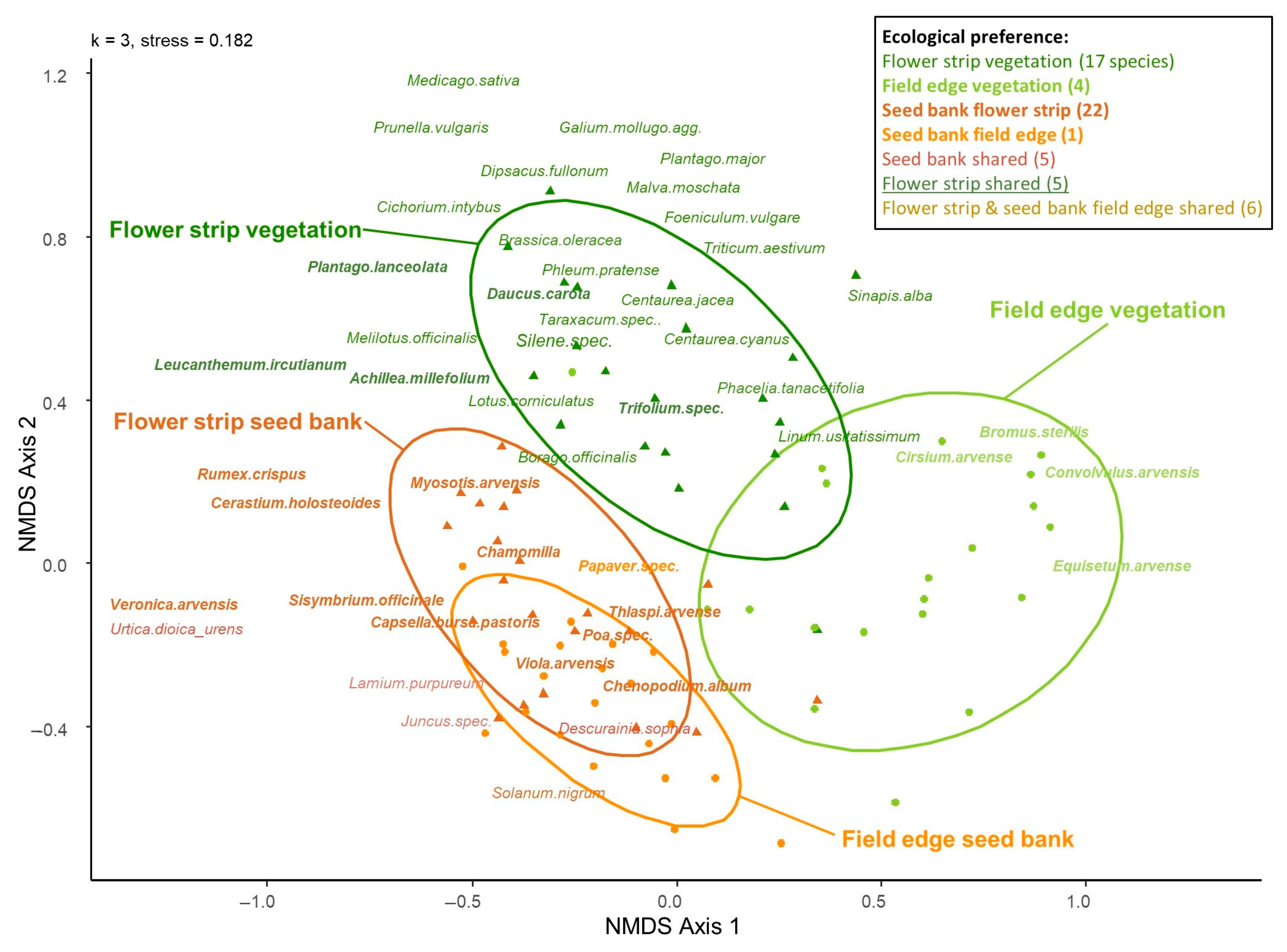
4.3. Differences in the Composition of Seed Banks and Associated Above-Ground Vegetation

We found 114 species/species complexes in the seed bank, while 176 species were present in the aboveground vegetation of the plots. A total of 71 species were shared between seed bank and vegetation, including the abundant annuals Chenopodium album and the ‘Chamomilla’ group. A total of 43 species were only present in the seed bank (e.g., Juncus spp. and Lamium purpureum), while 105 taxa occurred exclusively in the aboveground vegetation (e.g., Dipsacus fullonum, see summary in Table S3). The NDMS revealed significant differences in species composition between field edge and flower strip on the one hand, and between seed bank and aboveground vegetation on the other (Figure 7). Both habitats (flower strip vs. field edge: envfit analysis R2 = 0.19, p = 0.001) and vegetation components (seed bank vs. vegetation: R2 = 0.38, p = 0.001) were significantly correlated with the two first NMDS axes.
According to the multipattern analysis (for details, see Table S5), 25 out of the 27 species associated with flower strips originated from the seed mixture, of which five were also associated with the soil seed bank and 17 were identified as weeds. While the number of species associated with the field edge is low, no associated species were shared between the vegetation and the soil seed bank.
Furthermore, the multi-pattern analysis showed that many species contained in the flower strip seed mixtures were significantly correlated to the above-ground vegetation (e.g., Foeniculum vulgare and Silene spp.), while non-sown weed species of the aboveground vegetation, i.e., spontaneously occurring taxa, were more often correlated to the seed bank in flower strips and field edges (e.g., Juncus spp., Chenopodium album, and Capsella bursa-pastoris). Some flower strip species were common in the seed bank and the aboveground vegetation (e.g., Leucanthemum vulgare/ircutianum, Daucus carota, and Achillea millefolium). Common in the aboveground vegetation but absent from the seed bank was, for example, Cirsium arvense.
The number of species was higher in the aboveground vegetation than in the seed bank in flower strips (seed bank vs. vegetation; 18 vs.25), but higher in the seed bank at the field edges (13:8) and in the field interior (7:3). A similar pattern was observed for plant abundance (seed numbers and vegetation cover). When expressed in relative values (flower strip set to 100%), species numbers in the aboveground vegetation decreased from 10% in the field edge to 3% in the field interior, while the number of seeds dropped to 41% and 20% compared to the flower strips. The Sørensen similarity index indicated the highest similarity of vegetation and seedbank in flower strips, followed by field edges and by field interiors (Table 3).

5. Discussion

In this comparative study of the seed bank in flower strips, field edges, and field interiors in intensively used agricultural landscapes in seven regions of Germany, the extrapolated number of seeds varied between 6000 and 12,000 per m2 of arable land. While these numbers are lower than seed densities of 47,000 per m2 reported from sandy fields in eastern Poland [50], up to 20,000 per m2 from Danish fields [51], and of 15,000 per m2 from Czech fields [52], seed densities in our study matched very well seed densities from Poland [53], southern Germany (8270 per m2 [54]), and northern Germany (approximately 8500 per m2 [17]).

5.1. Edge Effect and Low-Tillage Increase Seed Bank Density in Arable Soils

Confirming our first hypothesis, we found more species and higher total seed numbers in field edges compared to the field interior. Sampling in small distance steps from the edge confirmed that a pronounced edge effect does exist within the first 2 m of the field. This result is in accordance with several other studies from Europe, confirming that field edges can be refugia for various weed species, including rare taxa, while the field interior is much less diverse [7,23,55]. A study on the arable seed bank of dicotyledons in England found mostly arable weeds within the first few meters, while species originating from the margin vegetation, such as Galium aparine and Urtica dioica, were rather rare in that soil seed bank [22]. In line with our results, the same study revealed a decrease in seed bank diversity and density within the first few meters. Interestingly, in our study, the reduction in seed and species numbers from field edge to interior only occurred in forbs, while grasses stayed constant with on average one species and one seed per m2 along the same gradient. The low density of grass seeds is unexpected, because we anticipated seed rain from the adjacent grassy field margins at least within 1 m of the field. One possible explanation could be the maintenance regime of the field margins, the regular cutting of which prevents successful seed production (own observation and personal communication of the farmers). In addition, seed rain from the field margins might be limited due to the very narrow field margins in our study (less than 0.5 m wide).
Our second hypothesis prediction that fields on low-tillage farms contain more seeds and species in the seed bank than fields under conventional tillage was also confirmed by our data. However, contrary to our expectations, we did not find a significant decrease in the number of seeds with increasing soil depth, i.e., from 0–10 cm to 10–20 cm, in any habitat type. This might have been caused by the fact that even low-tillage regimes disturb the topsoil layer to a depth of up to 20 cm, depending on the equipment used. Therefore, seeds will be evenly distributed within the top 20 cm, independent of the tillage system. A study on the effects of different tillage systems on the vertical distribution of seeds at three sites in England also found no vertical differences in seed numbers for conventional and low-tillage systems. In fact, accumulation of seeds in the first 5 cm of the topsoil was found only in zero-tillage systems [56]. In general, the size of the seed bank increases with conversion from conventional tillage to low-tillage systems. However, there are complex interactions of tillage system, herbicide application, and crop rotation (reviewed in [57]). Low and no tillage, combined with specific crop rotations and pesticide application schemes, might even lead to a decrease in weeds in the soil seed bank, when mechanical weed control is replaced by intensified chemical control [58,59].
In our sample of seven farms, geographical location, soil properties, and local differences in crop rotation must be taken into account as additional explanatory variables when explaining seed bank differences. This is reflected in the fact that all large farms in our sample were located in the north and northeast of Germany and were practicing low tillage, while the smaller, family-run farms characteristic for western and southern Germany carried on with conventional tillage. Taking further into account that species pools usually differed across regions [3,60], our finding that the variable ‘farm’ explained more variation in species composition than habitat type (or field location) seems to be the result of a complex interplay of these factors. Consequently, only 12 of 117 plant species occurred in the seed bank of all seven farms that were studied. The ubiquitous species included taxa such as Chenopodium album, the Chamomilla group, and Poa spp. However, all three taxa exhibit large differences in seed density between farms. This result is consistent with findings of a comparable study on weed species in the aboveground vegetation of fields located in Catalonia (Spain) and Lower Saxony (Germany), where a share of common species of only 15% was reported [61]. A study in Bavaria identified management factors, notably previous crop cover, as one of the most important factors influencing the density and composition of the seed bank [28]. In our study, the seed bank of directly neighboring fields within one farm also showed high small-scale variation.
Certainly, a more comprehensive analysis with consideration of the complexity of the surrounding landscapes [62], as well as crop rotation patterns, might help to explain differences between farms and to quantify the effect of geography on seed bank composition. Yet, despite considerable variation among fields due to crop rotation, soil type, and herbicide and fertilizer use patterns, our data show a negative effect of conventional tillage systems on seed density compared to low- or no-tillage systems.

5.2. Flower Strips Enrich the Quality and Quantity of Seed Banks

In line with our third hypothesis, seed banks of flower strips had higher species numbers and seed densities than adjacent fields both at the field edge and in the field interior. We found 2–3 times higher seed densities on flower strips than on field edges in equivalent positions, regardless of whether sown flower strip species were included or not. Yet, the total number of species found in the seed bank of flower strips was not elevated in comparison to the field edges, indicating that sown species seemed not to accumulate in the soil seed bank, at least within the first 2 years after sowing. The seed bank composition supports this finding, i.e., we observed a similar arable species composition in the seed bank of flower strips and conventional field edges after two vegetation periods. However, some species such as Chenopodium album, Veronica persica, Thlaspi arvense, and Rumex crispus were found to be associated with flower strips and, thus, seem to have benefited from their establishment. It is well known that these taxa can reach high densities in the seed bank due to a high seed production per plant [63,64,65]. T. arvense, for example, can shed up to 3000 and R. crispus can even shed up to 60,000 seeds per plant. Both species may also profit from the lack of pesticide application in flower strips and are, therefore, able to replenish their seed bank. Nevertheless, this did not lead to a principal difference in species composition between flower strips and field interior. If at all, we expect this differentiation to occur only several years after flower strip establishment.
In line with this finding, only a few species from the sown seed mixture, e.g., Plantago lanceolata or Daucus carota, were able to establish a seed bank. Possible causes for this might be the short lifespan of the flower strips due to flower strip management by farmers, which may have prevented the development of adult seed-producing individuals of perennial plant species. In contrast, studies on vegetation development of undisturbed flower strips with high sown wild plant diversity show that these plants are able to establish a seed bank and make reseeding superfluous [66].
We expected that higher fertilizer load and, as a result, lower light availability in the field interior compared to field edges would translate into marked differences in Ellenberg indicator values. However, no such pattern was found. Similarly, in arable fields in northeastern France, aboveground vegetation of field edges and field interiors did not differ in Ellenberg nitrogen and light values, which led the authors to the conclusion that field edges and interiors have similarly high nutrient levels [23]. Newly established flower strips did not change that matter.
Concerning the accumulation of problematic weed species in the seed bank, we observed a significant increase in some problematic species, i.e., Chenopodium album, Rumex crispus, Poa spp., and Echinochloa crus-galli. Consequently, we observed increasing application of herbicides in the course of flower strip establishment, a phenomenon that was especially pronounced on low-tillage farms. Some farmers even decided against re-establishment of flower strips, terminated agri-environmental measures ahead of time, and re-established crop fields on the area of flower strips to suppress emerging weeds. In addition, those areas were often treated with higher amounts of herbicides to combat and prevent the spread of occurring weeds (personal communication of local farmers). Since this development calls into question the whole point of flower strip establishment, advice to farmers must improve to reduce the risk of weed infestation after the establishment of flower strips. Adapting the seed mixtures and cutting the vegetation at 25–30 cm height in the first year could help to overcome some of the problems associated with flower strip establishment [67].
The composition of the aboveground weed vegetation of conventionally managed fields made it unlikely that high-nature-value species or taxa not present in the aboveground vegetation can be still found in the seed bank [25]. In general, seed banks of farmland with a long history of intensive use, i.e., high chemical and physical stress levels, are mostly depleted [68]. As a consequence, the restoration potential of the seed bank is limited [29]. Despite the limitations of seed bank analyses to detect rare species, we found two individuals of Myosurus minimus, a species classified as vulnerable according to the red list of threatened plants [69].
Our study of seed bank changes in the context of short-term establishment of flower strips on fertile arable land shows that only few and common sown flower strip species, such as Plantago lanceolata or Daucus carota, were able to establish also in the seed bank after two vegetation periods. We found no general increase in seed bank diversity under flower strips, but observed an increase in some problematic weed species, which might have jeopardized the acceptance of agri-environmental measures by farmers.

5.3. Larger Differences between Aboveground Vegetation and Seed Bank in the Field than in Flower Strips

Comparison of seed bank and aboveground vegetation in the three field locations revealed a higher Sørensen similarity index for flower strips compared to field edges and field interior. A study comparing seed bank and aboveground vegetation before first herbicide application on seven spring barley fields in England found that, depending on the species, 0.4–55% of the seeds were present as seedlings in the aboveground vegetation. This highly variable relation is largely influenced by the coincidence of crop management schemes and the timing of seedling emergence [22]. The aboveground vegetation in the field interior often comprises only the cultivated crop and barely any additional weed species, while the soil seed bank may still contain some additional species. Under intensive conventional farming practices, most weed seedlings in the field will not fully develop as a consequence of herbicide use and low light availability under the crop [26], while the seed bank often is less impacted by the management regime [70,71], which can explain low similarity between aboveground vegetation and seed bank. At the field edge, where fertilizer and pesticide amounts are usually reduced, more weed species are typically able to establish themselves as plants [5]. In flower strips, with reduced to no fertilization and use of herbicides, similarity between seed bank and aboveground vegetation was highest, although many sown species were missing in the seed bank. The high similarity in flower strips is confirmed by another study investigating the established flora in sown flower strips [72]. They found that over half of species present in the vegetation were not sown. Among the most abundant plants were several common weed species, probably germinated from the seed bank. The spatial distribution of seeds in the soil is usually highly patchy [21]. In arable fields, however, regular soil disturbance may lead to a more even distribution pattern of the seed bank, which may also translate into a more evenly distributed aboveground vegetation. Consequently, when no herbicides are applied, Sørensen’s similarity index between vegetation and seed bank may reach values as high as 65% [73].

6. Conclusions

In this study, we showed that the weed seed banks in conventional arable fields of seven regions of Germany were, apart from a few dominant species, largely depleted. However, species diversity and the abundance of seeds were still higher at the field edge, which may provide refugia for some arable species. Low-tillage regimes in general seemed to support higher seed densities and a greater number of species in the seed bank in the upper 20 cm of soil than conventional tillage. Regardless of tillage system, the seed bank was found to be largely dominated by nitrogen- and light-demanding competitive species. Flower strips of short duration, a widely established element of agri-environmental measures to increase biodiversity in intensive farmland, only showed a limited potential to enrich the depleted seed bank with naturally occurring or even rare arable species. The possible increase and dominance of problematic weed species on flower strips needs close monitoring, especially on fertile soil. Otherwise, increased herbicide treatment to control weed-dominated flower strips may outweigh any positive conservation benefit of flower strips.

Supplementary Materials

The following supporting information can be downloaded at: https://www.mdpi.com/article/10.3390/land12040926/s1, Figure S1: Soil seed bank sampling; (a) field edge with winter cereals, (b) flower strip in autumn, (c) soil sampling and (d) seedling emergence in the green house. Table S1: Mean field size [min:max], soil quality score (SQR), tillage regime and main crops cultivated on the 7 studied farms. Table S2: Species list for distance classes (alphabetically ordered), mean values for species and seed [mean ± sd] and total number of seedlings per species. Table S3: Species list of sampling scheme II, field position, with total number of seedlings per transect (sampled area 0.01 m²) and number of transects. Table S4: Results of multilevel pattern analysis, only significant species associations are shown. Table S5: Results of multilevel pattern analysis, only significant species associations are shown.

Author Contributions

Conceptualization, L.S. and T.W.D.; methodology, L.S. and T.W.D.; software, L.S.; validation, L.S. and L.M.E.S.; formal analysis, L.S.; investigation, L.S. and L.M.E.S.; resources, C.L.; data curation, L.S.; writing—original draft preparation, L.S.; writing—review and editing, L.S., L.M.E.S., C.L. and T.W.D.; visualization, L.S.; supervision, T.W.D. and C.L.; project administration, L.M.E.S.; funding acquisition, C.L. All authors have read and agreed to the published version of the manuscript.

Funding

This research was funded by the Federal Ministry of Food and Agriculture, Federal Office for Agriculture and Food (grant number 817760), as well as by the Federal Agency for Nature Conversation (grant number 3516880500), with funds from the Federal Ministry for the Environment, Nature Conversation, Building, and Nuclear Safety.

Institutional Review Board Statement

Not applicable.

Informed Consent Statement

Not applicable.

Data Availability Statement

Data are available in a publicly accessible repository. The data presented in this study are openly available from the Open Science Framework (OSF) at DOI 10.17605/OSF.IO/YNQR3.

Acknowledgments

The authors gratefully acknowledge the cooperation of the participating farmers. Appreciation also goes to their colleagues and friends, especially Regina Helbig and Joachim Schnee, who assisted in collecting, preparing, and taking care of the soil seed bank samples.

Conflicts of Interest

The authors declare no conflict of interest.

References

  1. Rollin, O.; Benelli, G.; Benvenuti, S.; Decourtye, A.; Wratten, S.D.; Canale, A.; Dexneus, N. Weed-insect pollinator networks as bio-indicators of ecological sustainability in agriculture. A review. Agron. Sustain. Dev. 2016, 36, 8. [Google Scholar] [CrossRef]
  2. Zerbe, S. Species-Rich Arable Land. In Restoration of Ecosystems–Bridging Nature and Humans: A Transdisciplinary Approach; Springer: Berlin/Heidelberg, Germany, 2023; pp. 393–407. [Google Scholar]
  3. Leuschner, C.; Ellenberg, H. Ecology of Central European Non-Forest Vegetation: Coastal to Alpine, Natural to Man-Made Habitats: Vegetation Ecology of Central Europe, Volume II.; Springer: Cham, Switzerland, 2017. [Google Scholar]
  4. Richner, N.; Holderegger, R.; Linder, H.P.; Walter, T. Reviewing change in the arable flora of Europe: A meta-analysis. Weed Res. 2015, 55, 1–13. [Google Scholar] [CrossRef]
  5. Meyer, S.; Wesche, K.; Krause, B.; Leuschner, C. Dramatic losses of specialist arable plants in Central Germany since the 1950s/60s—A cross-regional analysis. Divers. Distrib. 2013, 19, 1175–1187. [Google Scholar] [CrossRef]
  6. Fischer, A.; Milberg, P. Effects on the flora of extensified use of field margins. Swed. J. Agric. Res. 1997, 27, 105–112. [Google Scholar]
  7. Wietzke, A.; Albert, K.; Bergmeier, E.; Sutcliffe, L.M.E.; van Waveren, C.-S.; Leuschner, C. Flower strips, conservation field margins and fallows promote the arable flora in intensively farmed landscapes: Results of a 4-year study. Agric. Ecosyst. Environ. 2020, 304, 107142. [Google Scholar] [CrossRef]
  8. Hoffmann, H.; Peter, F.; Herrmann, J.D.; Donath, T.W.; Diekoetter, T. Benefits of wildflower areas as overwintering habitats for ground-dwelling arthropods depend on landscape structural complexity. Agric. Ecosyst. Environ. 2021, 314, 107421. [Google Scholar] [CrossRef]
  9. Barreiro-Hurlé, J.; Espinosa-Goded, M.; Dupraz, P. Does intensity of change matter? Factors affecting adoption of agri-environmental schemes in Spain. J. Environ. Plan. Manag. 2010, 53, 891–905. [Google Scholar] [CrossRef]
  10. Joormann, I.; Schmidt, T. F.R.A.N.Z.-Studie—Hinternisse und Perspektiven für mehr Biodiversität in der Agrarlandschaft: Thünen Working Paper 75; Thünen-Institut: Braunschweig, Germany, 2017. [Google Scholar]
  11. Espinosa-Goded, M.; Barreiro-Hurlé, J.; Ruto, E. What do farmers want from agri-environmental scheme design? A choice experiment approach. J. Agric. Econ. 2010, 61, 259–273. [Google Scholar] [CrossRef]
  12. Kleijn, D.; Baquero, R.A.; Clough, Y.; Díaz, M.; de Esteban, J.; Fernández, F.; Gabriel, D.; Herzog, F.; Holzschuh, A.; Jöhl, R.; et al. Mixed biodiversity benefits of agri-environment schemes in five European countries. Ecol. Lett. 2006, 9, 243–254. [Google Scholar] [CrossRef]
  13. Melander, B.; Munier-Jolain, N.; Charles, R.; Wirth, J.; Schwarz, J.; van der Weide, R.; Bonin, L.; Jensen, P.K.; Kudsk, P. European perspectives on the adoption of nonchemical weed management in reduced-tillage systems for arable crops. Weed Technol. 2013, 27, 231–240. [Google Scholar] [CrossRef]
  14. Albrecht, H.; Auerswald, K. Seed traits in arable weed seed banks and their relationship to land-use changes. Basic Appl. Ecol. 2009, 10, 516–524. [Google Scholar] [CrossRef]
  15. Thompson, K.; Bakker, J.P.; Bekker, R.M.; Hodgson, J.G. Ecological correlates of seed persistence in soil in the north-west European flora. J. Ecol. 1998, 86, 163–169. [Google Scholar] [CrossRef]
  16. Lang, M.; Prestele, J.; Wiesinger, K.; Kollmann, J.; Albrecht, H. Reintroduction of rare arable plants: Seed production, soil seed banks, and dispersal 3 years after sowing. Restor. Ecol. 2018, 26, S170–S178. [Google Scholar] [CrossRef]
  17. Görzen, E.; Diekötter, T.; Meyerink, M.; Kretzschmar, H.; Donath, T.W. The Potential to Save Agrestal Plant Species in an Intensively Managed Agricultural Landscape through Organic Farming—A Case Study from Northern Germany. Land 2021, 10, 219. [Google Scholar] [CrossRef]
  18. Armengot, L.; Blanco-Moreno, J.M.; Bàrberi, P.; Bocci, G.; Carlesi, S.; Aendekerk, R.; Berner, A.; Celette, F.; Grosse, M.; Huiting, H.; et al. Tillage as a driver of change in weed communities: A functional perspective. Agric. Ecosyst. Environ. 2016, 222, 276–285. [Google Scholar] [CrossRef]
  19. Derpsch, R. Conservation Tillage, No-Tillage and Related Technologies. In Conservation Agriculture; Springer: Berlin/Heidelberg, Germany, 2003; pp. 181–190. [Google Scholar]
  20. Ghersa, C.M.; Martınez-Ghersa, M.A. Ecological correlates of weed seed size and persistence in the soil under different tilling systems: Implications for weed management. Field Crops Res. 2000, 67, 141–148. [Google Scholar] [CrossRef]
  21. Burmeier, S.; Eckstein, R.L.; Donath, T.W.; Otte, A. Plant pattern development during early post-restoration succession in Grasslands—A case study of Arabis nemorensis. Restor. Ecol. 2011, 19, 648–659. [Google Scholar] [CrossRef]
  22. Wilson, P.J.; Aebischer, N.J. The distribution of dicotyledonous arable weeds in relation to distance from the field edge. J. Appl. Ecol. 1995, 32, 295–310. [Google Scholar] [CrossRef]
  23. Fried, G.; Petit, S.; Dessaint, F.; Reboud, X. Arable weed decline in Northern France: Crop edges as refugia for weed conservation? Biol. Conserv. 2009, 142, 238–243. [Google Scholar] [CrossRef]
  24. Yvoz, S.; Cordeau, S.; Zuccolo, C.; Petit, S. Crop type and within-field location as sources of intraspecific variations in the phenology and the production of floral and fruit resources by weeds. Agric. Ecosyst. Environ. 2020, 302, 107082. [Google Scholar] [CrossRef]
  25. Simmering, D.; Waldhardt, R.; Otte, A. Erfassung und Analyse der Pflanzenartenvielfalt in der “Normallandschaft”—Ein Beispiel aus Mittelhessen. Ber. Reinhard-Tüxen-Ges. 2013, 25, 73–94. [Google Scholar]
  26. Kleijn, D.; van der Voort, L.A.C. Conservation headlands for rare arable weeds: The effects of fertilizer application and light penetration on plant growth. Biol. Conserv. 1997, 81, 57–67. [Google Scholar] [CrossRef]
  27. Devlaeminck, R.; Bossuyt, B.; Hermy, M. Inflow of seeds through the forest edge: Evidence from seed bank and vegetation patterns. Plant Ecol. 2005, 176, 1–17. [Google Scholar] [CrossRef]
  28. Albrecht, H.; Pilgram, M. The weed seed bank of soils in a landscape segment in southern Bavaria–II. Relation to environmental variables and to the surface vegetation. Plant Ecol. 1997, 131, 31–43. [Google Scholar] [CrossRef]
  29. Bossuyt, B.; Honnay, O. Can the seed bank be used for ecological restoration? An overview of seed bank characteristics in European communities. J. Veg. Sci. 2008, 19, 875–884. [Google Scholar] [CrossRef]
  30. Hopfensperger, K.N. A review of similarity between seed bank and standing vegetation across ecosystems. Oikos 2007, 116, 1438–1448. [Google Scholar] [CrossRef]
  31. Lang, M.; Kollmann, J.; Prestele, J.; Wiesinger, K.; Albrecht, H. Reintroduction of rare arable plants in extensively managed fields: Effects of crop type, sowing density and soil tillage. Agric. Ecosyst. Environ. 2021, 306, 107187. [Google Scholar] [CrossRef]
  32. Ter Heerdt, G.N.; Verweij, G.L.; Bekker, R.M.; Bakker, J.P. An improved method for seed-bank analysis: Seedling emergence after removing the soil by sieving. Funct. Ecol. 1996, 10, 144–151. [Google Scholar] [CrossRef]
  33. Hanf, M. Ackerunkräuter Europas mit Ihren Keimlingen und Samen, 2nd ed.; BLV Verlagsgesellschaft: Frankfrut, Germany, 1984. [Google Scholar]
  34. Jäger, E.J.; Werner, K. Rothmaler-Exkursionsflora von Deutschland; Springer: Berlin/Heidelberg, Germany, 2011. [Google Scholar]
  35. Ellenberg, H. Zeigerwerte von Pflanzen in Mitteleuropa. Scr. Geobot. 1991, 18, 1–248. [Google Scholar]
  36. Sutcliffe, L.; Leuschner, C. Auswirkungen von Biodiversitätsmaßnahmen auf die Segetalflo-ra auf intensiv bewirtschafteten landwirtschaftlichen Flächen—Ergebnisse aus dem F.R.A.N.Z.-Projekt. Naturschutz Landsch. 2022, 54, 22–29. [Google Scholar]
  37. Bates, D.; Sarkar, D.; Bates, M.D.; Matrix, L. The lme4 package. R Package Version 1.1.31 2007, 2, 74. [Google Scholar]
  38. Kuznetsova, A.; Brockhoff, P.B.; Christensen, R.H.B. Package ‘lmertest’. R Package Version 3.1.3 2015, 2, 734. [Google Scholar]
  39. RStudio Team. RStudio: Integrated Development Environment for R. RStudio; P.B.C.: Boston, MA, USA, 2021. [Google Scholar]
  40. Lenth, R.V.; Buerkner, P.; Herve, M.; Love, J.; Riebl, H.; Singmann, H. Emmeans: Estimated Marginal Means, aka Least-Squares Means; 2021. Available online: https://cran.microsoft.com/snapshot/2018-01-13/web/packages/emmeans/emmeans.pdf (accessed on 1 July 2022).
  41. Hartig, F. DHARMa: Residual Diagnostics for Hierarchical (Multi-Level/Mixed) Regression Models. 2021. Available online: http://florianhartig.github.io/DHARMa/ (accessed on 1 July 2022).
  42. McCune, B.; Grace, J.B. Analysis of Ecological Communities; Wild Blueberry Media LLC: Corvallis, OR, USA, 2002. [Google Scholar]
  43. Oksanen, J.; Blanchet, F.G.; Friendly, M.; Roeland, K.; Pierre, L.; Dan, M.; Minchin, P.R.; O’Hara, R.; Simpson, G.S.; Solymos, P.; et al. Package ‘vegan’; 2022. Available online: https://cran.ism.ac.jp/web/packages/vegan/vegan.pdf (accessed on 1 November 2022).
  44. Legendre, P.; Gallagher, E.D. Ecologically meaningful transformations for ordination of species data. Oecologia 2001, 129, 271–280. [Google Scholar] [CrossRef] [PubMed]
  45. Zelený, D.; Schaffers, A.P. Too good to be true: Pitfalls of using mean Ellenberg indicator values in vegetation analyses. J. Veg. Sci. 2012, 23, 419–431. [Google Scholar] [CrossRef]
  46. Wei, T.; Simko, V.; Levy, M.; Xie, Y.; Jin, Y.; Zemla, J. Package ‘corrplot’. Statistician 2017, 56, e24. [Google Scholar]
  47. de Cáceres, M.; Legendre, P. Associations between species and groups of sites: Indices and statistical inference. Ecology 2009, 90, 3566–3574. [Google Scholar] [CrossRef] [PubMed]
  48. Wickham, H. ggplot2: Elegant Graphics for Data Analysis; Springer: New York, NY, USA, 2016. [Google Scholar]
  49. Slowikowski, K.; Schep, A.; Hughes, S.; Dang, T.K.; Lukauskas, S.; Irisson, J.-O.; Kamvar, Z.N.; Ryan, T.; Christophe, D.; Hiroaki, Y.; et al. Package Ggrepel. Automatically Position Non-Overlapping Text Labels with ’ggplot2’. 2018. Available online: https://github.com/slowkow/ggrepel (accessed on 1 July 2022).
  50. Wesolowski, M. Type composition and number of weed seeds in the soils of South-East Poland. Ann. Univ. Mariae Curie Sect. E 1979, 34, 23–47. [Google Scholar]
  51. Andreasen, C.; Jensen, H.A.; Jensen, S.M. Decreasing diversity in the soil seed bank after 50 years in Danish arable fields. Agric. Ecosyst. Environ. 2018, 259, 61–71. [Google Scholar] [CrossRef]
  52. Kropàč, Z. Estimation of weed seeds in arable soil. Pedobiologia 1966, 6, 106–130. [Google Scholar] [CrossRef]
  53. Berbeć, A.K.; Feledyn-Szewczyk, B. Biodiversity of weeds and soil seed bank in organic and conventional farming systems. Res. Rural Dev. 2018, 2, 12–19. [Google Scholar]
  54. Albrecht, H. Untersuchungen zur Veränderung der Segetalflora an sieben bayerischen Ackerstandorten zwischen den Erhebungszeiträumen 1951/68 und 1986/88. In Mit 31 Tabellen: Dissert Bot 141, 1-201. Cramer in D. Borntraeger-Verl.-Buchh. Berlin; Schweizerbart Science Publishers: Stuttgart, Germany, 1989. [Google Scholar]
  55. Metcalfe, H.; Hassall, K.L.; Boinot, S.; Storkey, J. The contribution of spatial mass effects to plant diversity in arable fields. J. Appl. Ecol. 2019, 56, 1560–1574. [Google Scholar] [CrossRef] [PubMed]
  56. O’Donovan, J.T.; McAndrew, D.W. Effect of tillage on weed populations in continuous barley (Hordeum vulgare). Weed Technol. 2000, 14, 726–733. [Google Scholar] [CrossRef]
  57. Swanton, C.J.; Clements, D.R.; Derksen, D.A. Weed succession under conservation tillage: A hierarchical framework for research and management. Weed Technol. 1993, 7, 286–297. [Google Scholar] [CrossRef]
  58. Murphy, S.D.; Clements, D.R.; Belaoussoff, S.; Kevan, P.G.; Swanton, C.J. Promotion of weed species diversity and reduction of weed seedbanks with conservation tillage and crop rotation. Weed Sci. 2006, 54, 69–77. [Google Scholar] [CrossRef]
  59. Albrecht, H. Langfristige Veränderung des Bodensamenvorrates bei pflugloser Bodenbearbeitung. J. Plant Dis. Prot. 2004, 19, 97–104. [Google Scholar]
  60. Shmida, A.V.; Wilson, M.V. Biological determinants of species diversity. J. Biogeogr. 1985, 12, 1–20. [Google Scholar] [CrossRef]
  61. Armengot, L.; Sans, F.X.; Fischer, C.; Flohre, A.; José-María, L.; Tscharntke, T.; Thies, C. The β-diversity of arable weed communities on organic and conventional cereal farms in two contrasting regions. Appl. Veg. Sci. 2012, 15, 571–579. [Google Scholar] [CrossRef]
  62. Roschewitz, I.; Gabriel, D.; Tscharntke, T.; Thies, C. The effects of landscape complexity on arable weed species diversity in organic and conventional farming. J. Appl. Ecol. 2005, 42, 873–882. [Google Scholar] [CrossRef]
  63. Matthies, D. Plasticity of reproductive components at different stages of development in the annual plant Thlaspi arvense L. Oecologia 1990, 83, 105–116. [Google Scholar] [CrossRef]
  64. Leguizamón, E.S.; Roberts, H.A. Seed production by an arable weed community. Weed Res. 1982, 22, 35–39. [Google Scholar] [CrossRef]
  65. Cavers, P.B.; Harper, J.L. Rumex obtusifolius L. and R. crispus L. J. Ecol. 1964, 52, 737–766. [Google Scholar] [CrossRef]
  66. Wiles, L.; Brodahl, M. Exploratory data analysis to identify factors influencing spatial distributions of weed seed banks. Weed Sci. 2004, 52, 936–947. [Google Scholar] [CrossRef]
  67. Stroot, L.; Brinkert, A.; Hölzel, N.; Rüsing, A.; Bucharova, A. Establishment of wildflower strips in a wide range of environments: A lesson from a landscape-scale project. Restor. Ecol. 2022, 30, e13542. [Google Scholar] [CrossRef]
  68. Bakker, J.P.; Berendse, F. Constraints in the restoration of ecological diversity in grassland and heathland communities. Trends Ecol. Evol. 1999, 14, 63–68. [Google Scholar] [CrossRef]
  69. Korneck, D.; Schnittler, M.; Vollmer, I. Rote Liste der Farn- und Blütenpflanzen (Pteridophyta et Spermatophyta) Deutschlands; German Red Data Book of Plants; Bundesamt für Naturschutz: Bonn, Germany, 1998. [Google Scholar]
  70. Thompson, K.; Bekker, R.M.; Bakker, J.P. Weed seed banks; evidence from the north-west European seed bank database. Asp. Appl. Biol. 1998, 51, 105–112. [Google Scholar]
  71. Albrecht, H. Development of arable weed seedbanks during the 6 years after the change from conventional to organic farming. Weed Res. 2005, 45, 339–350. [Google Scholar] [CrossRef]
  72. Uyttenbroeck, R.; Hatt, S.; Piqueray, J.; Paul, A.; Bodson, B.; Francis, F.; Monty, A. Creating perennial flower strips: Think functional! Agric. Agric. Sci. Procedia 2015, 6, 95–101. [Google Scholar] [CrossRef]
  73. Shaukat, S.S.; Siddiqui, I.A. Spatial pattern analysis of seeds of an arable soil seed bank and its relationship with above-ground vegetation in an arid region. J. Arid Environ. 2004, 57, 311–327. [Google Scholar] [CrossRef]
Figure 1. Location of the seven farms in Germany (a); sampling scheme I (b) and sampling scheme II (c) in the field.
Land 12 00926 g001
Figure 2. Boxplots of extrapolated number of grass (dark green), forb (green), and total (black) seeds per m2 in the seed bank at distances to the field edge varying between 0 m and 5 m. Different letters indicate significant differences according to distance (pairwise comparisons, p-value ≤ 0.05, Tukey-corrected).
Land 12 00926 g002
Figure 3. Number of species in the seed bank as a function of distance to the field edge. Significant pairwise differences are indicated by different letters (pairwise comparisons, p-value ≤ 0.05, Tukey-corrected).
Land 12 00926 g003
Figure 4. Boxplots of the number of species (left) and seeds (right) in field interior and field edge for different soil depths on low-tillage and conventional tillage farms (tillage: n = 9; low-tillage: n = 8). Significant pairwise differences are indicated by different letters (pairwise comparisons, p-value ≤ 0.05, Tukey-corrected).
Land 12 00926 g004
Figure 5. NMDS plot with Bray–Curtis distances, abundance data Hellinger-transformed, and 85% confidence interval for field location (k = 3, stress = 0.159). Only species with a significant ecological preference for field locations are shown (in red: flower strip; in green: field edge; in yellow: flower strip and field edge; statistical results in Table S4).
Land 12 00926 g005
Figure 6. Boxplots of the number of species and seeds (with and without species sown with flower strip seed mixture, fls) found in the seed bank in flower strips (red), field edges (green), and field interior (dark grey) (n = 19). Significant pairwise differences are indicated by different letters (pairwise comparisons, p-value ≤ 0.05, Tukey-corrected).
Land 12 00926 g006
Figure 7. NMDS with Jaccard distances based on species presence/absence data including 96 species/complexes (rare species excluded) (k = 3, stress = 0.182). Circles show 85% confidence interval for species composition of seed bank and vegetation on field edges and flower strips. Only species with a significant ecological preference for field locations are shown (see box top right, statistic results in Table S5).
Land 12 00926 g007
Table 1. Effects of soil depth, field position, and tillage regime on seed and species number assessed with linear mixed models (ANOVA). Sum Sq: sum of squares; Num DF: number of degrees of freedom, Den DF: denominator degrees of freedom; F: F-value; p: probability value.
Sum SqNum DFDen DFFp
Number of species
Depth0.2331452.8840.096
Field position6.32114578.215<0.001
Tillage0.6211157.6820.014
Depth × field position0.01461450.2030.654
Depth × tillage0.2151452.6610.100
Field position × tillage0.7681450.910.004
Depth × field position × tillage0.008110.1010.752
Number of seeds per m2
Depth2.6241451.90.0711
Field position13.23614510.2<0.001
Tillage3.6511154.30.046
Depth × field position0.41221450.53670.468
Depth × tillage0.00141450.00180.967
Field position × tillage0.39661450.51640.476
Depth × field position × tillage0.0856110.11150.740
Table 2. ANOVA results of fixed effects of linear mixed models on differences according to field interior, field edge, and flower strip in the number of species and seeds present in the soil seed bank (fls: flower strip seed mixture species).
Sum SqNum DFDen DFF-Valuep
Number of species
Field location (total)8.123634.9<0.0001
Field location (without fls)4.523618.2<0.0001
Number of seeds
Field location (total)32.623624.9<0.0001
Field location (without fls)30.723623.5<0.0001
Table 3. Sørensen similarity index, and number of species present in both seed bank and vegetation or only in seed bank or vegetation in the three habitat types. Pairwise comparisons of seed bank and vegetation in field edges and flower strips. Values per transect: n = 3 × 19.
Sørensen Similarity IndexBothSeed Bank OnlyVegetation Only
Mean ± SEMean ± SEMean ± SEMean ± SE
Field interior0.17 ± 0.041.05 ± 0.446.40 ± 0.902.25 ± 0.67
Field edge0.20 ± 0.022.40 ± 0.3411.50 ± 0.895.90 ± 0.84
Flower strip0.33 ± 0.028.10 ± 0.8413.55 ± 1.3617.85 ± 1.58
Disclaimer/Publisher’s Note: The statements, opinions and data contained in all publications are solely those of the individual author(s) and contributor(s) and not of MDPI and/or the editor(s). MDPI and/or the editor(s) disclaim responsibility for any injury to people or property resulting from any ideas, methods, instructions or products referred to in the content.

