Identifying Particulate Matter Variances Based on Environmental Contexts: Installing and Surveying Real-Time Measuring Sensors

Abstract

Previous research suggests that there should be environmental solutions for the emerging health threats caused by poor air quality, such as particulate matters (PM, including PM_2.5 and PM₁₀). Research related to air quality (measured by PM) using land-use regression and geographically weighted regression shows some patterns among different environmental contexts which could reduce the threats from such elements; however, there is little concrete evidence for such threats. To fill this research gap, this study installed real-time PM sensors at human breathing heights at five locations in Seoul, South Korea, and recorded the PM values collected between November 2021 and January 2023. Three-phase time-series analyses were conducted on the collected data. Lower levels of PM concentration were found in more enclosed spaces. In particular, when a space was surrounded by vegetation, the air quality significantly increased. The purpose of this study is to explore variations in air quality, particularly PMs densities, in different types of land use within urban areas such as Seoul. Greater metropolitan areas such as Seoul have a great number of health problems caused by air quality. This study’s results contribute to policy and decision-making in urban design to tackle such problems and to provide spatial guidelines for public health and welfare.

1. Introduction

Particulate matter (PM, including PM₁₀ and PM_2.5) has a critical impact on humans because of its small size [1,2]. PM originates from various natural and artificial sources, including transportation, industrial facilities, and forest fires [3,4,5]. When humans are exposed to high concentrations of PM, serious health problems can occur, including asthma, heart-related diseases, and respiratory tract illnesses [2,6,7,8]. Many large cities in Asia suffer from air pollution due to industrialization, and PM poses a major environmental threat. Major cities, such as Seoul, are facing critical public health issues caused by ambient PM [9,10]. Epidemiological research related to PM suggests a high correlation between PM concentration levels and lung and circulatory diseases [11,12,13].

Although there are many current measures directed at PM sources to reduce concentration levels, there have also been several attempts to minimize PM levels and improve living conditions through the use of the surroundings, such as green infrastructure [14,15,16]. As air quality issues, such as PM concentration levels, have emerged, research on the reduction of PM by green infrastructure has increased [17]. Moreover, some research has explored measures to reduce both PM₁₀ and PM_2.5 using green infrastructure and its surroundings [18,19,20].

In epidemiological studies, land-use regression (LUR) models are commonly used to assess the concentration of pollutants in the air. A recent study [21] employed LUR models in conjunction with meteorological conditions to assess nitrogen dioxide (NO₂) and PM concentrations in urban areas in China. This study identified the most important spatial variables affecting concentrations of NO₂ and PM₁₀ as major roads, residential land, and land for public facilities. Other meteorological factors were considered, such as temperature, wind speed, cloud cover, and percentage of haze. Another study [22] used the LUR technique to model the relationship between PM concentration and various predictors. This study found a strong relationship between seasonal PM concentration, biomass burning, and meteorological conditions. Unlike other studies that used seasonal models, this study was based on data for the year, which were more accurate. However, genetic problems of LUR model studies have emerged.

For larger-scale epidemiological studies, LUR models [23] have been used to model small-scale spatial variations in air pollution concentrations and to estimate individual exposure for participants in cohort studies. For 20 study areas across Europe, LUR models were developed for PM_2.5, PM_2.5 absorbance, PM₁₀, and PM_coarse based on the measured annual average concentrations. LUR models were developed using a range of GIS-derived predictor variables from consistent European datasets. Another study developed [24] regression models to predict PM in New York City based on the Environmental Protection Agency’s datasets for the period from 1999 to 2001. In this study, land-use regression models illustrated various PM_2.5 ranges between 61% and 64%. Although LUR models have been used in several larger-scale epidemiological studies, some issues need to be addressed. LUR models may have the advantage of predicting data where there are no measuring sensors; however, there are limits on their ability to reflect practical data with high accuracy because they do not use actual datasets collected by real-time sensors.

Moreover, for such studies, appropriate land-use classifications need to be implemented prior to collecting datasets in the field. For example, a study [25] investigated the effects of land use on PM levels in metropolitan cities, including Seoul, South Korea. Regression models were used to identify PM levels in two different land-use types: residential/commercial and green space/road. However, this study failed to differentiate the concentration levels based on land-use types, because the land-use classifications were too broad.

While many studies have used LUR models, some studies have investigated them further in detail. A previous study [26] employed the morphological factors of buildings to assess the concentration levels of PM_2.5. Together with geographical information, the results indicated that the building volume density, building coverage ratio, podium layer frontal area index, and building height were correlated with PM_2.5 concentrations. In that study, the air quality was monitored by PM_2.5 street-level measurement on a tram in Hong Kong. The datasets for wider areas were obtained as the fixed routes of the tram; however, only four months of datasets were measured.

Furthermore, another study [27] presented a modeling methodology for describing the air quality of a target year after analyzing the current conditions of a base year in European urban areas. Significant improvements in the numerical tools and in the information available from monitoring and emission databases of the modeling area were mentioned and several points that could contribute to the development of modeling methodologies were proposed. Additionally, this study stressed acquiring real-time data and providing it to both regulatory authorities and the general public in order to increase the areal coverage and the usefulness of air quality data.

Although GWR and LUR research on PM has increased, empirical research based on solid evidence or practical datasets is limited. Some studies have used case study areas too broadly to implement LUR models, while others have used meagre statistical datasets and generically applied GIS; they are limited in terms of their methodology, analysis, collection of empirical evidence, and demonstration of the continuous impacts of PM.

Therefore, this study aims to explore PM variances in different environmental contexts within urban areas using real-time data measured directly. To achieve this, this study employs a case study method. Five real-time weather stations were installed that measured PM₁₀, PM_2.5, temperature, and humidity; the receiving data was recorded at one-minute intervals in the period between November 2021 and January 2023. The device itself had communication capability with a mobile network and was designed and installed for only this study.

The five different locations were chosen based not only on their openness and concealment, but also on the inclusion of building structures and green infrastructure. After collecting the recorded datasets from the five locations where the environmental context was different, a statistical analysis of the longitudinal datasets was performed.

2. Study Areas and Installation of PM Measuring Devices

This study aims to explore the variances in PM concentration levels based on different land-use and environmental contexts. A case study site in an urban area was selected, within which five PM measurement devices were installed at five different locations in order to collect real-time PM concentration levels.

For the determination of the site selection, there are many larger cities in Asia which suffer from poor air quality, such as Hong Kong, Beijing, and Changsha in China, or New Delhi in India. However, among these cities with large populations and poor air quality, Seoul was the only place where real-time monitoring was possible.

Moreover, unlike other major cities, the main source of PM_2.5 and PM₁₀ in Seoul originates from outside the region. In Korea’s major cities, 30% to 50% of PM_2.5 is due to boundary conditions, including from China [28]. Accordingly, Seoul has developed a great number of countermeasures to address air quality issues, such as publishing urban green infrastructure manuals and urban planting guidelines for reducing harmful substances in the area. Therefore, using Seoul for the case study was considered appropriate in order to measure the environmental settings against PM_2.5 and PM₁₀.

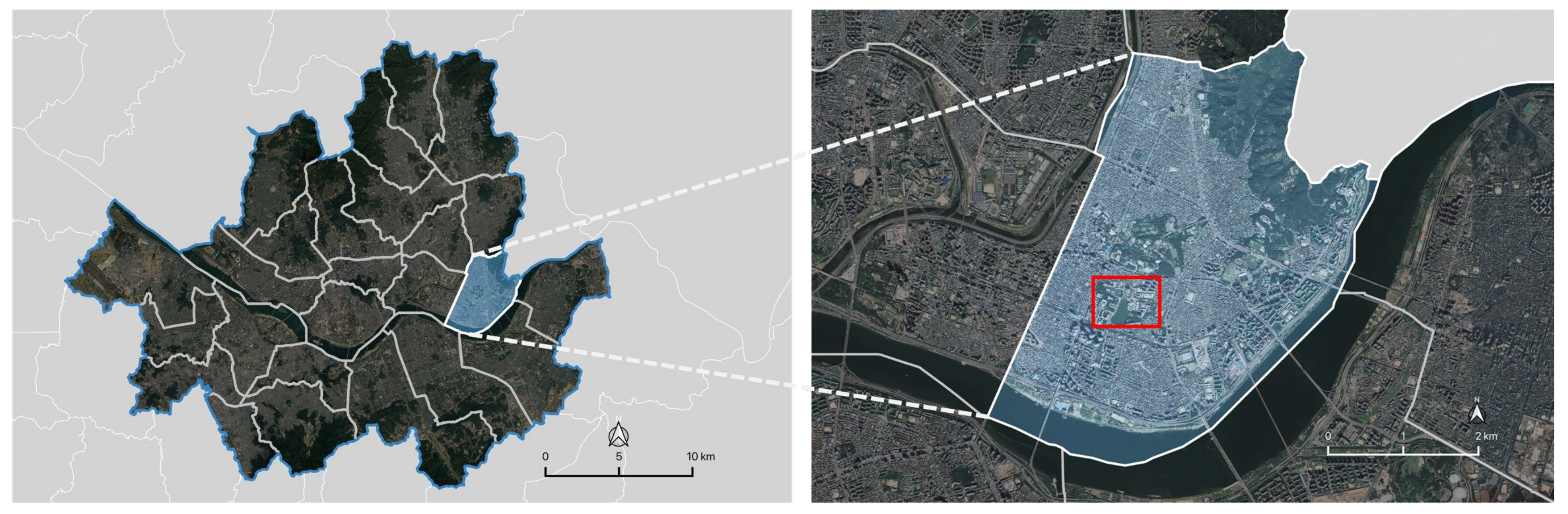
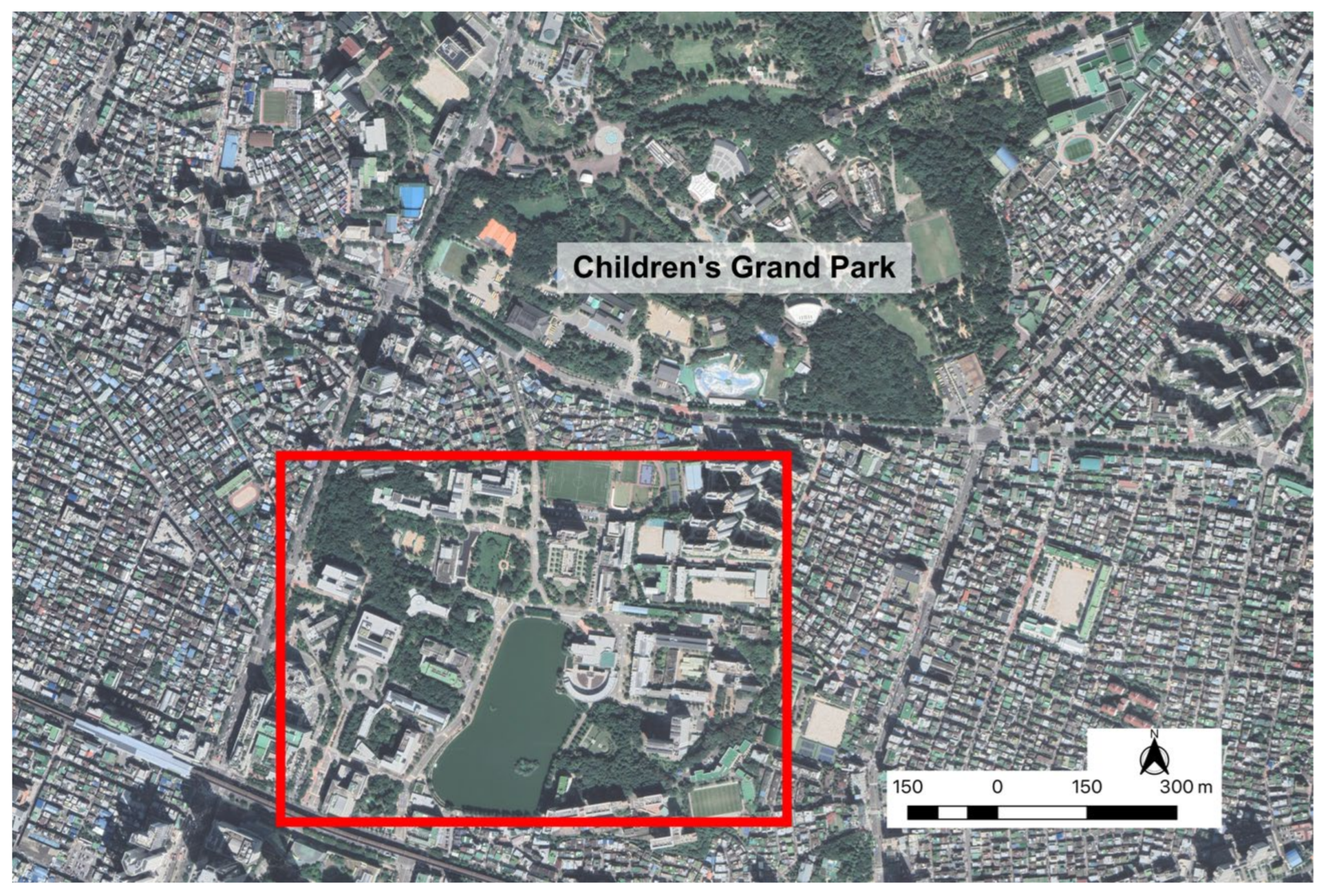
In terms of accessibility, the study utilized the main campus of Konkuk University, Seoul, South Korea, to survey the air quality at various environmental context sites (Figure 1). Customized weather stations which measured PM₁₀, PM_2.5, temperature, and humidity were installed at five locations on the campus. The university is located in the central-eastern part of Seoul, which is one of the most highly urbanized cities in the world. It is surrounded by major roads, large residential areas, and commercial skyscrapers. In particular, Children’s Grand Park, a large open space, is situated to the north. However, various types of open spaces such as lakes, forests, and playgrounds are scattered across the campus, providing different types of environmental contexts. The total area was 473,565 m², and the total number of buildings used in the modeling was 48. Furthermore, the tallest building was 61.4 m, whereas the smallest structure was 2.2 m, and the common material of the buildings was mostly reinforced concrete (Figure 2).

2.1. Air Quality Stations (Installation of PM Measuring Devices)

The PM measuring device was designed and produced in conjunction with a private company called ‘Aircock (Seoul, South Korea)’, who specialize in weather station manufacturing. Only air quality measuring devices approved by the Korean Ministry of Environment are allowed to be used in public areas, and this device was also certified by the Korea Testing & Research Institute (KTR) and Korea Conformity Laboratories (KCL). The device was named ‘Smart Aircock outdoor type 1’, and it was designed to measure a flow rate of 0.1 L per minute for the collection of PM₁₀, PM_2.5, temperature, and humidity. The method used by this device was light scattering; when 0.1 L of air flow per minute enters the sensor through the inlet, the PM and laser meet and cause light scattering. Using this generated light scattering, the size and number concentration of PM particles were determined and the PM concentrations were calculated [29]. The data measured using this process was then transmitted to the mobile device, and converted into a comma-separated value (CSV) file.

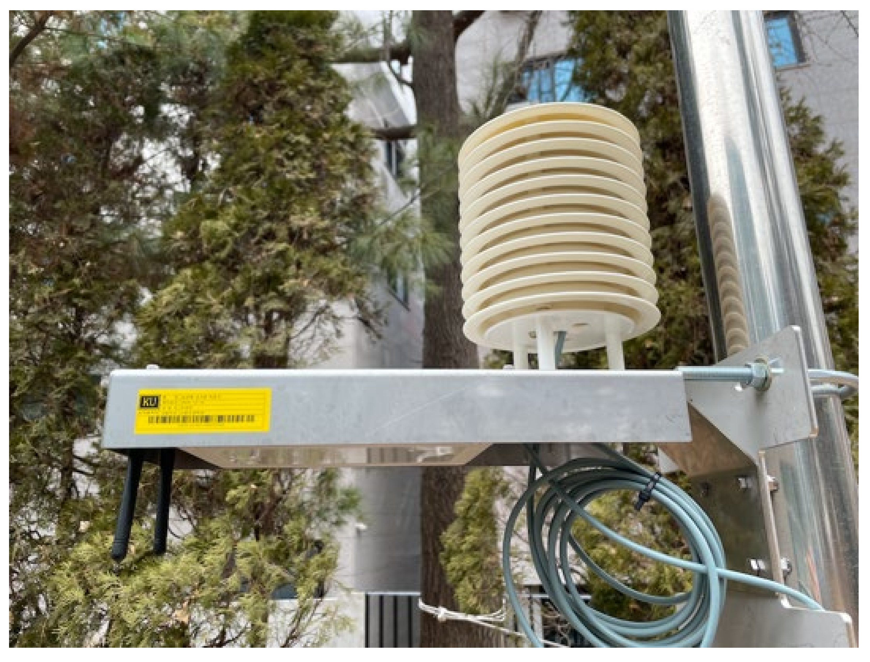
As Figure 3 indicates, it has dimensions of 40 cm × 30 cm × 15 cm, weighs 2.5 kg, and has electrical inputs of 100–240 VAC 50/60 Hz 0.5 A Max. The device was installed either mounted on the outside of a wall or fixed to a post at human height level to measure the most relevant readings for daily urban life. Four of the five devices were fixed on stainless steel posts, and one device was mounted on a concrete wall structure.

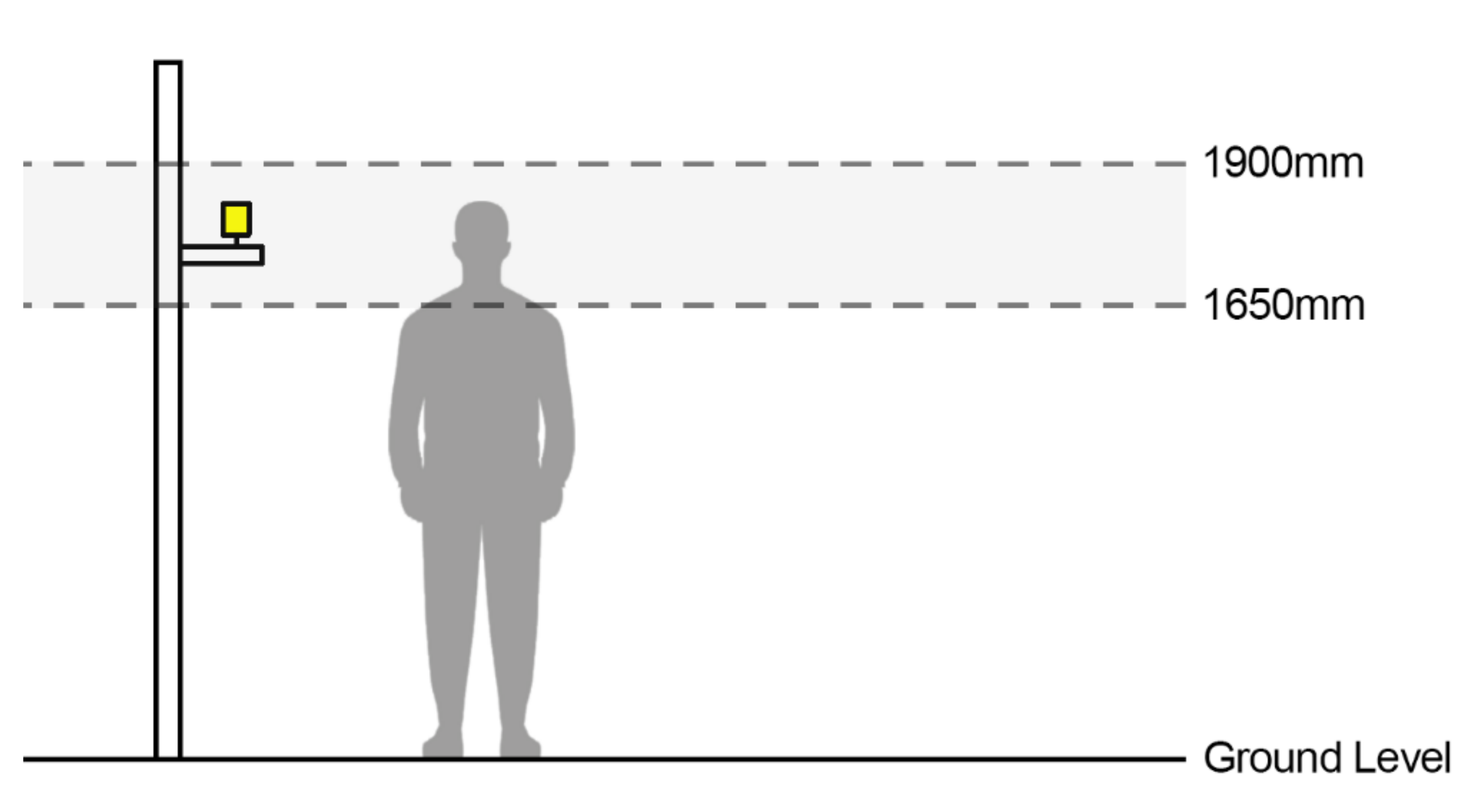
Normally, automated weather stations (AWS) are placed on higher ground, such as building roofs, to obtain steady readings and accessibility. However, such locations do not reflect the daily lives of the general public in urban areas. Therefore, unlike common AWS in other studies, this research attempts to collect credible and realistic data for ordinary urban life; the sensors were placed between 1650 mm and 1900 mm, which is the breathing height range for most people fall (Figure 4).

2.2. Environmentally Variable Contextual Settings

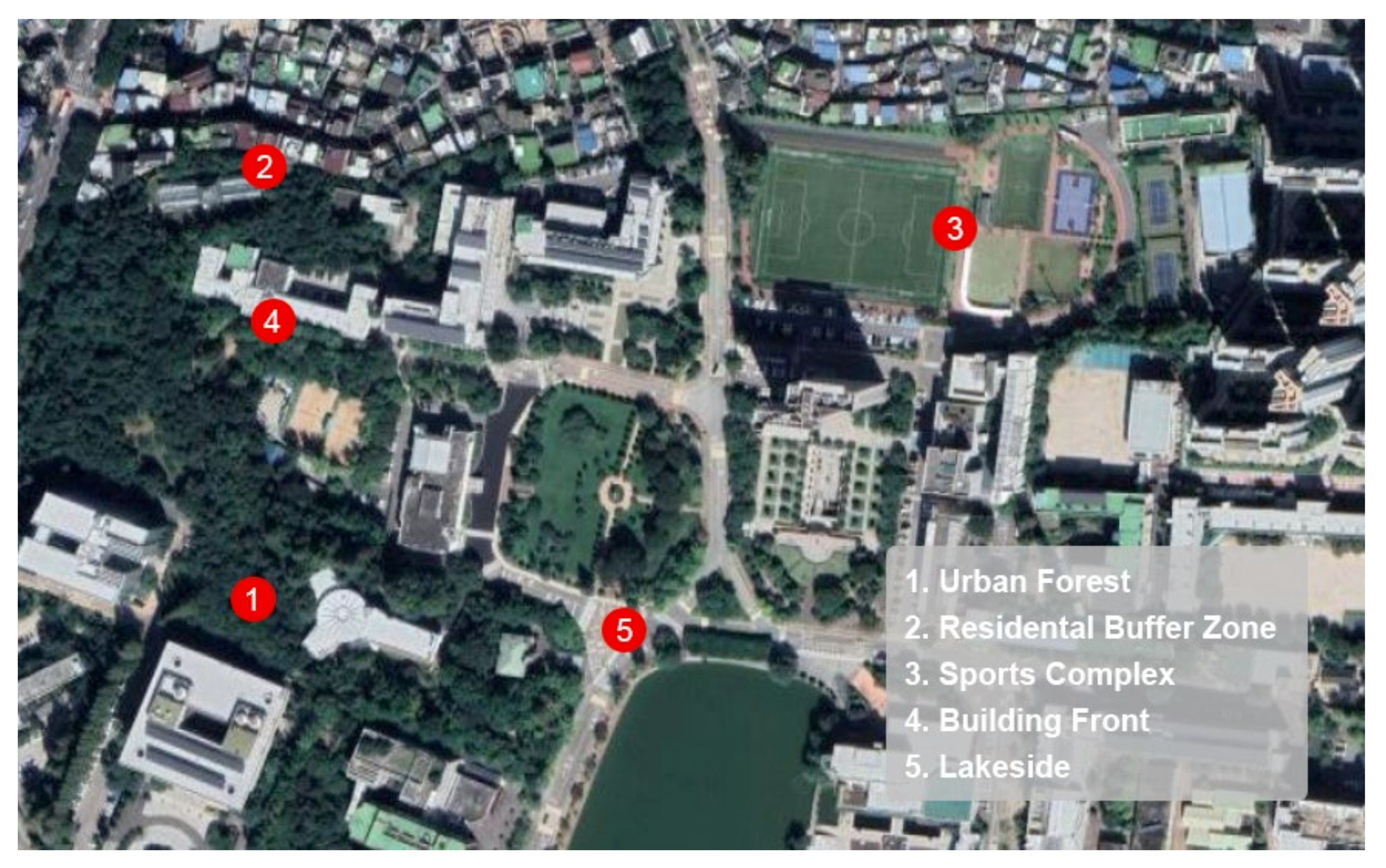
As previously described, the case study site was a university campus in Seoul. Within the campus, five locations were selected based not only on environmental contexts, but also on their openness and concealment (Figure 5).

These locations were chosen for their various spatial context settings. The five locations included forest areas heavily surrounded by woodlands, residential boundaries as buffer spaces within residential blocks, sports complexes as open and leisure spaces, building fronts, and lakesides as open and exposed contexts (

Table 1. Characteristics of PM measuring locations.

No.	Location	Spatial Context	Image
1	Urban Forest	21,090 m2 Heavy woodlands, Conifers and pine trees, enclosed space, minimum number of amenities, low use rate
2	Residential Buffer Zone	Semi-enclosed space, artificial structures, concrete, stucco blocks, little vegetation, low use rate
3	Sports Complex	25,700 m2 of open and recreational area, hard paved (concrete, tarmac), mesh fences, small structures, high use rate
4	Building Front	Semi-enclosed setting, building structures, trees, some amenities, paved with concrete blocks, high use rate
5	Lakeside	Main landmark, exposed open space with water feature (51,280 m2), surrounded by trees and shrubs, high use rate

).

First, the urban forest area is surrounded by heavy woodlands, mostly pine trees. Approximately 70 percent of the forest consists of conifers and around 30 percent of the trees are deciduous. The total area is approximately 21,090 m², and there are a minimum number of amenities, such as footpaths, benches, and exercise machines. The footpaths are hard, paved with concrete blocks, and generally this location is not heavily used by university students.

Second, the residential buffer zone is situated between the university campus grounds and the residential blocks which are generally spread around the campus. The campus boundaries are fenced with metal railings about 1.5 m heigh and of which are visually transparent. There is little vegetation, including shrubs and conifers. Artificial structures, such as concrete and stucco blocks, are dominant in this area. This is not an amenity area, and it is not used by not many people on campus.

Third, the sports complex is an open and recreational area that contains one artificial turf football pitch, two basketball courts, two tennis grounds, and a multi-use games area. Each sports ground is fenced with powder-coated mesh fences which are visually transparent. The area is approximately 25,700 m² and generally paved with hard materials such as concrete and tarmac. Small structures such as toilets, sports stands, and changing facilities exist. However, the area is mainly exposed and heavily used for recreation and sports activities.

Fourth, the building front is a typical landscaped area with semi-enclosed settings. Used as a porch area, it comprises a mixture of artificial building structures, including trees and shrubs, and some amenities such as benches and bending machines. The location is used extensively by students and staff going in and out of the buildings and the location is well linked to other buildings and open space. Additional street furniture and landscape facilities including footpaths, benches, and pergolas. It is a well-paved area with concrete blocks.

Finally, the lake is situated in the heart of the campus. Many people walk along the lake. As a main landmark, usage is very high and the lake itself is approximately 51,280 m². It is a highly exposed and open area; however, unlike location 3, which is a sports complex, it contains not only large water features, but is also surrounded by trees and shrubs. The footpaths are paved with concrete blocks and the main tree species are Himalaya Ciders and Cherries planted in order to enhance visual attractions.

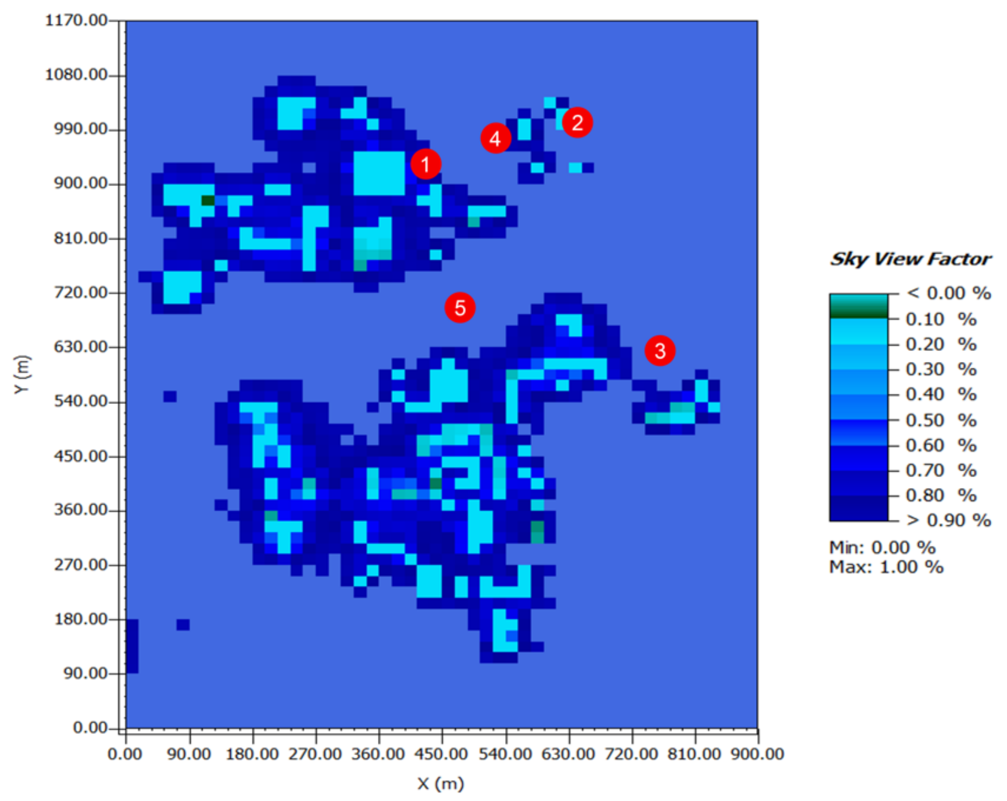
It is not always easy to categorize environmental contexts because they may contain enormous complexities. This research attempts to examine five environmentally different areas to collect PM data and to identify differences in land-use properties. Although the locations are differentiated with respect to qualitative values such as openness/enclosed, surface material, built-up structures, and vegetation, this research uses a quantitative value to categorize the characteristics of the individual locations. Sky view factors (SVFs), theoretically measured based on the three-dimensional(3D) modeling program ENVI-met, were added to measure the visibility of the sky as quantitative differences in the next section.

3. Data and Methodology

This study employed a case study method to collect real-time PM concentration levels from five environmentally different context locations. To simulate different urban settings, a university campus in Seoul was chosen, and within the campus, five qualitatively varied locations were pinned (Table 1). The qualitative values used for the sites included openness/enclosed, surface materials, built-up structures, and vegetation conditions. The measuring instrument “Smart Aircock outdoor type 1” measured a flow rate of 0.1 L per minute, stored the data every minute, and transmitted it to a mobile device to convert it into a CSV file. Additionally, we added quantitative measures as verification factors for the qualitative, real-time data. Three-dimensional modeling was conducted using ENVI-met software and, as a result, the SVF was introduced to analyze the environmental properties of each location.

3.1. Sky View Factors and ENVI-Met 3D Modeling

The sky view factor (SVF) has been commonly implemented as a critical parameter in climate research and in planning practices in urban areas [30]. The SVF is the ratio of the visible sky area of a point in space to the total sky area. It provides the relationship between the visible sky area and the covered surroundings, such as street trees or buildings. The spatial value of urban canopies varies with the x-, y-, and z-measures of the structures that define them. Therefore, the concept of SVF emerged in the 1980s to allow urban and road climatologists to develop relationships between energy and heat exchanges [31,32,33]. SVFs can be defined as a measure of the degree to which the sky is obscured by the surroundings at any given point [31].

This study employed ENVI-met software, which is a three-dimensional microclimate tool containing soil, vegetation, and heat exchange modeling capabilities [34]. The software allows users to create climatic conditions for modeling elements such as major vegetation, soil, and buildings [35]. In another study, ENVI-met was utilized to analyze the impact of roads, buildings, green areas, and other open spaces on climate conditions such as temperature and humidity [36].

To measure the concealment and openness of each location, SVFs were calculated. For the SVFs’ configuration, ENVI-met modeling was conducted for the building height and land-use properties of the campus area. Original modeling was initiated with Rhino 6 and Grasshopper packages using a series of grid cells measuring 18 m × 18 m × 3 m and the entire size of the model was 50 m × 65 m × 300 m. Surface textures were added afterwards, for instance, concrete for the buildings, water for the lake, asphalt for the roads, concrete for the car parks, and other open spaces. However, texturing is not critical for measuring SVFs.

Once the modeling of the sites was completed, SVFs from ENVI-met could be extracted to take the geographical context into account.

According to the SVF values modeled using ENVI-met (Figure 6), each location has a quantitative sky visibility value, which could be an indication of the concealment and openness of the individual locations.

3.2. Time-Series Longitudinal Analysis of PM Concentration Levels

Together with the quantitative values from the SVFs, the qualitative environmental contexts were taken into account to reflect the properties and characteristics of the five locations (Table 1 and

Table 2. Sky view factor values from ENVI-met 3D models.

Location	Names	SVFs (%)	Note
1	Urban Forest	0.50–0.60	Vegetation was not entirely modeled.
2	Residential Buffer Zone	0.10–0.20
3	Sports Complex	-	Is not calculated. *
4	Building Front	0.80–0.90
5	Lakeside	-	Is not calculated. *

* SVF values in open spaces with no built-in structures were not calculated.

). Then, the statistical software RStudio (version 3.3.0+) was used to perform a longitudinal analysis of PM concentration levels in comparison to the geographically weighted five locations. Within Rstudio, visualization works were performed using ggplot2 (version 3.4.0) packages.

The real-time data collected was too large to handle a period of more than one year; therefore, a resampling process was conducted using the Pandas software library in Python (version 3.11).

4. Results and Discussion

This research employed a case study of a university campus in an urban area. Five environmentally different locations within the campus were chosen to install PM-measuring devices and collect real-time PM concentration levels recorded at one-minute intervals between November 2021 and January 2023. In terms of the data availability, only the datasets from November 2021 to November 2022 were usable for all five locations.

In order to identify the severity of the measured PM concentrations, a comparison between the WHO’s air quality standards and the measured data was performed first.

The World Health Organization (WHO) provides air quality guidelines (AQG) to help governments improve citizens’ health by reducing air pollution [37].

Table 3. Comparison of measured PM concentration values and WHO 2021 air quality guidelines (AQG, highlighted in gray).

Location	WHO 2021 AQGs (Annual Average, mg/m3)		Annual Average (mg/m3) *		WHO 2021 AQGs (24-Hour Average, mg/m3)		MAX (24-Hour Average, mg/m3) **		MIN (24-Hour Average, mg/m3) ***
	PM10	PM2.5	PM10	PM2.5	PM10	PM2.5	PM10	PM2.5	PM10	PM2.5
Urban Forest	15	5	18	13	45	15	68	50	4	3
Residential Buffer			21	16			121	96	3	2
Sports Complex			32	24			178	136	3	2
Building Front			33	23			124	103	1	0.3
Lakeside			41	34			85	72	1	0.4

* Annual average PM value during study period (13 months). ** Average daily (24 h) maximum PM value during study period. ***Average daily (24 h) minimum PM value during study period.

indicates the comparison of this research’s annual mean, maximum, and minimum PM (PM₁₀ and PM_2.5) concentration values against the annual and 24-hour averaging PM concentrations from the recommended 2021 AQG levels. Comparing the annual average values, the measured values at all the locations were higher than the WHO’s AQG levels. In particular, the PM values at the lakeside location exceeded the WHO’s AQG levels the most; the values at the urban forest location also exceeded the WHO’s AQG levels, but they were the closest to the WHO’s AQG levels.

For the 24-hour average values, the daily average maximum values during the study period at all locations exceeded the WHO’s AQG levels. Even in the urban forest location, which showed the lowest values, the PM_2.5 concentration was well above the WHO’s AQG levels. However, the daily average minimum values were lower than the WHO’s AQG levels at all locations and were the lowest at the building front location. Except for the minimum values, the urban forest location had the lowest values both for the annual average and the maximum values.

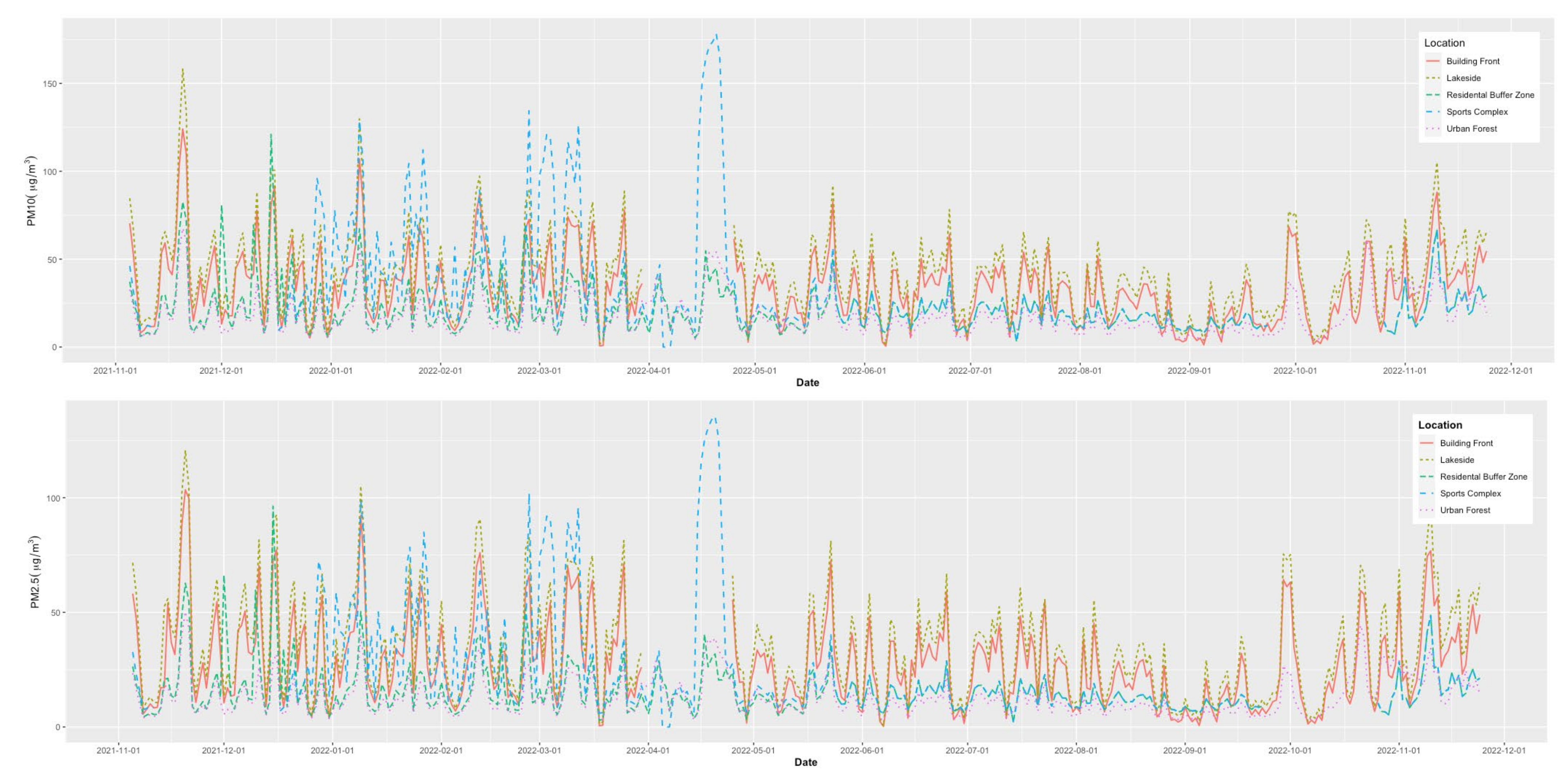
With the measured data, the researchers initially started to visualize the every minute measurement of PM₁₀ and PM_2.5 in a time-series format for the collected datasets between November 2021 and November 2022. However, this could not be illustrated effectively because of the density of the data. Therefore, this research used resampling tools in order to obtain the daily average values from the minutely collected data and to illustrate the five locations, as shown in Figure 7.

According to Figure 7, the differences between PM₁₀ and PM_2.5 were minimal. There were also exceptional pattern values such as the PM levels in April at the sports complex location; however, this could have been a localized event caused by the intensive sports and leisure activities on the university campus during the spring. Moreover, the PM measuring sensors were sensitive because they were installed at human breathing heights, which were in the range of 1650 mm to 1900 mm from the ground level in the study (Figure 4).

For the scale of the time-series analysis shown in Figure 7, it is not easy to comparatively analyze the numerical values of the individual locations; however, an overall trend can be drawn. For example, throughout the year between November 2021 and November 2022, regardless of seasonal changes, the urban forest location was low in PM concentration levels. Comparing the lakeside and building front locations, higher levels of PM₁₀ and PM_2.5 were consistently observed at the lakeside location.

To investigate the geographical differences among the five locations in detail, a resampling of PM₁₀ and PM_2.5 was repeated from daily to monthly average values, as illustrated in Figure 8.

Unlike Figure 7, which was based on hourly datasets, Figure 8 illustrates a clear comparable value of the PM concentration levels at each location. First, there is not much difference between the PM₁₀ and PM_2.5 levels, which is similar to the results shown in Figure 7. However, each location showed a clear hierarchical pattern in the concentration levels, except for the sports complex, whose changes varied. The PM levels at the lakeside were constantly high, followed by the building front. The residential buffer zones and urban forests showed similar patterns of lower PM concentrations, but the urban forests were marginally lower than the residential buffer zones. With the exception of the sports complex location, these results illustrate that openness/enclosure is the main factor affecting PM concentration levels. According to Figure 8, the concentration level of PM was high in the spring and low in the autumn at the sports complex location. Therefore, it can be concluded that more exposed locations have denser levels of PM concentration, which include the lakeside, building front, residential buffer zone, and urban forest in that order, excepting the sports complex location. Physical structures or any obstacles could block PM penetration; in particular, vegetation and pine tree forests, in this case, seemed to be effective in filtering PM infiltrations. These results also corresponded to the SVF values for each location.

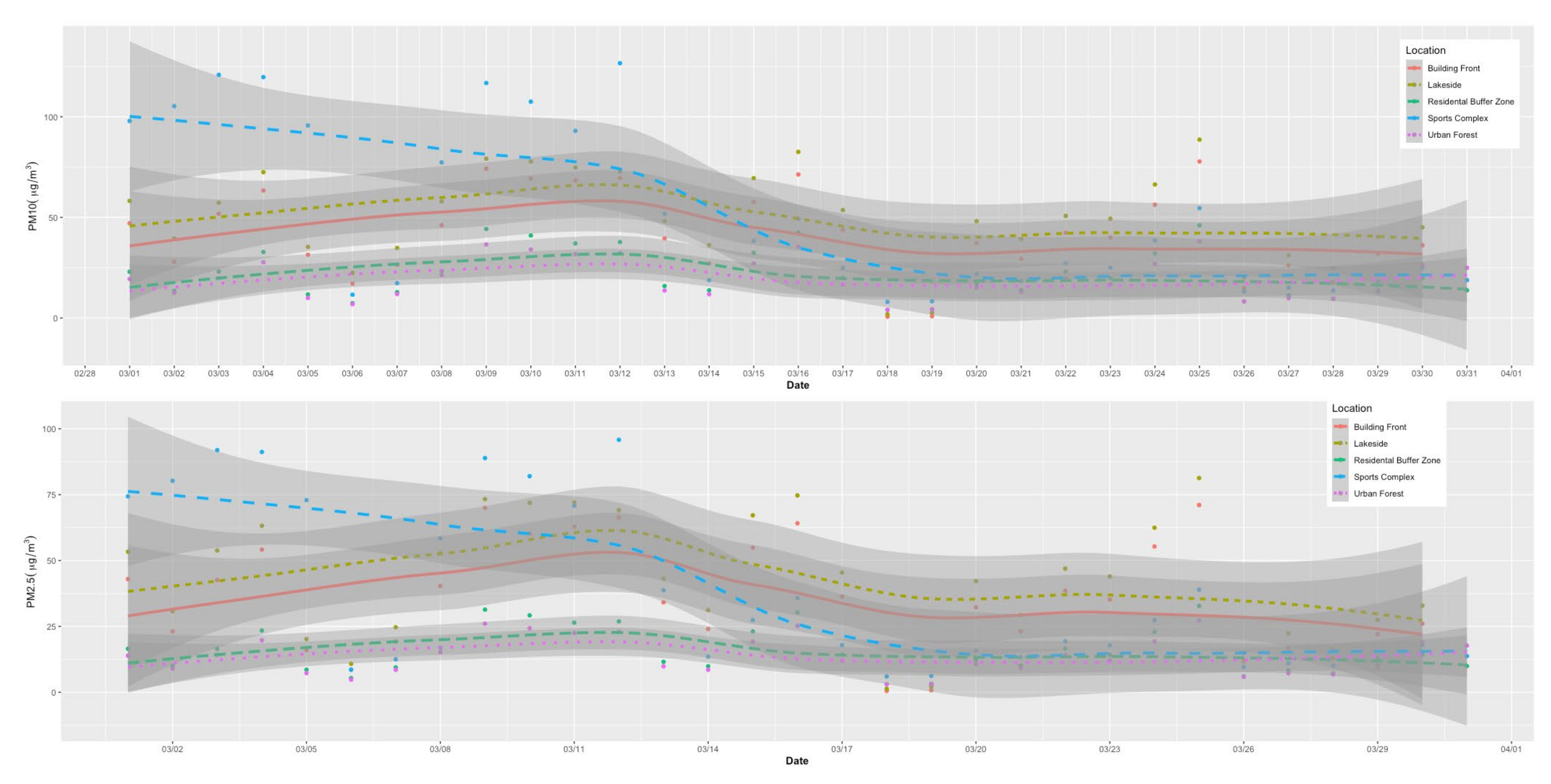
Additionally, this research investigated the PM levels for each location in March 2022, when the overall PM concentrations were the highest within the year. This is illustrated in Figure 9, which was created using the daily average values of PM₁₀ and PM_2.5 by resampling from the original measured data from the individual real-time sensors.

In Figure 9, the daily average values from the collected data are presented in a scatterplot for the duration of March 2022. Then, LOESS (weighted scatterplot smoothing) was implemented to provide an overall impression of the trends without fitting parametric models to allow for flexibility in understanding the overall tendencies. By doing so, this analysis effectively explored the trends in PM level changes in the specific environmental contexts.

In this analysis (Figure 9), the spatial hierarchy based on the environmental context was demonstrated more clearly than the results in Figure 7 and Figure 8, which were yearly time-series analyses. However, it needs to be mentioned that the PM₁₀ and PM_2.5 concentration levels at the sports complex location behaved unpredictably, showing patterns similar to those in Figure 7 and Figure 8. Therefore, apart from the sports complex location, the PM concentration levels at the four locations illustrated certain patterns and hierarchies. First, there could be two main groups: those with higher and lower PM levels. The higher group is composed of the lakeside and building-front locations. The measured PM levels in the higher group were recorded to be approximately 10 to 30 mg/m³ higher than in the lower group, which includes the residential buffer zones and the urban forest locations. Then, the PM level gap between the lakeside and building front locations within the higher group was continuously steady at approximately 10 mg/m³. The measured PM levels in the lower group, the residential buffer zone and the urban forest locations, were relatively similar. The differences between the residential buffer zone and the urban forest were quite narrow, ranging from 0 to 6 mg/m³.

In summary, the urban forest location showed the lowest level of PM concentrations, and the residential buffer zone location had the next highest PM levels by a narrow margin. The third highest PM levels were observed at the building front location, with an average gap of 20 mg/m³. Finally, the highest PM level was at the lakeside location, which was approximately 10 mg/m³ higher in general.

This research has sought to explain why PM concentration levels vary exceptionally at the sports complex location. This research concluded that due to extensive sports and leisure events, there were temporal rises and falls in the PM concentration levels that affected overall air quality. In particular, because the PM sensor was installed at the human breathing level, the sensitivity was increased.

According to Figure 7, Figure 8, and Figure 9, the more enclosed a location is, the lower the PM₁₀ and PM_2.5 concentrations are. In particular, the location enclosed by the forest, where the majority of the species were conifers and pine trees, was demonstrated to have better air quality, based on PM₁₀ and PM_2.5 levels, as compared to built-up structures such as reinforced concrete buildings.

In addition, SVFs were implemented to express the variances among the environmental contexts quantitatively. The SVF readings strongly corresponded with the overall research results; however, the SVF values were not all fit at some locations because the SVFs were calculated mainly using artificially built-up structures. The exclusion of localized vegetation and detailed elements caused some discrepancies between the SVF values and the actual environmental contexts. These discrepancies mean that the SVF values do not reflect what is really happening in those locations.

5. Conclusions

Since the beginning of industrialization and urbanization, the world has suffered from large numbers of air pollutants in urban areas. Recent threats from PM₁₀ and PM_2.5 have emerged because of their size and potential to create serious health problems, including asthma, heart-related diseases, and respiratory diseases. Despite the recognized importance of research using the GWR or LUR models for PM concentration levels in urban areas, there is little research that uses actual measured data, such as real-time data collection.

Therefore, the purpose of this study was to explore variations in air quality, particularly PM densities, in different land-use types within urban areas. A case study method was employed to determine the aims and purposes of the study. Real-time sensors that checked the PM₁₀ and PM_2.5 concentration levels at a height of approximately 1700 mm were installed at five locations with different environmental characteristics. Recorded PM₁₀ and PM_2.5 levels in human breath were collected for the five locations in the period between November 2021 and January 2023. The five locations were an urban forest, residential buffer zone, sports complex, building front, and lakeside. The research tried to emulate common spaces in urban areas, differentiating between openness/enclosure, amount of green infrastructure, and land usage.

Three time-series analysis steps were performed. First, the collected data of the PM₁₀ and PM_2.5 concentration levels recorded every minute were resampled into daily average values and then visualized for the five locations in the period between November 2021 and November 2022. Second, the collected PM₁₀ and PM_2.5 concentration levels were resampled into monthly average values and then visualized to better understand the pattern of changes at each location. Finally, data from March 2022, which was the worst month, were visualized to provide a detailed analysis.

Based on the analysis of a three-phase time-series and SVF calculation, the more a space is enclosed, the lower the level of PM₁₀ and PM_2.5 concentration detected overall. In particular, the space surrounded by a conifer forest showed better air quality than spaces enclosed by reinforced concrete buildings. Some discrepancies seen at the sports complex could be explained by the overly sensitive PM sensors which were installed at human breathing levels, as well as the intensive sports and leisure activities conducted there. Therefore, the research concluded that physical structures and obstacles could affect the concentration levels of PM₁₀ and PM_2.5. In particular, when the physical structures comprised a group of trees or forests, this had a positive effect on reducing the concentration levels of PM₁₀ and PM_2.5.

In addition to these findings, similar follow-up studies that will take into account more diverse environmental contexts, such as the denser urban fabric, including high-traffic roads and high-rise buildings, are expected to contribute to policy and decision-making processes in landscape architecture and urban design. Moreover, these studies could serve as spatial guidelines for public health and welfare within urban life. The methodology implemented in this study attempted to consider a both qualitative and quantitative analysis of the classification of environmental variances, in which surrounding contexts and SVFs were employed. However, analyzing the environment in a quantitative way is ambiguous. Consequently, SVFs were not as effective as the study initially anticipated. Hence, new methods to provide accurate quantitative classifications of the environment need to be conducted in future studies; for example, if a specific measurement is used such as SVFs, the SVFs also need to contain vegetation rather than only artificial structures such as building blocks.