
Urban Structure Changes in Three Areas of Detroit, Michigan (2014–2018) Utilizing Geographic Object-Based Classification
Abstract
:1. Introduction
1.1. Urban Shrinking Phenomenon
1.2. Geographic Object-Based Image Analysis
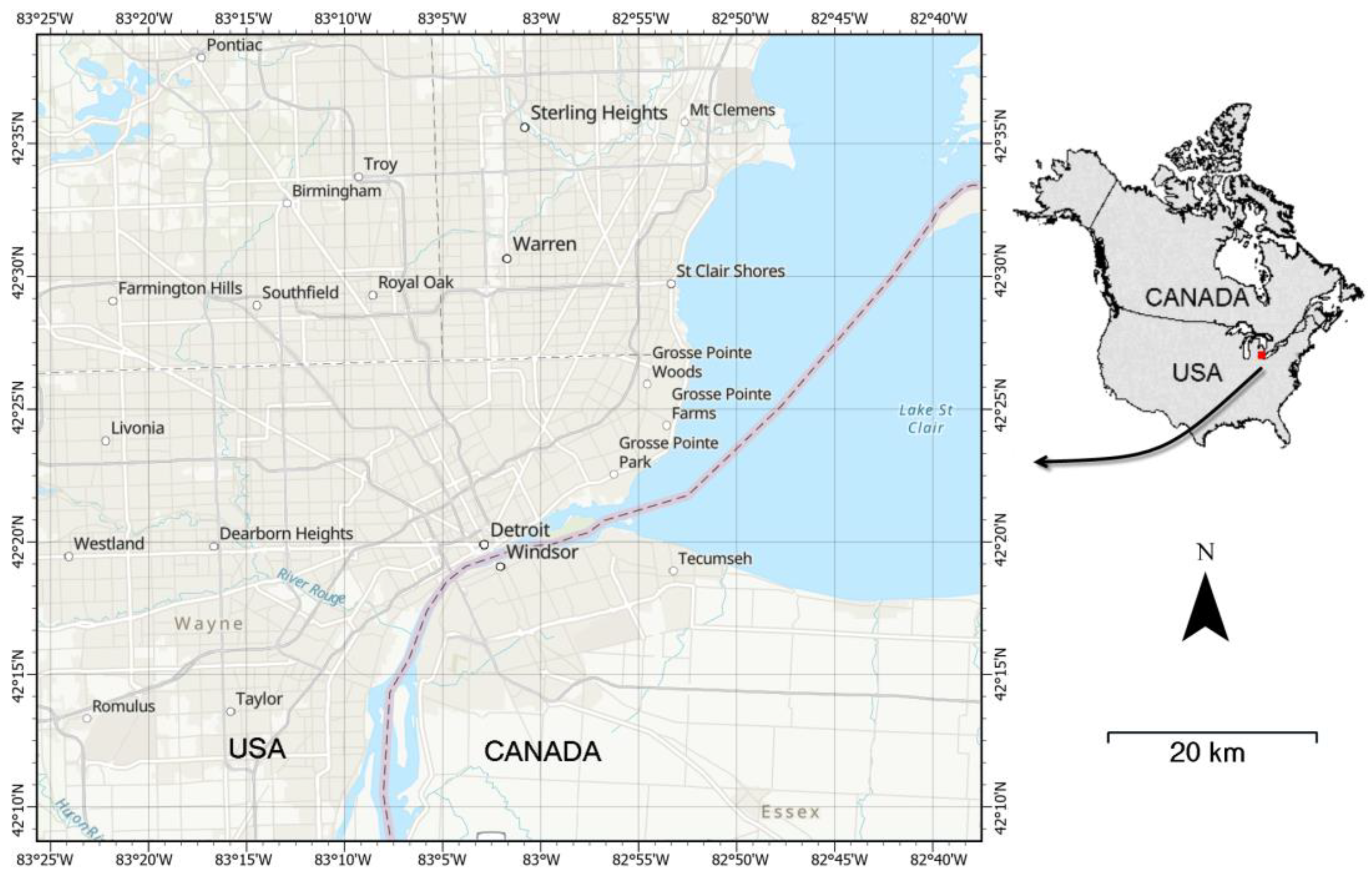
2. Study Area and Previous Urban Analysis
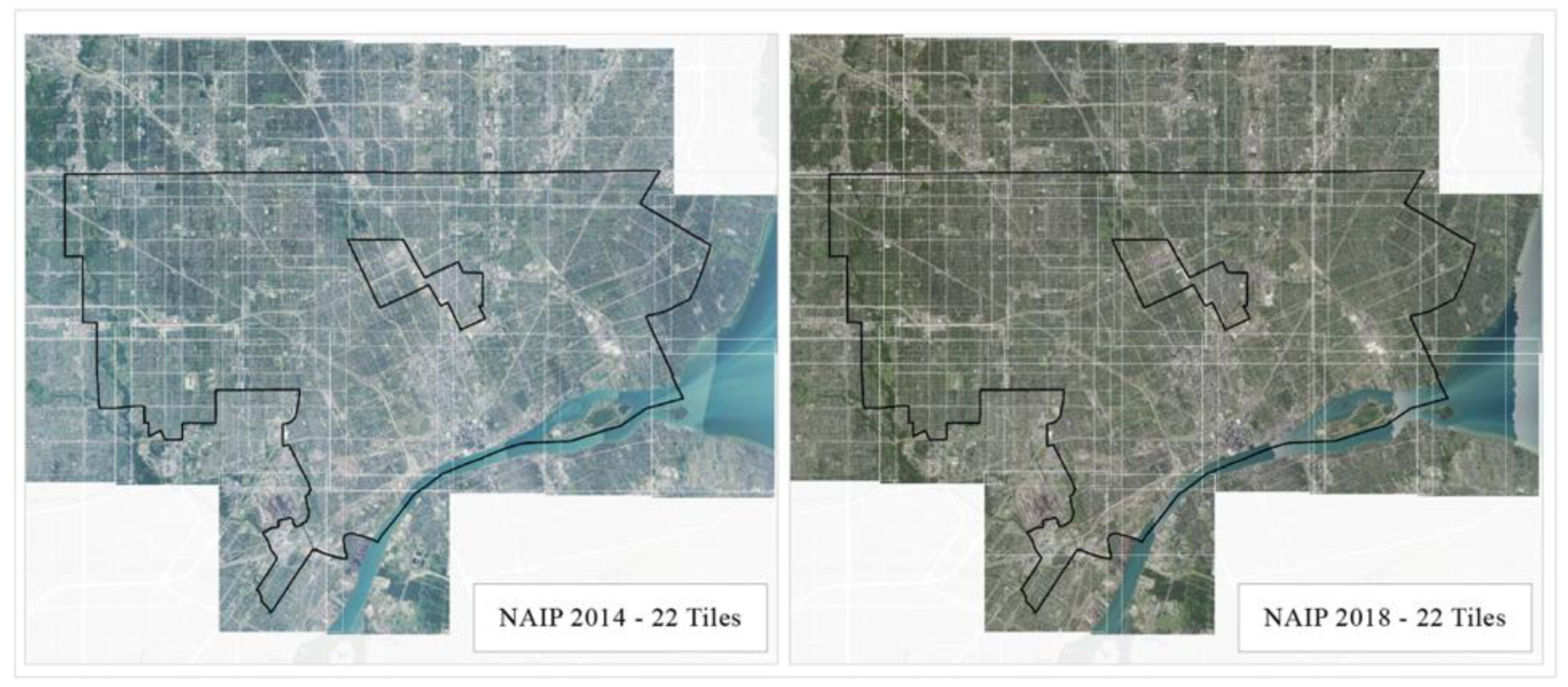
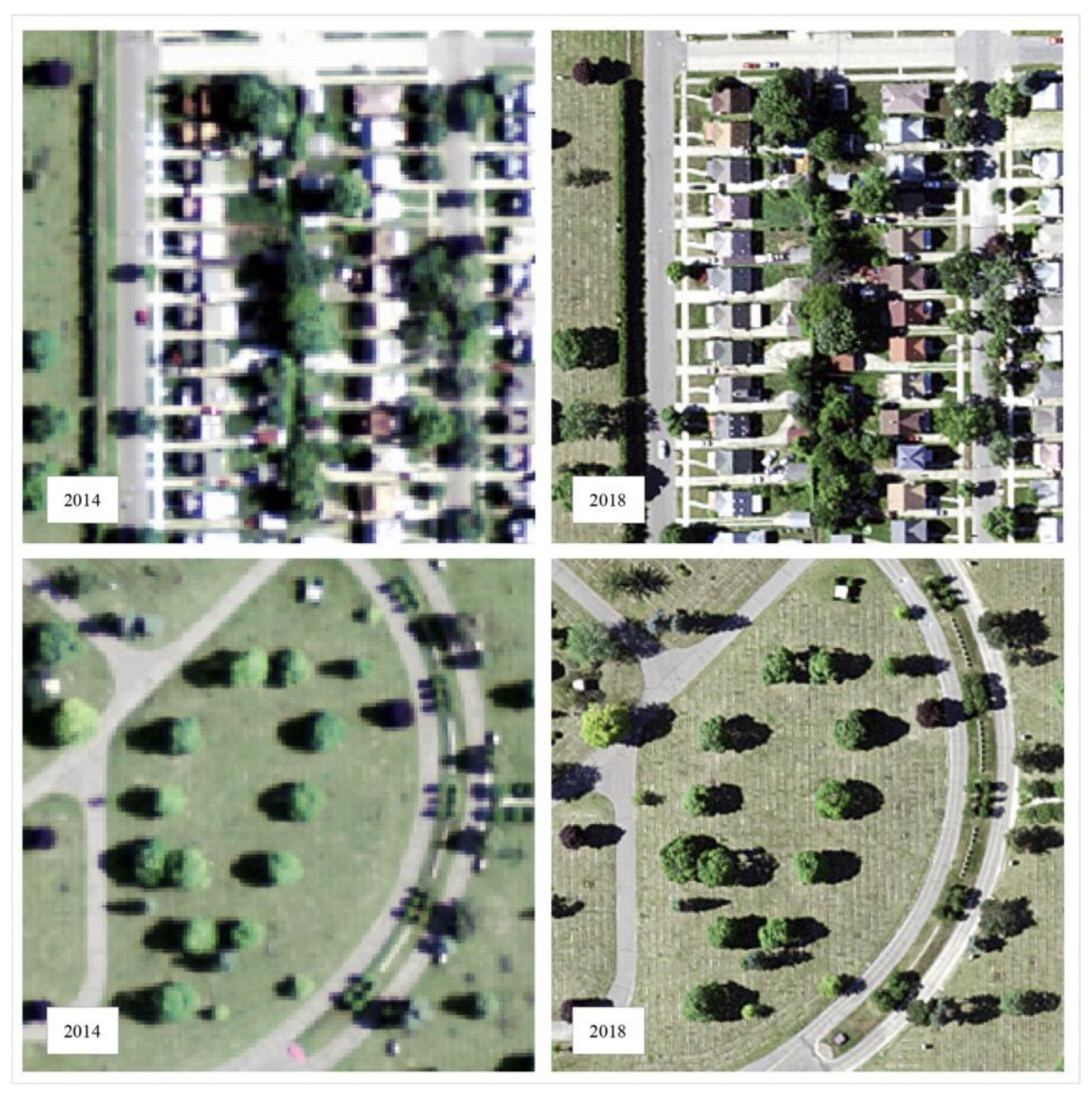
2.1. Airborne Imagery
2.2. Study Area Data and NAIP Imagery
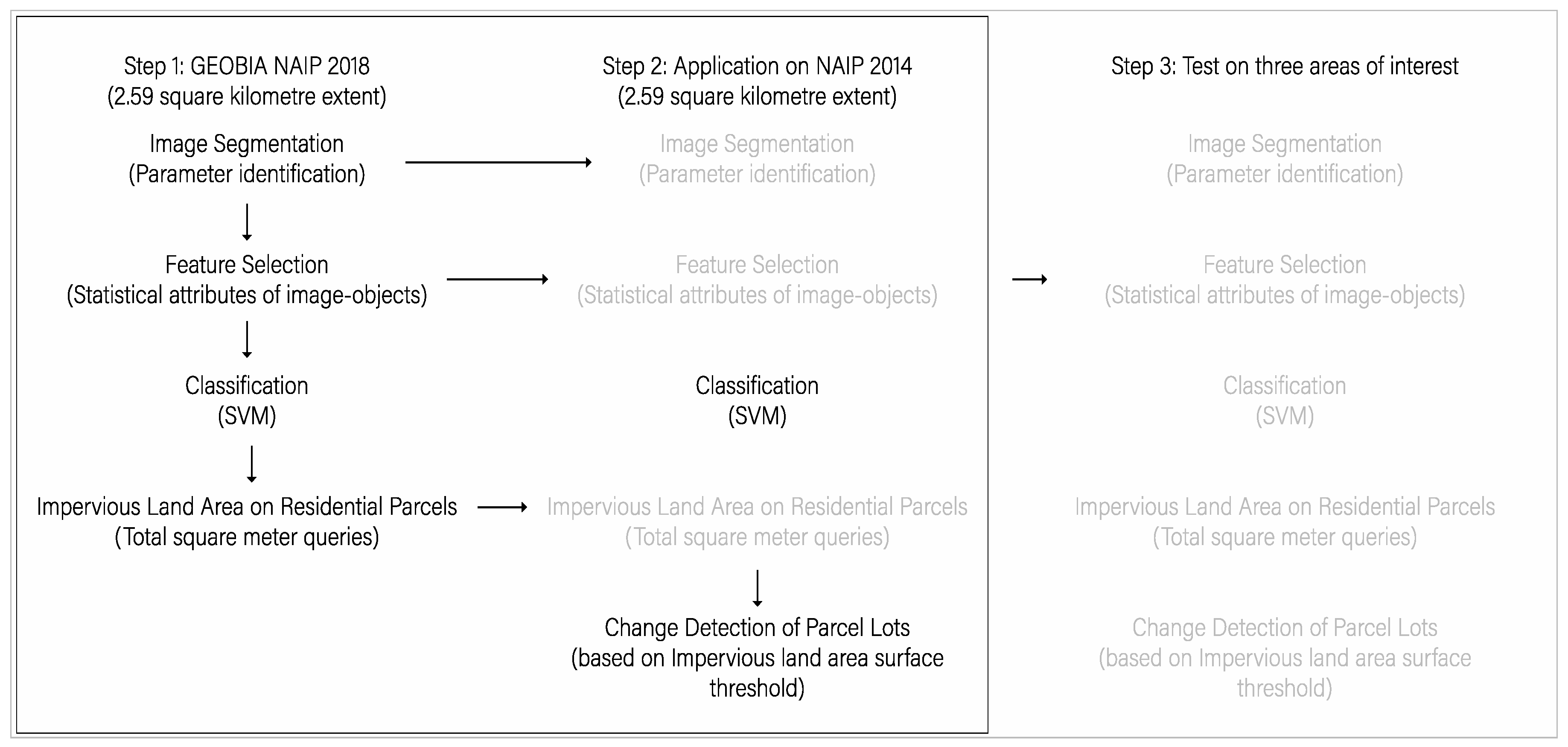
2.3. Image Processing and Classification Workflow
2.4. Image Segmentation
3. GEOBIA Methods
4. Results and Analysis
4.1. Image Segmentation, Feature Selection and Classification Accuracy
4.2. Research Challenges
5. Conclusions
Author Contributions
Funding
Data Availability Statement
Conflicts of Interest
References
- Forsythe, K.W.; Waters, N.M. The Utilization of Image Texture Measures in Urban Change Detection. Photogramm. Fernerkund. Geoinf. 2006, PFG 4, 287–296. [Google Scholar]
- Sidhu, N.; Rishi, M.S.; Singh, R. Spatio-Temporal Study of the Distribution of Land Use and Land Cover Change Pattern in Chandigarh, India Using Remote Sensing and GIS Techniques. In Geostatistical and Geospatial Approaches for the Characterization of Natural Resources in the Environment; Raju, J.N., Ed.; Springer: New York, NY, USA, 2016; pp. 785–789. [Google Scholar]
- Shrestha, S.; Cui, S.; Xu, L.; Wang, L.; Manandhar, B. Impact of Land Use Change Due to Urbanisation on Surface Runoff Using GIS-based SCS-CN Method: A case study of Xiamen City, China. Land 2021, 10, 839. [Google Scholar] [CrossRef]
- Hossain, M.D.; Chen, D. Segmentation for Object-Based Image Analysis (OBIA): A Review of Algorithms and Challenges from Remote Sensing Perspective. ISPRS J. Photogramm. Remote Sens. 2019, 150, 115–134. [Google Scholar] [CrossRef]
- United Nations, Department of Economic and Social Affairs. World Urbanization Prospects: The 2018 Revision; United Nations: New York, NY, USA, 2019. [Google Scholar]
- Hartt, M. The Diversity of North American Shrinking Cities. Urban Stud. 2018, 13, 2946–2959. [Google Scholar] [CrossRef]
- Thompson, E.S.; de Beurs, K.M. Tracking the Removal of Buildings in Rust Belt Cities with Open-Source Geospatial Data. Int. J. Appl. Earth Obs. Geoinf. 2018, 73, 471–481. [Google Scholar] [CrossRef]
- Burkholder, S. The new ecology of vacancy: Rethinking land use in shrinking cities. Sustainability 2012, 4, 1154–1172. [Google Scholar] [CrossRef] [Green Version]
- Deng, C.; Ma, J. Viewing urban decay from the sky: A multi-scale analysis of residential vacancy in a shrinking U.S., city. Landsc. Urban Plan. 2015, 141, 88–99. [Google Scholar] [CrossRef]
- Blaschke, T. Object Based Image Analysis for Remote Sensing. ISPRS J. Photogramm. Remote Sens. 2010, 65, 2–16. [Google Scholar] [CrossRef] [Green Version]
- Hay, G.J.; Castilla, G. Geographic Object-Based Image Analysis (GEOBIA): A New Name for a New Discipline. In Object Based Image Analysis; Blaschke, T., Lang, S., Hay, G., Eds.; Springer: New York, NY, USA, 2008; pp. 93–112. [Google Scholar]
- Ma, L.; Li, M.; Blaschke, T.; Ma, X.; Tiede, D.; Cheng, L.; Chen, Z.; Chen, D. Object0based change detection in urban areas: The effects of segmentation strategy, scale, and feature space on unsupervised methods. Remote Sens. 2016, 8, 761. [Google Scholar] [CrossRef] [Green Version]
- Mendiratta, P.; Gedam, S. Assessment of urban growth dynamics in Mumbai Metropolitan Region, India using object-based image analysis for medium-resolution data. Appl. Geogr. 2018, 98, 110–120. [Google Scholar] [CrossRef]
- Maxwell, A.E.; Strager, M.P.; Warner, T.A.; Ramezan, C.A.; Morgan, A.N.; Pauley, C.E. Large-Area, high spatial resolution land cover mapping using Random Forests, GEOBIA, and NAIP orthophotography: Findings and recommendation. Remote Sens. 2019, 11, 1409. [Google Scholar] [CrossRef] [Green Version]
- Norman, M.; Mohd Shahar, H.; Mohamad, Z.; Rahim, A.; Amri Mohd, F.; Zulhaidi Mohd Shafri, H. Urban building detection using object-based image analysis (OBIA) and machine learning (ML) algorithms. IOP Conf. Ser. Earth Environ. Sci. 2021, 620, 12010. [Google Scholar] [CrossRef]
- Toney, C.; Liknes, G.; Lister, A.; Meneguzzo, D. Assessing Alternative Measures of Tree Canopy Cover: Photo-Interpreted NAIP and Ground-Based Estimates. In Proceedings of the Monitoring Across Borders: 2010 Joint Meeting of the Forest Inventory and Analysis (FIA) Symposium and the Southern Mensurationists, Knoxville, TN, USA, 5–7 October 2010; McWilliams, W., Roesch, F.A., Eds.; U.S. Department of Agriculture, Forest Service, Southern Research Station: Asheville, NC, USA, 2012; pp. 209–215. [Google Scholar]
- Yen, C.; Stow, D.A.; Toure, S.I. A Histogram Curve-Machine Approach for Object-Based Image Analysis of Urban Land Use. GI-Forum 2020, 8, 160–174. [Google Scholar]
- Johnson, B.A.; Ma, L. Image Segmentation and Object-Based Image Analysis for Environmental Monitoring: Recent Areas of Interest, Researchers’ Views and The Future Priorities. Remote Sens. 2020, 12, 1772. [Google Scholar] [CrossRef]
- United States Census Bureau. Available online: https://www2.census.gov/geo/docs/maps-data/data/gazetteer/2021_Gazetteer/2021_gaz_place_26.txt (accessed on 15 March 2021).
- United States Census Bureau. Available online: https://www.census.gov/quickfacts/fact/dashboard/detroitcitymichigan/POP010220 (accessed on 15 March 2021).
- Xie, Y.; Gong, H.; Lan, H.; Zeng, S. Examining Shrinking City of Detroit in the Context of Socio-Spatial Inequalities. Landsc. Urban Plan. 2018, 177, 350–361. [Google Scholar] [CrossRef]
- United States Census Bureau. Available online: https://www.census.gov/library/working-papers/1998/demo/POP-twps0027.html (accessed on 15 March 2021).
- Ager, S. Taking back Detroit. Natl. Geogr. 2015, 227, 56–83. [Google Scholar]
- The Economist Newspaper. Available online: https://www.economist.com/united-states/2017/07/27/how-the-riots-of-50-years-ago-changed-detroit (accessed on 15 March 2021).
- The Economist Newspaper. Available online: https://www.economist.com/united-states/2017/09/16/in-detroit-the-end-of-blight-is-in-sight (accessed on 15 March 2021).
- Hoalst-Pullen, N.; Patterson, M.W.; Gatrell, J. Empty Spaces: Neighbourhood Change and the Greening of Detroit, 1975–2005. Geocarto Int. 2011, 26, 417–434. [Google Scholar] [CrossRef]
- Foster, A.; Newell, J.P. Detroit’s Lines of Desire: Footpaths and Vacant Land in the Motor City. Landsc. Urban Plan. 2019, 189, 260–273. [Google Scholar] [CrossRef]
- Goodman, A.C. Detroit Housing Rebound Needs Safe Streets, Good Schools. Wayne State University. 2004. Available online: https://allengoodman.wayne.edu/RESEARCH/PUBS/a09-87052.htm (accessed on 15 March 2021).
- Data Driven Detroit. Available online: https://portal.datadrivendetroit.org/datasets/D3::motor-city-mapping-enhanced-file-october-1st-survey-results/about (accessed on 15 March 2021).
- Detroit Future City. Available online: https://detroitfuturecity.com/wp-content/uploads/2015/06/DFC-Open-Space–Report-1.pdf (accessed on 15 March 2021).
- LOST Magazine. Available online: http://lostmag.matthewbrian.com/issue42/detroit.php#_ednref21 (accessed on 15 March 2021).
- City of Detroit. Available online: https://data.detroitmi.gov/datasets/detroitmi::completed-residential-demolitions/about (accessed on 15 March 2021).
- Detroit Data Collaborative. Available online: https://datadrivendetroit.org/files/DRPS/Detroit%20Residential%20Parcel%20Survey%20OVERVIEW.pdf (accessed on 15 March 2021).
- Data Driven Detroit. Available online: https://datadrivendetroit.org/files/DCPS/D3_NNIP_040414.pdf (accessed on 15 March 2021).
- Giner, N.M.; Polsky, C.; Pontius, R.G.; Runfola, D.M. Understanding the Social Determinants of Lawn Landscapes: A Fine-Resolution Spatial Statistical Analysis in Suburban Boston, Massachusetts, USA. Landsc. Urban Plan. 2013, 111, 25–33. [Google Scholar] [CrossRef]
- Merry, K.; Siry, J.; Bettinger, P.; Bowker, J.M. Urban Tree Cover in Detroit and Atlanta, USA, 1951–2010. Cities 2014, 41, 123–131. [Google Scholar] [CrossRef]
- Ellis, E.A.; Mathews, A.J. Object-Based Delineation of Urban Tree Canopy: Assessing Change in Oklahoma City, 2006–2013. Comput. Environ. Urban Syst. 2019, 73, 85–94. [Google Scholar] [CrossRef]
- United States Department of Agriculture. Available online: https://www.fsa.usda.gov/programs-and-services/aerial-photography/imagery-programs/naip-imagery/ (accessed on 15 March 2021).
- National Agriculture Imagery Program (NAIP). United States Department of Agriculture. Available online: https://www.fsa.usda.gov/Assets/USDA-FSA-Public/usdafiles/APFO/support-documents/pdfs/naip_infosheet_2017.pdf (accessed on 15 March 2021).
- Huang, S.; Tang, L.; Hupy, J.P.; Wang, Y.; Shao, G. A Commentary Review on the Use of Normalized Difference Vegetation Index (NDVI) in the Era of Popular Remote Sensing. J. For. Res. 2020, 32, 1–6. [Google Scholar] [CrossRef]
- City of Detroit. Available online: https://data.detroitmi.gov/datasets/detroitmi::parcels-2/about (accessed on 15 March 2021).
- City of Detroit. Available online: https://data.detroitmi.gov/datasets/detroitmi::current-city-of-detroit-neighborhoods/about (accessed on 15 March 2021).
- Hussain, M.; Chen, D.; Cheng, A.; Wei, H.; Stanley, D. Change Detection from Remotely Sensed Images: From Pixel-Based to Object-Based Approaches. ISPRS J. Photogramm. Remote Sens. 2013, 80, 91–106. [Google Scholar] [CrossRef]
- Jayasekare, A.S.; Wickramasuriya, R.; Namazi-Rad, M.; Perez, P.; Singh, G. Hybrid Method for Building Extraction in Vegetation-Rich Urban Areas from very High-Resolution Satellite Imagery. J. Appl. Remote Sens. 2017, 11, 036017. [Google Scholar] [CrossRef] [Green Version]
- Shahi, K.; Sharfi, H.Z.M.; Hamedianfar, A. Road Condition Assessment by OBIA and Feature Selection Techniques Using Very High-Resolution Worldview-2 Imagery. Geocarto Int. 2017, 32, 1389–1406. [Google Scholar] [CrossRef]
- Chen, G.; Hay, G.J.; Carvalho, L.M.T.; Wulder, M.A. Object-Based Change Detection. Int. J. Remote Sens. 2012, 33, 4434–4457. [Google Scholar] [CrossRef]


| Acquisition Date | Channels | Resolution | Flight Altitude | Sensor |
|---|---|---|---|---|
| 28 June 2014 | R, G, B, NIR | 1 m | 17,500 ft 28,000 ft | Leica ADS 40 |
| 6–7 July 2018 | R, G, B, NIR | 0.6 m | 16,000 ft | Leica ADS 100 |
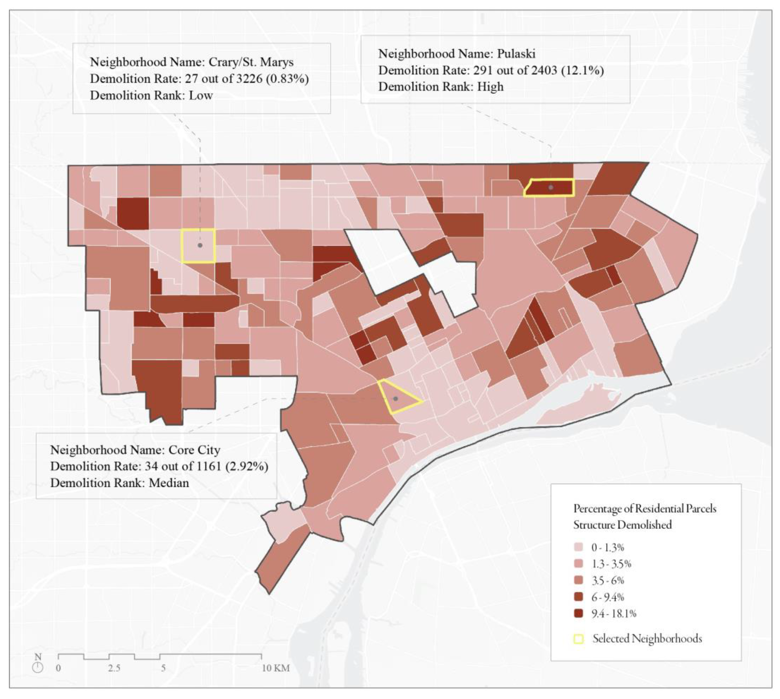
| Neighbourhood | Residential Parcel Lots | Residential Demolitions | Residential Demolition Rate |
|---|---|---|---|
| Crary/St. Mary (low) | 3226 | 27 | 0.83% |
| Core City (median) | 1161 | 34 | 2.9% |
| Pulaski (high) | 2493 | 291 | 12.1% |
| Class Name | Producer’s Accuracy | 95% Confidence Interval | User’s Accuracy | 95% Confidence Interval | Kappa Statistic |
|---|---|---|---|---|---|
| Pervious | 99.333% | (97.697% 100%) | 97.385% | (94.530% 100%) | 0.947 |
| Impervious | 97.333% | (94.421% 100%) | 99.319% | (97.650% 100%) | 0.986 |
| Overall accuracy: 98.333% | 95% Confidence interval (96.717% 99.948%) | ||||
| Overall kappa Statistic: 0.966 | Overall kappa variance: 0.666 | ||||
| Classified Data | Reference Data | ||
|---|---|---|---|
| Pervious | Impervious | Totals | |
| Pervious | 149 | 4 | 153 |
| Impervious | 1 | 146 | 147 |
| Totals | 150 | 150 | 300 |
| Class Name | Producer’s Accuracy | 95% Confidence Interval | User’s Accuracy | 95% Confidence Interval | Kappa Statistic |
|---|---|---|---|---|---|
| Pervious | 100% | (99.666% 100%) | 96.774% | (93.670% 0.935 99.878%) | 0.935 |
| Impervious | 96.666% | (93.460% 99.872%) | 100% | (99.655% 100%) | 1 |
| Overall accuracy: 98.333% | 95% Confidence interval (96.717% 99.948%) | ||||
| Overall kappa statistic: 0.966 | Overall kappa variance: 0.000 | ||||
| Classified Data | Reference Data | ||
|---|---|---|---|
| Pervious | Impervious | Totals | |
| Pervious | 150 | 5 | 155 |
| Impervious | 0 | 145 | 145 |
| Totals | 150 | 150 | 300 |
| Area of Interest | Observed Empty Residential Parcel Lots | Mean Empty Residential Parcel in m2 | No. of Residential Parcels Selected When Impervious Area Under x m2: | ||||||||
|---|---|---|---|---|---|---|---|---|---|---|---|
| 20 m2 | Percent (%) | Error (%) | 25 m2 | Percent (%) | Error (%) | 30 m2 | Percent (%) | Error (%) | |||
| Tile extent 2014 | 1006 | 10.36 | 915 | 89.26 | 1.85 | 934 | 90.75 | 2.24 | 951 | 92.04 | 2.62 |
| Tile extent 2018 | 1060 | 19.78 | 945 | 88.49 | 0.74 | 972 | 90.84 | 0.92 | 994 | 92.64 | 1.20 |
| Low 2014 (Crary/St. Mary) | 122 | 28.12 | 251 | 79.50 | 61.35 | 285 | 81.96 | 72.90 | 321 | 86.06 | 82.07 |
| Low 2018 (Crary/St. Mary | 147 | 45.23 | 144 | 70.06 | 28.47 | 164 | 72.10 | 35.36 | 189 | 75.51 | 41.26 |
| Median 2014 (Core City) | 837 | 26.02 | 623 | 73.35 | 1.44 | 648 | 76.34 | 1.38 | 681 | 80.16 | 1.46 |
| Median 2018 (Core City) | 860 | 26.85 | 603 | 69.41 | 0.99 | 646 | 74.18 | 1.23 | 682 | 78.13 | 1.46 |
| High 2014 (Pulaski) | 266 | 43.56 | 325 | 65.78 | 46.15 | 366 | 68.79 | 50.0 | 396 | 71.42 | 52.02 |
| High 2018 (Pulaski) | 561 | 46.04 | 404 | 63.99 | 11.13 | 440 | 66.31 | 14.09 | 475 | 71.12 | 16.00 |
| Area of Interest | Observed Demolitions | No. of Parcels Selected at 25 m2 of Impervious | Successfully Selected out of Total Demolitions | Commission Error |
|---|---|---|---|---|
| Tile extent | 66 | 81 | 57.57% | 53.08% |
| Low (Crary/St. Mary) | 27 | 33 | 29.62% | 75.75% |
| Median (Core City) | 32 | 104 | 37.5% | 88.46% |
| High (Pulaski) | 295 | 196 | 44.06% | 33.67% |
| Average: | 42.18% | 62.74% | ||
Disclaimer/Publisher’s Note: The statements, opinions and data contained in all publications are solely those of the individual author(s) and contributor(s) and not of MDPI and/or the editor(s). MDPI and/or the editor(s) disclaim responsibility for any injury to people or property resulting from any ideas, methods, instructions or products referred to in the content. |
© 2023 by the authors. Licensee MDPI, Basel, Switzerland. This article is an open access article distributed under the terms and conditions of the Creative Commons Attribution (CC BY) license (https://creativecommons.org/licenses/by/4.0/).
Share and Cite
De Wit, V.; Forsythe, K.W. Urban Structure Changes in Three Areas of Detroit, Michigan (2014–2018) Utilizing Geographic Object-Based Classification. Land 2023, 12, 763. https://doi.org/10.3390/land12040763
De Wit V, Forsythe KW. Urban Structure Changes in Three Areas of Detroit, Michigan (2014–2018) Utilizing Geographic Object-Based Classification. Land. 2023; 12(4):763. https://doi.org/10.3390/land12040763
Chicago/Turabian StyleDe Wit, Vera, and K. Wayne Forsythe. 2023. "Urban Structure Changes in Three Areas of Detroit, Michigan (2014–2018) Utilizing Geographic Object-Based Classification" Land 12, no. 4: 763. https://doi.org/10.3390/land12040763