
How Rail Transit Makes a Difference in People’s Multimodal Travel Behaviours: An Analysis with the XGBoost Method


Abstract
:1. Introduction
2. Literature Review
2.1. Identify the Role of Rail Transit in Multimodal Travel
2.2. Predictors of Multimodality
2.3. Non-Linear Relationships in Multimodal Travels
3. Methodology
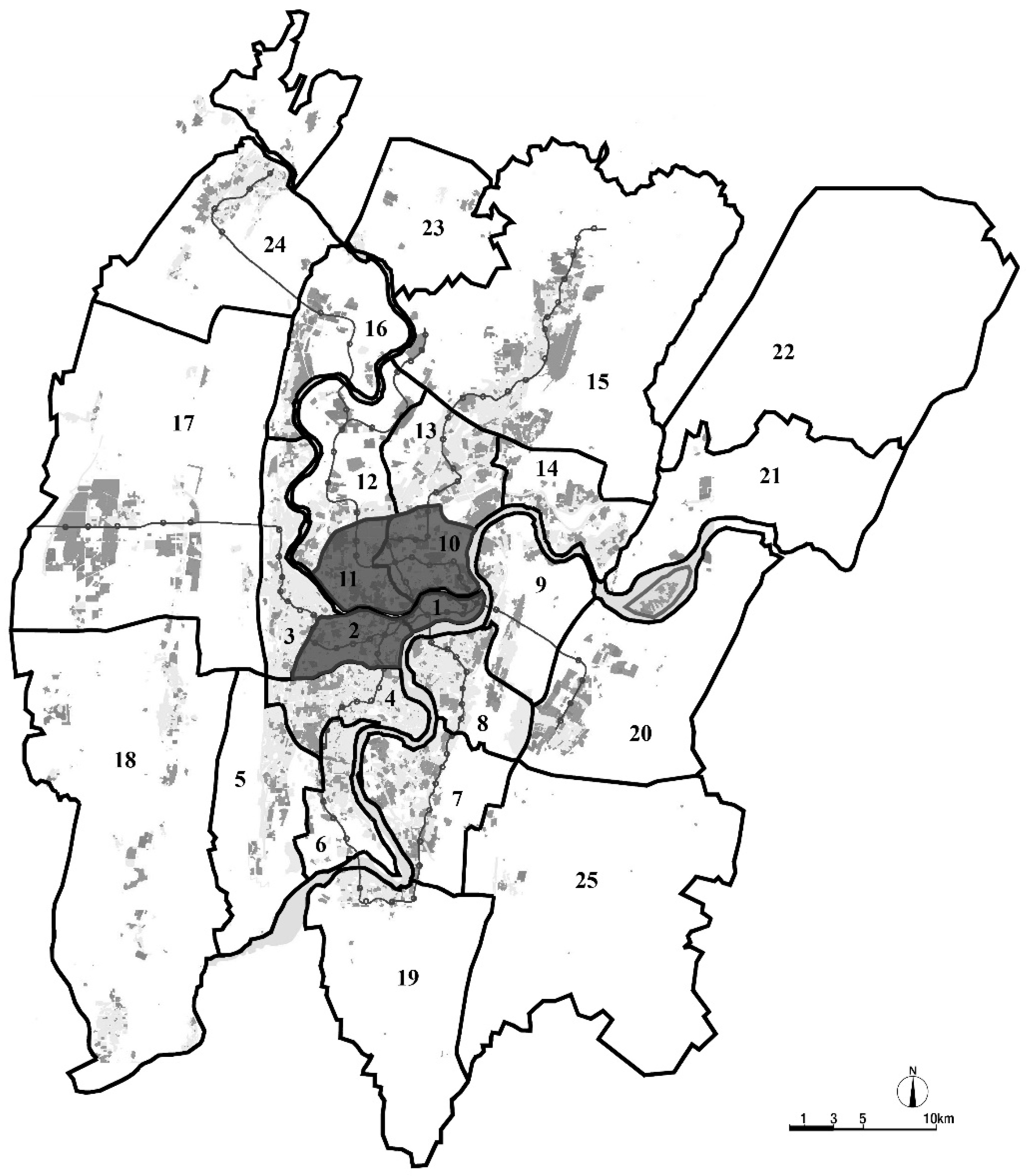
3.1. Data
3.1.1. Survey Method
3.1.2. Variables and Predictors
3.2. Modelling Approach
4. Results
4.1. Baseline Model
4.2. Model Comparison
4.3. Nonlinear Associations between Predictors and Travel Mode Choice
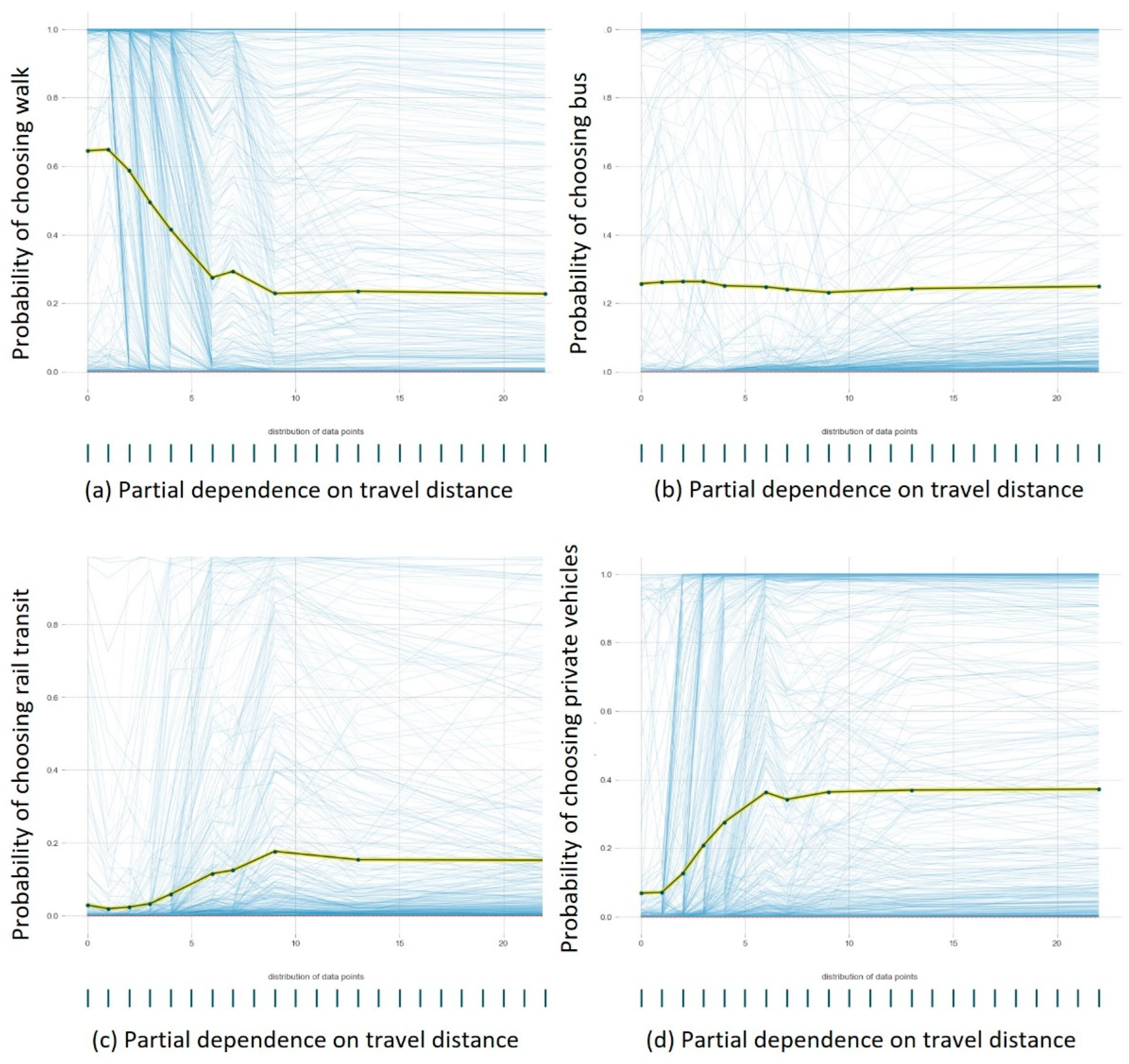
4.3.1. Trip Distance
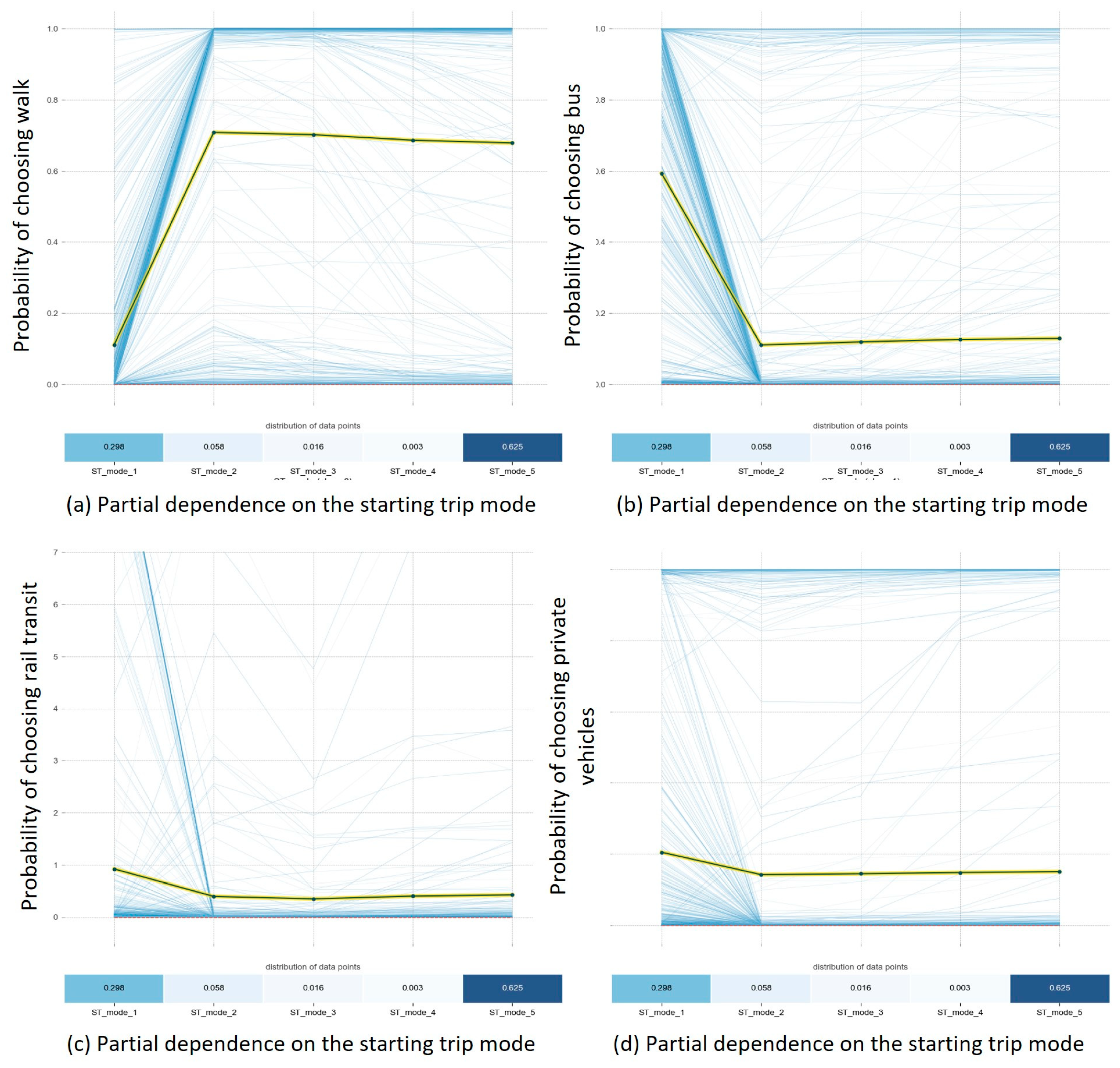
4.3.2. Travel Modes of the Starting Trip Stages
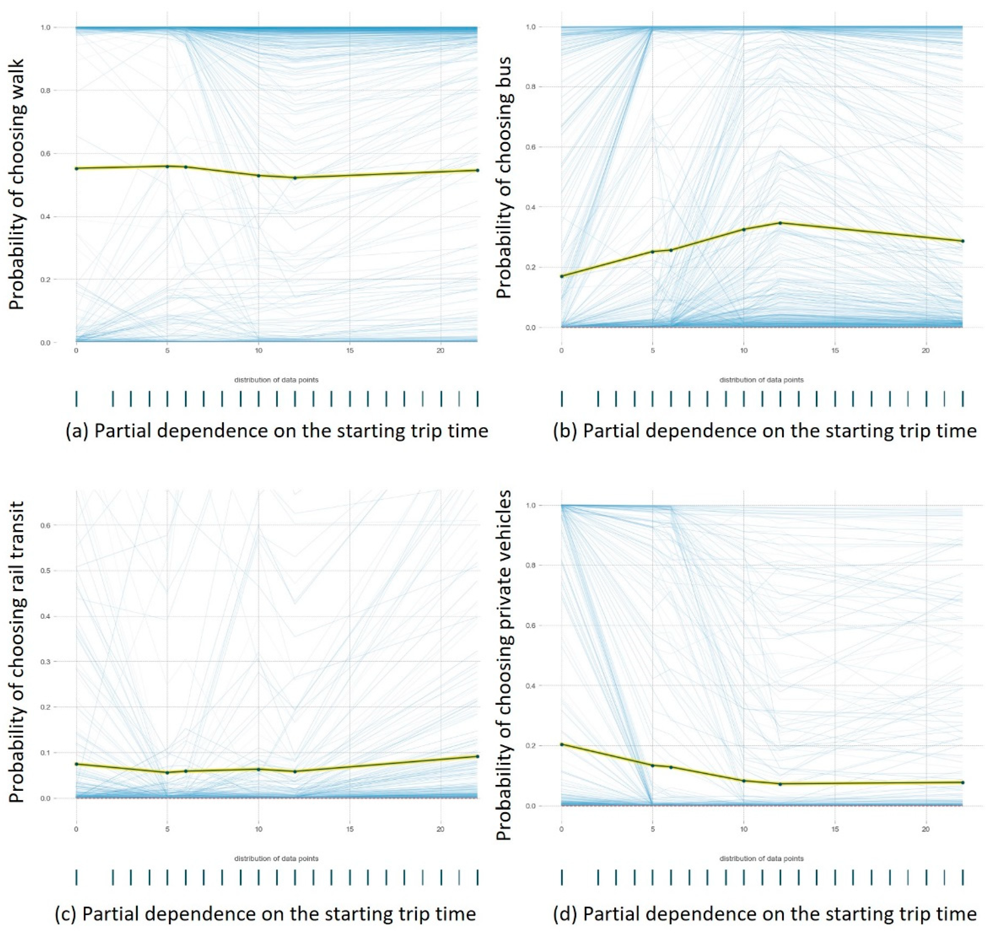
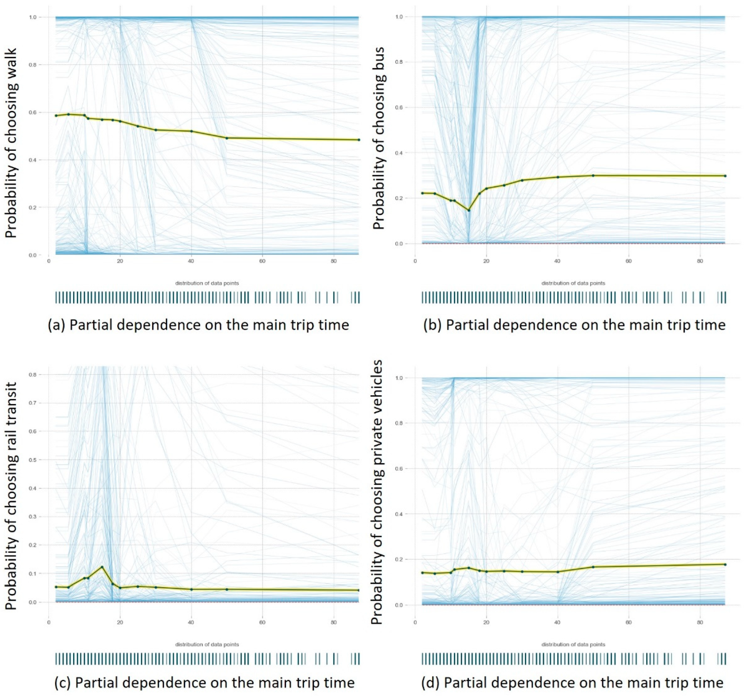
4.3.3. Duration of Different Trip Stages
4.4. Synergistic Effects between Variables
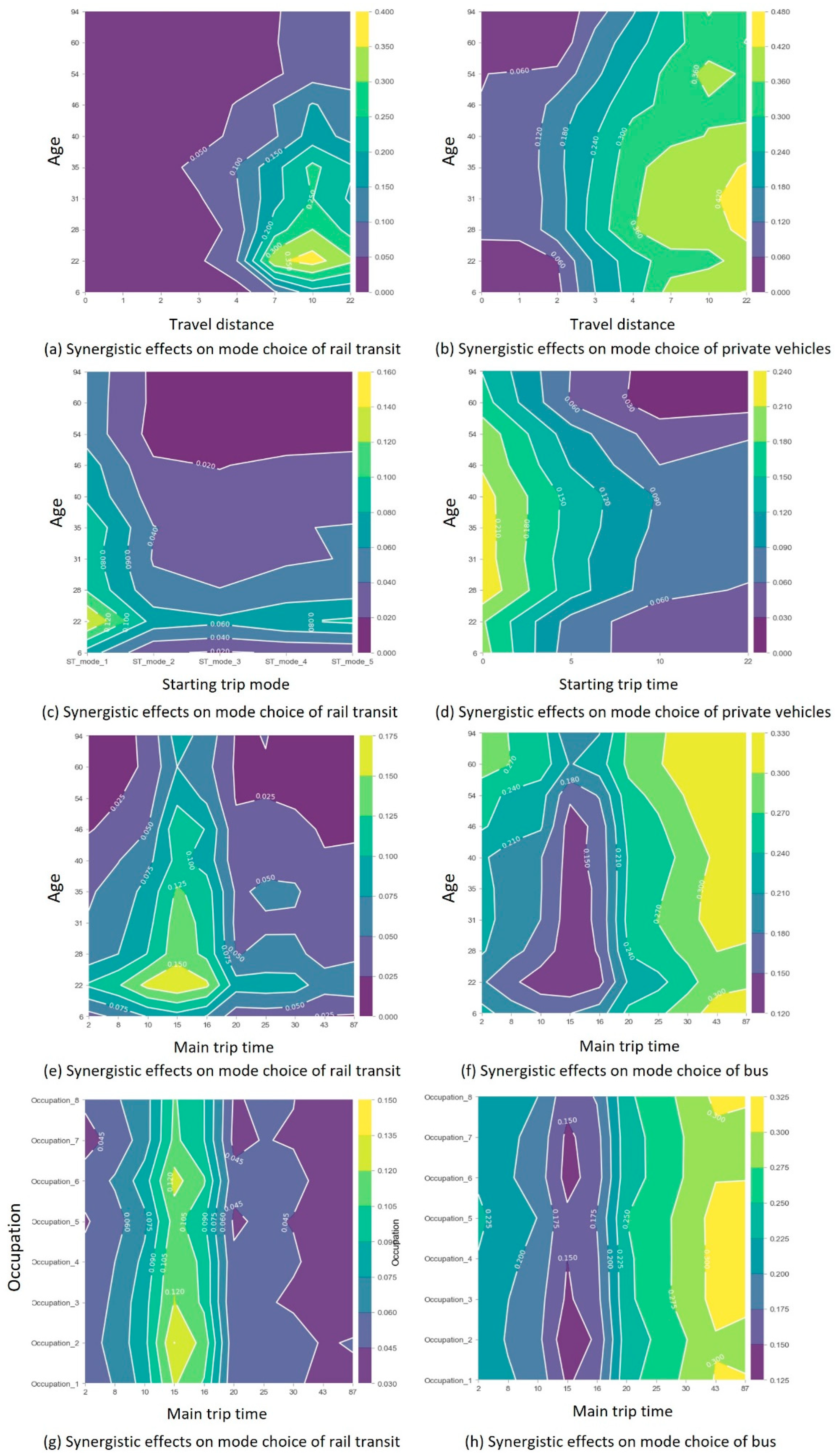
4.4.1. Synergistic Effects between Age and Trip Stage Characteristics
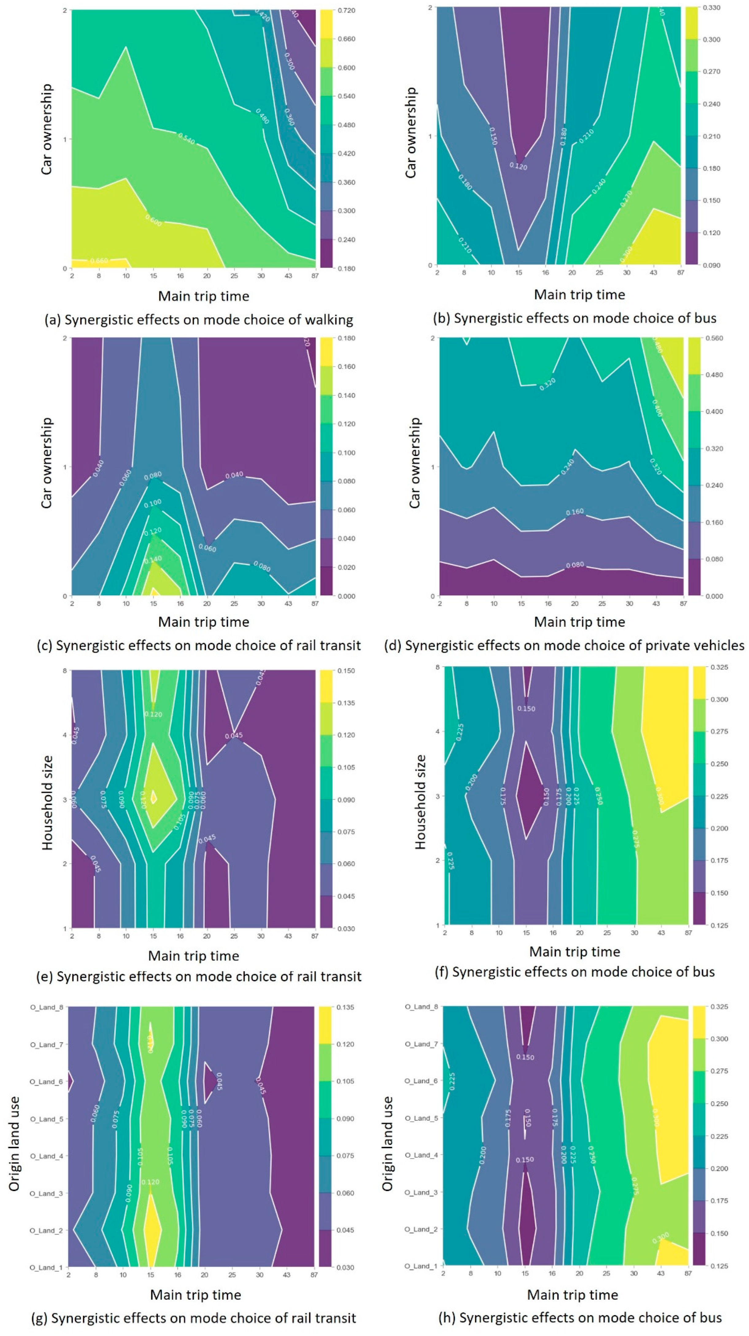
4.4.2. Synergistic Effects between Other Socio-Demographic Attributes and Trip Stage Characteristics
4.4.3. Synergistic Effects between Land Use and Trip Stage Characteristics
5. Conclusions
Author Contributions
Funding
Conflicts of Interest
References
- Dai, F.; Diao, M.; Sing, T.F. Effects of rail transit on individual travel mode shares: A two-dimensional propensity score matching approach. Transp. Res. Part D Transp. Environ. 2020, 89, 102601. [Google Scholar] [CrossRef]
- Luan, X.; Cheng, L.; Song, Y.; Zhao, J. Better understanding the choice of travel mode by urban residents: New insights from the catchment areas of rail transit stations. Sustain. Cities Soc. 2020, 53, 101968. [Google Scholar] [CrossRef]
- Molin, E.; Mokhtarian, P.; Kroesen, M. Multimodal travel groups and attitudes: A latent class cluster analysis of Dutch travelers. Transp. Res. Part A: Policy Pract. 2016, 83, 14–29. [Google Scholar] [CrossRef]
- Nobis, C. Multimodality: Facets and causes of sustainable mobility behavior. Transp. Res. Rec. 2007, 2010, 35–44. [Google Scholar] [CrossRef]
- Kuhnimhof, T.; Buehler, R.; Wirtz, M.; Kalinowska, D. Travel trends among young adults in Germany: Increasing multimodality and declining car use for men. J. Transp. Geogr. 2012, 24, 443–450. [Google Scholar] [CrossRef]
- Gadepalli, R.; Tiwari, G.; Bolia, N. Role of user’s socio-economic and travel characteristics in mode choice between city bus and informal transit services: Lessons from household surveys in Visakhapatnam, India. J. Transp. Geogr. 2020, 88, 102307. [Google Scholar] [CrossRef]
- Du, M.; Cheng, L.; Li, X.; Yang, J. Factors affecting the travel mode choice of the urban elderly in healthcare activity: Comparison between core area and suburban area. Sustain. Cities Soc. 2020, 52, 101868. [Google Scholar] [CrossRef]
- Dėdelė, A.; Miškinytė, A.; Andrušaitytė, S.; Nemaniūtė-Gužienė, J. Dependence between travel distance, individual socioeconomic and health-related characteristics, and the choice of the travel mode: A cross-sectional study for Kaunas, Lithuania. J. Transp. Geogr. 2020, 86, 102762. [Google Scholar] [CrossRef]
- Chen, X.; Guo, Y.; Yang, C.; Ding, F.; Yuan, Q. Exploring essential travel during COVID-19 quarantine: Evidence from China. Transp. Policy 2021, 111, 90–97. [Google Scholar] [CrossRef]
- Faber, R.M.; Jonkeren, O.; de Haas, M.C.; Molin, E.J.E.; Kroesen, M. Inferring modality styles by revealing mode choice heterogeneity in response to weather conditions. Transp. Res. Part A Policy Pract. 2022, 162, 282–295. [Google Scholar] [CrossRef]
- Deschaintres, E.; Morency, C.; Trépanier, M. Measuring Changes in Multimodal Travel Behavior Resulting from Transport Supply Improvement. Transp. Res. Rec. 2021, 2675, 533–546. [Google Scholar] [CrossRef]
- Klinger, T. Moving from monomodality to multimodality? Changes in mode choice of new residents. Transp. Res. Part A: Policy Pract. 2017, 104, 221–237. [Google Scholar] [CrossRef]
- Duca, G.; Trincone, B.; Bagamanova, M.; Meincke, P.; Russo, R.; Sangermano, V. Passenger Dimensions in Sustainable Multimodal Mobility Services. Sustainability 2022, 14, 12254. [Google Scholar] [CrossRef]
- Oostendorp, R.; Gebhardt, L. Combining means of transport as a users’ strategy to optimize traveling in an urban context: Empirical results on intermodal travel behavior from a survey in Berlin. J. Transp. Geogr. 2018, 71, 72–83. [Google Scholar] [CrossRef]
- An, Z.; Heinen, E.; Watling, D. The level and determinants of multimodal travel behavior: Does trip purpose make a difference? Int. J. Sustain. Transp. 2023, 17, 103–117. [Google Scholar] [CrossRef]
- Scheiner, J.; Chatterjee, K.; Heinen, E. Key events and multimodality: A life course approach. Transp. Res. Part A Policy Pract. 2016, 91, 148–165. [Google Scholar] [CrossRef]
- Heinen, E. Are multimodals more likely to change their travel behaviour? A cross-sectional analysis to explore the theoretical link between multimodality and the intention to change mode choice. Transp. Res. Part F Traffic Psychol. Behav. 2018, 56, 200–214. [Google Scholar] [CrossRef]
- Olafsson, A.S.; Nielsen, T.S.; Carstensen, T.A. Cycling in multimodal transport behaviours: Exploring modality styles in the Danish population. J. Transp. Geogr. 2016, 52, 123–130. [Google Scholar] [CrossRef]
- Heinen, E.; Mattioli, G. Does a high level of multimodality mean less car use? An exploration of multimodality trends in England. Transportation 2019, 46, 1093–1126. [Google Scholar] [CrossRef]
- Heinen, E.; Chatterjee, K. The same mode again? An exploration of mode choice variability in Great Britain using the National Travel Survey. Transp. Res. Part A Policy Pract. 2015, 78, 266–282. [Google Scholar] [CrossRef]
- Diana, M.; Pirra, M. A comparative assessment of synthetic indices to measure multimodality behaviours. Transp. A Transp. Sci. 2016, 12, 771–793. [Google Scholar] [CrossRef]
- Heinen, E.; Mattioli, G. Multimodality and CO2 emissions: A relationship moderated by distance. Transp. Res. Part D Transp. Environ. 2019, 75, 179–196. [Google Scholar] [CrossRef]
- MoT. 12th Five-Year Plan for Transportation; Ministry of Transport of the People’s Republic of China: Bejing, 2011.
- Kirtonia, S.; Sun, Y. Evaluating rail transit’s comparative advantages in travel cost and time over taxi with open data in two U.S. cities. Transp. Policy 2022, 115, 75–87. [Google Scholar] [CrossRef]
- Haustein, S.; Siren, A. Older people’s mobility: Segments, factors, trends. Transp. Rev. 2015, 35, 466–487. [Google Scholar] [CrossRef]
- Buehler, R.; Hamre, A. The multimodal majority? Driving, walking, cycling, and public transportation use among American adults. Transportation 2015, 42, 1081–1101. [Google Scholar] [CrossRef]
- Kroesen, M. Modeling the behavioral determinants of travel behavior: An application of latent transition analysis. Transp. Res. Part A Policy Pract. 2014, 65, 56–67. [Google Scholar] [CrossRef]
- Li, S.; Lyu, D.; Huang, G.; Zhang, X.; Gao, F.; Chen, Y.; Liu, X. Spatially varying impacts of built environment factors on rail transit ridership at station level: A case study in Guangzhou, China. J. Transp. Geogr. 2020, 82, 102631. [Google Scholar] [CrossRef]
- Zhou, M.; Wang, D.; Guan, X. Co-evolution of the built environment and travel behaviour in Shenzhen, China. Transp. Res. Part D Transp. Environ. 2022, 107, 103291. [Google Scholar] [CrossRef]
- Bautista-Hernández, D.A. Mode choice in commuting and the built environment in México City. Is there a chance for non-motorized travel? J. Transp. Geogr. 2021, 92, 103024. [Google Scholar] [CrossRef]
- Blumenberg, E.; Pierce, G. Multimodal travel and the poor: Evidence from the 2009 National Household Travel Survey. Transp. Lett. 2014, 6, 36–45. [Google Scholar] [CrossRef]
- McLaren, A.T. Families and transportation: Moving towards multimodality and altermobility? J. Transp. Geogr. 2016, 51, 218–225. [Google Scholar] [CrossRef]
- Zhao, J.; Fan, W.; Zhai, X. Identification of land-use characteristics using bicycle sharing data: A deep learning approach. J. Transp. Geogr. 2020, 82, 102562. [Google Scholar] [CrossRef]
- Tao, T.; Cao, J. Examining motivations for owning autonomous vehicles: Implications for land use and transportation. J. Transp. Geogr. 2022, 102, 103361. [Google Scholar] [CrossRef]
- Cheng, L.; Yang, J.; Chen, X.; Cao, M.; Zhou, H.; Sun, Y. How could the station-based bike sharing system and the free-floating bike sharing system be coordinated? J. Transp. Geogr. 2020, 89, 102896. [Google Scholar] [CrossRef]
- Bai, S.; Jiao, J. Using Deep Learning to Understand Travel Demands in Different Urban Districts. Transp. Res. Rec. 2021, 2675, 117–128. [Google Scholar] [CrossRef]
- Cheng, L.; Wang, K.; De Vos, J.; Huang, J.; Witlox, F. Exploring non-linear built environment effects on the integration of free-floating bike-share and urban rail transport: A quantile regression approach. Transp. Res. Part A Policy Pract. 2022, 162, 175–187. [Google Scholar] [CrossRef]
- Xie, C.; Lu, J.; Parkany, E. Work travel mode choice modeling with data mining: Decision trees and neural networks. Transp. Res. Rec. 2003, 1854, 50–61. [Google Scholar] [CrossRef]
- Zhao, X.; Yan, X.; Yu, A.; Van Hentenryck, P. Prediction and behavioral analysis of travel mode choice: A comparison of machine learning and logit models. Travel Behav. Soc. 2020, 20, 22–35. [Google Scholar] [CrossRef]
- Cheng, L.; De Vos, J.; Zhao, P.; Yang, M.; Witlox, F. Examining non-linear built environment effects on elderly’s walking: A random forest approach. Transp. Res. Part D Transp. Environ. 2020, 88, 102552. [Google Scholar] [CrossRef]
- Liu, J.; Wang, B.; Xiao, L. Non-linear associations between built environment and active travel for working and shopping: An extreme gradient boosting approach. J. Transp. Geogr. 2021, 92, 103034. [Google Scholar] [CrossRef]
- Frank, L.D.; Pivo, G. Impacts of mixed use and density on utilization of three modes of travel: Single-occupant vehicle, transit, and walking. Transp. Res. Rec. 1994, 1466, 44–52. [Google Scholar]
- Ding, C.; Cao, X.; Liu, C. How does the station-area built environment influence Metrorail ridership? Using gradient boosting decision trees to identify non-linear thresholds. J. Transp. Geogr. 2019, 77, 70–78. [Google Scholar] [CrossRef]
- Ding, C.; Cao, X.; Næss, P. Applying gradient boosting decision trees to examine non-linear effects of the built environment on driving distance in Oslo. Transp. Res. Part A Policy Pract. 2018, 110, 107–117. [Google Scholar] [CrossRef]
- Szaruga, E.; Załoga, E. Sustainable Development Programming of Airports by Identification of Non-Efficient Units. Energies 2022, 15, 932. [Google Scholar] [CrossRef]
- Yue, M.; Ma, S. LSTM-Based Transformer for Transfer Passenger Flow Forecasting between Transportation Integrated Hubs in Urban Agglomeration. Appl. Sci. 2023, 13, 637. [Google Scholar] [CrossRef]
- Slinker, B.; Glantz, S. Multiple regression for physiological data analysis: The problem of multicollinearity. Am. J. Physiol.-Regul. Integr. Comp. Physiol. 1985, 249, R1–R12. [Google Scholar] [CrossRef]
- Abdelsalam, O.; El-Masry, A.; Elsegini, S. Board composition, ownership structure and dividend policies in an emerging market: Further evidence from CASE 50. Manag. Financ. 2008, 34, 953–964. [Google Scholar]
- Grubbs, F.E. Procedures for detecting outlying observations in samples. Technometrics 1969, 11, 1–21. [Google Scholar] [CrossRef]
- Yin, C.; Cao, J.; Sun, B.; Liu, J. Exploring built environment correlates of walking for different purposes: Evidence for substitution. J. Transp. Geogr. 2023, 106, 103505. [Google Scholar] [CrossRef]
- Lhéritier, A.; Bocamazo, M.; Delahaye, T.; Acuna-Agost, R. Airline itinerary choice modeling using machine learning. J. Choice Model. 2019, 31, 198–209. [Google Scholar] [CrossRef]
- Chen, T.; Guestrin, C. Xgboost: A scalable tree boosting system. In Proceedings of the 22nd acm sigkdd international conference on knowledge discovery and data mining, San Francisco, CA, USA, 13–17 August 2016; pp. 785–794. [Google Scholar]
- Friedman, J.H. Greedy function approximation: A gradient boosting machine. Ann. Stat. 2001, 29, 1189–1232. [Google Scholar] [CrossRef]
- Goldstein, A.; Kapelner, A.; Bleich, J.; Pitkin, E. Peeking inside the black box: Visualizing statistical learning with plots of individual conditional expectation. J. Comput. Graph. Stat. 2015, 24, 44–65. [Google Scholar] [CrossRef]
- Greenwell, B.M.; Boehmke, B.C.; McCarthy, A.J. A Simple and Effective Model-Based Variable Importance Measure. arXiv 2018, arXiv:1805.04755. [Google Scholar] [CrossRef]
- Karhade, A.V.; Schwab, J.H.; Bedair, H.S. Development of machine learning algorithms for prediction of sustained postoperative opioid prescriptions after total hip arthroplasty. J. Arthroplast. 2019, 34, 2272–2277. [Google Scholar] [CrossRef]
- Ghosh, S.M.; Behera, M.D. Aboveground biomass estimates of tropical mangrove forest using Sentinel-1 SAR coherence data-The superiority of deep learning over a semi-empirical model. Comput. Geosci. 2021, 150, 104737. [Google Scholar] [CrossRef]
- Liu, L.; Dennett, A.; Hickman, R. Social equity impacts of rail transit investments using community perceptions: Evidence from Chongqing. Transp. Plan. Technol. 2023, 46, 1–21. [Google Scholar] [CrossRef]
- Becker, H.; Ciari, F.; Axhausen, K.W. Measuring the car ownership impact of free-floating car-sharing–A case study in Basel, Switzerland. Transp. Res. Part D: Transp. Environ. 2018, 65, 51–62. [Google Scholar] [CrossRef]


| Variable | Description | Category | % | Min | Max | Mean | SD |
|---|---|---|---|---|---|---|---|
| Dependent Variable | |||||||
| MA_mode | Travel mode of the main trip | 0 = walk | 55.2% | ||||
| 1 = bus | 23.6% | ||||||
| 2 = rail transit | 6.2% | ||||||
| 3 = private vehicles | 15.0% | ||||||
| Independent Variables | |||||||
| Trip characteristics | |||||||
| TT | Travel time of the whole trip (min) | 2 | 630 | 31.9 | 22.3 | ||
| MA_time | Travel time of the main trip (min) | 2 | 240 | 22.4 | 15.6 | ||
| ST_time | Travel time of the starting trip (min) | 0 | 60 | 3.1 | 5.0 | ||
| ED_time | Travel time of the ending trip (min) | 0 | 44 | 1.7 | 3.9 | ||
| TD | Distance between the start point and the ending point of an outbound journey, based on the road network in the city (km) | 0 | 61 | 4.4 | 5.9 | ||
| ST_mode | Travel mode of the starting trip | 0 = walk | 30.1% | ||||
| 1 = bus | 5.9% | ||||||
| 2 = rail transit | 1.7% | ||||||
| 3 = private vehicles | 0.3% | ||||||
| 4 = vacant | 62.1% | ||||||
| ED_mode | Travel mode of the ending trip | 0 = walk | 19.0% | ||||
| 1 = bus | 1.8% | ||||||
| 2 = rail transit | 0.8% | ||||||
| 3 = private vehicles | 0.1% | ||||||
| 4 = vacant | 78.4% | ||||||
| ST_ct | Starting time categories | 1 = before 10:00 am, | 40.7% | ||||
| 2 = 10:00 am-12:00 am | 7.9% | ||||||
| 3 = 12:00 am-15:00 pm | 10.7% | ||||||
| 4 = 15:00 am-18:00 pm | 20.1% | ||||||
| 5 = after 18:00 pm | 20.5% | ||||||
| AR_category | Arriving time categories | 1 = before 10:00 am, | 38.9% | ||||
| 2 = 10:00 am-12:00 am | 8.4% | ||||||
| 3 = 12:00 am-15:00 pm | 11.5% | ||||||
| 4 = 15:00 am-18:00 pm | 14.0% | ||||||
| 5 = after 18:00 pm | 27.1% | ||||||
| TP | Trip purpose | 1 = go back home | 43.4% | ||||
| 2 = commute to work | 30.6% | ||||||
| 3 = go to school | 4.7% | ||||||
| 4 = visiting friends, dining, recreation, shopping etc. | 18.4% | ||||||
| 5 = go to hospital | 0.6% | ||||||
| 6 = others | 2.3% | ||||||
| Socio-demographic attributes | |||||||
| Age | Age of the respondent in years | 6 | 94 | 39.30 | 15.64 | ||
| H_size | Number of members in the respondent’s household | 1 | 8 | 3.11 | 0.95 | ||
| Child_No | Number of young child (below 18) in the respondent’s household | 0 | 2 | 0.21 | 0.42 | ||
| Car_own | Number of household -owned cars | 0 | 2 | 0.33 | 0.52 | ||
| Gender | 1 = male | 47.6% | |||||
| 2 = female | 52.4% | ||||||
| Occupation | 1 = student | 9.5% | |||||
| 2 = company employees | 25.3% | ||||||
| 3 = service staff | 15.6% | ||||||
| 4 = civil servant | 7.9% | ||||||
| 5 = industrial workers | 4.9% | ||||||
| 6 = retired people | 16.9% | ||||||
| 7 = free-lanced workers | 11.3% | ||||||
| 8 = others | 8.6% | ||||||
| Hukou | 1 = local hukou holders | 73.3% | |||||
| 2 = outbound resident who do not have local hukou | 26.7% | ||||||
| Car_plan | Household car consumption plan | 1 = plan to buy car before 2015 | 5.5% | ||||
| 2 = plan to buy cars between 2016 and 2020 (five years after the rail transit system established) | 25.5% | ||||||
| 3 = no plan to buy cars before 2020 | 69.0% | ||||||
| Parking | Whether or not respondent’s household has a parking place of their own | 1 = no | 69.5% | ||||
| 2 = yes | 30.5% | ||||||
| RP_level | Including upscale new residential buildings, town houses, and villas | 1 = poor condition/old properties/public rental properties | 22.8% | ||||
| 2 = ordinary properties/gated communities | 74.9% | ||||||
| 3 = luxury properties | 2.3% | ||||||
| Build environment elements | |||||||
| O_land | Origin land use coding | 1 = residential land | 45.3% | ||||
| D_land | Destination land coding | 2 = office land | 12.7% | ||||
| 3 = commercial land | 17.8% | ||||||
| 4 = education land | 7.6% | ||||||
| 5 = hospital land | 1.5% | ||||||
| 6 = industrial and storage land | 2.1% | ||||||
| 7 = transportation land | 0.5% | ||||||
| 8 = others | 12.5% | ||||||
| Effect | Likelihood Ratio | ||
|---|---|---|---|
| Chi-Square | df | Sig. | |
| Constant | 0.00 | 0 | |
| TD | 985.73 | 3 | 0.000 |
| ST_mode | 4417.19 | 12 | 0.000 |
| ST_time | 121.09 | 3 | 0.000 |
| MA_time | 223.97 | 3 | 0.000 |
| TT | 12.57 | 3 | 0.006 |
| ED_time | 18.65 | 3 | 0.000 |
| ED_mode | 545.85 | 12 | 0.000 |
| ST_ct | 47.10 | 12 | 0.000 |
| TP | 29.43 | 15 | 0.014 |
| Car_own | 1212.12 | 3 | 0.000 |
| Age | 378,193.07 | 3 | 0.000 |
| Gender | 151.24 | 3 | 0.000 |
| H_size | 41.17 | 3 | 0.000 |
| Occupation | 148.50 | 21 | 0.000 |
| Child_No | 23.21 | 3 | 0.000 |
| Hukou | 19.83 | 3 | 0.000 |
| RP_level | 11.30 | 6 | 0.079 |
| Car_plan | 11.19 | 6 | 0.083 |
| D_land | 63.14 | 21 | 0.000 |
| O_land | 61.69 | 21 | 0.000 |
| Predictor Variables | XGBT | Random Forest | Decision Tree | AdaBoost | Logistic Regression | |||||
|---|---|---|---|---|---|---|---|---|---|---|
| RI | Rank | RI | Rank | RI | Rank | RI | Rank | RI | Rank | |
| Trip characteristics | ||||||||||
| TD | 26.56% | 1 | 20.17% | 2 | 20.80% | 1 | 5.23% | 6 | 16.39% | 2 |
| ST_mode | 21.18% | 2 | 20.81% | 1 | 19.92% | 2 | 12.99% | 4 | 15.22% | 3 |
| ST_time | 10.05% | 4 | 8.06% | 5 | 9.61% | 5 | 0.79% | 13 | 6.67% | 5 |
| MA_time | 8.59% | 5 | 8.58% | 4 | 8.00% | 6 | 17.87% | 2 | 11.38% | 4 |
| TT | 2.61% | 7 | 4.76% | 6 | 14.03% | 4 | 2.01% | 9 | 2.39% | 11 |
| ED_time | 2.60% | 8 | 4.09% | 7 | 6.32% | 7 | 2.73% | 8 | 4.08% | 7 |
| ED_mode | 1.95% | 9 | 3.29% | 8 | 0.76% | 10 | 12.00% | 5 | 4.12% | 6 |
| ST_ct | 0.56% | 13 | 1.00% | 16 | 0.25% | 12 | 0.49% | 15 | 1.22% | 16 |
| TT | 0.13% | 19 | 0.99% | 17 | 0.00% | 18 | 0.26% | 18 | 1.48% | 15 |
| Socio-demographic attributes | ||||||||||
| Car_own | 17.35% | 3 | 15.57% | 3 | 14.21% | 3 | 4.07% | 7 | 19.53% | 1 |
| Age | 4.58% | 6 | 2.95% | 9 | 4.40% | 8 | 18.35% | 1 | 2.82% | 8 |
| Gender | 0.90% | 10 | 1.34% | 12 | 0.00% | 20 | 0.27% | 17 | 1.09% | 17 |
| H_size | 0.71% | 11 | 0.84% | 18 | 0.00% | 16 | 17.23% | 3 | 2.49% | 10 |
| Occupation | 0.60% | 12 | 1.62% | 11 | 1.01% | 9 | 1.60% | 11 | 2.36% | 12 |
| Child_No | 0.55% | 14 | 1.64% | 10 | 0.00% | 17 | 0.00% | 19 | 2.78% | 9 |
| Hukou | 0.23% | 17 | 0.50% | 19 | 0.02% | 15 | 0.27% | 16 | 0.46% | 20 |
| RP_level | 0.16% | 18 | 1.03% | 15 | 0.53% | 11 | 0.00% | 20 | 0.55% | 18 |
| Car_plan | 0.11% | 20 | 0.36% | 20 | 0.07% | 14 | 0.63% | 14 | 0.47% | 19 |
| Build environment elements | ||||||||||
| D_land | 0.32% | 15 | 1.32% | 13 | 0.00% | 19 | 1.44% | 12 | 2.18% | 14 |
| O_land | 0.24% | 16 | 1.09% | 14 | 0.08% | 13 | 1.78% | 10 | 2.31% | 13 |
| F1 score | 0.848 | 0.791 | 0.753 | 0.726 | 0.696 | |||||
| Recall | 0.829 | 0.762 | 0.744 | 0.721 | 0.684 | |||||
| Precision | 0.874 | 0.858 | 0.772 | 0.733 | 0.757 | |||||
Disclaimer/Publisher’s Note: The statements, opinions and data contained in all publications are solely those of the individual author(s) and contributor(s) and not of MDPI and/or the editor(s). MDPI and/or the editor(s) disclaim responsibility for any injury to people or property resulting from any ideas, methods, instructions or products referred to in the content. |
© 2023 by the authors. Licensee MDPI, Basel, Switzerland. This article is an open access article distributed under the terms and conditions of the Creative Commons Attribution (CC BY) license (https://creativecommons.org/licenses/by/4.0/).
Share and Cite
Liu, L.; Wang, Y.; Hickman, R. How Rail Transit Makes a Difference in People’s Multimodal Travel Behaviours: An Analysis with the XGBoost Method. Land 2023, 12, 675. https://doi.org/10.3390/land12030675
Liu L, Wang Y, Hickman R. How Rail Transit Makes a Difference in People’s Multimodal Travel Behaviours: An Analysis with the XGBoost Method. Land. 2023; 12(3):675. https://doi.org/10.3390/land12030675
Chicago/Turabian StyleLiu, Lixun, Yujiang Wang, and Robin Hickman. 2023. "How Rail Transit Makes a Difference in People’s Multimodal Travel Behaviours: An Analysis with the XGBoost Method" Land 12, no. 3: 675. https://doi.org/10.3390/land12030675