The Extension of Vegetable Production to High Altitudes Increases the Environmental Cost and Decreases Economic Benefits in Subtropical Regions

Abstract

Global warming has driven the expansion of cultivated land to high-altitude areas. Intensive vegetable production, which is generally considered to be a high economic value and high environmental risk system, has expanded greatly in high-altitude mountainous areas of China. However, the environmental cost of vegetable production in these areas is poorly understood. In this study, pepper production at low (traditional pepper production area) and high (newly expanded area) altitudes were investigated in Shizhu, a typical pepper crop area. The output and environmental cost at the two altitudes were identified. the influence of resource inputs, climate, and soil properties on pepper production was evaluated. There were obvious differences in output and environmental cost between the two altitudes. High-altitude pepper production achieved a 16.2% lower yield, and had a higher fertilizer input, resulting in a 22.3% lower net ecosystem economic benefit (NEEB), 23.0% higher nitrogen (N) footprint and 24.0% higher carbon (C) footprint compared to low-altitude farming. There is potential for environmental mitigation with both high- and low-altitude pepper production; Compared to average farmers, high-yield farmers groups reduced their N and C footprints by 16.9–24.8% and 18.3–25.2%, respectively, with 30.6–34.1% higher yield. A large increase in yield could also be achieved by increasing the top-dress fertilizer rate and decreasing the plant density. Importantly, high-altitude pepper production was achieved despite less advanced technology and inferior conditions (e.g., a poor road system and uneven fields). It provides a reference for the study of the environmental cost of other high-altitude regions or other crop systems at high-altitude areas.

1. Introduction

The global warming-driven expansion of cultivated land to high altitudes [1,2] has resulted in mountainous areas becoming an important source of vegetables and other agricultural products. To obtain a high yield and maximize economic benefits, excessive nitrogen (N) fertilizer (>350 kg ha⁻¹ season⁻¹), among other inputs, is commonly applied in high-altitude vegetable production [3]. This excessive fertilizer input imposes a significant environmental burden [4,5,6]. Thus, the environmental cost of vegetable production at high altitudes needs to be evaluated to facilitate sustainable vegetable production.

Substantial research has been conducted on the environmental cost of various crop production systems and cultivation patterns (e.g., open field vs. greenhouse, organic farming vs. conventional farming), among other factors (e.g., domestic vs. imported products) [7,8]. However, most of these studies were conducted in low-altitude regions (<1000 m), and the environmental cost of vegetable production at high altitudes remains unclear. There are large differences in climate, soil properties, and farm management practices between high- and low-altitude areas, which may have significant effects on yield and environmental cost. Carbon (C) and N footprints, which are quantified as the reactive N and CO₂-equivalent (CO₂-eq) emissions per unit weight of product through life cycle assessment (LCA), can be used to assess the sustainability of agricultural systems and detect greenhouse gas (GHG) and reactive nitrogen (Nr) emission hotspots in the food production system [9,10]. However, most farmers focus predominantly on economic returns. Estimation of the net ecosystem economic benefit (NEEB) is useful for striking a balance between the economic benefits of grain yield and the environmental costs of C emissions and N loss [9,11]. High-altitude vegetable production enables residents of mountainous areas to overcome poverty by obtaining more income via the expansion of the scale of local agricultural activities. Thus, it is important to compare economic benefits and environmental costs between high- and low-altitude vegetable production areas, with consideration of the yield gap. This could lead to new methods for increasing yield and achieving environmental mitigation [12].

Increasing crop yield while simultaneously reducing the environmental cost of agriculture is one of the greatest barriers to a sustainable agricultural production system [13,14]. Large differences exist in yields among small-hold farmers due to variations in management practices. For example, a high-yield group (top 50%) obtained 59.3% more pepper than a low-yield group (bottom 50%) [15]. Other studies [16,17] have suggested that the yield gap can be significantly closed by optimizing nutrient and crop management. For example, the pepper yield was increased by 26.7% by adopting “best practice” farming methods [18]. The environmental cost differs among farmers according to crop management [19,20]. Understanding the relationship between yield and environmental cost for specific regions and crop systems is important for the development of feasible mitigation measures.

Previous studies [17,18] suggested that closing the yield gap could reduce the C footprint by 23.9–51.2%, which could be achieved by applying best-practice nutrient and crop management methods in intensive vegetable production systems. However, the environmental mitigation potential of vegetable production systems at high altitudes remains poorly understood, and the relationship between yield and environmental cost is still unclear. If vegetable production continues to extend at high altitudes, the environmental cost may increase, and NEEB will decrease in subtropical regions, then closing the yield gap could mitigate the environmental cost and raise the NEEB. Pepper (Capsicum annuum L.) is the most extensively grown vegetable species in China, in terms of planting area [18]. China accounts for 50.8% of pepper production worldwide (FAO, 2013). Southwest China is the major pepper production and consumption area. The objectives of this study were to: compare the differences in resource input, yield, NEEB, and N and C emission between high- and low-altitude pepper production areas; determine the potential of yield increase and environmental cost reduction of high-altitude pepper production; and identify optimal management practices.

2. Materials and Methods

2.1. Study Area and Data Sources

We conducted a survey in Shizhu County (118°04′–118°29′ E; 31°22′–32°03′ N), Chongqing Province, a typical open-field pepper production area in China. Pepper grown in this area is mainly used in condiments. Pepper production is a major industry in Shizhu County, with the planting area increasing by 21.2% during the period 2010–2017. The expansion of production to high altitudes has been an important factor in this increase. Shizhu County is a humid region with a monsoon climate. The average rainfall is 1200 mm/year. Sixty farmers were randomly selected for face-to-face interviews. The farmers were from high altitude levels (HAL, 900–1200 m; pepper growth period = April to July, monthly air temperature = 18.4 °C, average monthly rainfall = 136.9 mm) and low altitude level (LAL; 500–800 m); pepper growth period = March to June, average monthly air temperature = 22.7 °C, average monthly rainfall = 138.2 mm) areas (

Table 1. The climate during the growth stage, soil property and plant density of open-field pepper production in HAL and LAL. HAL represents the high-elevation level (500–800 m), and LAL represents the low-altitude level (900–1200 m).

		Unit	HAL	LAL
Climate during growth stage	Monthly temperature	℃	18.6	22.7
	Monthly precipitation	mm	139.5	144.8
Soil property	pH		5.3 ± 1.0	6.1 ± 1.3
	Organic matter	g kg−1	21.2 ± 18.6	13.4 ± 5.8
	Available N	mg kg−1	103.9 ± 28.4	89.2 ± 33
	Available P	mg kg−1	11.0 ± 9.1	12.8 ± 11.3
	Available K	mg kg−1	104.6 ± 43.7	73.1 ± 40.7
Cultivated land	Surface slope	Degree (°)	13.1 ± 4.6	9.8 ± 6.4
Plant density		103 plant ha−1	41.5 ± 8.4	43.9 ± 8.9

The value represented the mean ± standard deviation (SD).

). We also interviewed two dealers selling seeds, fertilizers, pesticides, and plastic film.

The data collected from the interviews included the transplanting date, planting area, pepper yield, planting density, fertilization date, and growth period, and the application rate of resource inputs (including fertilizers, pesticides, plastic film, and the diesel consumed by agricultural machines). Soil property data were obtained from the Soil Testing and Fertilizer Recommendation Program, which was implemented in the study region during the period 2010–2016; 106 samples were obtained from high altitudes and 170 from low altitudes.

2.2. System Boundary

The Nr and GHG emissions for open-field pepper production were analyzed through an LCA (from cradle to grave). The study focused on vegetable production and its system boundaries; the agricultural materials stage (MS) and arable farming stage (FS) were distinguished. The MS included the production and transport of agricultural materials applied during pepper production (inorganic fertilizer, organic fertilizer, pesticides, plastic film, and diesel consumed by agricultural machines). The impact of seeds was not considered because only small quantities were used. The FS involved the application of each agricultural input (inorganic fertilizer, organic fertilizer, pesticide, and diesel). To determine the environmental and economic impacts, we expressed the results in the following units: per ha, per ton of fresh peppers produced, and in terms of NEEB (i.e., CNY Yuan).

2.3. Reactive Nitrogen Emissions

The Nr emissions (kg N ha⁻¹) were calculated using the following equation:

$$Nr emission={\Sigma }_{i=1}^{m}M{S}_{i_{\mathrm{N}\mathrm{r}}}+{\Sigma }_{j=1}^{n}F{S}_{j_{\mathrm{N}\mathrm{r}}}$$

where MS_iNr represents Nr emissions during the MS, including from the production and transportation of fertilizer, pesticides, plastic film, and diesel consumed by agricultural machines (calculated by multiplying their application rate by relevant emission factors). We used the most local and recent indicators for each emission factor. The relative quantities of pollutants emitted from fertilizers, pesticides, diesel, and plastic at the MS are listed in Table S1. The term FS_jNr represents Nr emission from inorganic and organic N fertilizer following their application to a vegetable field (FS), including nitrous oxide (N₂O) emissions, ammonia (NH₃) volatilization, and N leaching and runoff. The details of the emission factors of the various Nr species are given in Table S2.

2.4. Greenhouse Gas Emissions

The GHG emissions (kg N ha⁻¹) were determined by the following equation:

$$GHG emission={\Sigma }_{i=1}^{m}M{S}_{i_{{\mathrm{C}\mathrm{O}}_2}}+{\Sigma }_{j=1}^{n}F{S}_{j_{{\mathrm{C}\mathrm{O}}_2}}$$

where MS_iCO₂ represents the emissions during the MS, including the production and transport of agricultural materials (inorganic fertilizer, organic fertilizer, pesticides, plastic film, and diesel consumed by agricultural machines). The term FSjCO₂ represents the GHG emissions from the FS for the inputs (inorganic fertilizer, organic fertilizer, pesticides, plastic film, and diesel consumed by agricultural machines). We applied an approach from the literature based on crops grown in the study region to quantify the GHG emissions; the details are given in Table S1.

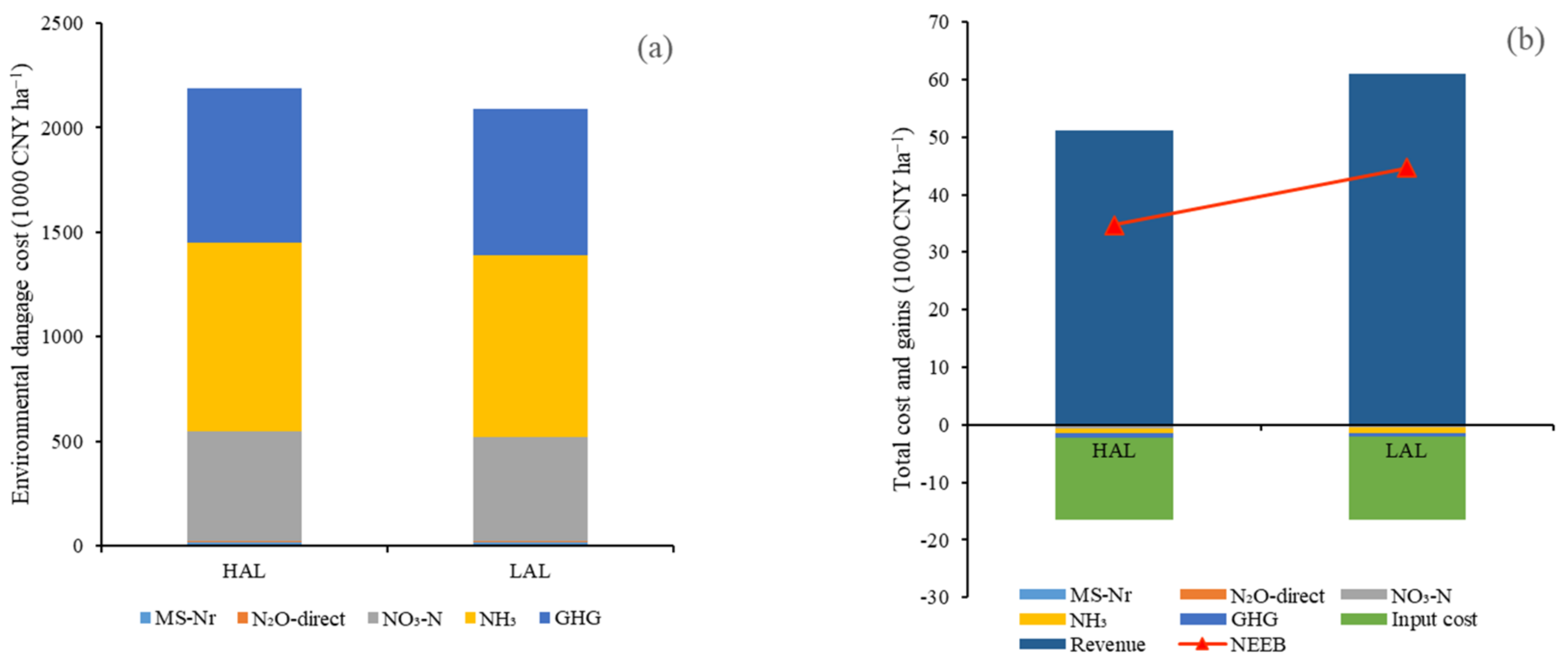
2.5. Environmental Damage Cost (EDC) and NEEB

The EDC (CNY ha⁻¹) represents the cost of C and Nr loss, including the estimated cost of soil acidification due to NH₃ release and eutrophication by nitrate (NO₃) leaching and runoff [21,22]. It was assessed using the following equation:

$$EDC=\underset{i=1}{\overset{m}{\Sigma }}{Nr}_i\times P_{{Nr}_i}+GHG emission\times P_{{CO}_2}$$

where Nr_i (kg N) represents the rate of i-th Nr loss; PNr_i (CNY kg⁻¹ N) represents the individual cost per unit of Nr; and GHG emission (t CO₂-eq ha⁻¹) and PCO₂ (CNY t (CO₂-eq)⁻¹) denote the total GHG emissions and cost per unit of CO₂, respectively (Table S4).

Net revenue (10³ CNY) was calculated as the yield revenue minus the cost of agricultural material on a per ha basis, and was calculated using the following equation:

$$Net revenue=Yield revenue-\underset{i=1}{\overset{m}{\Sigma }} {rate}_i\times P_i$$

Yield revenue was calculated by multiplying the pepper yield by the local market price of pepper. When determining the cost per ha of planted area of purchasing agricultural materials and hiring labor, i represents the material inputs, including fertilizers, pesticides, diesel, seeds, and labor; rate_i represents the application rate of the i-th input category; and P_i represents the purchase price of the i-th input category (Table S3).

The NEEB (CNY ha⁻¹) was calculated as follows:

$$NEEB=\mathrm{N}\mathrm{e}\mathrm{t} \mathrm{r}\mathrm{e}\mathrm{v}\mathrm{e}\mathrm{n}\mathrm{u}\mathrm{e}-\mathrm{E}\mathrm{D}\mathrm{C}$$

2.6. Environmental Cost of Products and Economic Benefit Assessment

The N and C footprints were used to express the GHG and Nr emissions per ton of pepper production, and were calculated as follows:

$$N footprint=Nr emission/Yield$$

$$C footprint=GHG emission/Yield$$

The NEEB for Nr and C emissions associated with pepper production was calculated using the following equations:

$${Nr}_{NEEB}=Nr emission/NEEB$$

$${GHG}_{NEEB}=GHG emission/NEEB$$

where Nr_NEEB and GHG_NEEB represent the CNY Yuan for Nr and GHG emissions, respectively. The Nr and GHG emissions were calculated on a per ha basis.

2.7. Yield Gap and Environmental Cost Analysis

The yield gap and environmental cost were analyzed via an LCA assessment and the quartering method [23], which categorized the 60 farmers into quartiles from high (quartile 1) to low (quartile 4) yield. The resource inputs and fresh yield of peppers in the four quartile groups are shown in

Table 2. The resource inputs and output for pepper cultivation in HAL and LAL. HAL represents the high-altitude level (500–800 m), and LAL represents the low-altitude level (900–1200 m).

Inventory	HAL			LAL
	Mean	Range	SD	Mean	Range	SD
Input
Total fertilizer (kg·ha−1)
N	297.3	169–484	73	289.3	163–539	76
P₂O₅	290.7	72–860	180	237.9	83–792	141
K₂O	154.7	0–511	105	236.9	0–477	94
Organic fertilizer (kg·ha−1)
Organic C	25.5	0–121	33	36.6	0–150	28
N	14.7	0–113	22	22.8	0–113	19
P₂O₅	19.0	0–113	28	29.0	0–113	22
K₂O
Inorganic fertilizers (kg·ha−1)	271.8	168–484	73	252.7	116–438	76
N	276.0	72–792	173	215.0	0–660	126
P₂O₅	135.7	0–477	100	208.0	0–432	85
K₂O	1.3	0–2.1	0.5	1.5	0–3	0.7
Pesticide (kg·ha−1)	52.1	0–120	13	53.4	26–109	13
Plastic cover (kg·ha−1)	2.9	0–105	16	8.6	0–45	12
Diesel (kg·ha−1)	0.75	-	-	0.75	-	-
Seed	4.5	-	-	4.5	-	-
Cultivation labor
Output
Fresh yield (t ha−1)	11.1	7.5–17.5	2.4	13.3	6.8–22.5	3.4
Net revenue (103 Yuan ha−1)	36.9	19.4–66.3	10.8	46.7	16.8–88.7	15.5

.

2.8. Statistical Analyses

Excel software was used to calculate the yield, resource inputs, Nr emission, GHG emissions, N footprint, C footprint, EDC and NEEB. The possibility of significant differences for the dependent variables mentioned above between the treatments (i.e., altitude level and farmer group categorized for the study area) was checked by means of an analysis of variance (ANOVA), using SigmaPlot (version 14.0; Systat Software, Inc., San Jose, CA, USA). Treatment means were compared using the least significant difference (LSD) at a 5% level of probability. In addition, linear regression models were performed to check whether fertilizer input and plant density have an influence on yield.

3. Results

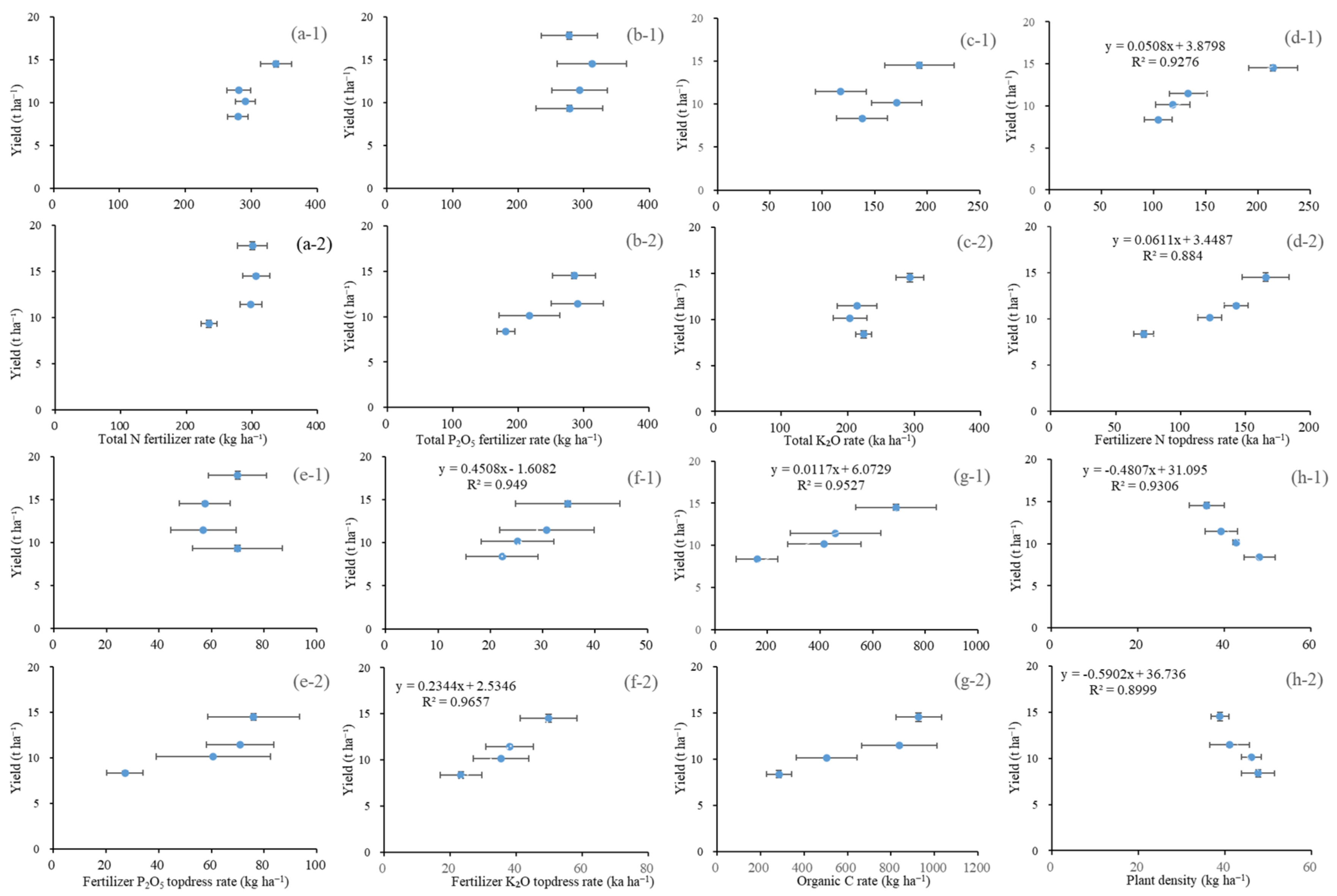
3.1. Yield and Resource Inputs

The yield and resource inputs associated with open-field pepper production at two altitudes are presented in Table 2. The average pepper yield at the HAL was 11.1 t ha⁻¹ (range: 7.5–17.5 t ha⁻¹), which was 16.2% lower than the average yield at the LAL (13.3 t ha⁻¹; range: 6.8–22.5 t ha⁻¹). The N and P fertilizer application rates at the HAL were 297.3 kg N ha⁻¹ and 290.7 kg P₂O₅ ha⁻¹, which were 4.22% and 19.3% higher than at the LAL (N: 285.3 kg N ha⁻¹, P: 243.6 kg P₂O₅ ha⁻¹), respectively. In contrast, the K fertilizer application rate at the HAL (154.7 kg K₂O ha⁻¹) was 33.8% lower than at the LAL (233.6 kg K₂O ha⁻¹). The application rates of pesticide and diesel were 13.1% and 66.6% lower at the HAL compared to the LAL, respectively. The plastic film application rate was similar between the altitudes. In summary, pepper production at high altitudes resulted in a lower yield, with higher N and P fertilizer applications.

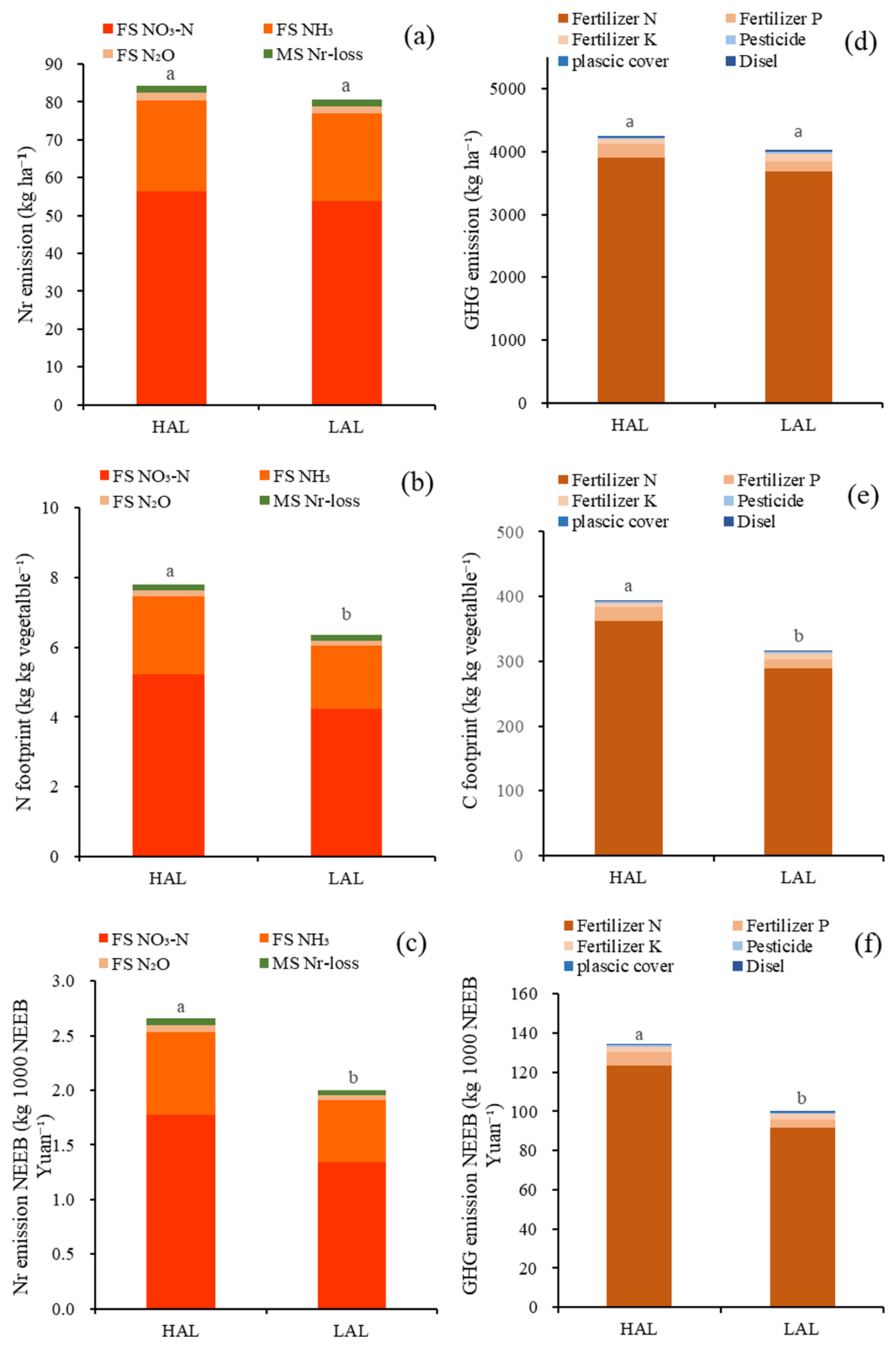
3.2. Nr Emissions, N Footprint, and NrNEEB

When expressed on a per ha of planted area basis, the average Nr emissions were comparable at the HAL (84.4 kg N ha⁻¹) and LAL (80.6 kg N ha⁻¹) (Figure 1). However, there were significant differences in the N footprint and Nr_NEEB between the two altitudes. The mean N footprint (7.8 kg N t⁻¹) at the HAL was 23.0% greater than at the LAL (6.4 kg N t⁻¹). The Nr_NEEB at the HAL (2.7 kg N Yuan⁻¹) was 32.6% greater than at the LAL (2.0 kg N Yuan⁻¹). At both high and low altitudes, the nitrate-nitrogen (NO₃-N) emissions in the FS were the largest contributor to Nr emissions, accounting for 67% of the total. The ammonia nitrogen (NH₃-N) released during the FS (28%) made the second largest contribution to the total Nr emissions, while N₂O emissions during the FS and Nr emissions during the MS accounted for less than 5% of the total.

3.3. GHG Emissions and C Footprint

When expressed on a per ha of planted area basis, the GHG emissions amount at the HAL was 4240 kg CO₂-eq ha⁻¹, which was 5.26% greater than at the LAL (4029 kg CO₂-eq ha⁻¹) (Figure 1). There were significant differences in GHG emissions between the two altitudes on a product (C footprint) and NEEB (GHG_NEEB) basis; the C footprint at the HAL (393.5 kg CO₂-eq t⁻¹) was 24.0% greater than at the LAL (317.3 kg CO₂-eq t⁻¹) and the GHG_NEEB at the HAL (134.1 kg CO₂-eq 10³ yuan⁻¹) was 33.8% greater than at the LAL (100.3 kg CO₂-eq 10³ yuan⁻¹) (Figure 1). The resource input that made the largest contribution to total GHG emissions was N fertilizer (91.3–92.1%); the other inputs only contributed to 7.9–8.7% of the total GHG emissions.

3.4. NEEB, Nr-_NEEB, and GHG-_NEEB

The EDC of pepper production is shown in Figure 2. The total EDC values at the HAL and LAL were 2.19 × 10³ and 2.09 × 10³ Yuan ha⁻¹, accounting for 7.0% and 5.6% of the total revenue, respectively. No significant difference in the EDC was observed between the two altitudes. Ammonia was the dominant contributor to the EDC, accounting for around 41% of the total; GHG emissions (34%) made the second most important contribution, followed by NO₃-N (24%). The other contributors (N₂O-direct and MS-Nr) accounted for less than 1% of the total. Due to the lower yield, the revenue at the HAL (51.2 × 10³ Yuan ha⁻¹) was 16.2% lower than at the LAL (61.1 × 10³ yuan ha⁻¹). On the other hand, agricultural material costs and the EDC were similar between the two altitudes. Thus, the NEEB at the HAL (34.7× 10³ NEEB Yuan ha⁻¹) was significantly lower (by 22.3%) than at the LAL (44.7 × 10³ NEEB Yuan ha⁻¹). The difference between the Nr_NEEB and GHG_NEEB was enhanced by the large difference in NEEB between the high and low altitudes. The Nr_NEEB and GHG_NEEB at the HAL were 32.6% and 33.8% lower than at the LAL, respectively.

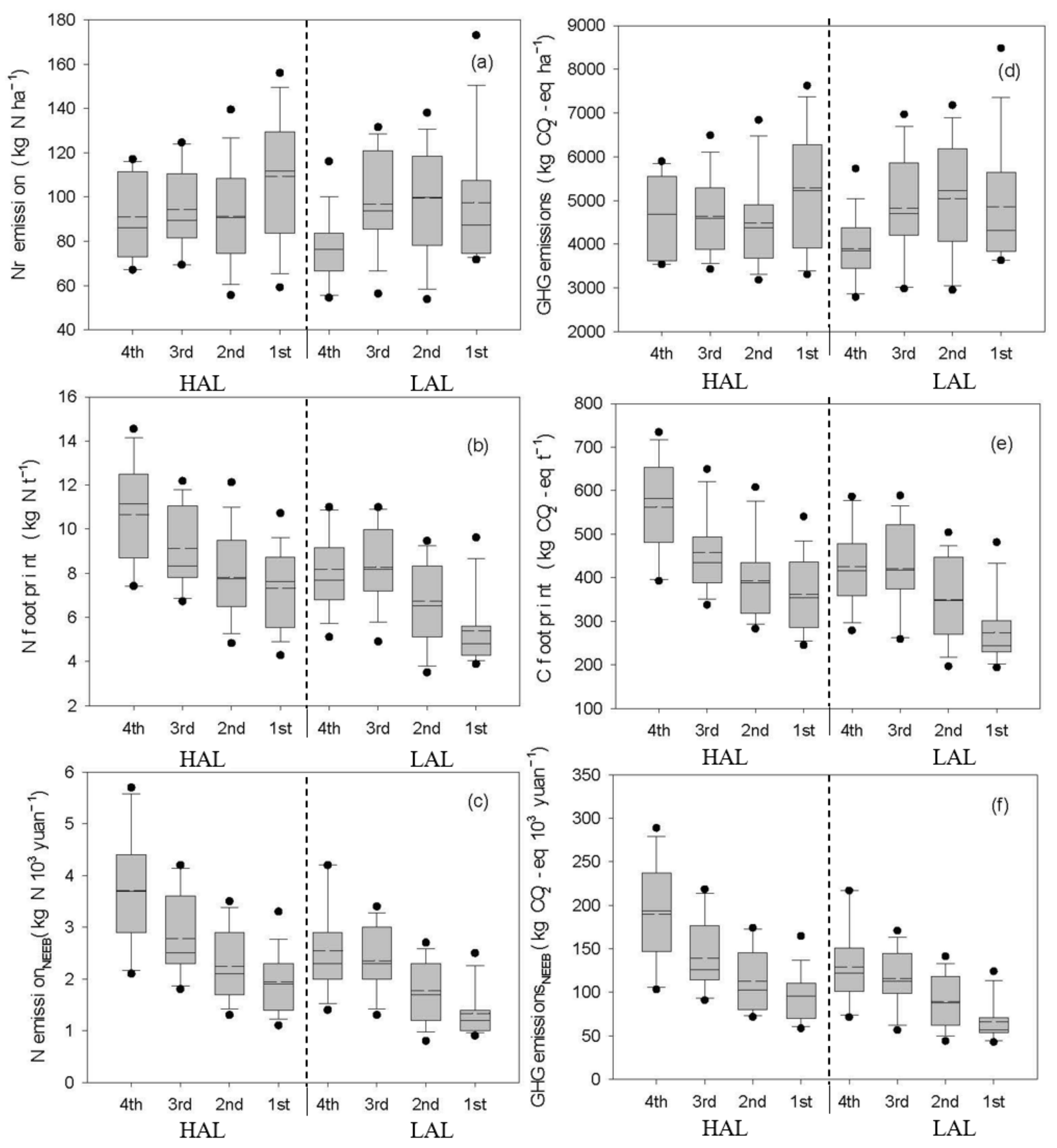
3.5. Yield Gap and Environmental Cost

There was a large yield gap among the four groups at both altitudes. Relative to quartile group 1, at the same altitude, the yields in groups 2–4 were 42.4%, 30.1%, and 21.1% lower at the HAL, and 47.8%, 35.8%, and 18.4% lower at the LAL, respectively (

Table 3. Resource input rate and output of open-field pepper production system among different farmers groups in HAL and LAL.

	HAL				LAL
	4th	3rd	2nd	1st	4th	3rd	2nd	1st
Total fertilizer
N (kg ha−1)	279.6 + 59.8	290.9 + 57.4	281.1 + 69.7	337.6 + 90.1	234.6 + 47.2	298.8 + 66	306.6 + 80.4	301.1 + 88.3
P2O5 (kg ha−1)	278.4 + 196.1	293.8 + 164.7	312.5 + 205.5	278 + 165.1	181.4 + 52.6	217.1 + 180	290.5 + 154.2	285.6 + 126.4
K2O (kg ha−1)	137.9 + 94.1	170.8 + 92	117.6 + 94.9	192.5 + 128.2	223.8 + 45.9	203.2 + 97.2	214 + 116.4	293.3 + 82.3
Inorganic fertilizer (kg ha−1)
N	267.3 + 57.6	261.6 + 57.8	260 + 74.7	298.4 + 94.8	208.4 + 48.8	268.6 + 76.8	277.1 + 84.8	256.8 + 75.6
P₂O₅	271.6 + 192.5	276.3 + 163.3	295.3 + 191.8	261 + 159.6	165 + 53.8	167.7 + 111.3	273.5 + 162.6	253.9 + 119.6
K₂O	129.5 + 85	147.4 + 88.4	98.7 + 98.4	167.2 + 120.1	202.6 + 46.4	185.7 + 86.5	192.8 + 112.2	250.8 + 73.1
Organic fertilizer (kg ha−1)
Organic C	161 + 309	309 + 337	318 + 513	629 + 510	296 + 220	593 + 597	839 + 669	1004 + 486
N	12.4 + 24.6	29.3 + 33.4	21.1 + 34	39.2 + 35.1	26.2 + 20.5	35.5 + 35.6	33.5 + 26.8	51 + 23.9
P₂O₅	6.9 + 14	17.6 + 23.1	17.3 + 33.1	17 + 13.2	16.4 + 9.5	26.2 + 26.9	17.1 + 16.2	31.7 + 16.5
K₂O	8.5 + 16.2	23.4 + 30.3	18.9 + 35.1	25.3 + 25.9	21.9 + 15.9	31 + 25.6	21.3 + 19.7	41.8 + 19.9
Pesticide (kg ha−1)	1.2 + 0.6	1.4 + 0.5	1.3 + 0.5	1.4 + 0.3	1.8 + 0.7	1.6 + 0.8	1.4 + 0.7	1.3 + 0.5
Plastic cover (kg ha−1)	48 + 13.8	51.5 + 2.6	55 + 14.4	54 + 15.8	56.8 + 14.8	51 + 8.8	52.9 + 17.5	53 + 8.1
Diesel (kg ha−1)	1.5 + 5.8	0 + 0	2 + 7.7	8 + 31	4.3 + 9.5	7.4 + 11.8	12.4 + 14.5	10.5 + 12.9
Fresh yield (kg ha−1)	8.37 + 0.68	10.15 + 0.5	11.46 + 0.45	14.53 + 1.32	9.33 + 1.43	11.44 + 0.34	14.53 + 0.73	17.8 + 1.74
Net revenue (1000 ha−1)	9.76 + 2.85	14.22 + 2.07	18.23 + 2.07	25.94 + 3.95	12.34 + 4.12	18.2 + 1.79	26.32 + 2.59	35.15 + 5.17

The value represented the mean ± standard deviation (SD).

). The corresponding total N fertilizer application rate in group 1 (337.6 kg ha⁻¹) was significantly higher than in the other three groups (279.6–290.9 kg ha⁻¹) at the HAL (Table 3). However, the total N fertilizer (301.1 kg N ha⁻¹) application rate in group 1 at the LAL was comparable to that of groups 2 (306.6 kg N ha⁻¹) and 3 (298.8 kg N ha⁻¹) (Table 3). At the LAL, group 1 achieved a higher yield without any increase in the N fertilizer input. Group 1 had the greatest NEEB among the four groups at the HAL; it was 36.6, 30.2, and 22.6 × 10³ Yuan higher than for groups 2–4, respectively (i.e., 206.0%, 94.3%, and 45.4% higher, respectively). Similarly, the difference in NEEB between group 1 and the other three groups was in the range of 14.8–37.5 10³ Yuan at the LAL, i.e., the NEEB for group 1 was 29.5–137.6% greater than in the other three groups (Table 3).

When expressed on an area basis, at the HAL, the Nr and GHG emissions for group 1 were 15.2–15.9% and 12.5–13.9% higher than in groups 2 and 3, respectively. However, the Nr (84.5 kg N ha⁻¹) and GHG (4201 kg CO₂-eq t⁻¹) emissions in group 1 at the LAL were comparable to those of groups 2 (87.2 kg N ha⁻¹, 4403 kg CO₂-eq t⁻¹) and 3 (84.9 kg N ha⁻¹, 4188 kg CO₂-eq t⁻¹). When expressed on a product basis, the N “footprint gaps” at the HAL were 3.1, 1.6, and 0.5 kg N kg⁻¹ for groups 4, 3 and 2, respectively, i.e., group 1 contributed 48.5%, 24.9% and 7.9% less to the N footprint than groups 4, 3 and 2 at the HAL, respectively. The corresponding C footprint gaps were 170.9, 84.0, and 32.5 CO₂-eq kg⁻¹ relative to group 1 at the HAL, i.e., group 1 contributed 34.7%, 20.7%, and 9.2% less to the C footprint than groups 4, 3 and 2 at the HAL. Similarly, groups 4, 3 and 2 at the LAL had N footprint gaps of 2.4, 2.6, and 1.2 kg N kg⁻¹, and C footprint gaps of 124.9, 128.4, and 67.0 kg CO₂-eq kg⁻¹, compared to group 1 at the LAL, respectively. Compared to group 1, the N footprint of groups 2–4 at the LAL was 26.2%, 55.2%, and 50.5% lower, respectively, and the C footprint was 22.0%, 35.1%, and 34.5%, lower. Compared to the average values reported by the farmers surveyed at the same altitude level, the N and C footprints in group 1 were lower by 16.9% and 18.3% at the HAL, and by 24.8% and 25.2% at the LAL, respectively. The Nr_NEEB and GHG_NEEB gap between group 1 and the other groups was enhanced by the large NEEB gap. In group 1, the Nr_NEEB was 15.3–92.1% lower, and the GHG_NEEB was 17.6–98.1% lower than in the other three groups at the same altitude level.

4. Discussion

4.1. Environmental Cost of Pepper Production at Different Altitudes

Both economic and physiological factors drive the high environmental cost of vegetable production [24]. Our results demonstrated that high-altitude vegetable production resulted in higher Nr and GHG emissions than low-altitude production. On an area basis, due to the higher resource input, Nr (84.4 kg N ha⁻¹) and GHG (4240 kg CO₂-eq ha⁻¹) emissions were higher than reported in previous studies of other low-altitude vegetable production systems (Nr emission: 43 kg N ha⁻¹, GHG emission: 4638–4854 kg CO₂-eq ha⁻¹; [25]). However, the emissions were lower than reported for greenhouse vegetable production (GHG emission: 7061–19,820 kg CO₂-eq ha⁻¹; [3,26]), due to the additional structural materials (metal, plastic, irrigation facilities, etc.) and resources (electricity, water) required in greenhouses compared to open-field production systems. Greenhouse system emissions are much higher than in grain production systems (GHG emission: 2210–3629 kg CO₂-eq ha⁻¹; [27,28]) due to the higher resource inputs. On a yield basis, the N and C footprints at the HAL were also higher than for other vegetable systems, mainly due to the lower yield. For example, the average N footprint (7.6 kg N t⁻¹) at the HAL was 348% higher than at the LAL (2.1 kg N t⁻¹) due to the higher yield at the former level (11.1 t ha⁻¹). This was still far below the “ox horn” pepper yield reported in the eastern plains area of China (41 t ha⁻¹) [29].

There was a large difference in the N and C footprints between the high and low altitudes in this study. Compared to the LAL, the N and C footprints at the HAL were 23.0% and 24.0% higher, respectively. There were several reasons for this. First, fertilizer was the main source of Nr and GHG emissions [30]. Compared to the LAL, the total N and P fertilizer input at the HAL was 4.2% and 19.3% higher, respectively, which could be attributed to the higher runoff loss associated with the steeper slope (13°, Table 1) in the arable area at the HAL [31,32]. Second, the type of fertilizer (organic or inorganic fertilizer) had an important effect on Nr and GHG emissions during vegetable production [33]. Compared to N from organic fertilizers, inorganic N fertilizer contributed 18.7–22.2% of the runoff per unit N input [34]. This resulted in the Nr and GHG emissions on an area basis being 4.6% and 5.3% greater at the HAL than the LAL, respectively. Third, yield also exerted an important influence on the Nr and C footprints [35,36], with the yield at the HAL being 16.2% lower than at the LAL. This large variation in yield was the main driver of the higher N and C footprints at the HAL. The pepper yield was higher at the LAL than the HAL. There are several explanations for this. First, the climate differs by altitude [37]. The optimal temperature range for pepper cultivation is 25–31 °C [38,39]. The temperature during the growth stage at the LAL (22.7 °C) in this study was more suitable than at the HAL (18.6 °C). Soil properties also play an important role in pepper production [28,40]. The optimum soil pH range for pepper production is 6.2–8.5 [40,41], so the pH (5.3 ± 0.96) at the HAL may have had a more adverse impact on pepper yield than the higher pH at the LAL (6.1 ± 1.3). Third, the production conditions affected the yields at the two altitudes. The HAL had a poor road system and uneven vegetable fields, both of which are very important with respect to the accessibility of yield-improving technology and agricultural machinery. For example, the poor road system at the HAL limited the application of agricultural machinery and organic fertilizer. Compared to the LAL, the diesel consumed by agricultural machinery and organic C applied at the HAL were 66.6% and 32.4% lower, respectively (Table 2).

The Nr_NEEB and GHG_NEEB at the LAL were 32.6% and 33.8% lower than at the HAL, mainly due to the lower yield and net revenue at the HAL. At the HAL, farmers applied excessive resource inputs to overcome the N and P runoff losses and obtain high pepper yields. Their lack of nutrient management expertise resulted in large resource input costs. The higher cost combined with lower total revenue due to the lower yield resulted in a lower net revenue at the HAL.

Overall, pepper production at high altitudes resulted in higher Nr and GHG emissions, larger N and C footprints and lower yields, net profit, and NEEB. This clearly showed that the expansion of pepper cultivation to higher altitudes was associated with greater environmental costs and relatively smaller economic benefits.

4.2. Potential for Mitigating Environmental Costs

The N and C footprints of group 1 were 7.9%, 24.9%, 48.5%, and 16.9%, and 9.2%, 23.7%, 48.3% and 18.3%, lower than in groups 2–4 and the average at the HAL, respectively (Figure 3). Closure of yield gaps offers great potential for mitigating the environmental cost of agricultural systems [35]. Although the Nr and GHG emissions at the HAL were the largest in group 1 in this study, mainly due to the higher fertilizer input than in the other groups, the increase in the rate of N fertilizer application was 17% lower than the rate of yield increase in group 1. This resulted in a smaller N and C footprint at the HAL in group 1 compared to the other groups and the average for all farmers. Many studies [12,15,42] have indicated that the yield gap can be closed by improving crop and nutrient management by adopting best-practice farming methods. However, the factors responsible for the yield gap differ among regions and crops due to large variations in climate, soil conditions, and management practices. In this study, the higher yield in group 1 at the HAL and LAL could be explained by several factors. The top-dress fertilizer rate, especially the N and K fertilizer rate, was the major factor influencing vegetable yield. Our results revealed positive relationships between the N fertilizer top-dressing rate and yield. An increase in the N and K fertilizer application rates promoted rapid crop growth and fruit formation at the later growth stage [43]. There were no significant relationships between the total N, P, and K fertilizer application rates and yield (Figure 4). Second, regarding organic management, organic fertilizer application can also improve soil quality, reduce soil Nr loss, and promote crop growth [44,45]. Due to long-term and excessive inorganic fertilizer inputs, several soil problems (e.g., acidification, soil-borne disease, and decreased quantity and stability of structural aggregates) are very common in the survey area. Our results revealed a positive relationship between the organic C input rate and yield. Additional organic C inputs improve soil structure, stimulate soil microbial activity, and improve the yield of vegetable crops. Third, regarding management, an appropriate planting density will be able to fully exploit the light conditions and soil nutrients. Our results indicated that an excessive planting density would have a negative influence on pepper yield (Figure 4). This might result in undue competition between plants for limited light and heat, thereby reducing carbohydrate production [46]. In addition, there was room for further optimization of group 1. The N and P fertilizer input was much higher than the vegetable demand and recommended fertilization rate (147–200 kg N ha⁻¹, 75–90 kg P₂O₅ ha⁻¹) [47], which could be optimized with in-season root-zone nutrient management to match the nutrient supply [12]. Furthermore, the traditional N fertilizer (e.g., urea, ammonium carbonate) applied in the survey area could be substituted for an N fertilizer with a nitrification inhibitor [48,49].

In the future, it will be important to consider the environmental cost of resource inputs, and their mitigation potential in the context of vegetable production at high altitudes. For the first time, this study systemically compared the environmental cost of resource inputs for pepper production between high and low altitudes. Our results indicated that pepper production at high altitudes was more resource-intensive and led to larger N and C footprints than production at low altitudes. The results provide a reference for studies of the environmental cost of crop production in other high-altitude regions of the world. We quantified the environmental cost of pepper production at high altitudes in southwest China and identified potential mitigation measures. The results indicated that the pepper yield could be improved, while the environmental cost was greatly diminished by optimizing crop and nutrient management. These results have important implications for sustainable vegetable production in high-altitude regions. However, the uncertainty of this research is that we surveyed the Shizhu of southwest China, which is a local characteristic; for future research, we recommend wider coverage and longer-term experimentation for a higher level of generalization.

5. Conclusions

The results of this study indicated that open-field pepper production at high altitudes had higher resource inputs and lower yields than production at low altitudes, resulting in 4.6% and 5.3% higher Nr and C emissions on an area basis, and 23.0% and 24.0% higher N and C footprints on a product basis. There is considerable potential for yield increases and mitigation of the environmental cost at high altitudes. Compared to the average for all farms, the high-yield group contributed 12.4% and 18.3% less to the overall C and N footprints, mainly due to their higher yields. Reducing plant density and increasing the topdressing fertilizer rate and organic C inputs could improve the pepper yield and decrease the N and C footprints.

References

1. Xiang, Q.; Yu, H.; Xu, X.; Huang, H. Temporal and Spatial Differentiation of Cultivated Land and Its Response to Climatic Factors in Complex Geomorphic Areas—A Case Study of Sichuan Province of China. Land 2022, 11, 271. [Google Scholar] [CrossRef]
2. Yao, Z.; Zhang, L.; Tang, S.; Li, X.; Hao, T. The basic characteristics and spatial patterns of global cultivated land change since the 1980s. J. Geogr. Sci. 2017, 27, 771–785. [Google Scholar] [CrossRef] [Green Version]
3. Liang, T.; Liao, D.X.; Wang, S.; Yang, B.; Zhao, J.K.; Zhu, C.F.; Zhang, T.; Shi, X.J.; Chen, X.P.; Wang, X. The nitrogen and carbon footprints of vegetable production in the subtropical high elevation mountain region. Ecol. Indic. 2020, 122, 107298. [Google Scholar] [CrossRef]
4. Yu, Z.; Liu, J.; Kattel, G. Historical nitrogen fertilizer use in China from 1952 to 2018. Earth Syst. Sci. Data 2022, 14, 5179–5194. [Google Scholar] [CrossRef]
5. Miao, T.T.; Wang, B.; Cai, A.; Ren, T.J.; Wan, Y.F.; Meng, Y.; Li, Y. Large differences in ammonia emission factors between greenhouse and open-field systems under different practices across Chinese vegetable cultivation. Sci. Total Environ. 2022, 852, 158339. [Google Scholar] [CrossRef]
6. Fan, C.H.; Li, B.; Xiong, Z.Q. Nitrification inhibitors mitigated reactive gaseous nitrogen intensity in intensive vegetable soils from China. Sci. Total Environ. 2017, 612, 480–489. [Google Scholar] [CrossRef]
7. Martínez-Blanco, J.; Muñoz, P.; Antón, A.; Rieradevall, J. Assessment of tomato Mediterranean production in open-field and standard multi-tunnel greenhouse, with compost or mineral fertilizers, from an agricultural and environmental standpoint. J. Clean. Prod. 2011, 19, 985–997. [Google Scholar] [CrossRef]
8. Payen, S.; Basset-Mens, C.; Perret, S. LCA of local and imported tomato: An energy and water trade-off. J. Clean. Prod. 2014, 87, 139–148. [Google Scholar] [CrossRef]
9. Xia, L.L.; Xia, Y.Q.; Li, B.; Wang, J.Y.; Wang, S.W.; Zhou, W.; Yan, X.Y. Integrating agronomic practices to reduce greenhouse gas emissions while increasing the economic return in a rice-based cropping system. Agric. Ecosyst. Environ. 2016, 231, 24–33. [Google Scholar] [CrossRef] [Green Version]
10. Stefano, M.; Alicia, L.; Reyes, T. Greenhouse gas emissions from global production and use of nitrogen synthetic fertilisers in agriculture. Sci. Rep. 2022, 12, 14490. [Google Scholar] [CrossRef]
11. Xia, L.L.; Cao, L.; Yang, Y.; Ti, C.; Liu, Y.; Smith, P.; Groenigen, K.; Lehmann, J.; Lal, R.; Butterbach-Bahl, K.; et al. Integrated biochar solutions can achieve carbon-neutral staple crop production. Nat. Food 2023. [Google Scholar] [CrossRef]
12. Kalimuthu, S. Closing rice yield gaps in Africa requires integration of good agricultural practices. Field Crops Res. 2022, 285, 108591. [Google Scholar] [CrossRef]
13. Bojaca, C.R.; Wyckhuys, K.A.G.; Schrevens, E. Life cycle assessment of Colombian greenhouse tomato production based on farmer-level survey data. J. Clean. Prod. 2014, 69, 26–33. [Google Scholar] [CrossRef]
14. Baral, R.; Kafle, B.; Panday, D.; Shrestha, J.; Min, D. Adoption of Good Agricultural Practice to Increase Yield and Profit of Ginger Farming in Nepal. J. Hortic. Res. 2021, 29, 55–66. [Google Scholar] [CrossRef]
15. Wang, X.Z.; Zou, C.Q.; Zhang, Y.; Shi, X.; Liu, Y.M.; Liu, J.Z.; Fan, S.S.; Du, Y.F.; Zhao, Q.Y.; Tan, Y.G.; et al. Environmental impacts of pepper (Capsicum annuum L.) production affected by nutrient management: A case study in southwest China. J. Clean. Prod. 2018, 171, 934–943. [Google Scholar] [CrossRef]
16. Awio, T.; Senthilkumar, K.; Dimkpa, C.O.; Otim-Nape, G.W.; Struik, P.C.; Stomph, T.J. Yields and Yield Gaps in Lowland Rice Systems and Options to Improve Smallholder Production. Agronomy 2022, 12, 552. [Google Scholar] [CrossRef]
17. Oliver, Y.; Robertson, M. Quantifying the spatial pattern of the yield gap within a farm in a low rainfall Mediterranean climate. Field Crops Res. 2013, 150, 29–41. [Google Scholar] [CrossRef]
18. Wang, X.Z.; Liu, B.; Wu, G.; Sun, Y.X.; Guo, X.S.; Jin, Z.H.; Xu, W.N.; Zhao, Y.Z.; Zhang, F.S.; Zou, C.Q.; et al. Environmental costs and mitigation potential in plastic-greenhouse pepper production system in China: A life cycle assessment. Agric. Syst. 2018, 167, 186–194. [Google Scholar] [CrossRef]
19. Xie, L.H.; Li, L.; Xie, J.H.; Wang, J.B.; Anwar, S.; Du, C.L.; Zhou, Y.J. Substituting Inorganic Fertilizers with Organic Amendment Reduced Nitrous Oxide Emissions by Affecting Nitrifiers’Microbial Community. Land 2022, 11, 1702. [Google Scholar] [CrossRef]
20. Antille, D.L.; Macdonald, B.C.T.; Uelese, A.; Webb, M.J.; Kelly, J.; Tauati, S.; Stockmann, U.; Palmer, J.; Barringer, J.R.F. Toward Soil Nutrient Security for Improved Agronomic Performance and Increased Resilience of Taro Production Systems in Samoa. Soil Syst. 2023, 7, 21. [Google Scholar] [CrossRef]
21. Cai, S.Y.; Pittelkow, C.; Zhao, X.; Wang, S.Q. Winter legume-rice rotations can reduce nitrogen pollution and carbon footprint while maintaining net ecosystem economic benefits. J. Clean. Prod. 2018, 195, 289–300. [Google Scholar] [CrossRef]
22. Lam, S.; Suter, H.; Bai, M.; Walker, C.; Mosier, A.; Grinsven, H.; Chen, D. Decreasing ammonia loss from an Australian pasture with the use of enhanced efficiency fertilizers. Agric. Ecosyst. Environ. 2019, 283, 106553. [Google Scholar] [CrossRef]
23. Mohammadi-Kashka, F.; Pirdashti, H.; Tahmasebi-Sarvestani, Z.; Motevali, A.; Nadi, M.; Aghaeipour, N. Integrating life cycle assessment (LCA) with boundary line analysis (BLA) to reduce agro-environmental risk of crop production: A case study of soybean production in Northern Iran. Clean Technol. Environ. Policy 2023. [Google Scholar] [CrossRef]
24. Félix, O.; Tapsoba, P.K. Diversity of market gardening farms in western Burkina Faso. Nexus between production environment, farm size, financial performance and environmental issues. Heliyon 2022, 8, 12408. [Google Scholar] [CrossRef]
25. Zarei, M.J.; Kazemi, N.; Marzban, A. Life cycle environmental impacts of cucumber and tomato production in open-field and greenhouse. J. Saudi Soc. Agric. Sci. 2019, 18, 249–255. [Google Scholar] [CrossRef]
26. He, X.Q.; Qiao, Y.H.; Liu, Y.X.; Dendler, L.; Yin, C.; Martin, F. Environmental impact assessment of organic and conventional tomato production in urban greenhouses of Beijing city, China. J. Clean. Prod. 2016, 134, 251–258. [Google Scholar] [CrossRef]
27. Bernesson, S.; Daniel, N.; Per-Anders, H. A limited LCA comparing large-and small-scale production of ethanol for heavy engines under Swedish conditions. Biomass Bioenergy 2006, 30, 46–57. [Google Scholar] [CrossRef]
28. Zhao, R.R.; He, P.; Xie, J.G.; Johnston, A.; Xu, X.P.; Qiu, S.J.; Zhao, S.C. Ecological intensification management of maize in northeast China: Agronomic and environmental response. Agric. Ecosys. Environ. 2016, 224, 123–130. [Google Scholar] [CrossRef]
29. Wang, X.Z.; Liu, B.; Gang, W.; Sun, Y.X.; Guo, X.S.; Jin, G.Q.; Jin, Z.H.; Zou, C.Q.; Dave, C.; Chen, X.P. Cutting carbon footprints of vegetable production with integrated soil-crop system management: A case study of greenhouse pepper production. J. Clean. Prod. 2020, 254, 120–158. [Google Scholar] [CrossRef]
30. Liang, L.; Ridoutt, B.G.; Lal, R.; Wang, D.P.; Wu, W.L.; Peng, P.; Hang, S.; Wang, L.Y.; Zhao, G.S. Nitrogen footprint and nitrogen use efficiency of greenhouse tomato production in North China. J. Clean. Prod. 2018, 208, 285–296. [Google Scholar] [CrossRef]
31. Preltl, G.; Romeo, M.; Bacchi, M.; Monti, M. Soil loss measure from Mediterranean arable cropping systems: Effects of rotation and linage system on C-factor. Soil. Till. Res. 2017, 170, 85–93. [Google Scholar] [CrossRef]
32. Zhong, X.; Zhang, L.; Yue, X.R.; Xia, Y.S. Soil N and P Loss in slope Farmland of Dianchi Watershed. J. Soil Water Conserv. 2018, 32, 42–46. (In Chinese) [Google Scholar] [CrossRef]
33. Holka, M.; Kowalska, J.; Jakubowska, M. Reducing Carbon Footprint of Agriculture—Can Organic Farming Help to Mitigate Climate Change? Agriculture 2022, 12, 1383. [Google Scholar] [CrossRef]
34. Shan, L.; He, Y.F.; Chen, J.; Huang, Q. Nitrogen surface runoff losses from a Chinese cabbage field under different nitrogen treatments in the Taihu Lake Basin, China. Agric. Water. Manag. 2015, 159, 255–263. [Google Scholar] [CrossRef]
35. Cui, Z.L.; Wang, G.; Yue, S.C.; Wu, L.; Zhang, W.F.; Zhang, F.; Chen, X. Closing the N-Use Efficiency Gap to Achieve Food and Environmental Security. Environ. Sci. Technol. 2014, 48, 5780–5787. [Google Scholar] [CrossRef] [PubMed]
36. Davies, W.; Ward, S.; Wilson, A. Can crop science really help us to produce more better-quality food while reducing the world-wide environmental footprint of agriculture. Front. Agric. Sci. Eng. 2020, 7, 28–44. [Google Scholar] [CrossRef] [Green Version]
37. Tanyi, C.; Ngosong, C.; Ntonifor, N. Effects of climate variability on insect pests of cabbage: Adapting alternative planting dates and cropping pattern as control measures. Chem. Biol. Technol. Agric. 2018, 5, 25. [Google Scholar] [CrossRef] [Green Version]
38. O’Sullivan, J.; Bouw, W.J. Pepper seed treatment for low-temperature germination. Can. J. Plant Sci. 1984, 64, 387–393. [Google Scholar] [CrossRef]
39. Coons, J.; Kuehl, R.; Oebker, N.; Simons, N. Seed germination of seven pepper cultivars at constant or alternating high temperatures. J. Hortic. Sci. 1989, 64, 705–710. [Google Scholar] [CrossRef]
40. Russo, V.M. Peppers, Botany, Production and Uses; USDA/ARS Wes Watkins Agricultural Research Laboratory: Lane, OK, USA; Wallingford, CT, USA, 2012; Available online: http://library.wur.nl/WebQuery/clc/1981465 (accessed on 11 February 2020).
41. Chen, X.; Wu, G. Protected-Land Pepper Cultivation; Golden Shield Press: Beijing, China, 2010. (In Chinese) [Google Scholar]
42. Wang, N.; Jassogne, L.; Asten, P.; Mukasa, D.; Wanyama, I.; Kagezi, G.; Giller, K. Evaluating coffee yield gaps and important biotic, abiotic, and management factors limiting coffee production in Uganda. Eur. J. Agron. 2015, 63, 1–11. [Google Scholar] [CrossRef]
43. Dhillon, J.; Eickhoff, E.; Aula, L.; Omara, P.; Weymeyer, G.; Nambi, E.; Oyebiyi, F.; Carpenter, T.; Raun, W. Nitrogen management impact on winter wheat grain yield and estimated plant nitrogen loss. Agron. J. 2020, 112, 564–577. [Google Scholar] [CrossRef] [Green Version]
44. Tian, S.Y.; Zhu, B.J.; Yin, R.; Wang, M.W.; Jiang, Y.J.; Zhang, C.Z.; Li, D.M.; Chen, X.Y.; Kardol, P.; Liu, M.Q. Organic fertilization promotes crop productivity through changes in soil aggregation. Soil Biol. Biochem. 2021, 165, 108533. [Google Scholar] [CrossRef]
45. Zhang, M.; Li, B.; Xiong, Z.Q. Effects of organic fertilizer on net global warming potential under an intensively managed vegetable field in southeastern China: A three years field study. Atmos. Environ. 2016, 145, 92–103. [Google Scholar] [CrossRef]
46. Casal, J.; Deregibus, V.; Sanchez, R. Variations in tiller dynamics and morphology in Lolium multiflorum Lam. Vegetative and reproductive plants as affected by differences in red/far-red irradiation. Ann. Bot. 1985, 56, 553–559. [Google Scholar] [CrossRef]
47. Chongqing Agricultural Technology Station. The Main Vegetable Fertilizer Recommended Formula. 2020. Available online: http://www.cqates.com/details.aspx?topicId=752786&ci=1673&psi=104 (accessed on 12 April 2020).
48. Fan, C.H.; Leng, Y.F.; Zhang, Q.; Zhao, X.W.; Gao, W.L.; Duan, P.P.; Li, Z.L.; Luo, G.W.; Zhang, W.; Chen, M.; et al. Synergistically mitigating nitric oxide emission by co-applications of biochar and nitrification inhibitor in a tropical agricultural soil. Environ. Res. 2022, 214, 113989. [Google Scholar] [CrossRef] [PubMed]
49. Hargreaves, P.R.; Baker, K.L.; Graceson, A.; Bonnett, S.A.F.; Ball, B.C.; Cloy, J.M. Use of a nitrification inhibitor reduces nitrous oxide (N2O) emissions from compacted grassland with different soil textures and climatic conditions. Agric. Ecosyst. Environ. 2021, 310, 107307. [Google Scholar] [CrossRef]
50. Zhang, W.-F.; Dou, Z.-X.; He, P.; Ju, X.-T.; Powlson, D.; Chadwick, D.; Norse, D.; Lu, Y.-L.; Zhang, Y.; Wu, L.; et al. New technologies reduce greenhouse gas emissions from nitrogenous fertilizer in China. Proc. Natl. Acad. Sci. USA 2013, 110, 8375–8380. [Google Scholar] [CrossRef] [PubMed] [Green Version]
51. Yue, S.C. Optimum Nitrogen Management for High-yielding Wheat and Maize Cropping System; China Agricultural University Press: Beijing, China, 2013; p. 80. [Google Scholar]
52. Pahlavan, R.; Omid, M.; Akram, A. Energy input–output analysis and application of artificial neural networks for predicting greenhouse basil production. Energy 2012, 37, 171–176. [Google Scholar] [CrossRef]
53. Clark, S.; Khoshnevisan, B.; Sefeedpari, P. Energy efficiency and greenhouse gas emissions during transition to organic and reduced-input practices: Student farm case study. Ecol. Eng. 2016, 88, 186–194. [Google Scholar] [CrossRef]
54. Cui, Z.; Yue, S.; Wang, G.; Zhang, F.; Chen, X. In-Season Root-Zone N Management for Mitigating Greenhouse Gas Emission and Reactive N Losses in Intensive Wheat Production. Environ. Sci. Technol. 2013, 47, 6015–6022. [Google Scholar] [CrossRef] [PubMed]
55. Pishgar-Komleh, S.H.; Omid, M.; Heidari, M.D. On the study of energy use and GHG (greenhouse gas) emissions in greenhouse cucumber production in Yazd province. Energy 2013, 59, 63–71. [Google Scholar] [CrossRef]
56. Wang, X.; Zou, C.; Gao, X.; Guan, X.; Zhang, W.; Zhang, Y.; Shi, X.; Chen, X. Nitrous oxide emissions in Chinese vegetable systems: A meta-analysis. Environ. Pollut. 2018, 239, 375–383. [Google Scholar] [CrossRef] [PubMed]
57. Ti, C.; Luo, Y.; Yan, X. Characteristics of nitrogen balance in open-air and greenhouse vegetable cropping systems of China. Environ. Sci. Pollut. Res. 2015, 22, 18508–18518. [Google Scholar] [CrossRef] [PubMed]
58. Fan, C.; Chen, H.; Li, B.; Xiong, Z. Biochar reduces yield-scaled emissions of reactive nitrogen gases from vegetable soils across China. Biogeosciences 2017, 14, 2851–2863. [Google Scholar] [CrossRef] [Green Version]
59. Lu, K. Optimized Management of Nitrogen Fertilizer and Strategies for Reducing Nitrogen Leaching Loss in Greenhouse Vegetable Field in Taihu Region. Ph.D. Thesis, Nanjing Agricultural University, Nanjing, China, 2011. [Google Scholar]
60. Min, J.; Zhang, H.L.; Shi, W.M. Optimizing nitrogen input to reduce nitrate leaching loss in greenhouse vegetable production. Agric. Water Manag. 2012, 111, 53–59. [Google Scholar] [CrossRef]
61. Xia, L.; Ti, C.; Li, B.; Xia, Y.; Yan, X. Greenhouse gas emissions and reactive nitrogen releases during the life-cycles of staple food production in China and their mitigation potential. Sci. Total Environ. 2016, 556, 116–125. [Google Scholar] [CrossRef]
Figure 1. Reactive N loss (ac) and greenhouse gas emission (df) on per ha, tonne of vegetable and 1000 NEEB Yuan basic of pepper production in HAL and LAL. HAL represents the high-altitude level (500–800 m), LAL represents the low-altitude level (900–1200 m). The lowercase letters represent significant differences according to least significant test (p < 0.05).
Land 12 00662 g001
Figure 2. Environmental damage costs (a) and total net ecosystem economic benefits (b) in HAL and LAL for open-field vegetable production. HAL represents the high-altitude level (500–800 m), and LAL represents the low-altitude level (900–1200 m).
Land 12 00662 g002
Figure 3. The Nr Emissions (a), N footprint (b), N emissionNEEB (c), GHG emission (d), C footprint (e) and GHGemissionNEEB (f) in different groups of open-field pepper production. The yield data from surveyed farmers were ordered from low to high and divided into four quartiles: 1st quartile (best 25%), 2nd quartile (50–75%), 3rd quartile (25–50%), and 4th quartile (lowest 25%). HAL represents the high-altitude level (500–600 m), and LAL represents the low-altitude level (900–1200 m).
Land 12 00662 g003
Figure 4. Relationships between yield and total N fertilizer rate, total P₂O₅ fertilizer rate, total K₂O fertilizer rate, N fertilizer top-dress, P₂O₅ fertilizer top-dress rate, K₂O fertilizer top-dress rate, Organic C, plant density in HAL (a-1h-1) and LAL (a-2h-2) for open-field vegetable production in southwest China.
Land 12 00662 g004